An Inexact Restoration Direct Multisearch Filter Approach to Multiobjective Constrained Derivative-free Optimization

Abstract

Direct Multisearch (DMS) is a well-established class of methods for multiobjective derivative-free optimization, where constraints are addressed by an extreme barrier approach, only evaluating feasible points. In this work, we propose a filter approach, combined with an inexact feasibility restoration step, to address constraints in the DMS framework. The filter approach treats feasibility as an additional component of the objective function, avoiding the computation of penalty parameters or Lagrange multipliers. The inexact restoration step attempts to generate new feasible points, contributing to prioritize feasibility, a requirement for the good performance of any filter approach. Theoretical results are provided, analyzing the different types of sequences of points generated by the new algorithm, and numerical experiments on a set of nonlinearly constrained biobjective problems are reported, stating the good algorithmic performance of the proposed approach.
Keywords: Derivative-free Optimization; Black-box optimization; Multiobjective Optimization; Constrained Optimization; Direct Multisearch; Filter methods; Inexact Restoration.
AMS Classification: 90C29, 90C30, 90C56, 65K05, 49J52.

1 Introduction

Multiobjective optimization is a challenging scientific domain, not only from a theoretical point of view but also due to its extensive range of applications [15, 31, 41, 46]. The presence of several conflicting objectives, that need to be simultaneously optimized, changes the classical concept of problem solution, which is no longer a single point. The goal is to identify a set of nondominated points, meaning that it is impossible to simultaneously improve all components of the objective function for each one of these points.

This set of nondominated points is denominated as Pareto front and constitutes the solution of the multiobjective optimization problem. It can be supported by a convex, a nonconvex, a connected, or a disconnected function, making its computation difficult [40, 45]. This task is even more complicated if derivatives are not available [4, 19]. In this case, the problem to be solved will be a multiobjective derivative-free optimization problem.

Derivatives are an important tool in nonlinear optimization [42] since they can guide the search by identifying directions of potential descent for the functions. However, several reasons could explain their absence. For instance, the problem by itself could be nonsmooth or, being smooth, function evaluation could be computationally expensive, preventing the use of numerical techniques to estimate derivatives. Derivative-free optimization problems are often associated to black-box functions, in the context of simulation-based optimization [4, 19].

Multiobjective derivative-free optimization problems are commonly addressed with heuristics, like is the case of evolutionary or genetic algorithms [13]. Although, if the cost associated with computing a function value is high, these methods are not an appropriate choice, often requiring a large number of function evaluations. Additionally, theoretical analysis supporting the numerical performance observed for these heuristics, in general, is not yet available. In the last decade, classes of derivative-free optimization methods have been developed and analyzed for multiobjective optimization. In fact, in a recent survey [36], multiobjective derivative-free optimization was considered as “an especially open avenue of future research”.

According to [19], in single-objective derivative-free optimization, three main classes of methods can be identified, for which generalizations to multiobjective optimization, that compute approximations to the complete Pareto front, have been proposed. The first, directional direct search, was generalized to multiobjective optimization with Direct Multisearch [21]. This algorithmic class showed to be competitive both in academic problems and in real applications, even when compared with derivative-based multiobjective optimization algorithms [2]. BiMADS [8], MultiMADS [9], and DMulti-MADS [10] are other examples of algorithms of directional direct search type.

The second class comprises trust-region methods based on quadratic polynomial interpolation models [23, 43]. These algorithms take advantage of the Taylor-like bounds that can be established for the errors between these models and the components of the objective function, proceeding by minimizing each model by itself or using a scalarization approach [26] to aggregate models in a single-objective function to be minimized.

The final class is a generalization of implicit filtering [34] for bound constrained multiobjective derivative-free optimization [18]. At each iteration of the proposed algorithm, a simplex Jacobian is defined and used to compute an approximation to the multiobjective steepest descent direction, which is then explored in a line-search.

For any of the three above mentioned algorithmic classes, convergence is analyzed, and numerical results support the ability to compute good approximations to the complete Pareto front of a given problem. Although, constraints have not been fully addressed.

From the numerical point of view, the works [9, 8, 18, 21, 23, 43] only report results on bound-constrained multiobjective derivative-free optimization problems. Direct Multisearch [21] and MultiMADS [9] are developed for general constraints. However, an extreme barrier approach is adopted, only evaluating feasible points. To our knowledge, DFMO [37] is the first algorithm that explicitly addresses general constraints, using an exact penalty approach.

In [11], two new constraint-handling strategies are proposed for DMulti-MADS [10]. The constraints are aggregated into a single constraint violation function which is used either in a two-phases approach (DMulti-MADS-TEB) or in a progressive barrier approach (DMulti-MADS-PB). In DMulti-MADS-TEB, the constraint violation function is minimized with the MADS [6] algorithm, in a single-objective setting, until a feasible point is found. After, the algorithm proceeds as in DMultiMads [10], making use of an extreme barrier function, only evaluating feasible points. The second approach (DMulti-MADS-PB) generalizes progressive barrier [7] to multiobjective optimization. The constraint violation function is considered as an additional objective to be minimized, being rejected any trial point with constraint violation function value above a given threshold. This threshold is progressively decreased along the iterations. Each iteration explores two poll centers, corresponding to feasible and infeasible points, respectively. Progressive barrier [7] can be regarded as an evolution of filter methods [5], initially proposed by Fletcher and Leyffer [29] for single-objective derivative-based optimization, as an alternative to address general constraints. The work [30] provides a survey on filter methods.

In this work, we propose the integration of a filter approach in DMS, to address multiobjective derivative-free optimization problems with general constraints. Similarly to [11], the violations of the constraints are aggregated in an extra objective function component to be minimized. However, differently from [11], a proper criterion is defined to decide when to explore feasible or infeasible points at a given iteration (but never both) and the maximum value allowed for constraint violation is never updated. Instead, when the point to be explored at a given iteration is infeasible, the algorithm makes use of an inexact feasibility restoration step. The motivation behind it is that one should not evaluate the possibly expensive objective function, without first trying to restore (or at least improve) feasibility. Inexact restoration methods are well suited for this purpose and were already explored in several works in single-objective derivative-free optimization (see [3, 12, 16, 25, 28, 39]). For a survey on general inexact restoration feasibility approaches, see [38].

The paper is organized as follows. Section 2 describes the proposed algorithmic structure. The theoretical properties of the sequences of points generated by the algorithm are established in Section 3. Section 4 provides some details respecting the numerical implementation used to compute the results reported in Section 5. The paper ends in Section 6 with some final remarks.

2 An inexact restoration DMS filter algorithm

Let us consider the multiobjective optimization problem with general constraints (linear and nonlinear), defined by:

$$\begin{array}[]{l}\displaystyle\min_{x\in X}\ F(x)=(f_{1}(x),\ldots,f_{m}(x))^{\top}\\ \text{s.t. }C(x)\leq 0,\\ \end{array}$$ (1)

where $F:X\subseteq\mathbb{R}^{n}\to\{\mathbb{R}\cup\{+\infty\}\}^{m}$, with $m\in\mathbb{N},m\geq 2$, $C:X\subseteq\mathbb{R}^{n}\to\{\mathbb{R}\cup\{+\infty\}\}^{p}$, $p\in\mathbb{N}$, and $X\subseteq\mathbb{R}^{n}$ denotes the set of unrelaxable constraints [19]. Therefore, the feasible region, $\Upsilon$, of the multiobjective problem, assumed to be nonempty, is given by $\Upsilon=X\cap\Omega\neq\emptyset$, where $\Omega=\{x\in\mathbb{R}^{n}\mid C(x)\leq 0\}$.

In multiobjective optimization, the concept of Pareto dominance is essential for point comparison. To describe it, we will make use of the strict partial order induced by the cone $\mathbb{R}^{m}_{+}=\{z\in\mathbb{R}^{m}\mid z\geq 0\},$ defined as:

$$F(x)\prec_{F}F(y)\Leftrightarrow F(y)-F(x)\in\mathbb{R}_{+}^{m}\backslash\{0\}.$$

Given two points $x,y$ in $\Upsilon$, we say that $x\prec_{F}y$, i.e., $x$ dominates $y$, when $F(x)\prec_{F}F(y)$.

We are now in conditions of characterizing efficient points of Problem (1).

Definition 2.1.

A point $\bar{x}\in\Upsilon$ is said to be a global efficient point of Problem (1) if there is no $y\in\Upsilon$ such that $y\prec_{F}\bar{x}$. If there exists a neighborhood $N(\bar{x})$ of $\bar{x}$ such that the previous property holds in $\Upsilon\cap N(\bar{x})$, then $\bar{x}$ is called a local efficient point of Problem (1).

The image of the set of global efficient points for Problem (1) constitutes the solution of the multiobjective optimization problem and is denoted by the Pareto front.

In applications, unrelaxable constraints are often associated to physical conditions that can not be violated (otherwise, it will be impossible to evaluate the objective function). Thus, our approach will address them with an extreme barrier function, only evaluating points that satisfy these constraints. In the problem definition, function $F$ will be replaced by $F_{X}$, defined as:

$$F_{X}(x)=\left\{\begin{array}[]{ll}F(x)&,\text{ if }x\in X\\ (+\infty,+\infty,\ldots,+\infty)^{\top}&,\text{ otherwise.}\end{array}\right.$$ (2)

Although, points do not always need to remain feasible regarding the relaxable constraints, defined by function $C(\cdot)$. We intend to minimize this violation and a maximum threshold, $h_{\tt max}>0$, will be allowed for it. For that, following the approach of [5], proposed for single-objective optimization, we will consider an additional nonnegative objective function component, $h$, corresponding to an aggregated violation of the relaxable constraints. Function $h$ should satisfy $h(x)=0$ if and only if $x\in\Omega$. A possibility for its definition could be:

$$h(x)=\|C(x)_{+}\|^{r},$$ (3)

where $\|\cdot\|$ is a vector norm, $r>0$, and $C(x)_{+}$ is the vector of $p$ constraint values, defined for $i=1,\ldots,p$ by

$$c_{i}(x)_{+}=\left\{\begin{array}[]{ll}c_{i}(x)&,\text{ if }c_{i}(x)>0\\ 0&,\text{ otherwise }\end{array}\right.$$ (4)

As an example, considering the $\ell_{2}$-norm and $r=2$, we have:

$$h(x)=\|C(x)_{+}\|_{2}^{2}=\displaystyle\sum_{i=1}^{p}\max\{0,c_{i}(x)\}^{2}.$$

An approximation to the solution of Problem (1) will be computed by solving

$$\min_{x\in X}\ \bar{F}_{\bar{X}}(x),$$ (5)

where $\bar{F}(x)=(f_{1}(x),\ldots,f_{m}(x),h(x))^{\top}$ and $\bar{X}=\{x\in X\mid h(x)\leq h_{\tt max}\}$.

The algorithm proposed to address Problem (5) is developed under the DMS framework. Thus, a list of feasible nondominated points, regarding the unrelaxable constraints, and corresponding step sizes is considered. In a simplified way, each iteration tries to improve this list of points, by adding new nondominated points to it and removing dominated ones. The procedure follows Algorithm 2.1 in [21]. At the end of the optimization process, the points in the list that satisfy $h(x)=0$ constitute the approximation to the Pareto front of the original problem.

Each iteration starts with the selection of an iterate point (and corresponding step size) from the list. This iterate point is always feasible regarding the constraints defining the set $X$, but can be infeasible with respect to the constraints defining the set $\Omega$. In Section LABEL:poll_center_selection, we will propose rules for the selection of iterate points. After this selection, a search step and possibly a poll step are performed.

The search step is optional, not required for establishing convergence, so we will focus on the poll step. At this step, a local search is performed around the current iterate, by exploring directions belonging to a positive spanning set, scaled by the step size. Details on the properties that this set of directions needs to satisfy will be provided in Section 3.

Due to the presence of relaxable constraints, the iterate point could be infeasible regarding the set $\Omega$ (and the original problem). In this situation, considering the expensive nature of the objective function, it would be wiser to try to restore feasibility, before initiating the poll procedure. For that, the following inexact feasibility restoration problem will be solved:

$$\begin{array}[]{l}\displaystyle\min_{y\in X}\ \frac{1}{2}\|y-x_{k}\|^{2}\\ \text{s.t. }h(y)\leq\xi(\alpha_{k})h(x_{k}),\\ \end{array}$$

where $x_{k}$ and $\alpha_{k}$ denote the current iterate and associated step size, respectively. Function $\xi:(0,+\infty)\to]0,1[$ is continuous and satisfies $\xi(t)\to 0$ when $t\downarrow 0$. Since the feasible region $\Upsilon$ is nonempty, this problem is well-defined. Solving the inexact restoration problem, before polling being attempted, is an explicit way of prioritizing feasibility. The definition of the $\xi(\cdot)$ function ensures that if the stepsize goes to zero, in general, meaning that a limit point is being attained, then feasibility regarding $\Omega$ is also being restored.

The list of points is a dynamic set, that will allow to classify iterations as being successful or unsuccessful. Similarly to the original implementation of DMS [21], an iteration is said to be successful if the iterate list changes, meaning that at least one new feasible nondominated point was added to it. Here feasibility respects only to the set $X$, of unrelaxable constraints, and dominance function $\bar{F}$. Unsuccessful iterations keep the list unchanged. Differently from [11], comparisons are made for all the points in the list, regardless of the associated feasibility.

The rule for updating the stepsize parameter follows what is classical in directional direct search. Therefore, for successful iterations, the step size parameter is either increased or kept constant, i.e., $\alpha_{k,\tt new}\in[\alpha_{k},\gamma\alpha_{k}]$ for $\gamma\geq 1$, for all the feasible nondominated points added and for the poll center, if it remains in the list. At unsuccessful iterations, the step size of the poll center is decreased, i.e., $\alpha_{k,\tt new}\in[\beta_{1}\alpha_{k},\beta_{2}\alpha_{k}]$ for $0<\beta_{1}\leq\beta_{2}<1$.

Algorithm 1 details the DMS-FILTER-IR multiobjective derivative-free constrained optimization method.

Initialization

Choose an initial step size parameter $\alpha_{0}>0$, $0<\beta_{1}\leq\beta_{2}<1$, and $\gamma\geq 1$. Let $\mathcal{D}$ be a (possibly infinite) set of positive spanning sets, with directions $d$ satisfying $0<d_{min}\leq\|d\|\leq d_{max}$. Define $h(\cdot)$, the nonnegative violation aggregation function, and $h_{\tt max}>0$, the maximum violation allowed for it. Define $\xi(\cdot)$, to be used in the inexact restoration step. Consider $x_{0}\in X$ such that $h(x_{0})\leq h_{\tt max}$ and set $L_{0}=\{(x_{0};\alpha_{0})\}$.

For $k=0,1,2,\ldots$

1. Selection of an iterate point: Order the list $L_{k}$ according to some criteria and select $(x_{k};\alpha_{k})\in L_{k}$ as the current iterate and step size parameter. 
   

2. Search step: Compute a finite set of points $\{z_{s}\}_{s\in S}$ (in a mesh if $\bar{\rho}(\cdot)=0$, see Section 3). Evaluate $\bar{F}_{\bar{X}}$ at each element of $\{z_{s}\}_{s\in S}$. Use $L_{add}=\{(z_{s};\alpha_{k}),s\in S\}$ to generate $L_{trial}$, by updating $L_{k}$ with the new nondominated points in $L_{add}$ and removing the dominated ones. If $L_{trial}\neq L_{k}$, then declare the iteration (and the search step) successful, set $L_{k+1}=L_{trial}$, and go to Step 5. 
   

3. Inexact Restoration step: If $h(x_{k})>0$ then define and solve the inexact restoration problem $y^{*}\in\operatorname*{argmin}_{y\in X}\ \frac{1}{2}\|y-x_{k}\|^{2}$ subject to $h(y)\leq\xi(\alpha_{k})h(x_{k})$ (in a mesh if $\bar{\rho}(\cdot)=0$, see Section 3). Evaluate $\bar{F}_{\bar{X}}$ at $y^{*}$, define $L_{add}=\{(y^{*};\alpha_{k})\}$ to generate $L_{trial}$, by updating $L_{k}$ with the new nondominated point in $L_{add}$ and removing the dominated ones. If $L_{trial}\neq L_{k}$, then declare the iteration (and the inexact restoration step) as successful, set $L_{k+1}=L_{trial}$, and go to Step 5. 
   

4. Poll step: Choose a positive spanning set $D_{k}$ from the set $\mathcal{D}$. Evaluate $\bar{F}_{\bar{X}}$ at $P_{k}=\{x_{k}+\alpha_{k}d\mid d\in D_{k}\}$, define $L_{add}=\{(x_{k}+\alpha_{k}d;\alpha_{k}),d\in D_{k}\}$ to generate $L_{trial}$, by updating $L_{k}$ with the new nondominated points in $L_{add}$ and removing the dominated ones. If $L_{trial}\neq L_{k}$, then declare the iteration (and the poll step) as successful and set $L_{k+1}=L_{trial}$. Otherwise, declare the iteration as unsuccessful and set $L_{k+1}=L_{k}$. 
   

5. Step size parameter update: If the iteration was successful, then maintain or increase the corresponding step size parameter, by considering $\alpha_{k,{\tt new}}\in[\alpha_{k},\gamma\alpha_{k}]$. Replace all the new points $(x_{k}+\alpha_{k}d;\alpha_{k})$ in $L_{k+1}$ by $(x_{k}+\alpha_{k}d;\alpha_{k,{\tt new}})$, when success is coming from the poll step, or $(y^{*};\alpha_{k})$ in $L_{k+1}$ by $(y^{*};\alpha_{k,{\tt new}})$, when success is coming from the inexact restoration step, or $(z_{s};\alpha_{k})$ in $L_{k+1}$ by $(z_{s};\alpha_{k,{\tt new}})$, when success is coming from the search step. Replace also $(x_{k};\alpha_{k})$, if in $L_{k+1}$, by $(x_{k};\alpha_{k,{\tt new}})$. Otherwise, decrease the step size parameter, by choosing $\alpha_{k,{\tt new}}\in[\beta_{1}\alpha_{k},\beta_{2}\alpha_{k}]$, and replace the poll pair $(x_{k};\alpha_{k})$ in $L_{k+1}$ by $(x_{k};\alpha_{k,{\tt new}})$.

EndFor

Algorithm 1 DMS-FILTER-IR method for constrained MOO

3 Convergence analysis

Following the reasoning of [5, 21], this section analyzes the properties of the different sequences of points generated by DMS-FILTER-IR.

3.1 Globalization strategies

In classical directional direct search, the first step in the convergence analysis is globalization, i.e., to ensure the existence of a subsequence of step size parameters that converges to zero. Two different strategies can be adopted. The first, analyzed next, requires that all points generated by the algorithm lie in an implicit mesh, corresponding to an integer lattice.

For establishing the result, we will need the following assumption.

Assumption 3.1.

The set $\mathcal{S}:=\bigcup_{j=1}^{m}\{x\in X\mid h(x)\leq h_{\tt max}\wedge f_{j}(x)\leq f_{j}(x_{0})\}$ is a nonempty compact set.

In [21], when DMS was originally proposed, the directions to be used by the algorithm at each iteration belonged to a positive spanning set $D_{k}$, selected from $\mathcal{D}$, whose directions are built as nonnegative integer combinations of the columns of a set $D$. The following assumption formalizes the conditions imposed on the set $D$, in order to satisfy the integrality requirements.

Assumption 3.2.

The set $D$ of positive spanning sets is finite and the elements of $D$ are of the form $G\bar{z}_{j}$, $j=1,\ldots,|D|$, where $G\in\mathbb{R}^{n\times n}$ is a nonsingular matrix and each $\bar{z}_{j}$ is a vector in $\mathbb{Z}^{n}$.

In the presence of general constraints, and possibly nonsmooth functions, it is required to consider an infinite set of directions $\mathcal{D}$, which should be dense (after normalization) in the unit sphere [6]. The set $D$ is used for building the directions in $\mathcal{D}$.

Assumption 3.3.

Let $D$ represent a positive spanning set satisfying Assumption 3.2, with elements $d_{k}\in D_{k}\in\mathcal{D}$ obtained as nonnegative integer combinations of the columns of $D$.

To comply with the integrality requirements, additional conditions need to be imposed in the update of the step size parameter.

Assumption 3.4.

Let $\tau>1$ be a rational number and $m^{\tt max}\geq 0$ and $m^{\tt min}\leq-1$ integers. If the iteration is successful, then the step size parameter is maintained or increased by considering $\alpha_{k,{\tt new}}=\tau^{m^{+}}\alpha_{k}$ with $m^{+}\in\{0,\ldots,m^{\tt max}\}$. If the iteration is unsuccessful, then the step size parameter is decreased by setting $\alpha_{k,{\tt new}}=\tau^{m^{-}}\alpha_{k}$, with $m^{-}\in\{m^{\tt min},\ldots,-1\}$.

The update rule of Algorithm 1 complies with the one of Assumption 3.4 by setting $\beta_{1}=\tau^{m^{\tt min}}$, $\beta_{2}=\tau^{-1}$, and $\gamma=\tau^{m^{\tt max}}$.

In addition, the points generated both at the search and at the inexact restoration step need to lie in the implicit mesh considered at each iteration by the algorithm.

Assumption 3.5.

At iteration $k$, the search and the inexact restoration steps in Algorithm 1 only evaluate points in

$$M_{k}=\displaystyle\bigcup_{x\in E_{k}}\{x+\alpha_{k}Dz\mid z\in\mathbb{N}^{|D|}_{0}\},$$

where $E_{k}$ represents the set of all points evaluated by the algorithm previously to iteration $k$.

The following theorem states that there is at least one subsequence of iterations for which the step size parameter converges to zero. The proof is omitted since it uses exactly the same arguments of Theorem A.1 in [21].

Theorem 3.6.

Let Assumption 3.1 hold. Under one of the Assumptions 3.2 or 3.3 combined with Assumptions 3.4 and 3.5, DMS-FILTER-IR generates a sequence of iterates satisfying

$$\liminf_{k\to+\infty}\alpha_{k}=0.$$

Globalization can also be ensured by requiring sufficient decrease to accept new points, by means of a forcing function. A forcing function $\rho:(0,+\infty)\rightarrow(0,+\infty)$ is a continuous and nondecreasing function, that satisfies $\rho(t)/t\rightarrow 0$ when $t\downarrow 0$ (see [35]). Typical examples of forcing functions are $\rho(t)=\eta_{1}t^{1+\eta_{2}}$, for $\eta_{1},\eta_{2}>0$. Definition 3.7 traduces the new dominance relationship considered.

Definition 3.7.

Let $y$ belong to $\bar{X}$ and $L$ be a list of nondominated points in $\bar{X}$. We say that $y$ is dominated if:

$$\exists x\in L:\bar{F}(x)-\rho(\alpha)\leq\bar{F}(y),$$

where $\rho(\cdot)$ denotes a forcing function and $\alpha$ the step size associated to the current iteration.

Figure 1 illustrates the situation for the list of infeasible points, $L$, whose images by function $\bar{F}$ correspond to the green dots. $D(L)\subset\mathbb{R}^{m+1}$ represents the image of the set of points dominated by the points in $L$ and $D(L;\rho(\alpha))$ denotes the set of points whose distance in the ${\ell}_{\infty}$ norm to $D(L)$ is no larger than $\rho(\alpha)>0$. Points will be accepted if their image by $\bar{F}$ does not belong to $D(L;\rho(\alpha))$, ensuring an increase in the hypervolume associated to the list of points of at least $(\rho(\alpha))^{m+1}$ (see Lemma 3.1 in [20]).

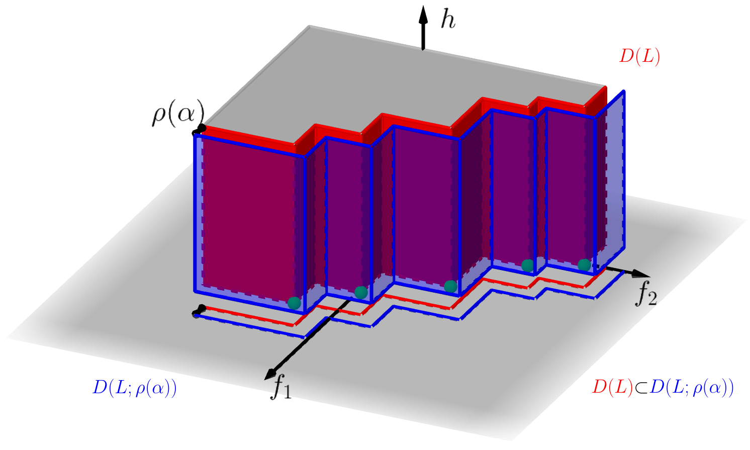
Figure 1: Globalization strategy based on a sufficient decrease condition in Algorithm 1.

The assumptions required to ensure globalization under a sufficient decrease approach are slightly different.

Assumption 3.8.

The function $F:\mathbb{R}^{n}\to\mathbb{R}^{m}$ is bounded in the set $\mathcal{S}:=\bigcup_{j=1}^{m}\{x\in X\mid h(x)\leq h_{\tt max}\wedge f_{j}(x)\leq f_{j}(x_{0})\}$.

By definition, $0\leq h(x)\leq h_{\tt max}$. Thus, Assumption 3.8 guarantees that the function $\bar{F}:\mathbb{R}^{n}\to\mathbb{R}^{m+1}$, defined by $\bar{F}=(F,h)$, is also bounded in $\mathcal{S}$.

The following theorem states the convergence to zero of at least one subsequence of step sizes, when using a globalization strategy based on sufficient decrease.

Theorem 3.9.

Consider a globalization strategy based on imposing a sufficient decrease condition and let Assumption 3.8 hold. Then, DMS-FILTER-IR generates a sequence of iterates satisfying

$$\liminf_{k\to+\infty}\alpha_{k}=0.$$

Proof.

Let us assume that $\displaystyle\liminf_{k\to+\infty}\alpha_{k}\neq 0$, meaning that there is $\alpha^{*}$ such that $\alpha_{k}>\alpha^{*}$ for all $k$. At each unsuccessful iteration $k$, the corresponding step size parameter is reduced by at least $\beta_{2}\in(0,1)$. Thus, the number of successful iterations must be infinite.

Successful iterations increase the hypervolume of the dominated region associated to the function $\bar{F}$ and the list of points in at least $(\rho(\alpha_{k}))^{m+1}$, where $\alpha_{k}$ represents the step size associated with the current iteration (see Lemma 3.1 in [20]).

Since $\rho(\cdot)$ is a nondecreasing function, which satisfies $\rho(t)>0$ for $t>0$, there exists $\rho^{*}>0$ such that $\rho(\alpha_{k})\geq\rho(\alpha^{*})=\rho^{*}$. Thus, any successful iteration will increase the hypervolume of the dominated region associated to the list of points for function $\bar{F}$ in at least $(\rho^{*})^{m+1}$, contradicting Assumption 3.8. ∎

3.2 Sequences and stationarity

To establish the convergence of direct search methods of directional type, the behavior of the algorithms needs to be analyzed at limit points of particular sequences of unsuccessful iterates, denoted by refining subsequences.

Definition 3.10.

A subsequence $\{x_{k}\}_{k\in K}$ of iterates generated by DMS-FILTER-IR, corresponding to unsuccessful poll steps, is said to be a refining subsequence if $\{\alpha_{k}\}_{k\in K}$ converges to zero.

Assumption 3.1, Theorems 3.6 or 3.9, and the updating strategy of the step size allow to establish the existence of at least one convergent refining subsequence (see, e.g., [19, Section 7.3]). The limit point $\bar{x}$ of a refining subsequence $\{x_{k}\}_{k\in K}$ is said to be a refined point. As suggested by the numerical experiments reported in Section 5, it is common that the algorithm will generate several refined points. In [10] the same type of result is established using the concept of linked sequences.

Refined points, corresponding to limit points of sequences of unsuccessful iterates, will be the natural candidates to Pareto-Clarke stationarity. For defining it, in a nonsmooth setting, we will need a generalization of the tangent cone commonly used in nonlinear programming, namely the Clarke’s tangent cone [17].

Definition 3.11.

A vector $d\in\mathbb{R}^{n}$ is said to be a Clarke tangent vector to the set $Y\subseteq\mathbb{R}^{n}$ at the point $\bar{x}\in cl(Y)$ if for every sequence $\{y_{k}\}$ of elements of $Y$ that converges to $\bar{x}$ and for every sequence of positive real numbers $\{t_{k}\}$ converging to zero, there exists a sequence of vectors $\{w_{k}\}$ converging to $d$ such that $y_{k}+t_{k}w_{k}\in Y$.

The set of all Clarke tangent vectors to $Y$ at $\bar{x}$ is called the Clarke tangent cone to $Y$ at $\bar{x}$, and is denoted by $T^{Cl}_{Y}(\bar{x})$. The tangent cone is the closure of another relevant cone for the following analysis, namely the Clarke’s hypertangent cone [17].

Definition 3.12.

A vector $d\in\mathbb{R}^{n}$ is said to be a Clarke hypertangent vector to the set $Y\subseteq\mathbb{R}^{n}$ at the point $\bar{x}\in Y$ if there exists a scalar $\epsilon>0$ such that $y+tw\in Y$ for all $y\in Y\cap B(\bar{x};\epsilon)$, $w\in B(d;\epsilon)$, and $0<t<\epsilon$.

The set of all hypertangent vectors to $Y$ at $\bar{x}$ is called the hypertangent cone to $Y$ at $\bar{x}$ and is denoted by $H^{Cl}_{Y}(\bar{x})$. Whenever the interior of $T^{Cl}_{Y}(\bar{x})$ is nonempty, $H^{Cl}_{Y}(\bar{x})=\operatorname{int}(T^{Cl}_{Y}(\bar{x}))$.

The notion of directional derivative needs also to be generalized to nonsmooth functions, accounting for the presence of constraints [17, 32].

Definition 3.13.

Let $g:\mathbb{R}^{n}\to\mathbb{R}$ be Lipschitz continuous near $\bar{x}\in Y$. The Clarke-Jahn generalized derivative of $g$ along $d\in H^{Cl}_{Y}(\bar{x})$ is defined as:

$$g^{\circ}(\bar{x};d):=\limsup_{x\to\bar{x},x\in Y\atop t\downarrow 0,x+td\in Y}\dfrac{g(x+td)-g(x)}{t}.$$

When $H^{Cl}_{Y}(\bar{x})$ is nonempty, the Clarke-Jahn generalized directional derivatives along directions $v$ in $T^{Cl}_{Y}(\bar{x})$ can be computed by taking limits of sequences of directions belonging to the hypertangent cone [6].

Proposition 3.14.

Let $g:\mathbb{R}^{n}\to\mathbb{R}$ be Lipschitz continuous near $\bar{x}\in Y$ and assume that $H^{Cl}_{Y}(\bar{x})$ is nonempty. The Clarke-Jahn generalized derivative of $g$ along $v\in T^{Cl}_{Y}(\bar{x})$ can be computed as:

$$g^{\circ}(\bar{x};v):=\lim_{d\to v\atop d\in H^{Cl}_{Y}(\bar{x})}g^{\circ}(\bar{x};d).$$

We are now in conditions of establishing what would be a first-order stationarity result for Problem (1). The following definition states essentially that there is no direction in the tangent cone that is descent for all components of the objective function.

Definition 3.15.

Let $F$ be Lipschitz continuous near a point $\bar{x}\in\Upsilon$. We say that $\bar{x}$ is a Pareto-Clarke critical point of $F$ in $\Upsilon$, if for each direction $d\in T^{Cl}_{\Upsilon}(\bar{x})$, there exists a $j=j(d)\in\{1,\ldots,m\}$ such that $f_{j}^{\circ}(\bar{x};d)\geq 0$.

If the objective function is differentiable, the previous definition can be reformulated using the columns of the Jacobian matrix.

Definition 3.16.

Let $F$ be strictly differentiable at a point $\bar{x}\in\Upsilon$. We say that $\bar{x}$ is a Pareto-Clarke-KKT critical point of $F$ in $\Upsilon$, if for each direction $d\in T_{\Upsilon}^{Cl}(\bar{x})$, there exists a $j=j(d)\in\{1,\ldots,m\}$ such that $\nabla f_{j}(x)^{\top}d\geq 0$.

Finally, for establishing the desired stationarity results we need the definition of refining directions associated with refined points.

Definition 3.17.

Let $\bar{x}$ be the limit point of a convergent refining subsequence $\{x_{k}\}_{k\in K}$. If the limit $\displaystyle\lim_{k\in K^{\prime}}\frac{d_{k}}{\|d_{k}\|}$ exists, where $K^{\prime}\subseteq K$ and $d_{k}\in D_{k}$, and if $x_{k}+\alpha_{k}d_{k}$ is feasible, for sufficiently large $k\in K^{\prime}$, then this limit is said to be a refining direction for $\bar{x}$.

The convergence analysis will initiate with the study of the behavior of the algorithm along refined directions, belonging to the hypertangent cone, both computed at a refined point.

3.3 DMS-FILTER-IR convergence results

In this section, we present the main convergence results of DMS-FILTER-IR. The analysis is based on the property established by Proposition 3.18, valid for any of the two globalization strategies considered. Function $\bar{\rho}(\cdot)$ corresponds to the forcing function $\rho(\cdot)$, when globalization is based on a sufficient decrease condition, or is defined as the null function ($\bar{\rho}(\cdot)=0$), when globalization results from the use of integer lattices. For simplicity when stating the results, we also define $f_{m+1}$ as being equal to $h$, the aggregated violation of the relaxed constraints.

Proposition 3.18.

Let $x\in L$ and $y\in\bar{X}$ be a dominated point at an iteration associated with the step size $\alpha$. Then:

$$\exists j\in\{1,\ldots,m+1\}:f_{j}(y)>f_{j}(x)-\bar{\rho}(\alpha).$$

Proof.

Point $y$ is dominated, meaning that there is $z\in L$ such that

$$\bar{F}(z)-\bar{\rho}(\alpha)\leq\bar{F}(y),$$

and, if $\bar{\rho}(\cdot)=0$, $\bar{F}(z)\neq\bar{F}(y)$.

Suppose $\bar{F}(x)-\bar{\rho}(\alpha)\geq\bar{F}(y)$. Then,

$$\bar{F}(x)\geq\bar{F}(x)-\bar{\rho}(\alpha)\geq\bar{F}(z)-\bar{\rho}(\alpha).$$

Moreover, if $\bar{\rho}(\cdot)=0$ then $\bar{F}(z)\neq\bar{F}(x)$. Thus, $x$ would be dominated by $z$, which is not possible, since both $x$ and $z$ belong to the list of nondominated points $L$. ∎

As the step size approaches zero, the poll step will allow to recover the local sensitivities of the objective function. Together with some proper smoothness assumptions, we can establish that there is no locally improving direction, for the adequate problem. The proof follows directly from Theorem 4.8 in [21]. For completeness, we reproduce it in Theorem 3.19, with the due adaptations.

Theorem 3.19.

Consider $\{x_{k}\}_{k\in K}$, a refining subsequence generated by DMS-FILTER-IR, converging to the refined point $\bar{x}\in\bar{X}$. Assume that $\bar{F}$ is Lipschitz continuous near $\bar{x}$. Let $d\in H^{Cl}_{\bar{X}}(\bar{x})$ be a refining direction for $\bar{x}$, associated with the refining subsequence $\{x_{k}\}_{k\in K}$. Then,

$$\exists j\in\{1,\ldots,m+1\}:f_{j}^{\circ}(\bar{x};d)\geq 0.$$

Proof.

Since $\{x_{k}\}_{k\in K}$ is a refining subsequence converging to $\bar{x}$, we have $\lim_{k\in K}x_{k}=\bar{x}$, $\lim_{k\in K}\alpha_{k}=0$ and $k\in K$ is the index of an unsuccessful iteration.

Consider $K^{\prime}\subseteq K$ such that $\lim_{k\in K^{\prime}}\frac{d_{k}}{\|d_{k}\|}=d\in H_{\bar{X}}^{Cl}(\bar{x})$, with $d_{k}$ a poll direction used at iteration $k$. Let $j\in\{1,\ldots,m+1\}$. Then,

$$f_{j}^{\circ}(\bar{x};d)=\limsup_{x\rightarrow\bar{x},x\in\bar{X}\atop t\downarrow 0,x+td\in\bar{X}}\dfrac{f_{j}(x+td)-f_{j}(x)}{t}\geq\limsup_{k\in K^{\prime}}\dfrac{f_{j}(x_{k}+\alpha_{k}\|d_{k}\|d)-f_{j}(x_{k})}{\alpha_{k}\|d_{k}\|}=$$

$$=\limsup_{k\in K^{\prime}}\left(\dfrac{f_{j}(x_{k}+\alpha_{k}d_{k})-f_{j}(x_{k})+\bar{\rho}(\alpha_{k})}{\alpha_{k}\|d_{k}\|}+\dfrac{f_{j}(x_{k}+\alpha_{k}\|d_{k}\|d)-f_{j}(x_{k}+\alpha_{k}d_{k})}{\alpha_{k}\|d_{k}\|}-\frac{\bar{\rho}(\alpha_{k})}{\alpha_{k}\|d_{k}\|}\right)\geq$$

$$\geq\limsup_{k\in K^{\prime}}\dfrac{f_{j}(x_{k}+\alpha_{k}d_{k})-f_{j}(x_{k})+\bar{\rho}(\alpha_{k})}{\alpha_{k}\|d_{k}\|}+\liminf_{k\in K^{\prime}}\left(\dfrac{f_{j}(x_{k}+\alpha_{k}\|d_{k}\|d)-f_{j}(x_{k}+\alpha_{k}d_{k})}{\alpha_{k}\|d_{k}\|}-\frac{\bar{\rho}(\alpha_{k})}{\alpha_{k}\|d_{k}\|}\right)$$

Since each $d_{k}$ is lower bounded by $d_{min}>0$, the definition of $\bar{\rho}(\cdot)$ and the properties of the forcing function, allow to establish $\lim_{k\in K^{\prime}}\frac{\bar{\rho}(\alpha_{k})}{\alpha_{k}\|d_{k}\|}=0$.

Moreover, the Lipschitz continuity of $\bar{F}$ ensures that

$$\left|\dfrac{f_{j}(x_{k}+\alpha_{k}\|d_{k}\|d)-f_{j}(x_{k}+\alpha_{k}d_{k})}{\alpha_{k}\|d_{k}\|}\right|\leq L\left\|d-\frac{d_{k}}{\|d_{k}\|}\right\|,$$

where $L$ represents the maximum of the Lipschitz constants associated to each one of the objective function components. Thus, the fact that $\lim_{k\in K^{\prime}}\frac{d_{k}}{\|d_{k}\|}=d$ ensures that

$$\lim_{k\in K^{\prime}}\dfrac{f_{j}(x_{k}+\alpha_{k}\|d_{k}\|d)-f_{j}(x_{k}+\alpha_{k}d_{k})}{\alpha_{k}\|d_{k}\|}=0.$$

We then have,

$$f_{j}^{\circ}(\bar{x};d)\geq\limsup_{k\in K^{\prime}}\dfrac{f_{j}(x_{k}+\alpha_{k}d_{k})-f_{j}(x_{k})+\bar{\rho}(\alpha_{k})}{\alpha_{k}\|d_{k}\|}.$$

Now, $k\in K^{\prime}$ is an unsuccessful iteration and $x_{k}\in L$. By Proposition 3.18,

$$\exists j(k)\in\{1,\ldots,m+1\}:f_{j(k)}(x_{k}+\alpha_{k}d_{k})>f(x_{k})-\bar{\rho}(\alpha_{k}).$$ (6)

Since the number of components of the objective function is finite, by passing to a subsequence $K^{\prime\prime}\subseteq K^{\prime}$ that always uses the same component of $\bar{F}$ we have the desired result. ∎

The convergence to Pareto-Clarke or Pareto-Clarke-KKT critical points can be proven by imposing asymptotic density in the unit sphere of the set of refining directions associated with $\bar{x}$.

Theorem 3.20.

Consider $\{x_{k}\}_{k\in K}$, a refining subsequence generated by DMS-FILTER-IR, converging to the refined point $\bar{x}\in\bar{X}$. Assume that $H_{\bar{X}}^{Cl}(\bar{x})\neq\emptyset$ and that $\bar{F}$ is Lipschitz continuous near $\bar{x}$. If the set of refining directions for $\bar{x}$ is dense in $T^{Cl}_{\bar{X}}(\bar{x})$, then $\bar{x}$ is a Pareto-Clarke critical point for Problem (5). If, in addition, $F$ is strictly differentiable at $\bar{x}$, then this point is a Pareto-Clarke-KKT critical point for Problem (5).

Proof.

The proof follows from Theorem 3.19, using similar arguments to the ones of Theorem 4.9 in [21]. ∎

The previous theorem states that DMS-FILTER-IR generates a Pareto-Clarke critical point for Problem (5). However, if $\bar{x}$ is a local efficient point of Problem (5) and $h(\bar{x})=0$, then $\bar{x}$ is a local efficient point for Problem (1).

Thus, a question that arises is if the algorithm is indeed able to generate feasible points, when initialized from infeasible ones. The next theorem attempts to establish some conditions that provide an answer to this question.

Theorem 3.21.

Let Assumption 3.1 hold. Assume that $h$ is a continuous function and consider $\{x_{k}\}_{k\in K}$, an infeasible refining subsequence, such that for each $k\in K$, $x_{k}$ is used at a successful inexact restoration step in DMS-FILTER-IR. Then, the algorithm generates a limit point $\bar{y}\in\Upsilon$.

Proof.

For each $k\in K$, $x_{k}$ was used at a successful inexact restoration step. Thus, there is $y_{k}^{*}\in X$ such that $y_{k}^{*}$ is nondominated and $0\leq h(y_{k}^{*})\leq\xi(\alpha_{k})h(x_{k})\leq h_{\tt max}$.

Since $\{x_{k}\}_{k\in K}$ is a refining subsequence, $\lim_{k\in K}\alpha_{k}=0$. Considering the properties of $\xi(\cdot)$ and the boundedness of $h$, we can conclude $\lim_{k\in K}h(y_{k}^{*})=0$. Assumption 3.1 allows to consider $K^{\prime}\subseteq K$ such that $\lim_{k\in K}y_{k}^{*}=\bar{y}$ and the continuity of $h$ establishes $h(\bar{y})=0$, meaning that $\bar{y}\in\Upsilon$. ∎

The following result links sequences of points generated by DMS-FILTER-IR to Problem (1). For establishing it, we will assume that globalization is based on the use of integer lattices.

Corollary 3.22.

Consider $\{x_{k}\}_{k\in K}$ a feasible refining subsequence, converging to the refined point $\bar{x}\in\Upsilon$, generated by algorithm DMS-FILTER-IR, when using a globalization strategy based on integer lattices. Assume that $\bar{F}$ is Lipschitz continuous near $\bar{x}$. Let $d\in H^{Cl}_{\Upsilon}(\bar{x})$ be a refining direction for $\bar{x}$, associated with the refining subsequence $\{x_{k}\}_{k\in K}$. Then,

$$\exists j\in\{1,\ldots,m\}:f_{j}^{\circ}(\bar{x};d)\geq 0.$$

Proof.

The proof follows directly from the proof of Theorem 3.19, considering $d\in H^{Cl}_{\Upsilon}(\bar{x})$ and noting that for $k$ sufficiently large $h(x_{k}+\alpha_{k}d_{k})=0=h(x_{k})$. Thus, inequality (6) needs to hold for $j\in\{1,\ldots,m\}$. ∎

In this situation, $\bar{x}$ is a Pareto-Clark critical point for Problem (1).

Corollary 3.23.

Consider $\{x_{k}\}_{k\in K}$, a feasible refining subsequence generated by DMS-FILTER-IR, converging to the refined point $\bar{x}\in\Upsilon$. Assume that $H_{\Upsilon}^{Cl}(\bar{x})\neq\emptyset$ and that $\bar{F}$ is Lipschitz continuous near $\bar{x}$. If the set of refining directions for $\bar{x}$ is dense in $T^{Cl}_{\Upsilon}(\bar{x})$, then $\bar{x}$ is a Pareto-Clarke critical point for Problem (1). If, in addition, $F$ is strictly differentiable at $\bar{x}$, then this point is a Pareto-Clarke-KKT critical point for Problem (1).

Proof.

The proof is a direct consequence of Corollary 3.22, using similar arguments to the ones of Theorem 4.9 in [21]. ∎

By using a filter-based approach, we have overcome the difficulty of applying directional direct search to multiobjective constrained optimization problems, when a feasible initialization is not available (regarding the relaxable constraints). The incorporation of a inexact restoration step potentiates feasibility. The next section will illustrate the numerical competitiveness of the proposed approach.

4 Implementation Details

Differently from DMulti-MADS-PB [11], DMS-FILTER-IR selects a single point at each iteration, to be explored at the search and, possibly, at the inexact restoration and/or pool steps. The decision on using a feasible or infeasible iterate point always attempts to promote feasibility, regarding the relaxable constraints (unrelaxable constraints are always satisfied by the points in the list, from where the iterate point will be selected).

The algorithm switches to an infeasible iterate point if the current feasible iterate point only generates infeasible points. At the next iteration, the iterate point will be selected from the nondominated points in the list that do not satisfy the relaxable constraints. Once that an infeasible iterate point generates at least one feasible point, a feasible point will be selected as iterate point for the next iteration.

Suppose that we are at one iteration where the iterate point should be feasible. For selecting it from all the feasible points in the iterate list, we use the concept of the most isolated point. For each component of the objective function $i=1,\ldots,m$, the feasible points in $L_{k}$ are selected and ordered by increasing function value:

$$f_{i}(x^{1})\leq f_{i}(x^{2})\leq\ldots\leq f_{i}(x^{m_{F}}),$$

where $m_{F}$ denotes the total number of feasible points in $L_{k}$.

Then, for each component of the objective function $f_{i}$, $i=1,\ldots,m$, and for each feasible point $x^{j}$ in $L_{k}$, with $j=1,\ldots,m_{F}$, the following indicator is computed:

$$\delta_{i}\left(x^{j}\right)=\begin{cases}f_{i}\left(x^{2}\right)-f_{i}\left(x^{1}\right)&\text{, if }j=1\\ f_{i}\left(x^{m_{F}}\right)-f_{i}\left(x^{m_{F}-1}\right)&\text{, if }j=m_{F}\\ \dfrac{f_{i}\left(x^{j+1}\right)-f_{i}\left(x^{j-1}\right)}{2}&\text{, otherwise. }\end{cases}$$

The most isolated point corresponds to the maximum value of $\gamma_{j}$, that is,

$$x_{k}\in\displaystyle\operatorname*{argmax}_{j=1,\ldots,m_{F}}\gamma_{j},$$

where

$$\gamma_{j}=\displaystyle\dfrac{1}{m}\sum_{i=1}^{m}\delta_{i}(x^{j}).$$ (7)

When the iterate point should be infeasible, two different criteria are used for its selection, depending on having at least one feasible point in the list or not. In the latter situation, the point selected corresponds to the most promising infeasible point is the list, in terms of restoring the feasibility. Thus, the point with the smallest value for the aggregated constraint violation function $h$ will be chosen.

Now, suppose that there is at least one feasible point in the list. The fact that the iterate point should be infeasible means that at the last iteration a feasible iterate point only generated infeasible ones. Thus, we want to try to restore feasibility close to the region that was being explored. A closed ball centered on the feasible iterate point, of radius equal to $\eta\,\alpha_{k}\max_{d\in D_{k-1}}\|d\|$, with $\eta\geq\frac{1}{\beta_{2}}$, is considered and the infeasible point in the list, belonging to this ball, with the lowest value for the aggregated constraint violation function $h$ will be selected as iterate point.

DMS-FILTER-IR was implemented in Matlab, keeping the default settings of DMS. Thus, the step size was initialized as $1$, kept constant at successful iterations ($\gamma=1$), and halved at unsuccessful ones ($\beta_{1}=\beta_{2}=0.5$). No search step was implemented.

The aggregated violation function was defined as:

$$h(x)=\|C(x)_{+}\|_{2}^{2}=\displaystyle\sum_{i=1}^{p}\max\{0,c_{i}(x)\}^{2}.$$

Regarding the maximum violation allowed, $h_{\tt max}$, it depends on the initialization. If there are any infeasible points in the list, $h_{\tt max}$ will be set equal to the largest of the existing values of $h$. Otherwise, it will be set equal to the maximum between $10$ and half of the number of the relaxable constraints.

Many options can be considered for defining a function complying with the requirements of $\xi(\cdot)$, to be used in the inexact restoration step. In the numerical implementation, we used the function $\xi(\alpha)=(\frac{\alpha}{2})^{2}$. Note that this function is continuous, $\xi(\alpha)\to 0$ when $\alpha\downarrow 0$ and, considering the initialization and the strategy to update the step size, $0<\xi(\alpha)<1$. The inexact restoration problems were solved with the Matlab function fmincon.m. Through the numerical section, for any solver, feasibility is assumed to be achieved when there is an aggregated violation of the relaxable constraints less than $10^{-5}$.

If the poll step is performed, a complete polling approach is adopted, evaluating all the points corresponding to directions in the positive spanning set.

5 Numerical Experiments

This section is devoted to the numerical experiments performed with DMS-FILTER-IR, illustrating its numerical behavior by comparison with the original DMS algorithm, when solving constrained problems, or with other state-of-art solvers. A first subsection will describe the metrics used in the performance assessment, followed by a new subsection detailing the problem collection. The last two subsections illustrate the numerical behavior of the proposed algorithm. All tests were performed in a laptop with a 11th Gen Intel® Core(TM) i7-1165G7 processor, at 2.80GHz, with 16GB of RAM memory, using Windows 11 with 64 bits.

5.1 Performance Assessment

In order to evaluate the numerical performance of the algorithm, we resource to performance profiles, a tool introduced by Dolan and Moré [24], for single objective nonlinear optimization. This tool allows to concurrently assess the numerical performance of multiple solvers, for different metrics. The performance of a solver $s$, belonging to a set of solvers $S$, on a particular set of problems $P$ is represented by the cumulative function:

$$\rho_{s}(\tau)=\dfrac{1}{|P|}\left|\left\{p\in P\mid t_{p,s}\leq\tau\min\{t_{p,s}:s\in S\}\right\}\right|,$$

where $\tau\geq 1$ and $t_{p,s}$ represents the value of the selected metric, obtained by solver $s\in S$ on problem $p\in P$. It is assumed that lower values of $t_{p,s}$ correspond to a better values for the metric.

Higher values of $\rho_{s}(\tau)$ represent a better numerical performance for solver $s$. Specifically, the solver with the highest $\rho_{s}(1)$ value is considered the most efficient and the solver with the greatest $\rho_{s}(\tau)$ value for large values of $\tau$ is regarded as the most robust.

As metrics, purity, hypervolume, and the spread metrics $\Gamma$ and $\Delta$ were selected. The percentage of nondominated points generated by a given solver is measured by purity:

$$\bar{t}_{p,s}={Pur}_{p,s}=\frac{|F_{p,s}\cap F_{p}|}{|F_{p,s}|},$$

where $F_{p,s}$ represents the approximation to the Pareto front of problem $p$ computed by solver $s$ and $F_{p}$ is a reference Pareto front for problem $p$, computed by considering the union of the Pareto approximations corresponding to all solvers, $\cup_{s\in S}F_{p,s}$, and removing from it all the dominated points [21].

Hypervolume [47], additionally to nondominance, encompasses the notion of spread by quantifying the volume of the region dominated by the current approximation of the Pareto front and limited by a reference point $U_{p}\in\mathbb{R}^{m}$, dominated by all points belonging to the different approximations computed for the Pareto front of problem $p\in P$ by all solvers tested. In a formal way:

$$\bar{t}_{p,s}=HV_{p,s}=Vol\{y\in\mathbb{R}^{m}\,|\,y\leq U_{p}\wedge\exists x\in F_{p,s}:x\leq y\}=Vol\left(\bigcup_{x\in F_{p,s}}[x,U_{p}]\right),$$

where $Vol(.)$ denotes the Lebesgue measure of a $m$-dimensional set of points and $[x,U_{p}]$ denotes the interval box with lower corner $x$ and upper corner $U_{p}$.

Since larger values of purity and hypervolume indicate a better performance, the inverse value of each one of the metrics was used ($t_{p,s}=1/\bar{t}_{p,s}$), when computing the associated performance profiles.

Lastly, for a direct evaluation of spread along the Pareto front, we incorporated two supplementary metrics: the $\Gamma$ metric, quantifying the magnitude of the largest gap in the computed Pareto front approximation, and the $\Delta$ metric, which gauges the evenness of the distribution of nondominated points within the generated approximation.

Consider that solver $s\in S$ computed for problem $p\in P$ an approximation to the Pareto front with points $x^{1},x^{2},\ldots,x^{N}$, to which we add the so-called extreme points, $x^{0}$ and $x^{N+1}$, corresponding to the points with the best and worst values for each component of the objective function. The metric $\Gamma$ can be computed as:

$$\Gamma_{p,s}\;=\;\max_{j\in\{1,\dots,q\}}\left(\max_{i\in\{0,\dots,N\}}\{\delta_{j,i}\}\right),$$ (8)

where $\delta_{j,i}=f_{j}(x^{i+1})-f_{j}(x^{i})$, assuming that the objective function values have been sorted by increasing order for each objective function component $j$. The metric $\Delta$ [22] is computed as:

$$\Delta_{p,s}\;=\;\max_{j\in\{1,\dots,q\}}\left(\frac{\delta_{j,0}+\delta_{j,N}+\sum_{i=1}^{N-1}|\delta_{j,i}-\bar{\delta}_{j}|}{\delta_{j,0}+\delta_{j,N}+(N-1)\bar{\delta}_{j}}\right),$$ (9)

where $\bar{\delta}_{j}$, for $j=1,\ldots,q$, represents the average of the distances $\delta_{j,i}$, $i=1,\dots,N-1$.

5.2 Problem Collection

Liuzzi et al. [37] defined a collection of constrained problems by coupling a subset of the bound constrained problems provided in Custódio et al. [21] with six families of constraints proposed in [33]. All the bound problems in [21] with $n\geq 3$ variables were selected, resulting in $51$ bound constrained problems. A set of $306$ constrained problems was generated by adding to each problem the following six families of nonlinear constraints (the suggested initialization is denoted by $x^{0}$):

$$g_{j}^{1}(x) = (3-2x_{j+1})x_{j+1}-x_{j}-2x_{j+2}+1,\quad j=1,\ldots,p,\quad p=n-2$$

$$x^{0}_{i}=1,\quad i=1,\ldots,n$$

$$g_{j}^{2}(x) = (3-2x_{j+1})x_{j+1}-x_{j}-2x_{j+2}+2.5,\quad j=1,\ldots,p,\quad p=n-2$$

$$x^{0}_{i}=2,\quad i=1,\ldots,n$$

$$g_{j}^{3}(x) = x_{j}^{2}+x_{j+1}^{2}+x_{j}x_{j+1}-2x_{j}-2x_{j+1}+1,\quad j=1,\ldots,p,\quad p=n-1$$

$$x^{0}_{i}=0.5\quad i=1,\ldots,n$$

$$g_{j}^{4}(x) = x_{j}^{2}+x_{j+1}^{2}+x_{j}x_{j+1}-1,\quad j=1,\ldots,p,\quad p=n-1$$

$$x^{0}_{i}=0,\quad i=1,\ldots,n$$

$$g_{j}^{5}(x) = (3-0.5x_{j+1})x_{j+1}-x_{j}-2x_{j+2}+1,\quad j=1,\ldots,p,\quad p=n-2,$$

$$x^{0}_{i}=2,\quad i=1,\ldots,n$$

$$g_{j}^{6}(x) = \displaystyle\sum_{i=1}^{n-2}((3-0.50x_{i+1})x_{i+1}-x_{i}-2x_{i+2}+1),\quad j=p,\quad p=1$$

$$x^{0}_{i}=2,\quad i=1,\ldots,n$$

In theory, DMS is developed for multiobjective derivative-free optimization, regardless of the number of components in the objective function. However, the numerical results reported in [21] respect to biojective and triobjective problems (there is an exception of one problem with four components in the objective function, from the set of 100 bound constrained problems considered). In fact, it is common knowledge in the multiobjective optimization community that addressing problems with more than three components in the objective function requires special techniques, falling on the specific domain of Many-objective Optimization [27]. The focus of this work is not Many-objective Optimization problems. Considering that the aggregated penalization function will be an additional component of the objective function, we restricted the set of $306$ constrained problems to biobjective ones, in a total of $156$. The problems and their dimensions are given in Table 1.

Problem	n	Problem	n	Problem	n
CL1	4	L2ZDT6	10	QV1	10
DPAM1	10	L3ZDT1	30	ZDT1	30
FES1	10	L3ZDT2	30	ZDT2	30
Kursawe	3	L3ZDT3	30	ZDT3	30
L1ZDT4	10	L3ZDT4	30	ZDT4	10
L2ZDT1	30	L3ZDT6	10	ZDT6	10
L2ZDT2	30	MOP2	4	SK2	4
L2ZDT3	30	MOP4	3	TKLY1	4
L2ZDT4	30	OKA2	3

Table 1: The biobjective test set used in the numerical experiments ($n$ denotes the number of variables).

DMS requires a feasible initialization. However, not all the points $x^{0}$ provided by Karmitsa [33] satisfy the bounds constraints. Thus, from the $156$ biobjective problems considered, we retained only the $93$ for which a feasible initialization was available. The final test set comprise $93$ nonlinearly constrained biobjective problems, with $n\in[3,30]$ and $p\in[1,29]$. We assumed the nonlinear constraints as being relaxable, corresponding the unrelaxable constraints to bounds.

5.3 Positive Spanning Sets

The convergence of both DMS and DMS-FILTER-IR is established under the assumption of asymptotic density of the sets of directions used by the algorithm, during the optimization process. However, when the budget of function evaluations is limited, which is often the case when the function is expensive to evaluate, this density is never accomplished. Coordinate search has the perfect geometry for bound constrained problems. In fact, this was the type of directions used to obtain the numerical results reported in [21], illustrating the numerical performance of DMS.

Considering that in DMS-FILTER-IR the nonlinear constraints are addressed by the filter approach, using the aggregated violation function and reducing the problem to a bound constrained problem, it would be interesting to compare DMS and DMS-FILTER-IR when using coordinate search as set of directions or when resorting to an asymptotic dense set of directions, built using the technique proposed in [1], based on Halton sequences.

DMS addresses constraints with an extreme barrier approach, denoted here by DMS-EB, only evaluating feasible points and requiring a feasible initialization. Thus, the feasible point $x^{0}$ given in [33] was used for initialization. DMS-FILTER-IR allows infeasible points, with respect to the relaxable constraints. Therefore, DMS-FILTER-IR was initialized with $n$-points equally spaced in the line segment, joining the variable upper and lower bounds.

Figures 2 and 3 report the results obtained for DMS and DMS-FILTER-IR, respectively. A maximum budget of $5000$ function evaluations was allowed, jointly with a minimum step size of $10^{-3}$, for all the points in the list.

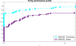
(a) Purity

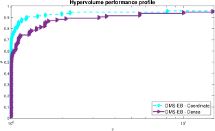
(b) Hypervolume

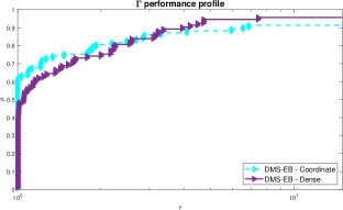
(c) Spread Gamma

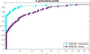
(d) Spread Delta

Figure 2: Performance profiles for DMS considering different types of positive spanning sets and a maximum budget of $5000$ function evaluations.

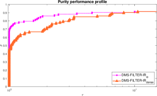
(a) Purity

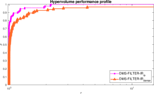
(b) Hypervolume

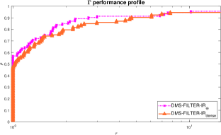
(c) Spread Gamma

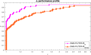
(d) Spread Delta

Figure 3: Performance profiles for DMS-FILTER-IR considering different types of positive spanning sets and a maximum budget of $5000$ function evaluations.

With exception to the spread metric $\Gamma$, where the results are very close, for any of the metrics considered, it is clear the advantage of the use of coordinate directions as positive spanning set, both for DMS and DMS-FILTER-IR. As already mentioned, this could be the result of the nice geometry associated to these directions and bound constrained problems. Thus, in the next section, DMS and DMS-FILTER-IR will consider positive spanning sets based on coordinate search.

5.4 Comparison With Other Solvers

In addition to DMS [21], DFMO [37], and DMultiMADS-PB [11] were also tested as benchmark solvers to evaluate the performance of DMS-FILTER-IR. The DMS solver is implemented in Matlab and is freely available at http://www.mat.uc.pt/dms. DFMO is coded in Fortran90 and is available at http://www.dis.uniroma1.it/~lucidi/DFL. Finally, coded in Julia, DMultiMADS-PB can be obtained from https://github.com/bbopt/DMultiMadsPB.

The DFMO and DMultiMADS-PB algorithms address nonlinearly constrained multiobjective optimization problems by penalizing the nonlinear constraints with an exact merit function or by using a progressive barrier approach, respectively. As already mentioned, DMS addresses constraints with an extreme barrier function.

All solvers were run with the defaults, selecting the best version identified in [37] for DFMO and using the best version reported in [11] for DMultiMADS-PB. Results were obtained for maximum budgets of $500$ and $5000$ function evaluations. Considering the expensive nature of the function evaluation, small budgets are particular relevant for evaluating the performance of the solvers.

As in the previous subsection, DMS-EB was initialized with the feasible point $x^{0}$ provided in [33]. DMS-FILTER-IR, DMultiMADS-PB, and DFMO can be initialized with infeasible points. Therefore, DMS-FILTER-IR and DMultiMADS-PB were initialized with $n$-points equally spaced in the line segment, joining the variable upper and lower bounds, which is the default initialization of DMultiMADS-PB. DFMO was initialized with the centroid of the box defined by the bound constraints. After, the algorithm also generates $n$-points equally spaced in the line segment joining the bounds.

Figure 4 depicts performance profiles for the different metrics considered, when a maximum budget of $500$ function evaluations is allowed.

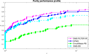
(a) Purity

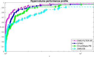
(b) Hypervolume

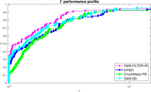
(c) Spread Gamma

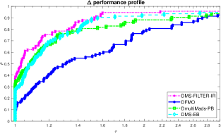
(d) Spread Delta

Figure 4: Comparing DMS-FILTER-IR with DFMO, DMultiMADS-PB, and DMS based on performance profiles for a maximum of $500$ function evaluations.

In general, DMS-FILTER-IR presents a good performance for any of the four metrics considered. Noteworthy, it is the most efficient solver for hypervolume and presents some advantage regarding robustness for the purity metric.

When the maximum budget allowed increases to $5000$ function evaluations (see Figure 5), DMS-FILTER-IR remains as the most competitive solver in what respects purity and hypervolume. For the spread metric $\Delta$, DMS-EB presents a better performance. DFMO provides some good results in terms of the largest gap in the Pareto front, represented by metric $\Gamma$.

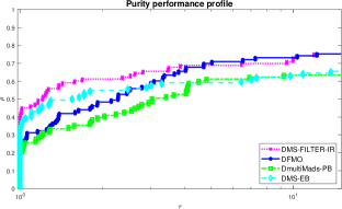
(a) Purity

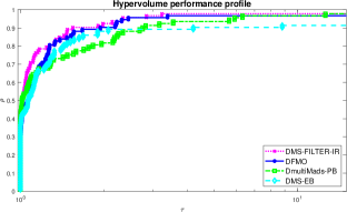
(b) Hypervolume

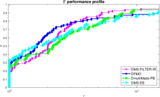
(c) Spread Gamma

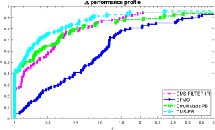
(d) Spread Delta

Figure 5: Comparing DMS-FILTER-IR with DFMO, DMultiMads-PB, and DMS based on performance profiles for a maximum of $5000$ function evaluations.

Individual comparisons between DMS-FILTER-IR and each of the three remaining solvers considered can be found in Figures 6 and 7, for budgets of $500$ and $5000$ function evaluations, respectively, clarifying the previous analysis and supporting the conclusions drawn.

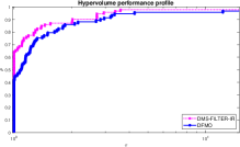
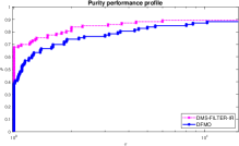
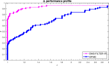
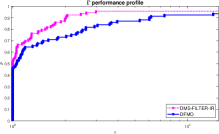
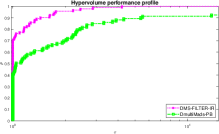
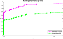
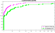
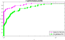
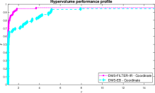
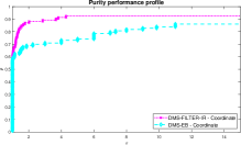
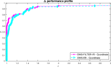
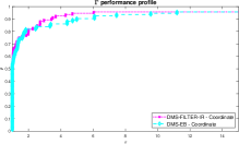
Figure 6: Individual comparison between DMS-FILTER-IR and DFMO, DMultiMADS-PB, and DMS based on performance profiles for a maximum budget of $500$ function evaluations.

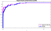
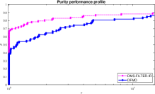
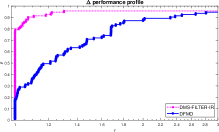
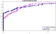
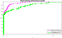
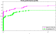
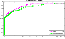
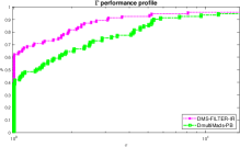
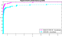
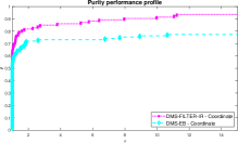
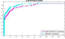
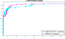
Figure 7: Individual comparison between DMS-FILTER-IR and DFMO, DMultiMADS-PB, and DMS based on performance profiles for a maximum budget of $5000$ function evaluations.

6 Conclusions

In this paper, we introduced, analyzed, and tested a filter-based derivative-free approach, using an inexact restoration step, for constrained multiobjective optimization problems. The DMS-FILTER-IR algorithm is able to address multiobjective derivative-free optimization problems without a feasible initialization, regarding the relaxable constraints.

Under the common assumptions used in derivative-free optimization analysis, we could establish the existence of at least one sequence of iterates generated by the algorithm that converges to a Pareto-Clarke critical point of a related problem. Additional conditions were provided that ensure the existence of a feasible point and the convergence to a Pareto-Clarke critical point of the original problem.

Extensive numerical experience allowed to establish the competitiveness of the proposed algorithm, by comparison with state-of-art solvers for multiobjective derivative-free constrained optimization. Filter methods combined with inexact restoration techniques are a valuable alternative to penalty function methods or the use of a progressive barrier strategy.

Several extensions can be considered to improve the numerical performance of DMS-FILTER-IR, namely the definition of a search step, based on surrogate models [14] or the use of parallelism [44]. Moreover, techniques from many-objective optimization literature can allow the development of efficient numerical implementations of DMS-FILTER-IR to address problems with more than two components in the objective function.

References

- [1] M. A. Abramson, C. Audet, J. E. Dennis, Jr., and S. Le Digabel. OrthoMADS: A deterministic MADS instance with orthogonal directions. SIAM J. Optim., 20:948–966, 2009.
- [2] R. Andreani, A. L. Custódio, and M. Raydan. Using first-order information in direct multisearch for multiobjective optimization. Optim. Methods Softw., 37:2135–2156, 2022.
- [3] M. B. Arouxét, N. E. Echebest, and E. A. Pilotta. Inexact restoration method for nonlinear optimization without derivatives. J. Comput. Appl. Math., 290:26–43, 2015.
- [4] C. Audet and W. Hare. Derivative-Free and Blackbox Optimization. Springer, Cham, Switzerland, 2017.
- [5] C. Audet and J. E. D. Jr. A pattern search filter method for nonlinear programming without derivatives. SIAM J. Optim., 14:980–1010, 2004.
- [6] C. Audet and J. E. D. Jr. Mesh adaptive direct search algorithms for constrained optimization. SIAM J. Optim., 17:188–217, 2006.
- [7] C. Audet and J. E. Dennis Jr. A progressive barrier for derivative-free nonlinear programming. SIAM J. Optim., 20:445–472, 2009.
- [8] C. Audet, G. Savard, and W. Zghal. Multiobjective optimization through a series of single-objective formulations. SIAM J. Optim., 19:188–210, 2008.
- [9] C. Audet, G. Savard, and W. Zghal. A mesh adaptive direct search algorithm for multiobjective optimization. European J. Oper. Res., 204:545–556, 2010.
- [10] J. Bigeon, S. L. Digabel, and L. Salomon. Dmulti-mads: mesh adaptive direct multisearch for bound-constrained blackbox multiobjective optimization. Comput. Optim. Appl., 79:301–338, 2021.
- [11] J. Bigeon, S. L. Digabel, and L. Salomon. Handling of constraints in multiobjective blackbox optimization, 2022.
- [12] E. G. Birgin, N. Krejić, and J. M. Martínez. Inexact restoration for derivative-free expensive function minimization and applications. J. Comput. Appl. Math., 410:114193, 2022.
- [13] J. Branke, K. Deb, K. Miettinen, and R. Slowiński, editors. Multiobjective Optimization: Interactive and Evolutionary Approaches. Springer-Verlag, Berlin, Germany, 2008.
- [14] C. P. Brás and A. L. Custódio. On the use of polynomial models in multiobjective directional direct search. Comput. Optim. Appl., 77:897–918, 2020.
- [15] R. P. Brito and P. Júdice. Asset classification under the ifrs 9 framework for the construction of a banking investment portfolio. Int. Trans. in Oper. Res., 29:2613–2648, 2022.
- [16] L. F. Bueno, A. Friedlander, J. M. Martínez, and F. N. C. Sobral. Inexact restoration method for derivative-free optimization with smooth constraints. SIAM J. Optim., 23:1189–1213, 2013.
- [17] F. H. Clarke. Optimization and Nonsmooth Analysis. SIAM, Philadelphia, USA, 1990.
- [18] G. Cocchi, G. Liuzzi, A. Papini, and M. Sciandrone. An implicit filtering algorithm for derivative-free multiobjective optimization with box constraints. Comput. Optim. Appl., 69:267–296, 2018.
- [19] A. R. Conn, K. Scheinberg, and L. N. Vicente. Introduction to Derivative-Free Optimization. MPS-SIAM Series on Optimization. SIAM, Philadelphia, USA, 2009.
- [20] A. L. Custódio, Y. Diouane, R. Garmanjani, and E. Riccietti. Worst-case complexity bounds of directional direct-search methods for multiobjective optimization. J. Optim. Theory Appl., 188:73–93, 2021.
- [21] A. L. Custódio, J. F. A. Madeira, A. I. F. Vaz, and L. N. Vicente. Direct multisearch for multiobjective optimization. SIAM J. Optim., 21:1109–1140, 2011.
- [22] K. Deb, A. Pratap, S. Agarwal, and T. Meyarivan. A fast and elitist multiobjective genetic algorithm: NSGA-II. IEEE T. Evolut. Comput., 6:182–197, 2002.
- [23] S. Deshpande, L. T. Watson, and R. A. Canfield. Multiobjective optimization using an adaptive weighting scheme. Optim. Methods Softw., 31:110–133, 2016.
- [24] E. D. Dolan and J. J. Moré. Benchmarking optimization software with performance profiles. Math. Program., 91:201–213, 2002.
- [25] N. Echebest, M. L. Schuverdt, and R. P. Vignau. An inexact restoration derivative-free filter method for nonlinear programming. Comp. and Appl. Math., 36:693–718, 2017.
- [26] G. Eichfelder. Adaptive Scalarization Methods in Multiobjective Optimization. Vector Optimization. Springer, Heidelberg, Germany, 2008.
- [27] M. T. M. Emmerich and A. H. Deutz. A tutorial on multiobjective optimization: fundamentals and evolutionary methods. Nat. Computing, 17:585–609, 2018.
- [28] P. S. Ferreira, E. W. Karas, M. Sachine, and F. N. Sobral. Global convergence of a derivative-free inexact restoration filter algorithm for nonlinear programming. Optim., 66:271–292, 2017.
- [29] R. Fletcher and S. Leyffer. Nonlinear programming without a penalty function. Math. Program., 91:239–269, 2002.
- [30] R. Fletcher, S. Leyffer, and P. L. Toint. A brief history of filter methods. SIAG/OPT Views-and-News, 18:2–12, 2007.
- [31] A. Habib, A. P. Butler, J. P. Bloomfield, and J. P. R. Sorensen. Fractal domain refinement of models simulating hydrological time series. Hydrological Sci. J., 67:1342–1355, 2022.
- [32] J. Jahn. Introduction to the Theory of Nonlinear Optimization. Springer-Verlag, Berlin, Germany, 1996.
- [33] N. Karmitsa. Test problems for large-scale nonsmooth minimization. Reports of the Department of Mathematical Information Technology 4, University of Jyväskylä, Finland, 2007.
- [34] C. T. Kelley. Implicit Filtering. Software Environments and Tools. SIAM, Philadelphia, 2011.
- [35] T. G. Kolda, R. M. Lewis, and V. Torczon. Optimization by direct search: New perspectives on some classical and modern methods. SIAM Rev., 45:385–482, 2003.
- [36] J. Larson, M. Menickelly, and S. M. Wild. Derivative-free optimization methods. Acta Numer., 28:287–404, 2019.
- [37] G. Liuzzi, S. Lucidi, and F. Rinaldi. A derivative-free approach to constrained multiobjective nonsmooth optimization. SIAM J. Optim., 26:2744–2774, 2016.
- [38] J. M. Martínez and E. A. Pilotta. Inexact restoration methods for nonlinear programming: advances and perspectives. In L. Qi, K. Teo, and X. Yang, editors, Optimization and Control with Applications, pages 271–291, Boston, MA, 2005. Springer US.
- [39] J. M. Martínez and F. N. C. Sobral. Constrained derivative-free optimization on thin domains. J. Global Optim., 56:1217–1232, 2013.
- [40] K. Miettinen. Nonlinear Multiobjective Optimization. International Series in Operations Research Management Science. Springer US, New York, USA, 1998.
- [41] F. Moleiro, J. F. A. Madeira, E. Carrera, and A. J. M. Ferreira. Thermo-mechanical design optimization of symmetric and non-symmetric sandwich plates with ceramic-metal-ceramic functionally graded core to minimize stress, deformation and mass. Compos. Struct., 276:114496, 2021.
- [42] J. Nocedal and S. J. Wright. Numerical Optimization. Springer Series in Operation Research and Financial Engineering. Springer, New York, USA, 2006.
- [43] J.-H. Ryu and S. Kim. A derivative-free trust-region method for biobjective optimization. SIAM J. Optim., 24:334–362, 2014.
- [44] S. Tavares, C. P. Brás, A. L. Custódio, V. Duarte, and P. Medeiros. Parallel strategies for direct multisearch. Numerical Algorithms, 92:1757–1788, 2023.
- [45] M. M. Wiecek, M. Ehrgott, and A. Engau. Multiple Criteria Decision Analysis, chapter Continuous multiobjective programming, pages 739–815. Springer, New York, USA, 2016.
- [46] Y. Xing, Y. Liu, K. Li, X. Li, D. Liu, and Y. Wang. Approach to the design of different types of intraocular lenses based on an improved sinusoidal profile. Biom. Opt. Express, 14:2821–2838, 2023.
- [47] E. Zitzler, L. Thiele, M. Laumanns, C. M. Fonseca, and V. G. Fonseca. Performance assessment of multiobjective optimizers: An analysis and review. IEEE T. Evolut. Comput., 7:117–132, 2003.