Consistency of semi-supervised learning, stochastic tug-of-war games, and the $p$-Laplacian

Abstract

In this paper we give a broad overview of the intersection of partial differential equations (PDEs) and graph-based semi-supervised learning. The overview is focused on a large body of recent work on PDE continuum limits of graph-based learning, which have been used to prove well-posedness of semi-supervised learning algorithms in the large data limit. We highlight some interesting research directions revolving around consistency of graph-based semi-supervised learning, and present some new results on the consistency of $p$-Laplacian semi-supervised learning using the stochastic tug-of-war game interpretation of the $p$-Laplacian. We also present the results of some numerical experiments that illustrate our results and suggest directions for future work.

1 Introduction

Machine learning refers to algorithms that learn how to perform tasks, like image classification or text generation, from examples or experience, and are not explicitly programmed with step-by-step instructions in the way a human may be instructed to perform a similar task. The recent surge in machine learning and artificial intelligence is being driven by deep learning, which uses deep artificial neural networks and has found applications in nearly all areas of science, engineering and everyday life [49]. Modern deep learning excels when provided with massive amounts of training data and computational resources. However, there are many applications, specifically with real-world problems, where labeled training data is hard to come by and number in the hundreds or thousands, instead of millions. For example, in medical image analysis, a human expert, i.e., a highly trained doctor, must annotate images in order to provide data for machine learning algorithms to train in. Obtaining labeled data is thus costly, and there is a tremendous interest in developing machine learning algorithms that perform well with as few labeled examples as possible.

There are many frameworks for learning from limited data. One effective method is semi-supervised learning, which makes use of both labeled and unlabeled data in the learning task. In contrast, the most common type of machine learning, called fully supervised learning, makes use of only labeled training data. The labeled training data for a fully supervised classification task includes data/label pairs $(x_{1},y_{1}),\dots,(x_{n},y_{n})$, where $x_{i}\in\mathbb{R}^{d}$ and $y_{i}\in\mathbb{R}^{k}$. The goal of fully supervised learning can generally be stated as finding, or “learning”, a function $f:\mathbb{R}^{d}\to\mathbb{R}^{k}$ so that $f(x_{i})\approx y_{i}$ for all $i$. This can be viewed as an ill-posed problem, especially when the number of labeled training points $n$ is small, since there are many possible functions $f$ that fit the training data. Furthermore, the ultimate goal is not just to fit the training data, but to learn a function that generalizes well to new data that has not been seen before. Semi-supervised learning uses unlabeled data to improve the performance of classification algorithms in the context of small training sets. In many applications, unlabeled data is abundant and easy to obtain. In medical image analysis, for example, unlabeled data would correspond to medical images of a similar type and modality that have not been labeled or annotated by an expert.

An effective technique for exploiting unlabeled data in semi-supervised learning is to utilize a graph structure, which may be intrinsic to the data, or constructed based on similarities between data points. Graphs encode interdependencies between constituent data points that have proven useful for analyzing and representing high dimensional data. There has been a surge of interest recently in graph-based semi-supervised learning techniques for problems where very few labeled examples are available, which is a setting that is challenging for existing techniques based on Laplacian regularization and harmonic extension. Various methods have been proposed, including $p$-Laplacian regularization, higher order Laplacian methods, Poisson learning, and many others. Many of these algorithms are inspired by insights from the theory of partial differential equations (PDEs) or the calculus of variations, by examining the PDE-continuum limits of discrete graph-based learning algorithms, and their well-posedness properties, or lack thereof.

While there has been a substantial amount of work on PDE-continuum limits of graph-based learning, there has been relatively little work on the question of consistency of graph-based learning, using these well-developed PDE tools. The basic question of consistency is whether the machine learning algorithm is making the correct predictions, under a simplified model for the data. The current PDE-continuum limit results simply describe how the algorithms behave in the large data limit, but have not yet, with few exceptions, been used to prove that they work properly — that is, that they are consistent. It is arguably the case that consistency is more important than well-posedness in the continuum limit, yet the question has rarely been studied, which we suspect is due to the difficulty in defining what consistency means, and the difficulty in obtaining meaningful results outside of toy settings.

In this paper, we provide a broad overview of semi-supervised learning and its connections to PDEs, and we present some new consistency results for $p$-Laplacian based semi-supervised learning. Our new results make use of the tug-of-war with noise interpretation of the $p$-Laplacian, for which we also provide a brief literature survey. In particular, one of our results uses the tug-of-war game on a stochastic block model graph, which does not have the geometric structure that is usually required for PDE-based analysis. Our consistency results for the $p$-Laplacian are preliminary results meant to spark new work, and they certainly leave many questions unanswered. Our overall goal in this paper is to highlight a number of open research problems that will benefit from fruitful collaboration between PDE analysts and more theoretically minded machine learning researchers. It would be interesting in future work to improve these results and extend them to other graph-based semi-supervised learning algorithms, and other graph structures.

1.1 Outline

This paper is organized as follows. In Section 2 we provide a brief overview of the $p$-Laplacian and the stochastic tug-of-war game interpretation. In Section 3 we give a thorough survey of graph-based semi-supervised learning, and its connections to PDEs and tug-of-war games, with a particular emphasis on the $p$-Laplacian. Then in Section 4 we present some preliminary results on consistency properties of the $p$-Laplacian using the tug-of-war game interpretation. This includes results both on geometric graphs, and stochastic block models, as well as some numerical results to illustrate the main theorems. Finally we conclude and discuss directions for future work in Section 5.

2 Tug-of-war games and the $p$-Laplacian

In this section, we provide a brief overview of the $p$-Laplacian and the connection to stochastic tug-of-war games.

2.1 The $p$-Laplacian

The $p$-Laplacian arises as the Euler-Lagrange equation, or necessary conditions, for the nonlinear potential problem in the calculus of variations

(2.1) $$\min_{u\in W^{1,p}(\Omega)}\int_{\Omega}|\nabla u|^{p}\,dx,$$

where $p\geq 1$ and $\Omega\subset\mathbb{R}^{d}$, subject to some boundary conditions, such as a Dirichlet condition $u=g$ on $\partial\Omega$. The Euler-Lagrange equation [42] for (2.1) is

(2.2) $$\Delta_{p}u:=\operatorname{div}\left(|\nabla u|^{p-2}\nabla u\right)=0\ \ \text{ in }\ \ \Omega,$$

and we call $\Delta_{p}u$ the $p$-Laplacian of $u$. We must take $p\geq 1$ to ensure (2.1) is convex and admits a minimizer. The case of $p=2$ corresponds to the usual Laplacian $\Delta_{p}=\Delta$. When $1\leq p<2$ the diffusion is singular when $\nabla u=0$, while for $p>2$ the diffusion becomes degenerate when $\nabla u=0$; both cases lead to drastically different properties and regularity theory compared to the uniformly elliptic case of $p=2$ [43]. Functions that satisfy $\Delta_{p}u=0$ are called $p$ harmonic.

If we expand the divergence in (2.2), we find that any $p$-harmonic function $u$ satisfies (provided $\nabla u\neq 0$ when $p<2$)

(2.3) $$\Delta_{p}u=|\nabla u|^{p-2}(\Delta u+(p-2)\Delta_{\infty}u)=0\ \ \text{ in }\ \ \Omega,$$

where $\Delta_{\infty}u$ is the $\infty$-Laplacian, defined by

(2.4) $$\Delta_{\infty}u=\frac{1}{|\nabla u|^{2}}\nabla u\cdot\nabla^{2}u\nabla u=\frac{1}{|\nabla u|^{2}}\sum_{i,j=1}^{d}u_{x_{i}x_{j}}u_{x_{i}}u_{x_{j}},$$

and $\nabla^{2}u$ is the Hessian of $u$. The $\infty$-Laplacian is so named because it is the $p\to\infty$ limit of the $p$-Laplacian in the sense that

$$\Delta_{\infty}u=\lim_{p\to\infty}\frac{1}{p-2}|\nabla u|^{2-p}\Delta_{p}u,$$

provided again that $\nabla u\neq 0$, which follows directly from (2.3). It is possible to interpret the $\infty$-Laplacian as the Euler-Lagrange equation for a variational problem like (2.1) with $p=\infty$; we refer the reader to [4] for more details. For a more detailed overview of the $p$-Laplacian we also refer to [77].

2.2 Tug-of-war games

When $p=2$ there is a well-established classical connection between random walks, or Brownian motions, and harmonic functions. Indeed, any harmonic function $u$ satisfies the mean value property [42]

(2.5) $$u(x_{0})=\mathchoice{{\vbox{\hbox{$\textstyle-$ }}\kern-7.83337pt}}{{\vbox{\hbox{$\scriptstyle-$ }}\kern-5.90005pt}}{{\vbox{\hbox{$\scriptscriptstyle-$ }}\kern-4.75003pt}}{{\vbox{\hbox{$\scriptscriptstyle-$ }}\kern-4.25003pt}}\!\int_{B(x_{0},\varepsilon)}u(y)\,dy,$$

where $\varepsilon>0$ is any value for which $B(x_{0},\varepsilon)\subset\Omega$, and the notation $\mathchoice{{\vbox{\hbox{$\textstyle-$ }}\kern-7.83337pt}}{{\vbox{\hbox{$\scriptstyle-$ }}\kern-5.90005pt}}{{\vbox{\hbox{$\scriptscriptstyle-$ }}\kern-4.75003pt}}{{\vbox{\hbox{$\scriptscriptstyle-$ }}\kern-4.25003pt}}\!\int$ means

$$\mathchoice{{\vbox{\hbox{$\textstyle-$ }}\kern-7.83337pt}}{{\vbox{\hbox{$\scriptstyle-$ }}\kern-5.90005pt}}{{\vbox{\hbox{$\scriptscriptstyle-$ }}\kern-4.75003pt}}{{\vbox{\hbox{$\scriptscriptstyle-$ }}\kern-4.25003pt}}\!\int_{V}u\,dx=\frac{1}{|V|}\int_{V}u\,dx.$$

We can interpret the right hand side of (2.5) as the expectation of $u(X)$, where $X$ is a random variable uniformly distributed on the ball $B(x_{0},\varepsilon)$. Thus, if we define a random walk $X_{1},X_{2},\dots,$ on $\Omega$, which is a sequence of random variables for which $X_{0}=x_{0}\in\Omega$ and, conditioned on $X_{k}$, $X_{k+1}$ is uniformly distributed on $B(X_{k},\varepsilon)$, we have

$${\mathbb{E}}\left[u(X_{k+1})\,|\,X_{k}\right]=\mathchoice{{\vbox{\hbox{$\textstyle-$ }}\kern-7.83337pt}}{{\vbox{\hbox{$\scriptstyle-$ }}\kern-5.90005pt}}{{\vbox{\hbox{$\scriptscriptstyle-$ }}\kern-4.75003pt}}{{\vbox{\hbox{$\scriptscriptstyle-$ }}\kern-4.25003pt}}\!\int_{B(X_{k},\varepsilon)}u(y)\,dy=u(X_{k}),$$

provided $B(X_{k},\varepsilon)\subset\Omega$, provided we, for the moment, ignore the boundary $\partial\Omega$. Thus, since $u$ is harmonic we have that $Z_{k}=u(X_{k})$ is a martingale [113]. This connection to probability theory allows simple alternative proofs of various estimates in harmonic function theory, such as Harnack’s inequality and gradient estimates [75, 76], and have found applications in proving gradient estimates on graphs as well [25].

Over the past 15 years, there has been significant interest in extending these martingale techniques to the $p$-Laplacian. To do this, however, the definition (2.2) of the $p$-Laplacian is not very useful. Instead, provided that $\nabla u\neq 0$, we can drop the $|\nabla u|^{p-2}$ term in (2.3) to obtain the equation

(2.6) $$\Delta u+(p-2)\Delta_{\infty}u=0,$$

and restrict our attention to $p\geq 2$. Given a smooth function $u$, we can average the Taylor expansion for $u$ about $x_{0}$ to obtain

$$\mathchoice{{\vbox{\hbox{$\textstyle-$ }}\kern-7.83337pt}}{{\vbox{\hbox{$\scriptstyle-$ }}\kern-5.90005pt}}{{\vbox{\hbox{$\scriptscriptstyle-$ }}\kern-4.75003pt}}{{\vbox{\hbox{$\scriptscriptstyle-$ }}\kern-4.25003pt}}\!\int_{B(x_{0},\varepsilon)}u(y)\,dy=u(x_{0})+\frac{\varepsilon^{2}}{2(d+2)}\Delta u(x_{0})+O(\varepsilon^{3}),$$

and so

(2.7) $$\varepsilon^{2}\Delta u(x_{0})=2(d+2)\mathchoice{{\vbox{\hbox{$\textstyle-$ }}\kern-7.83337pt}}{{\vbox{\hbox{$\scriptstyle-$ }}\kern-5.90005pt}}{{\vbox{\hbox{$\scriptscriptstyle-$ }}\kern-4.75003pt}}{{\vbox{\hbox{$\scriptscriptstyle-$ }}\kern-4.25003pt}}\!\int_{B(x_{0},\varepsilon)}u(y)\,dy-2(d+2)u(x_{0})+O(\varepsilon^{3}).$$

Noting that the $\infty$-Laplacian is the second derivative of $u$ in the direction of the gradient $v=\frac{\nabla u(x_{0})}{|\nabla u(x_{0})|}$, we have

(2.8) $$\varepsilon^{2}\Delta_{\infty}u(x_{0}) =\left[u\left(x_{0}+\varepsilon v\right)-u(x_{0})\right]-\left[u(x_{0})-u\left(x_{0}-\varepsilon v\right)\right]+O(\varepsilon^{3})$$

$$=\max_{B(x_{0},\varepsilon)}u+\min_{B(x_{0},\varepsilon)}u-2u(x_{0})+O(\varepsilon^{3}).$$

Inserting (2.7) and (2.8) into (2.6) we see that if $u$ is a smooth $p$-harmonic function, i.e., satisfying (2.6), then

(2.9) $$u(x_{0})=\alpha\,\mathchoice{{\vbox{\hbox{$\textstyle-$ }}\kern-7.83337pt}}{{\vbox{\hbox{$\scriptstyle-$ }}\kern-5.90005pt}}{{\vbox{\hbox{$\scriptscriptstyle-$ }}\kern-4.75003pt}}{{\vbox{\hbox{$\scriptscriptstyle-$ }}\kern-4.25003pt}}\!\int_{B(x_{0},\varepsilon)}u(y)\,dy+\frac{1-\alpha}{2}\left(\max_{B(x_{0},\varepsilon)}u+\min_{B(x_{0},\varepsilon)}u\right)+O(\varepsilon).$$

as $\varepsilon\to 0$ where $\alpha=\frac{d+2}{d+p}\in[0,1]$ since $p\geq 2$. Thus, while $p$-harmonic functions do not satisfy a mean value property for any size ball, (2.9) gives an asymptotic version of a mean value property, with min and max terms arising from the $\infty$-Laplacian. In fact, the asymptotic mean value property (2.9) characterizes $p$-harmonic functions [84]. It is also an interesting equation to study in its own right; when the $O(\varepsilon^{3})$ is dropped the functions are called $p$-harmonious and studied in detail in [87].

The mean value property (2.9) suggests a way to adapt the random walk construction earlier to $p$-harmonic functions. We simply define a stochastic process $X_{0},X_{1},X_{2},\dots$ so that, given $X_{k}$, $X_{k+1}$ is defined in the following way: with probability $\alpha$ we take a random walk step, so $X_{k+1}$ is uniformly distributed on $B(X_{k},\varepsilon)$, with probability $\frac{1-\alpha}{2}$ we set $X_{k+1}=\operatorname*{argmax}_{B(X_{k},\varepsilon)}u$, and likewise with probability $\frac{1-\alpha}{2}$ we set $X_{k+1}=\operatorname*{argmax}_{B(X_{k},\varepsilon)}u$. When the $\operatorname*{argmax}$ or $\operatorname*{argmin}$ is not unique, we make a rule to break ties, which can be deterministic or random. By the definition of this stochastic process, for any continuous function $u$ we have

$${\mathbb{E}}[u(X_{k+1})\,|\,X_{k}]=\alpha\,\mathchoice{{\vbox{\hbox{$\textstyle-$ }}\kern-7.83337pt}}{{\vbox{\hbox{$\scriptstyle-$ }}\kern-5.90005pt}}{{\vbox{\hbox{$\scriptscriptstyle-$ }}\kern-4.75003pt}}{{\vbox{\hbox{$\scriptscriptstyle-$ }}\kern-4.25003pt}}\!\int_{B(X_{k},\varepsilon)}u(y)\,dy+\frac{1-\alpha}{2}\left(\max_{B(X_{k},\varepsilon)}u+\min_{B(X_{k},\varepsilon)}u\right).$$

In particular, if $u$ is smooth and $p$-harmonic, then the discussion above shows that

$${\mathbb{E}}[u(X_{k+1})\,|\,X_{k}]=u(X_{k})+O(\varepsilon).$$

Thus, we have recovered the martingale property, at least asymptotically as $\varepsilon\to 0$.

The stochastic process introduced above is often described as a two player tug-of-war game with noise. The game involves a token $X_{k}$ that is moved by two players and by random noise. Player I is trying to move the token to locations that maximize $u$, while the goal of player II is the move the token to places that minimize $u$. The game is played by flipping two coins. The first comes up heads with probability $\alpha$, and tails with probability $1-\alpha$. If the first coin comes up heads, the token $X_{k}$ is moved to a uniformly random point $X_{k+1}$ in the ball $B(X_{k},\varepsilon)$. If the first coin comes up tails, then the game switches to a tug-of-war game, where a second unbiased coin is flipped to decide which player gets to move the token to decide $X_{k+1}$. Whichever player wins the second coin flip is allowed to move the token wherever they like in the ball $B(X_{k},\varepsilon)$; the idea being that player I will move the token to maximize $u$, while player II will minimize. The exact goal of each player depends on the boundary condition; they may want to maximize/minimize the value of $u$ when the game stops by hitting the boundary $\partial\Omega$, in which case only the values of $u$ on or near the boundary need to be specified in the game and the players are assumed to play optimal strategies to maximize or minimize the payoff — the value of $u$ — at the end of the game. The random walk step, and the randomness in choosing between players, is interpreted as noise, hence the term tug-of-war with noise.

There is a close connection between tug-of-war games and non-local elliptic equations. Let us define the nonlocal $2$ and $\infty$ Laplacians by

$$\Delta^{\varepsilon}_{2}u(x)=\mathchoice{{\vbox{\hbox{$\textstyle-$ }}\kern-7.83337pt}}{{\vbox{\hbox{$\scriptstyle-$ }}\kern-5.90005pt}}{{\vbox{\hbox{$\scriptscriptstyle-$ }}\kern-4.75003pt}}{{\vbox{\hbox{$\scriptscriptstyle-$ }}\kern-4.25003pt}}\!\int_{B(x_{0},\varepsilon)}u(y)\,dy-u(x),\ \ \text{and}\ \ \Delta^{\varepsilon}_{\infty}u(x)=\frac{1}{2}\left(\max_{B(x,\varepsilon)}u+\min_{B(x,\varepsilon)}u\right)-u(x).$$

Then if we drop the error term in (2.9) and rearrange, we arrive at the equation

(2.10) $$\Delta^{\varepsilon}_{p}u:=\alpha\Delta^{\varepsilon}_{2}u+(1-\alpha)\Delta^{\varepsilon}_{\infty}u=0.$$

The operator $\Delta^{\varepsilon}_{p}$ on the left above is a nonlocal approximation to the $p$-Laplacian that arises from the tug-of-war game perspective, and is closely related to the graph $p$-Laplacian discussed in Section 3. We can also consider a corresponding nonlocal boundary value problem

(2.11) $$\left\{\begin{aligned} \Delta^{\varepsilon}_{p}u&=0,&&\text{in }\Omega_{\varepsilon}\\ u&=g,&&\text{on }\partial_{\varepsilon}\Omega,\end{aligned}\right.$$

where $g$ is given, $\partial_{\varepsilon}\Omega=\partial\Omega+B(0,\varepsilon)$ and $\Omega_{\varepsilon}=\Omega\setminus\partial_{\varepsilon}\Omega$. If we choose the stopping time $\tau$ to be the first time that the tug-of-war game hits the boundary strip $\partial_{\varepsilon}\Omega$, then the martingale property and the optional stopping theorem yield

$$u(x)={\mathbb{E}}[u(X_{\tau})\,|\,X_{1}=x].$$

This gives a representation formula for solutions of the non-local $p$-Laplace equation (2.10) that is useful for studying properties of the solution through martingale techniques. Properties that are independent of the nonlocal scale $\varepsilon>0$ are inherited by $p$-harmonic functions by sending $\varepsilon\to 0$.

Tug-of-war games for the $p$-Laplacian were originally introduced in [102, 101] with a version that holds for $1\leq p\leq\infty$ using ideas from earlier work on deterministic games for the $1$-Laplacian [64]. The version for $p\geq 2$ described above was introduced and studied in [86]. This work motivated a study of the game-theoretic $p$-Laplacian on graphs [85] as well as finite difference approaches for numerically approximating solutions [98, 97, 3]. The tug-of-war interpretation of the $p$-Laplacian has led to simple alternative proofs of regularity for $p$-harmonic functions, including the Harnack inequality and gradient estimates [78, 5]. In addition, many variants of tug-of-war games have been introduced, including games with bias [100], mixed Neumann/Dirichlet boundary conditions [30], obstacle problems [74], nonlocal tug-of-war for the fractional $p$-Laplacian [72], time dependent equations [52], and variants on the core structure of the game [70]. We also refer the reader to the survey article [73] and two recent books on tug-of-war games [99, 71] for more details.

3 Semi-supervised learning and PDEs

In this section, we overview graph-based semi-supervised learning and the recent connections to PDEs in the continuum limit, with a specific focus on the $p$-Laplacian and tug-of-war games.

3.1 Graph-based semi-supervised learning

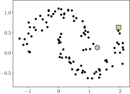
(a) Data

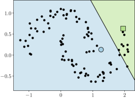
(b) Fully supervised

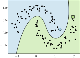
(c) Semi-supervised

Figure 1: A toy example comparing fully and semi-supervised learning. In (a) we show a data set with 2 labeled examples — the blue circle and green square — along with $98$ unlabeled data points — the black dots. In (b) we show the decision regions from training a fully supervised classification algorithm, while in (c) we show the decision regions for a semi-supervised learning algorithm, which uses the unlabeled data to inform the decision boundary.

Semi-supervised learning uses both labeled and unlabeled data. As a toy example, in Figure 1a we show the famous two-moons data set with two labeled data points; the blue circle and green square. The black points are the unlabeled data, which are not used by fully supervised learning, and we be discussed momentarily. With only two labeled data points, it is difficult to learn a general function $f$ that will correctly classify new data points. In Figure 1b we show the result of training a linear kernel support vector machine (SVM) with these two data points, which finds the linear decision boundary with maximal margin — in this case the line equidistant from the two training points. Given no other information, this may be a reasonable thing to do. However, suppose now that we also have access to the black points, which are unlabeled data points. That is, we have access to the coordinates $x_{i}\in\mathbb{R}^{2}$, but not the label $y_{i}$, which in this case is $y_{i}\in\{0,1\}$ for binary classification, and these unlabeled data points are the only data points we will want to apply our classifier to in the future. In this case, the linear SVM decision boundary is a poor choice, since it cuts through a dense region of the unlabeled data — the lower moon — where we may not expect a true decision boundary to lie. Instead, we should seek to place the decision boundary in sparse regions between clusters. In Figure 1c we show the result of using a semi-supervised learning algorithm on the same data set, which correctly separates the two moons.

There are many ways to incorporate unlabeled data into a machine learning algorithm. One common and successful approach is to utilize graph-based learning, where each node in the graph corresponds to a data point, and the edges in the graph correspond to either intrinsic relationships between data points, or record some notion of similarity between data points. Many types of data have intrinsic graph structures, like molecules in drug discovery problems, citation datasets, or networks like the internet. In other problems, like image classification, the graph structure is not intrinsic, but can be constructed as a similarity graph, in which similar data points are connected by an edge with a weight the encodes the degree of similarity. Let ${\mathcal{X}}=\{x_{1},\dots,x_{n}\}$ be a set of data points, where $x_{i}\in\mathbb{R}^{d}$. Here, we assume we have a graph with vertex set ${\mathcal{X}}$ described by a symmetric weight matrix $W=W^{T}\in\mathbb{R}^{n\times n}$ in which each entry $w_{xy}$, for $x,y\in{\mathcal{X}}$, is non-negative and encodes a notion of similarity between $x$ and $y$. A zero weight $w_{xy}=0$ indicates there is no edge between $x$ and $y$, while a positive weight $w_{xy}>0$ indicates the presence of an edge, and the large the value the stronger the edge. We let $N_{x}\subset{\mathcal{X}}$ denote the graph neighbors of the vertex $x\in{\mathcal{X}}$, which is defined by

(3.1) $$N_{x}=\{y\in{\mathcal{X}}\,:\,w_{xy}>0\}.$$

A common way to construct a graph over a data set is the geometric graph construction

(3.2) $$w_{xy}=\eta\left(\frac{|x-y|}{\varepsilon}\right),$$

where $\varepsilon>0$ is the graph bandwidth and $\eta:[0,\infty)\to[0,\infty)$ is a nonnegative function that is typically decreasing with compact support. A common choice is Gaussian weights where $\eta(t)=e^{-t^{2}}$, with a possible truncation to zero at some distance $t=\tau$. One issue with the geometric graph construction is that one has to choose a very large value for the graph bandwidth $\varepsilon>0$ to ensure the graph is connected, even in the sparsest regions of the data set, which leads to a very non-sparse weight matrix $W$ that is difficult to work with computationally. To address this, it is common to adjust the bandwidth $\varepsilon$ locally to reflect the density (or sparsity) of the data set, which results in various types of $k$-nearest neighbor graphs. One common construction is

$$w_{xy}=\eta\left(\frac{|x-y|}{\sqrt{\varepsilon_{x}\varepsilon_{y}}}\right),$$

where $\varepsilon_{i}$ is the distance from $x$ to its $k^{\rm th}$ nearest neighbor, though other choices are possible. Throughout this section, we’ll generally assume a graph with geometric weights of the form (3.2).

3.2 Laplacian regularization

Suppose now that we have a graph structure over our data set, given by a weight matrix $W=(w_{xy})\in\mathbb{R}^{n\times n}$ along with a subset of graph nodes $\Gamma\subset{\mathcal{X}}$ that are labeled, with corresponding labels $y=g(x)\in\mathbb{R}$ for $g:\Gamma\to\mathbb{R}$ a given labeling function, which we are taking to be scalar only for simplicity of discussion. The seminal approach in graph-based semi-supervised learning is Laplacian regularization, initially proposed in [123], which propagates the labels from $\Gamma$ to the rest of the graph by solving the optimization problem

(3.3) $$\min_{u:{\mathcal{X}}\to\mathbb{R}}\sum_{x,y\in{\mathcal{X}}}w_{xy}(u(x)-u(y))^{2},$$

subject to the constraint that $u(x)=g(x)$ for $x\in\Gamma$. The real-valued solution $u(x)$ is then thresholded to the nearest label to make a class prediction. The energy in (3.3) is called the graph Dirichlet energy and the minimizer $u:{\mathcal{X}}\to\mathbb{R}$ is exactly the harmonic extension of the labeled data, which satisfies the boundary value problem

(3.4) $$\left\{\begin{aligned} \mathcal{L}u(x)&=0,&&\text{if }x\in{\mathcal{X}}\setminus\Gamma\\ u(x)&=g(x),&&\text{if }x\in\Gamma,\end{aligned}\right.$$

where $\mathcal{L}$ is the graph Laplacian defined by

(3.5) $$\mathcal{L}u(x)=\sum_{y\in{\mathcal{X}}}w_{xy}(u(x)-u(y)).$$

In other words, we are seeking the smoothest function — in this case harmonic — that correctly classifies the labeled data points. In semi-supervised learning, this is often called the semi-supervised smoothness assumption [28], which stipulates that the labeling is smooth in high density regions of the data set. Since the initial development in [123], graph-based learning using Laplacian regularization, and variations thereof, has grown into a wide class of useful techniques in machine learning [2, 117, 119, 118, 121, 53, 54, 111, 114, 115, 11, 8, 12, 122, 110, 51, 68, 22, 26, 9].

Laplacian regularized learning has an important connection to random walks on graphs. Let $X_{1},X_{2},\dots$ be a random walk on the vertices ${\mathcal{X}}$ of the graph, with transition probabilities $P=D^{-1}W$, where $D=\operatorname{diag}(d_{x_{1}},\dots,d_{x_{n}})$ and $d_{x}=\sum_{y\in{\mathcal{X}}}w_{xy}$ is the degree of vertex $x$. That is, the probability $p_{xy}$ of the random walker moving from vertex $x$ to vertex $y$ is given by $p_{xy}=d_{x}^{-1}w_{xy}$. Given a function $u:{\mathcal{X}}\to\mathbb{R}$ on the vertices of the graph, we can compute

$${\mathbb{E}}[u(X_{k+1})-u(X_{k})\,|\,X_{k}=x]=\sum_{y\in{\mathcal{X}}}p_{xy}(u(y)-u(x))=-\frac{1}{d_{x}}\mathcal{L}u(x).$$

The object on the right hand side is called the random walk graph Laplacian, and we denote it by $\mathcal{L}_{rw}$; that is

$$\mathcal{L}_{rw}u(x)=\frac{1}{d_{x}}\mathcal{L}u(x).$$

The computation above thus yields

(3.6) $${\mathbb{E}}[u(X_{k+1})\,|\,X_{k}]=u(X_{k})-\mathcal{L}_{rw}u(X_{k}),$$

and thus, the random walk graph Laplacian is the generator for the random walk. In particular, if $u$ is graph harmonic, so that $\mathcal{L}u(x)=0$, then $u(X_{k})$ is a martingale. Defining the stopping time $\tau$ as the first time the random walk hits the labeled data set $\Gamma$, the optional stopping theorem yields that the solution $u$ of Laplace learning (3.4) satisfies

(3.7) $$u(x)={\mathbb{E}}[u(X_{\tau})\,|\,X_{1}=x]=\sum_{y\in\Gamma}{\mathbb{P}}(X_{\tau}=y\,|\,X_{1}=x)g(y).$$

Thus, the solution of Laplacian regularized graph-based learning (3.4) can be interpreted as a weighted average of the given labels $g(y)$, weighted by the probability of the random walk hitting $y\in\Gamma$ first, before hitting any other labeled data point. This is a reasonable thing to do for semi-supervised learning at an intuitive level as well. Indeed, if each cluster in the data set is well separated from the others, then provided the label rate is not too low, the random walk is likely to stay in the cluster it started in long enough to hit a labeled data point in that cluster, giving the correct label and propagating labels well within clusters.

At moderately low label rates, Laplacian regularization performs very well for graph-based semi-supervised learning. However, the performance can be come quite poor at extremely low label rates, which was first noted in [96] and later in [36]. When there are very few labels, the solution of the Laplace learning problem (3.4) prefers to be nearly constant over the whole graph, with sharp spikes at the labeled data points, as depicted in Figure 2a. This is the configuration that gives the least graph Dirichlet energy, since the spikes are relatively inexpensive when the number of labeled data points is small. From the random walk perspective, when there are very few labels, the random walk takes very long to hit a labeled data point, so the stopping time $\tau$ is very large, and the distribution of the random walker approaches the limiting invariant distribution on the graph, which is proportional to the degree. Thus, by (3.7) we have

(3.8) $$u(x)\approx\frac{\sum_{y\in\Gamma}d_{y}g(y)}{\sum_{y\in\Gamma}d_{y}}$$

at very low label rates. When the labels are binary $g(y)\in\{-1,1\}$, the sign of the right hand side of (3.8) is constant over the graph, and simply chooses the class whose labeled points have the largest cumulative degree, which is one way to explain the very poor performance of Laplace learning at low label rates.

Even in settings where moderate amounts of labeled data will eventually be acquired, it is often necessary to consider, at least initially, problems with very few labels where Laplace learning is not useful. One of those areas is active learning, which refers to machine learning algorithms that address the problem of choosing the best data points to label in order to obtain superior model performance with as few labels as possible [105]. Active learning methods incorporate a human-in-the-loop that can be queried to label new data points as needed, and the goal is to achieve the highest accuracy with as few labels as possible by intelligently choosing the next point to label, often in a sequential manner. Active learning procedures normally start out with extremely small labeled sets that slowly grow during the acquisition of new labeled data points, which requires graph-based semi-supervised learning algorithms that perform well both with small and moderate amounts of labeled data. A number of graph-based active learning methods have been proposed [124, 61, 80, 103, 93, 95], including recent methods inspired by the PDE-continuum limits discussed below [94], and recent applications have been found in image classification problems [41, 29, 16, 92].

Let us also mention that there is a growing body of work on deep semi-supervised learning, which includes many methods based on graph neural networks; see [116] for a survey. Many recent works have shown that one can obtain effective deep graph neural network methods for tasks including semi-supervised learning by decoupling the graph diffusion part, normally based on message passing, from the neural network [104, 48, 33, 6, 59]. Hence, improvements in graph-based semi-supervised learning can have a direct impact on deep semi-supervised learning as well.

3.3 PDE-inspired insights and algorithms

Another interpretation of the poor performance of Laplace learning at low label rates is though PDE continuum limits. To explain this, we need to place some additional assumptions on the graph construction. We assume the vertices ${\mathcal{X}}=\{x_{1},\dots,x_{n}\}$ of the graph are i.i.d. random variables distributed on a domain $\Omega\subset\mathbb{R}^{d}$ with a continuous and positive density $\rho:\Omega\to(0,\infty)$. We assume the random geometric graph construction, which uses weights (3.2) for a given bandwidth $\varepsilon>0$. This is called a random geometric graph, and in this setting, the expectation of the graph Dirichlet energy in (3.3) is

(3.9) $$n^{2}\int_{\Omega}\int_{\Omega}\eta\left(\frac{|x-y|}{\varepsilon}\right)(u(x)-u(y))^{2}\rho(x)\rho(y)\,dxdy\approx C_{\eta}n^{2}\varepsilon^{d+2}\int_{\Omega}\rho^{2}|\nabla u|^{2}\,dx,$$

provided $u:\Omega\to\mathbb{R}$ is a smooth function and $\rho$ is Lipschitz, where $C_{\eta}$ is a positive constant depending only on $\eta$. The asymptotics in (3.9) can be verified formally with Taylor expansions of $u$ and $\rho$, and can also be established rigorously in the language of Gamma convergence, as in [47]. Thus, the continuum version of Laplace learning (3.4) is the boundary value problem

(3.10) $$\left\{\begin{aligned} \operatorname{div}(\rho^{2}\nabla u)&=0,&&\text{in }\Omega\setminus\Gamma\\ u&=g,&&\text{on }\Gamma,\end{aligned}\right.$$

where $\Gamma\subset\Omega$ is purposely vaguely specified, and should encode some notion of the continuum limit of the labeled data set, and $g:\Gamma\to\mathbb{R}$ the continuum limit of the values of the labels. When $\Gamma$ does not contain the entire boundary $\partial\Omega$, we also must impose homogeneous Neumann conditions on $\partial\Omega\setminus\Gamma$.

The presence of the squared density $\rho^{2}$ as a diffusion coefficient in the PDE continuum limit illustrates how Laplace learning is able to diffuse labels quickly in high density regions where $\rho$ is large, and place decision boundaries, which correspond to sharp transitions in the label function $u$, in sparse regions where $\rho$ is small. However, the presence of the labeled set $\Gamma$ as a boundary condition is problematic, since (3.10) is well-posed only when $\Gamma$ is large enough, and regular enough. For instance, $\Gamma$ cannot be a collection of isolated points as in Figure 2a, otherwise (3.10) is ill-posed, since the capacity of a point is zero [69]. We need to be able to define the trace of a Sobolev space function in $H^{1}(\Omega)$ on $\Gamma$ in order to establish well-posedness of (3.10) [42].

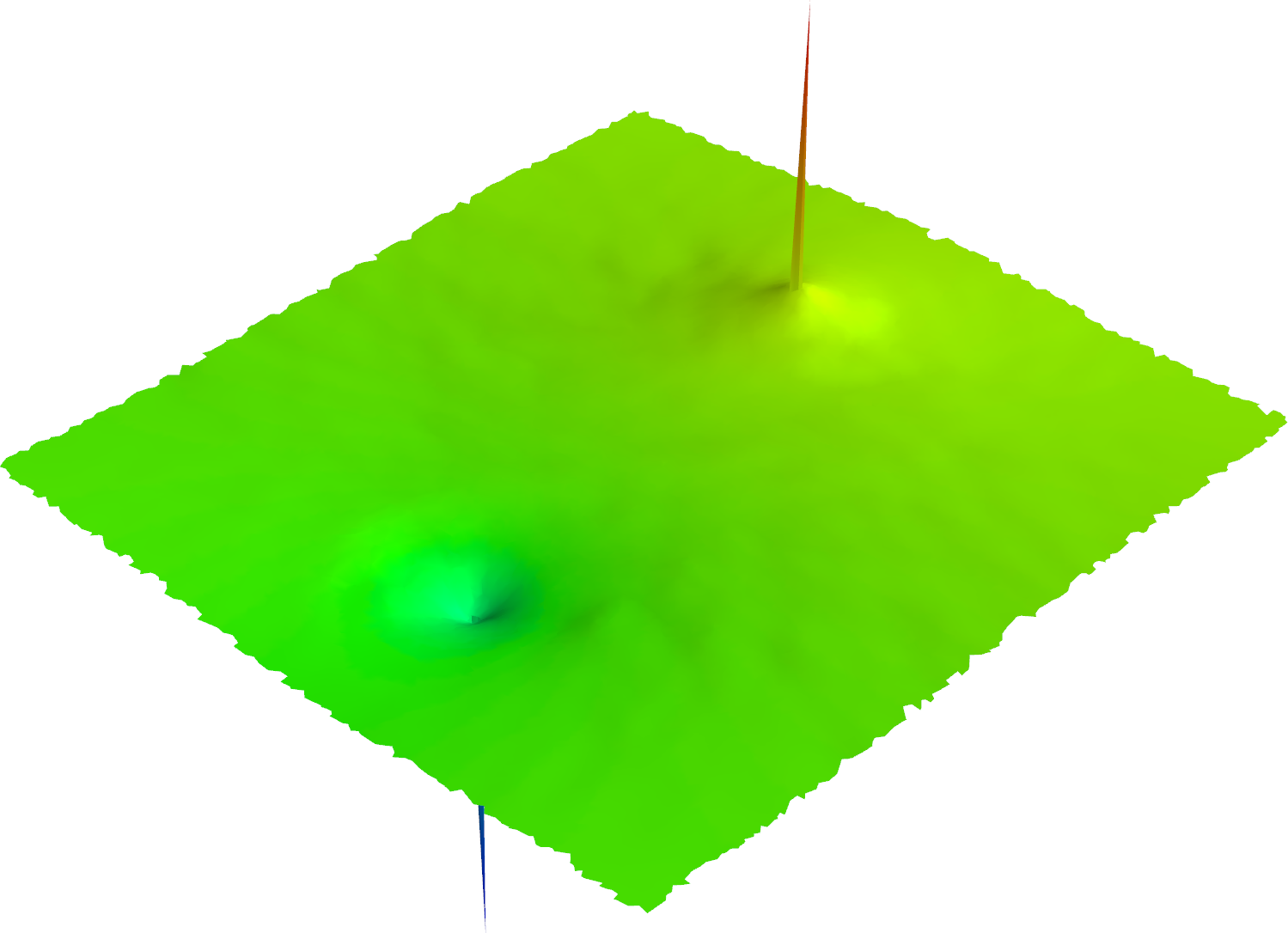
(a) Laplace [123]

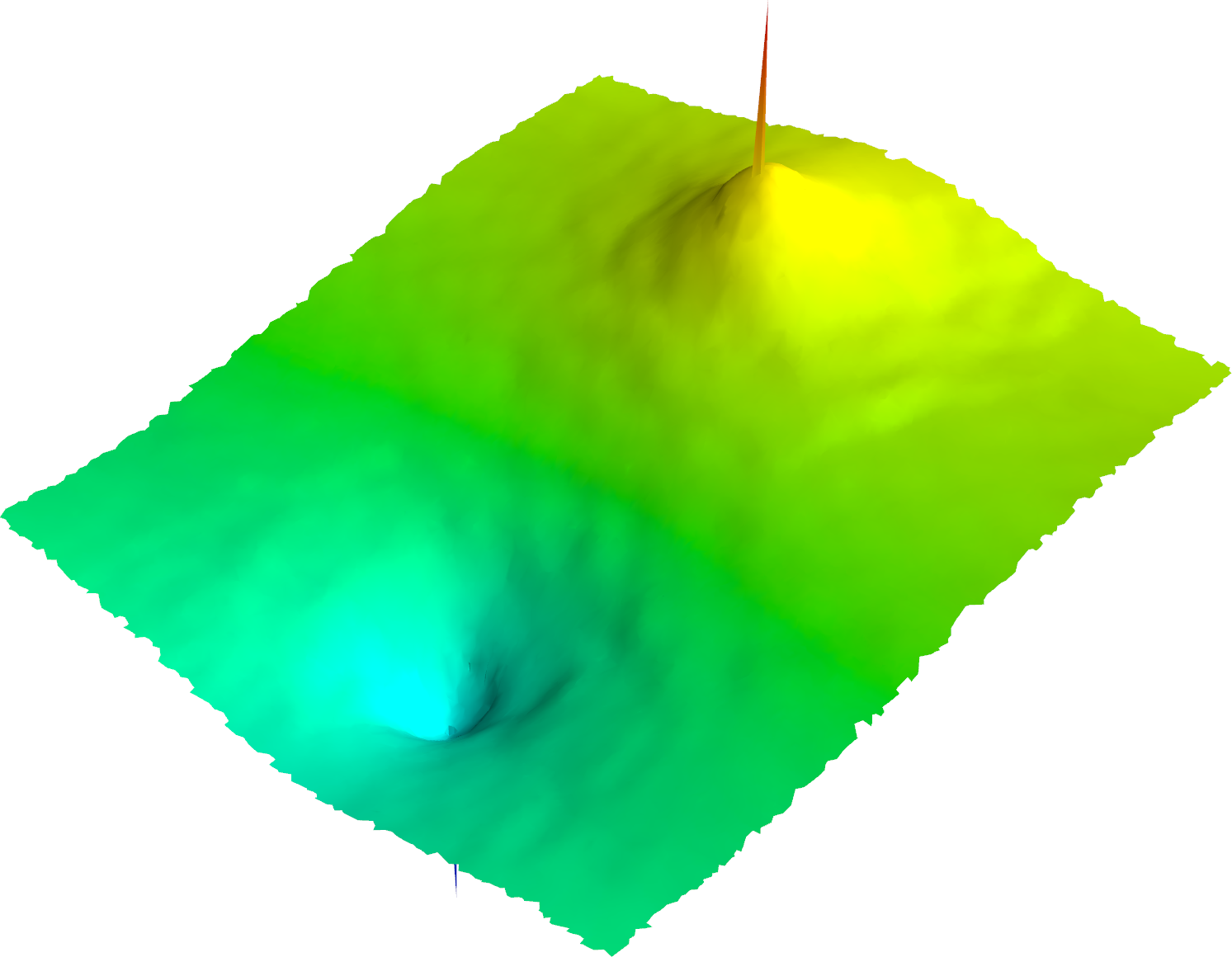
(b) $p$-Laplace, $p=2.05$ [44]

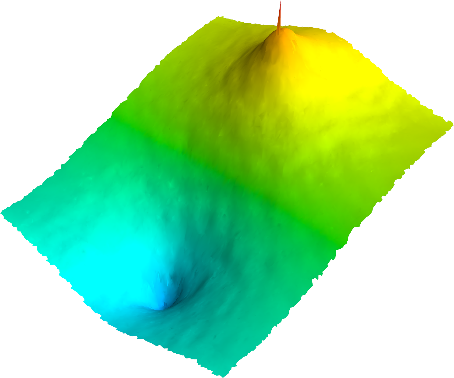
(c) $p$-Laplace, $p=2.25$ [44]

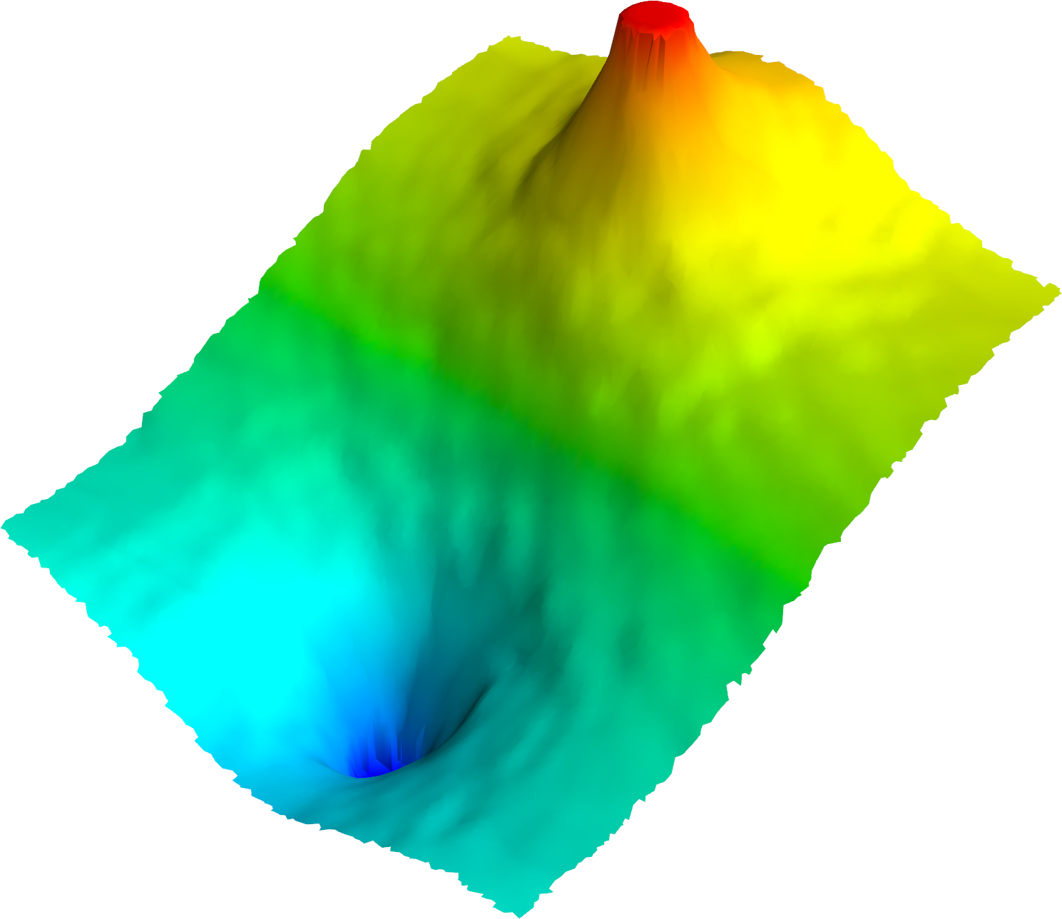
(d) WNLL [106]

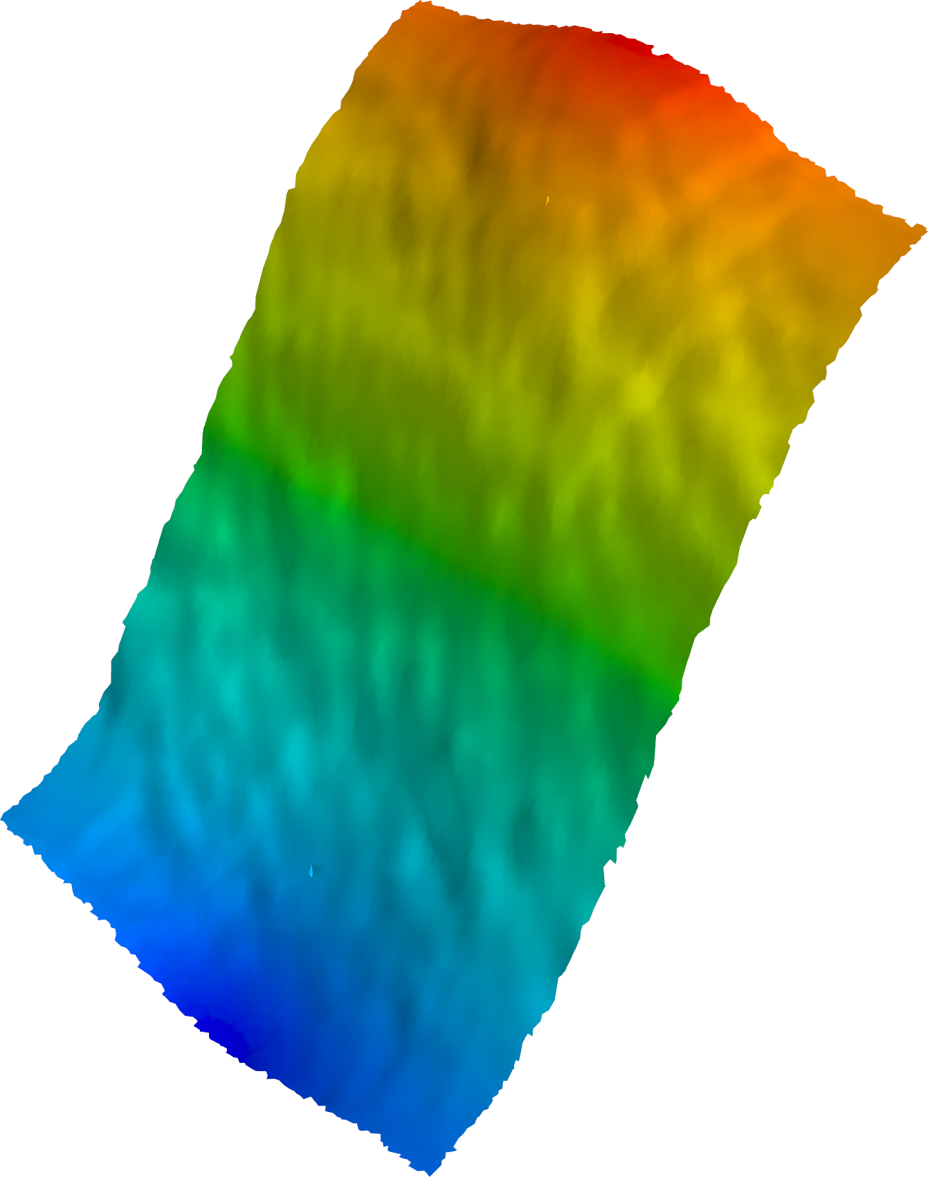
(e) High-order Laplace, $m=2$ [122]

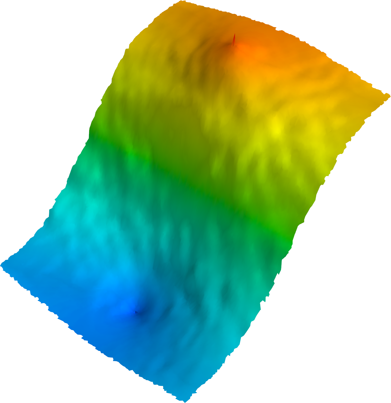
(f) PWLL [94, 21]

Figure 2: Comparison of different semi-supervised learning methods on a toy example with two labeled data points with labels $+1$ and $-1$. The graph consists of $n=20,000$ uniformly distributed random variables on the unit box $[0,1]^{2}$ with geometric Gaussian kernel weights with $\varepsilon=0.05$.

The last decade has seen a surge of interest in developing graph-based learning algorithms that are well-posed with arbitrarily small labeled data sets, by considering PDE continuum limits that are insensitive to the labeled data set. One natural idea proposed in [39] is to consider the $p$-Dirichlet energy on the graph, given by

(3.11) $$\sum_{x,y\in{\mathcal{X}}}w_{xy}|u(x)-u(y)|^{p}.$$

In fact, the $p$-Laplacian was suggested in many other works as well [1, 15, 120, 39, 37, 38, 50, 62, 40], though not in the low label rate context. By a similar argument as above, the continuum limit energy should be the weighted $p$-Dirichlet energy

$$\int_{\Omega}\rho^{2}|\nabla u|^{p}\,dx.$$

When $p>d$, we have the Sobolev embedding $W^{1,p}(\Omega)\subset C^{0,\alpha}(\Omega)$ [42], which ensures that solutions are Hölder continuous, spikes cannot form, and the continuum boundary value problem

(3.12) $$\left\{\begin{aligned} \operatorname{div}(\rho^{2}|\nabla u|^{p-2}\nabla u)&=0,&&\text{in }\Omega\setminus\Gamma\\ u&=g,&&\text{on }\Gamma,\end{aligned}\right.$$

is well-posed without any conditions on $\Gamma$. This well-posedness was established rigorously in the continuum limit in [107] when $p>d$ and the number of labeled points is finite and fixed as the number of unlabeled data points tends to infinity. In this case, the authors of [107] identified an additional restriction on the length scale $\varepsilon>0$ that arises through the nonlocal nature of the graph Laplacian. Namely, in addition to $p>d$, it is necessary that $n\varepsilon^{p}\ll 1$ to ensure that spikes do not form. Since $n\varepsilon^{d}\gg\log n$ is necessary to ensure connectivity of the graph, this condition can only be satisfied when $p>d$. The authors of [107] also proposed a modification of $p$-Laplace learning for which the condition $n\varepsilon^{p}\ll 1$ is not required, by essentially extending the labels to all nearest neighbors on the graph.

It is worthwhile to pause and note that the condition $n\varepsilon^{p}\ll 1$ comes from a simple balancing of energy between “spikey” functions and smooth functions on the graph. If we write (3.9) for the $p$-Laplacian, we see that the graph $p$-Dirichlet energy of a smooth function scales like $n^{2}\varepsilon^{p+d}$. On the other hand, the energy of a constant function with spikes at the labeled nodes is

$$\sum_{x\in\Gamma}\sum_{y\in{\mathcal{X}}}\eta\left(\frac{|x-y|}{\varepsilon}\right)|g(y)-c|^{p}\approx C|\Gamma|S^{p}n\varepsilon^{d},$$

where $C$ is a constant depending on $\eta$, $c=u(x)$ is the constant value of $u$, $S$ is the size of the spikes, and $|\Gamma|$ is the number of labeled points, all provided the label rate is sufficiently low and the labeled points are sufficiently far apart. In order to ensure that a smooth interpolating function has less energy than a spikey one, in the setting where $|\Gamma|$ is constant with $n$ and $\varepsilon$ we require

$$n^{2}\varepsilon^{p+d}\ll n\varepsilon^{d}\iff n\varepsilon^{p}\ll 1.$$

If we allow the number of labels $|\Gamma|$ to depend on $n$ and $\varepsilon$, then the condition is

$$n^{2}\varepsilon^{p+d}\ll|\Gamma|n\varepsilon^{d}\iff\beta:=\frac{1}{n}|\Gamma|\gg\varepsilon^{p}.$$

The quantity $\beta$ above is the label rate — the ratio of labeled data points to all data points — and simply energy balancing arguments show that the label rate $\beta$ should satisfy $\beta\gg\varepsilon^{p}$ to ensure convergence to a well-posed continuum problem. The case of finite labels as $n\to\infty$ corresponds to $\beta=n^{-1}$, which recovers the condition $n\varepsilon^{p}\ll 1$. In [27] it was shown that $\beta\sim\varepsilon^{2}$ for $p=2$ is the threshold for a spikey versus smooth continuum limit in a setting that allowed the labeled data set to grow as $n\to\infty$. The proofs in [27] used the random walk interpretation of the $2$-Laplacian and martingale arguments. A negative result was also established in [27] for $p>2$ showing that spikes develop when $\beta\ll\varepsilon^{p}$. However, a positive result for $p>2$ — that $\beta\gg\varepsilon^{p}$ is sufficient to prevent spikes from forming — is currently lacking, outside of the finite label regime covered in [107].

As in Section 2 we can take the limit as $p\to\infty$ of the graph $p$-Dirichlet energy. It is more illustrative to do this with the necessary conditions for minimizing the graph $p$-Dirichlet energy (3.11), which is the graph $p$-Laplace equation

(3.13) $$\sum_{y\in{\mathcal{X}}}w_{xy}|u(x)-u(y)|^{p-2}(u(x)-u(y))=0$$

for each $x\in{\mathcal{X}}\setminus\Gamma$. To take the limit as $p\to\infty$, we separate the terms in the summation above by sign, and take the $p^{\rm th}$ root to obtain

$$\left(\sum_{y\,:\,g_{xy}>0}^{n}w_{xy}(u(x)-u(y))^{p-1}\right)^{1/p}=\left(\sum_{y\,:\,g_{yx}>0}^{n}w_{xy}(u(y)-u(x))^{p-1}\right)^{1/p}.$$

where $g_{xy}=w_{xy}(u(x)-u(y))$. The terms with $g_{xy}=0$ do not contribute and can be neglected. We assume neither sum above is empty, otherwise all terms in (3.13) are zero, which is trivial. Sending $p\to\infty$ yields the equation

$$\max_{y\,:\,g_{xy}>0}(u(x)-u(y))=\max_{y\,:\,g_{yx}>0}(u(y)-u(x)).$$

The maximums above are unchanged by replacing the conditions $g_{xy}>0$ and $g_{yx}>0$ with $w_{xy}>0$, as the graph is symmetric so $w_{xy}=w_{yx}$. Making this replacement, dividing by two on both sides, and rearranging yields

(3.14) $$\mathcal{L}_{\infty}u(x):=u(x)-\frac{1}{2}\left(\max_{N_{x}}u+\min_{N_{x}}u\right)=0,$$

where $\mathcal{L}_{\infty}$ is called the graph $\infty$-Laplacian, and we recall that $N_{x}$ are the graph neigbhors of $x$ defined in (3.1). Notice the maximum and minimum above are over graph neighbors, which satisfy $w_{xy}>0$, but that the weights in the graph do not enter directly into the operator otherwise. If we were to replace $w_{xy}$ by $w_{xy}^{p}$ in (3.13), then the weights would appear in the graph $\infty$-Laplacian, which is more informative of the graph structure, and was the approach taken in [19]. We use the unweighted $\infty$-Laplacian here since it connects more directly to the tug-of-war interpretation of the graph $p$-Laplacian, discussed below in this section. It turns out, similar to the continuum $\infty$-Laplace equation, that graph $\infty$-harmonic functions also solve $L^{\infty}$-type variational problems on graphs (see, for example, [66, 79]).

The graph $\infty$-Laplacian was first used for semi-supervised learning in [79, 66], where it is called Lipschitz learning. In [20] it was shown rigorously using PDE-continuum limits that solutions of the graph $\infty$-Laplace equation converged to $\infty$-harmonic functions in the continuum, even for finite isolated labeled data points. This established well-posedness of Lipschitz learning with arbitrarily few labeled examples. Subsequent work [18, 17] established convergence rates of graph $\infty$-harmonic functions to the continuum. As in Section 2, specifically (2.6), it is natural to define a $p$-Laplacian operator on the graph that is a combination of the $2$-Laplacian and $\infty$-Laplacian. Here we use the definition

(3.15) $$\mathcal{L}_{p}=\alpha\mathcal{L}_{rw}+(1-\alpha)\mathcal{L}_{\infty},$$

where $\alpha=1/(p-1)$ and $\alpha=1$ when $p=\infty$. This type of graph $p$-Laplacian is often called the game-theoretic $p$-Laplacian due to its connection to tug-of-war games, as described in Section 2. The $p$-Laplace operator appearing earlier in (3.13), as the necessary conditions for the $p$-Dirichlet energy, is usually called the variational $p$-Laplacian, and is a different operator on the graph, even though they agree in the continuum. The game-theoretic $p$-Laplacian on graphs originally appeared in [85], and was proposed for semi-supervised learning in [19], although the latter work considered a weighted version of the $\infty$-Laplacian. In [19] it was shown that the game-theoretic $p$-Laplacian is well-posed with arbitrarily few labeled examples when $p>d$, by showing that the continuum limit was the well-posed continuum $p$-Laplace equation with $p>d$. An interesting and important detail is that the condition $n\varepsilon^{p}\ll 1$ is not required by the game-theoretic $p$-Laplacian, due to the strong regularization provided by the $\infty$-Laplacian.

As in Section 2, we can develop a tug-of-war game interpretation for the game-theoretic graph $p$-Laplacian. Any function $u$ on the graph satisfying $\mathcal{L}_{p}u=0$ also satisfies, by rearranging (3.15), the equation

(3.16) $$u(x)=\frac{\alpha}{d_{x}}\sum_{y\in{\mathcal{X}}}w_{xy}u(y)+\frac{1-\alpha}{2}\left(\max_{N_{x}}u+\min_{N_{x}}u\right),$$

which is the discrete graph version of the continuous identity (2.9), without the $O(\varepsilon)$ error term. As we did in Section 2, we can define a discrete stochastic process on the graph that produces the martingale property. We define $X_{1},X_{2},\dots$ so that, given $X_{k}$, the choice of $X_{k+1}$ is with probability $\alpha$ a random walk step from $X_{k}$, with probability $\frac{1-\alpha}{2}$ the vertex $y$ maximizing $u(y)$ over neighbors $y$ of $X_{k}$, and with probability $\frac{1-\alpha}{2}$ the corresponding minimizing vertex. For the same reasons as in Section 2, any graph $p$-harmonic function, satisfying $\mathcal{L}_{p}u(x)=0$ for all $i$, is a martingale when applied to the process $X_{k}$, in the sense that

$${\mathbb{E}}[u(X_{k+1})\,|\,X_{k}]=u(X_{k}).$$

This allows us to apply martingale techniques to study properties of the solution to the game-theoretic $p$-Laplacian on the graph. The variational graph $p$-Laplacian (3.13) does not have any such stochastic tug-of-war interpretation. To our knowledge, no existing works have used the tug-of-war interpretation of the graph $p$-Laplacian to study properties of semi-supervised $p$-Laplacian learning.

Figures 2b and 2c show the results of the game-theoretic $p$-Laplacian applied to the toy two labeled point problem, illustrating how the $p$-Laplacian corrects the spike phenomenon in Laplace learning. Note we only need $p>2$ here since $d=2$. Many other approaches have been proposed for correcting the degeneracy in Laplace learning. In [106], the authors proposed to reweight the edges of the graph that connect to labels more strongly to discourage spike formation, and to use the ordinary graph Laplacian on the reweighted graph. The method is called the Weighted Nonlocal Laplacian (WNLL). Figure 2d shows an example of the WNLL on the two-point problem, where we can see that the method essentially just extends the labels to nearest neighbors on the graph. However, it was shown in [26] that the WNLL method remains ill-posed at arbitrarily low label rates. In [26], the authors proposed the properly weighted graph Laplacian, which reweights the graph in a non-local way that is singular near the labeled data, so that the continuum limit is well-posed with arbitrarily few labels. In [122], it was proposed to use a higher order Laplace equation of the form $\mathcal{L}^{m}u=0$ for problems with very few labels. The idea here is that in the continuum, the variational formulation of the equation would involve $u\in H^{m}(\Omega)$, and when $\frac{m}{2}>d$, the Sobolev embedding $H^{m}\subset C^{0,\alpha}(\Omega)$ ensures that spikes do not form and the continuum limit is well-posed. Figure 2e shows the two-point problem with higher order Laplacian regularization. The well-posedness of higher order Laplace learning with finite labeled data in the continuum limit was only very recently addressed in [112]. Finally, there is recent work on using Poisson equations on graphs for semi-supervised learning in [22, 21, 94], some of which connects to the earlier work on the properly weighted Laplacian [26]. In particular, the Poisson Weighted Laplace Learning (PWLL) method from [94, 21] involves reweighting the graph using the solution of a graph Poisson equation, whose singularities are sufficient to invoke the results in [26], though the theory for these methods is currently still under development. Figure 2f shows the behavior of PWLL on the two point problem. The volume constrained MBO method based on auction dynamics developed in [60] has also proven to be effective at low label rates, though we are not aware of any theory to explain this. Other methods at low label rates include Hamilton-Jacobi equations on graphs [23] and the centered kernel method [81, 83, 82]. We also mention here the work on MBO methods for graph-based semi-supervised learning [90, 58, 45, 14, 88, 89] which consider approximations of the $p=1$ Laplacian termed MBO schemes for their connection to the Merriman-Bence-Osher threshold dynamics methods for approximating mean curvature motion [91].

3.4 Consistency versus well-posedness

(a) Data

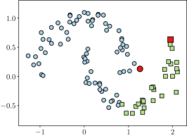
(b) Laplace [123] (77%)

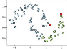
(c) $p$-Laplace [44] (79%)

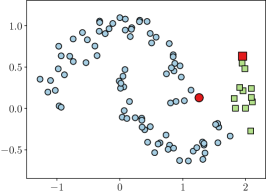
(d) WNLL [106] (61%)

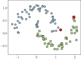
(e) High-order Laplace [122] (94%)

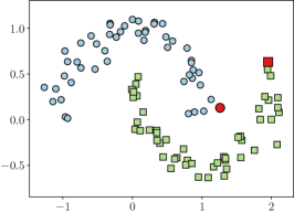
(f) Poisson [22] (100%)

Figure 3: Classification results using different graph-based semi-supervised learning algorithms on the two-moons data set. The red points are the only labeled data points. The $p$-Laplace method used $p=3$, while high order Laplace learning used order $m=4$, both of which gave the best results over a reasonable search.

Much of the work described above is aimed at establishing continuum PDE or variational descriptions of graph-based machine learning algorithms, which can, for example, prove that a method like $p$-Laplace learning provides a well-posed method for propagating labels on graphs that does not develop spikes or other degeneracies. Many other works have also considered the continuum limit of the graph Laplacian, its spectrum, and regularity properties [24, 35, 46, 55, 56, 25]. However, this abundance of work fails to address the problem of whether the machine learning methods work well or not; that is, they say little or nothing about whether the predicted label is correct! This is the question of consistency, which is more important and difficult, and thus less often studied.

As an example, in Figure 3 we show the results of graph-based semi-supervised learning applied to the same two-moons example as in Figure 1. The $p$-Laplace and higher order Laplace methods are the only methods with rigorous well-posedness results with very few labels, and Poisson learning is expected to enjoy such results, which is the subject of a forthcoming paper by the first author. Laplace learning and WNLL are ill-posed in the low-label regime. The best performing method is Poisson learning [22], followed closely by high-order Laplace, which illustrates that well-posedness does not always go hand in hand with good consistency properties, or at least that the relation between consistency and having a well-posedness continuum limit is not clear or well-understood.

To address the consistency problem, one has to make an assumption on the underlying cluster structure of the graph, or the labeling function. Then the goal is to prove that the machine learning algorithm can identify the clusters or correct labels, under reasonable assumptions on the model and parameters. This kind of consistency analysis was carried out in the context of spectral clustering in [57], in which the probability density $\rho$ was assumed to be highly concentrated on disjoint clusters. Spectral clustering uses the eigenvectors of the graph Laplacian for clustering [109] and are closely related to spectral methods in data science [34, 10, 32]. Another related work is [108], which assumes a well-separated mixture model for the data and shows that the spectral embedding reflects the clusters in the data [108]. Aside from these examples, there is a lack of consistency results for many graph-based semi-supervised learning methods, which should be viewed as an opportunity to utilize powerful PDE-continuum limit tools to establish important and interesting results about machine learning algorithms. We begin such a study in this paper.

4 Consistency results for the $p$-Laplacian

We present here a general framework for proving consistency results for graph-based semi-supervised learning with the game-theoretic $p$-Laplacian. The framework is based on the stochastic tug-of-war interpretation of the $p$-Laplacian on a graph, that was introduced in Section 3. We illustrate how to use the framework to prove some preliminary consistency results on geometric graphs and stochastic block model graphs, and then highlight some open research questions for future work.

As in Section 3 let ${\mathcal{X}}=\{x_{1},\dots,x_{n}\}$ denote our data points, which are the vertices of the graph, and let $W=(w_{xy})_{x,y\in{\mathcal{X}}}$ be a symmetric (i.e., $w_{xy}=w_{yx}$) weight matrix which encodes the graph structure. We assume the graph is connected. We let $d_{x}=\sum_{y\in{\mathcal{X}}}w_{xy}$ be the degree of vertex $x\in{\mathcal{X}}$, and we recall that $N_{x}\subset{\mathcal{X}}$ denotes the graph neighbors of $x$, as defined in (3.1). Let $\ell^{2}({\mathcal{X}})$ denote the space of functions $u:{\mathcal{X}}\to\mathbb{R}$, and define the game-theoretic $p$-Laplacian on the graph $G$ is the operator $\mathcal{L}_{p}:\ell^{2}({\mathcal{X}})\to\ell^{2}({\mathcal{X}})$ defined in (3.15) in Section 3, where $\alpha=1/(p-1)$ and $p\geq 2$. Let us denote by $\Gamma\subset{\mathcal{X}}$ the labeled data set and $g:\Gamma\to\mathbb{R}$ the labels. The game-theoretic $p$-Laplacian regularized semi-supervised learning problem is given by the boundary value problem

(4.1) $$\left\{\begin{aligned} \mathcal{L}_{p}u&=0,&&\text{in }{\mathcal{X}}\setminus\Gamma\\ u&=g,&&\text{on }\Gamma.\end{aligned}\right.$$

Since the graph is connected, the $p$-Laplace equation (4.1) can be shown to have a unique solution via the Perron method [19].

In this section we address the question of consistency of $p$-Laplacian regularization. That is, supposing that $g$ is the restriction to $\Gamma$ of a label function on the whole graph $g:{\mathcal{X}}\to\mathbb{R}$ that is in some sense smooth with respect to the geometry of the graph, we aim to give conditions under which the solution $u$ of (4.1) is close to $g$ at the unlabeled vertices ${\mathcal{X}}\setminus\Gamma$. In other words, consistency asks the question: under what conditions on the underlying label function $g$, the graph structure $W$, and the label set $\Gamma$ does the solution of $p$-Laplacian regularization make the correct label predictions?

In consistency of graph-based learning, it is essential that the underlying label function $g$ is in some way regular or smooth with respect to the graph structure. In other words, there should be some degree of correlation between the labels of vertices and their nearby neighbors in the graph topology. Otherwise graph-based learning is not useful and would not be expected to yield better results than fully supervised learning that ignores the graph structure. In this section, we present results for two different types of graph structures. In Section 4.2 we present results for geometric graphs, where the vertices are sampled from a Euclidean domain and nearby points are connected by edges. In this case we assume that $g$ has some degree of regularity with respect to the underlying Euclidean geometry. In Section 4.3 we present results for classification on stochastic block model graphs, where there is no underlying geometry. In this case the label function is concentrated on the blocks, and only changes between blocks where there are relatively few edges.

4.1 Results on general graphs

Before presenting our main results in Section 4.2 and Section 4.3, we present our general stochastic tug-of-war framework on general graphs in Section 4.1.1, which amounts to selecting sub-optimal strategies in the tug-of-war game to produce tractable upper and lower bounds on the solution $u$ of the $p$-Laplace equation (4.1). It is interesting to remark that we do not explicitly use the symmetry assumption $w_{xy}=w_{yx}$ in our results, and our results hold with minor modifications to the quantities involved for directed (i.e., nonsymmetric) graphs.

4.1.1 The tug-of-war lemma

In this section we present our main tug-of-war result (Lemma 4.3), which uses the stochastic tug-of-war game and martingale techniques to bound the difference $u(x)-g(x)$, where $u$ solves (4.1). These techniques are later applied to geometric graphs in Section 4.2, and to stochastic block model (SBM) graphs in Section 4.3. Throughout the rest of the paper, we make the simplifying assumption that every vertex $x\in{\mathcal{X}}$ has a neighbor $y\in N_{x}$ with $y\in\Gamma$, meaning:

• We assume that for every $x\in{\mathcal{X}}$

  $$\Gamma\cap N_{x}\neq\varnothing.$$

In Sections 4.2 and 4.3 we will give conditions under which (A1) holds for geometric and SBM graphs. The tug-of-war game for the $p$-Laplacian is based on the following dynamic programming principle associated with the $p$-Laplacian, which was discussed and established in Section 3.

Proposition 4.1 (Dynamic Programming Principle).

If $u\in\ell^{2}({\mathcal{X}})$ and $x\in{\mathcal{X}}$ such that $\mathcal{L}_{p}u(x)=0$ then

(4.2) $$u(x)=\frac{\alpha}{d_{x}}\sum_{y\in{\mathcal{X}}}w_{xy}u(y)+\frac{1-\alpha}{2}\left(\min_{N_{x}}u+\max_{N_{x}}u\right),$$

where we recall that $\alpha=1/(p-1)$ and $p\geq 2$.

We call equation (4.2) a dynamic programming principle (DPP), because it expresses $u$ at a point via $u$ at nearby points, and is closely related to the DPPs that appear in optimal control problems (see, e.g., [7]). In fact, the DPP arises from the stochastic two player tug-of-war game described in Section 3. The game is played between two players Paul and Carol. The game ends when the token of the game arrives at a point $x\in\Gamma$, and Paul pays Carol $g(x)$. Thus, Paul wants the game to end where $g$ is smallest, while Carol wants the opposite. At each step of the game, with probability $\alpha$ the token moves from its current position $x$ to a neighbor $y\in N_{x}$ via a single step of a random walk on the graph (i.e., the next position is chosen randomly according to the distribution ${\mathbb{P}}(y)=w_{xy}/d_{x}$). With probability $(1-\alpha)/2$ Paul chooses the next position of the token, and with probability $(1-\alpha)/2$ Carol chooses the next position. We will use this interpretation in the proofs of our main results, without explicitly writing down the game or the appropriate spaces of strategies.

In order to use the tug-of-war game, we define a stochastic process that corresponds to a sub-optimal strategy for Paul. We recall that $\alpha=1/(p-1)$ and pick any $p\geq 2$. Let $u\in\ell^{2}({\mathcal{X}})$ and $x\in{\mathcal{X}}$, and consider the following stochastic process defined on ${\mathcal{X}}$ associated with $u$ and an initial point $x\in{\mathcal{X}}$. We define the sequence of random variables $X_{0},X_{1},X_{2}$ as follows. We first set $X_{0}=x$. Then, conditioned on $X_{i}$, we choose $X_{i+1}$ as follows: first, if $X_{i}\in\Gamma$, then we set $X_{i+1}=X_{i}$, so the process gets stuck when it hits $\Gamma$. If $X_{i}\not\in\Gamma$, then we choose $X_{i+1}$ by the following:

1. With probability $\alpha$ we take an independent random walk step, that is

   $${\mathbb{P}}(X_{i+1}=y\,|\,X_{i}=x)=\frac{w_{xy}}{d_{X}}.$$

2. With probability $\tfrac{1}{2}(1-\alpha)$ we choose $\displaystyle X_{i+1}\in\operatorname*{argmax}_{y\in N_{X_{i}}}u$.

3. With probability $\tfrac{1}{2}(1-\alpha)$ we choose $\displaystyle X_{i+1}\in\operatorname*{argmin}_{y\in N_{X_{i}}\cap\Gamma}g$.

All the probabilistic ingredients are chosen independently. When there are multiple choices for $X_{i+1}$ in steps 2 and 3, the particular choice is irrelevant to the analysis, and any concrete choice will do (e.g., say, choose the vertex $x_{i}$ with the smallest index). The stochastic process $X_{0},X_{1},X_{2},\dots,$ defined above can be interpreted as a realization of the two-player game where Carol plays optimally and our choice of strategy for Paul is to move to $\Gamma$ as soon as possible. The assumption (A1) assures that there will always be a choice for Paul to make in step 3.

We now establish the sub-martingale property corresponding to our stochastic process.

Lemma 4.2.

Assume (A1) and let $u$ be the solution to (4.1). Then the random variables $Z_{i}=u(X_{i})$ form a sub-martingale with respect to $X_{i}$, that is ${\mathbb{E}}[Z_{i+1}\,|\,X_{i}]\geq Z_{i}$.

Proof.

Conditioned on $X_{i}\in\Gamma$ we have ${\mathbb{E}}[u(X_{i+1})\,|\,X_{i}]=u(X_{i})$, since $X_{i+1}=X_{i}$. Conditioned on $X_{i}\not\in\Gamma$ we further condition on steps 1–3 in the definition of $X_{i+1}$ to obtain

(4.3) $${\mathbb{E}}[u(X_{i+1})\,|\,X_{i}]=\frac{\alpha}{d_{X_{i}}}\sum_{y\in{\mathcal{X}}}w_{X_{i},y}u(y)+\frac{1-\alpha}{2}\left(\max_{N_{X_{i}}}u+\min_{N_{X_{i}}\cap\Gamma}g(y)\right).$$

Using Proposition 4.1 and $u=g$ on $\Gamma$ we have

$${\mathbb{E}}[u(X_{i+1})\,|\,X_{i}]\geq\frac{\alpha}{d_{X_{i}}}\sum_{y\in{\mathcal{X}}}w_{X_{i},y}u(y)+\frac{1-\alpha}{2}\left(\max_{N_{X_{i}}}u+\min_{y\in N_{X_{i}}}u\right)=u(X_{i}),$$

which completes the proof. ∎

The sub-martingale property allows us to bound the difference $u(x)-g(x)$ in terms of an average of the difference over the boundary. This is our main tug-of-war lemma.

Lemma 4.3.

Assume (A1) and let $u$ be the solution to (4.1). Define the stopping time

(4.4) $$\tau=\inf\{i\geq 0\,:\,X_{i}\in\Gamma\}.$$

Then for any $x\in{\mathcal{X}}$ it holds that

(4.5) $$u(x)-g(x)\leq{\mathbb{E}}[g(X_{\tau})-g(x)\,|\,X_{0}=x].\$$

Proof.

By Lemma 4.2, $Z_{i}=u(X_{i})$ is a sub-martingale, and so by Doob’s Optional Stopping Theorem for sub-martingales, see e.g. [113], we have

(4.6) $$u(x)={\mathbb{E}}[Z_{0}\,|\,X_{0}=x]\leq{\mathbb{E}}[Z_{\tau}\,|\,X_{0}=x]={\mathbb{E}}[u(X_{\tau})\,|\,X_{0}=x]={\mathbb{E}}[g(X_{\tau})\,|\,X_{0}=x],$$

since $X_{\tau}\in\Gamma$. Subtracting $g(x)$ from both sides of (4.6) completes the proof. ∎

4.1.2 General consistency results

Here, we use the martingle lemma, Lemma 4.3, to establish some general consistency results. For $g:{\mathcal{X}}\to\mathbb{R}$, we denote by $\nabla g(x,y)$ the graph gradient of $g$ defined by $\nabla g(x,y)=g(x)-g(y)$ and we set

$$\|g\|_{\infty}=\max_{x\in{\mathcal{X}}}|g(x)|,$$

and

$$\|\nabla g\|_{\infty}=\max_{x,y\in X}\Big{\{}\Big{|}(g(x)-g(y))\mathbbm{1}_{w_{xy}>0}\Big{|}\Big{\}}.$$

This is to say, the norm $\|\nabla g\|_{\infty}$ is the maximal absolute difference of $g$ across all edges in the graph.

Remark 4.4.

The quantity $\|\nabla g\|_{\infty}$ is small when the graph is embedded in Euclidean space, every edge is between nearby nodes, and $g$ is Lipschitz continuous. For example, $\varepsilon$-graphs satisfy this criterion. Hence, there $\|\nabla g\|_{\infty}\leq\varepsilon\operatorname{Lip}(g)$, because every edge is between vertices at most $\varepsilon$ apart.

Define the smallest weighted ratio of labeled neighbours to neighbours to be

(4.7) $$\delta:=\min_{x\in X}\frac{\Sigma_{y\in{\mathcal{X}}}w_{xy}\mathbbm{1}_{y\in\Gamma}}{\Sigma_{z\in{\mathcal{X}}}w_{xz}}.$$

Note that if (A1) holds, then $\delta>0$.

The following theorem gives our first consistency result on general graphs.

Theorem 4.5.

Assume (A1) holds. Then, for any $x\in{\mathcal{X}},$

(4.8) $$|u(x)-g(x)|\leq\left(\frac{2\log(\|g\|_{\infty}\|\nabla g\|_{\infty}^{-1})}{1-\alpha+2\alpha\delta}+2\right)\|\nabla g\|_{\infty}.$$

Proof.

Throughout the proof let us write $\zeta=\|\nabla g\|_{\infty}$ for simplicity. Define the stopping time $\tau$ as in (4.4). By Lemma 4.3, we have that

$$u(x)-g(x)\leq{\mathbb{E}}[g(X_{\tau})-g(x)\,|\,X_{0}=x].$$

Let us estimate the right hand side above by fixing some $k$ (which we will choose shortly) and conditioning on $\tau>k$ or $\tau\leq k$. For simplicity of notation we will drop the conditioning $X_{0}=x$ below. Then we have

(4.9) $$u(x)-g(x)={\mathbb{E}}[g(X_{\tau})-g(x)\,|\,\tau\leq k]{\mathbb{P}}(\tau\leq k)+{\mathbb{E}}[g(X_{\tau})-g(x)\,|\,\tau>k]{\mathbb{P}}(\tau>k).$$

First, we estimate the probability ${\mathbb{P}}(\tau>k).$ Since each vertex has a labeled neighbour (by Assumption (A1)), each step has probability at least $\tfrac{1}{2}(1-\alpha)+\alpha\delta$ of hitting $\Gamma$ and exiting, so a general estimate is

(4.10) $${\mathbb{P}}(\tau>k)\leq\left[1-\tfrac{1}{2}(1-\alpha)-\alpha\delta\right]^{k}\leq e^{-\frac{k}{2}(1-\alpha)-\alpha\delta k}.$$

For any $k$, we can use a telescoping series to obtain

$$g(X_{k})-g(x)=\sum_{j=0}^{k-1}(g(X_{j+1})-g(X_{j}))\leq\sum_{j=0}^{k-1}\|\nabla g\|_{\infty}=k\zeta.$$

It follows that

(4.11) $${\mathbb{E}}[g(X_{\tau})-g(x)\,|\,\tau\leq k]\leq k\zeta.$$

Substituting (4.10) and (4.11) in (4.9), we have that

(4.12) $$u(x)-g(x) \leq k\zeta{\mathbb{P}}(\tau\leq k)+{\mathbb{E}}[g(X_{\tau})-g(x)\,|\,\tau>k]e^{-\frac{k}{2}(1-\alpha)-\alpha\delta k}$$

$$\leq k\zeta+2\|g\|_{\infty}e^{-\frac{k}{2}(1-\alpha)-\alpha\delta k}.$$

We want to balance the two terms in the right hand side of (4.12), so we choose $k$ so that

$$\zeta=\|g\|_{\infty}e^{-\frac{(1-\alpha)k}{2}-\alpha\delta k},$$

or equivalently

$$k=\frac{2\log(\|g\|_{\infty}/\zeta)}{1-\alpha+2\alpha\delta}.$$

Therefore we have

(4.13) $$u(x)-g(x) \leq\zeta(k+2)=\left(\frac{2\log(\|g\|_{\infty}/\zeta)}{1-\alpha+2\alpha\delta}+2\right)\zeta.$$

To estimate $g-u$, we use a similar argument, where we replace $u$ by $-u$ and $g$ by $-g$. This concludes the proof. ∎

It turns out we can use the same argument to establish a Lipschitz estimate on the solution $u$ of the $p$-Laplace equation.

Theorem 4.6.

Assume (A1) holds, and let $x$ and $y$ be two neighbors on the graph. Then,

$$|u(x)-u(y)|\leq\left(\frac{4\log(\|g\|_{\infty}\|\nabla g\|_{\infty}^{-1})}{1-\alpha+2\alpha\delta}+5\right)\|\nabla g\|_{\infty}.$$

Proof.

We apply the triangle inequality

$$|u(x)-u(y)|\leq|u(x)-g(x)|+|u(y)-g(y)|+|g(x)-g(y)|$$

and use the bound in Theorem 4.5 twice, noting that $g(x)-g(y)=\nabla g(x,y)$. ∎

Remark 4.7.

Observe that if $g$ varies slowly, then $\zeta$ is small, thus the difference $|u(x)-u(y)|$ is small. Therefore, smoothness of $g$ over the graph implies smoothness of $u$.

4.1.3 Vertex classification consistency results

We now turn to vertex classification results, where the label function $g:{\mathcal{X}}\to\mathbb{R}$ takes constant values, and hence it will have sharp transitions across edges in the graph. Thus, $\|\nabla g\|_{\infty}$ may not be small, and so Theorems 4.5 and 4.6 are not applicable. We will focus on binary classification, where every point $x\in{\mathcal{X}}$ has a label zero or a label one, so $g:{\mathcal{X}}\to\{0,1\}$. To use the $p$-Laplace equation (4.1), we solve the equation with the binary values for the boundary condition $g:\Gamma\to\{0,1\}$, and threshold the solution $u(x)$ at $\frac{1}{2}$ to obtain a binary label prediction for each vertex $x\in{\mathcal{X}}\setminus\Gamma$. Thus, we make the following definition.

Definition 4.8.

Given $g:{\mathcal{X}}\to\{0,1\}$, a point $x\in{\mathcal{X}}$ is classified correctly if $g(x)=\mathds{1}_{u(x)\geq\frac{1}{2}}$, where $u$ is the solution to (4.1).

In this section, we focus on identifying which points in the graph are classified correctly. This requires a few definitions.

Definition 4.9.

A path on the graph is a sequence of edges which joins a sequence of vertices. The length of a path is the number of edges the path consists of.

Definition 4.10.

The distance $\operatorname{dist}(x,y)$ between two vertices $x,y\in{\mathcal{X}}$ is the length of the shortest path connecting the vertices. The distance between a vertex $x$ and a set of vertices $A\subset{\mathcal{X}}$, denoted $\operatorname{dist}(x,A)$, is the smallest distance between $x$ and any of the vertices $y\in A$.

For $i=0,1$ we define

(4.14) $${\mathcal{X}}_{i}=\{x\in{\mathcal{X}}:g(x)=i\}$$

and note that ${\mathcal{X}}={\mathcal{X}}_{0}\cup{\mathcal{X}}_{1}$. For any integer $m\geq 0$ and $i=0,1$, we define

$$A_{m}^{i}=\{x\in{\mathcal{X}}_{i}:\operatorname{dist}(x,{\mathcal{X}}_{1-i})\leq m\},$$

and note that $A_{m}=A_{m}^{0}\cup A_{m}^{1}$. That is to say, $A_{m}^{0}$ is the set of points from class $0$ that are at most $m$ steps away from the set of class $1$ points, and vice-versa for $A_{m}^{1}$. This means that when $m$ is small, the set $A_{m}$ contains points that are sufficiently close to the boundary between the two classes that we may expect data points in $A_{m}$ to be misclassified.

Observe that for any $x\in{\mathcal{X}}$ there is a positive probability of at least $\tfrac{1-\alpha}{2}+\alpha\delta=\tfrac{p-2+2\delta}{2(p-1)}$ of hitting the boundary $\Gamma.$ Even when $p=2,$ this probability is positive, since it is exactly $\delta>0$. We use this to establish the classification bound below, which shows that whenever a vertex $x$ is sufficiently far, in terms of graph distance, away from the true decision boundary, it will be classified correctly.

Theorem 4.11.

Assume (A1). Let $k$ be the smallest integer strictly larger than

(4.15) $$\frac{2\log(2)}{1-\alpha+2\alpha\delta}=\frac{2(p-1)\log(2)}{p-2+2\delta}.$$

Then every $x\not\in A_{k}$ is classified correctly.

Proof.

Let $x\in{\mathcal{X}}\setminus A_{k}$ and assume $X_{0}=x$. Define the stopping time $\tau$ as in (4.4). For any point $x\in{\mathcal{X}}$ we have that

(4.16) $$u(x)-g(x)\leq{\mathbb{E}}[g(X_{\tau})-g(x)\,|\,\tau\leq k]{\mathbb{P}}(\tau\leq k)+{\mathbb{E}}[g(X_{\tau})-g(x)\,|\,\tau>k]{\mathbb{P}}(\tau>k).$$

We want to classify $x$ correctly whether it belongs to ${\mathcal{X}}_{0}$ or ${\mathcal{X}}_{1}.$ Recall that the labels of vertices in ${\mathcal{X}}_{0}$ are zeros and in ${\mathcal{X}}_{1}$ are ones.

Since $x\notin A_{k}$, the labels of vertices reached by the stopping time $\tau\leq{k}$ can only be labels from the same-class, so $g(X_{\tau})=g(x).$ Thus, when $\tau\leq{k}$ the first term on the right hand side of (4.16) is zero. Then, using that $g$ is between zero and one, and that equation (4.10) holds, we obtain

(4.17) $$u(x)-g(x)\leq{\mathbb{E}}[g(X_{\tau})-g(x)\,|\,\tau>{k}]{\mathbb{P}}(\tau>{k})\leq{\mathbb{P}}(\tau>{k})\leq e^{-\frac{{k}}{2}(1-\alpha)-\alpha\delta{k}}$$

The analogous estimate on $g-u$ is similarly obtained, and so we have

$$|u(x)-g(x)|\leq e^{-\frac{{k}}{2}(1-\alpha)-\alpha\delta{k}}.$$

For correct classification of $x$, we need precisely $|u(x)-g(x)|<\frac{1}{2},$ which is equivalent to

$$e^{-\frac{{k}}{2}(1-\alpha)-\alpha\delta{k}}<\frac{1}{2},$$

and is satisfied by the choice of $k$ in (4.15)

∎

4.2 Geometric graphs

In this section we specialize our results to geometric graphs, which include the very commonly used random geometric $\varepsilon$-graphs and $k$-nearest neighbor ($k$-NN) graphs. The purpose of this section is to provide conditions under which $\varepsilon$-graphs and $k$-NN graphs, along with other graphs with geometric $\varepsilon$-scaling, fulfill the general assumption (A1) in Section 4.1.1, so that we can apply the theory developed in Section 4.1.1 to these graphs.

4.2.1 Main assumptions

In order to construct $\varepsilon$-graphs and $k$-NN graphs and construct the labeled data set $\Gamma$, we need the following assumptions. Note that assumptions (A2),(A3),(A4) also appear in [27].

• Let $d\geq 2$ and let $\Omega\subset\mathbb{R}^{d}$ be an open, bounded, and connected domain with a Lipschitz boundary. Let $x_{1},x_{2},\dots,x_{n}$ be i.i.d. with continuous density $\rho$ satisfying

  $$0<\rho_{\min}:=\inf_{x\in\Omega}\rho(x)\leq\sup_{x\in\Omega}p(x)=:\rho_{\max}<\infty.$$

  We define ${\mathcal{X}}=\{x_{1},x_{2},\dots,x_{n}\}.$

• We construct $\Gamma$ in the following way. Let $g\in\operatorname{Lip}({\overline{\Omega}})$, where $\Omega$ is defined as in (A2). Let $\beta\in(0,1)$. For each $x\in{\mathcal{X}}$, define an independent random variable $z(x)\sim Bernoulli(\beta)$ and assign $x\in\Gamma$ whenever $z(x)=1$. Each training data point $x\in\Gamma$ is assigned a label $g(x)$.

• We define an interaction potential $\eta:[0,\infty)\to[0,\infty)$. The interaction potential $\eta(\cdot)$ has support on the interval $[0,1]$, it is non-increasing, and $\eta$ restricted to $[0,1]$ is Lipschitz continuous. For $t\geq 1$ we extend $\eta$ so that $\eta(t)=0.$ Moreover, $\eta(\tfrac{1}{2})>0$ and $\eta$ integrates to $1:$

  $$\int_{\mathbb{R}^{d}}\eta(|x|)dx=1.$$

  We define $\eta_{\varepsilon}(t)=\frac{1}{\varepsilon^{d}}\eta(t/\varepsilon).$

• (Geometric graphs of length $\varepsilon$) There exist positive constants $c_{1},c_{2},\varepsilon_{1},\varepsilon_{2}$ such that for every $x,y\in{\mathcal{X}}$ we have that

  $$c_{1}\varepsilon_{1}^{-d}\mathbbm{1}_{|x-y|<\varepsilon_{1}}\leq w_{xy}\leq c_{2}\varepsilon_{2}^{-d}\mathbbm{1}_{|x-y|<\varepsilon_{2}}.$$

We note that assumptions (A2) and (A4) are used in the $\varepsilon-$graph construction (see Section 4.2.2). In Lemma 4.13 we prove that assumption (A5) holds for $\varepsilon$-graphs. Assumption (A3) has to do with how the labeled data points are chosen, and we note that the parameter $\beta\in(0,1)$ is the label rate.

Assumption (A2) is satisfied for $k$-NN-graphs by construction. In Lemma 4.17 we prove that assumption (A5) holds with high probability for $k$-NN graphs. Applying (A5), we prove (A1) holds with high probability, which means that Theorems 4.5 and 4.6 hold. For $x\in{\mathcal{X}}$ we define $d_{n}(x)$ and $p_{n}(x)$ as follows:

(4.18) $$d_{n}(x)=\Sigma_{y\in{\mathcal{X}}}w_{xy},$$

(4.19) $$p_{n}(x)=\Sigma_{y\in{\mathcal{X}}}w_{xy}\mathbbm{1}_{y\in\Gamma}.$$

Then, as before, we define

(4.20) $$\delta=\min_{x\in{\mathcal{X}}}\frac{p_{n}(x)}{d_{n}(x)}=\min_{x\in{\mathcal{X}}}\frac{\Sigma_{y\in{\mathcal{X}}}w_{xy}\mathbbm{1}_{y\in\Gamma}}{\Sigma_{z\in{\mathcal{X}}}w_{xz}}.$$

4.2.2 The $\varepsilon$-Graphs

Let $0<\varepsilon\leq 1$. We construct our $\varepsilon$-graph as follows.

Definition 4.12.

We define an $\varepsilon$-graph according to the following rules. The vertices ${\mathcal{X}}=\{x_{1},\dots x_{n}\}$ are constructed according to (A2) and the labeled set $\Gamma$ is chosen according to (A3). We assume (A4) and the symmetric edges $w_{xy}=w_{yx}$ and are obtained as follows:

(4.21) $$w_{xy}=\eta_{\varepsilon}(|x-y|)$$

Lemma 4.13.

$\varepsilon$-Graphs satisfy assumption (A5) with constants $c_{1}=2^{-d}\eta(\tfrac{1}{2}),c_{2}=\sup{\eta},\\ \varepsilon_{1}=\tfrac{\varepsilon}{2},$ and $\varepsilon_{2}=\varepsilon$.

Proof.

By their construction, $\varepsilon-$graphs have the following property:

(4.22) $$w_{xy}=\varepsilon^{-d}\eta(\frac{|x-y|}{\varepsilon})\in [\varepsilon^{-d}\eta(\tfrac{1}{2})\mathbbm{1}_{|x-y|<\frac{\varepsilon}{2}},\varepsilon^{-d}\sup{\eta}\mathbbm{1}_{|x-y|<\varepsilon}]$$

(4.23) $$\equiv [(\varepsilon/2)^{-d}(2^{-d}\eta(\tfrac{1}{2}))\mathbbm{1}_{|x-y|<\frac{\varepsilon}{2}},\varepsilon^{-d}\sup{\eta}\mathbbm{1}_{|x-y|<\varepsilon}].$$

so (A5) holds, with the constants stated in the Lemma. ∎

4.2.3 The k-Nearest Neighbors Graphs

We follow [24] in constructing a $k$-NN graph. We fix a number $k\in\mathbb{N},$ such that $1\leq k\leq n-1$. The number of neighbors $N_{\varepsilon}(x)$ of $x$ in an $\varepsilon$-ball is

$$N_{\varepsilon}(x):=\sum_{j:0<|x_{j}-x|\leq\varepsilon}1$$

and the distance to the $k$-nearest neighbor is

$$\varepsilon_{k}(x):=\min\{\varepsilon>0~{}:N_{\varepsilon}(x)\geq k\}.$$

Definition 4.14.

We define a relation $\sim_{k}$ on ${\mathcal{X}}\times{\mathcal{X}}$ by declaring

$$x_{i}\sim_{k}x_{j}$$

if $x_{j}$ is among the $k$ nearest neighbors of $x_{i}$.

Definition 4.15.

For the symmetric k-nearest neighbor graph we construct the vertices according to (A2). If $x_{i}\sim_{k}x_{j}$ or $x_{j}\sim_{k}x_{i}$, we place an edge between $x_{i}$ and $x_{j}$. The edges are symmetric, meaning $w_{xy}=w_{yx}$ and

$$w_{xy}=\eta_{\max\{\varepsilon_{k}(x),\varepsilon_{k}(y)\}}(|x-y|).$$

Definition 4.16.

In the mutual k-nearest neighbor graph we construct the vertices according to (A2). If $x_{i}\sim_{k}x_{j}$ and $x_{j}\sim_{k}x_{i}$, we place an edge between $x_{i}$ and $x_{j}$. The edges are symmetric, meaning $w_{xy}=w_{yx}$ and

$$w_{xy}=\eta_{\min\{\varepsilon_{k}(x),\varepsilon_{k}(y)\}}(|x-y|).$$

In the following lemma, we verify that (A5) holds for $k$-NN graphs.

Lemma 4.17.

There exists a $c>0,$ such that symmetric k-NN graphs and mutual k-NN graphs satisfy assumption (A5) with probability $1-4\exp(-\tfrac{c}{2}(k/n)^{2/d}k),$ provided $k$ is not too large, meaning

$$1\leq k\leq cn\varepsilon^{d}$$

holds.

Proof.

Consider $x\in{\mathcal{X}}$ — a vertex in the $k-$NN graph. We set

$$\gamma=\tfrac{1}{\sqrt{2}}(k/n)^{1/d}.$$

Let $\alpha_{d}$ be the volume of the $d$-dimensional Euclidean unit ball.

We apply Lemma 3.8 from [24] to estimate the expected value of the number of neighbors: we have that

$${\mathbb{P}}(|\alpha_{d}\rho(x)n\varepsilon_{k}(x)^{d}-k|\geq\tfrac{1}{2}k)\leq 4\exp(-c\gamma^{2}k).$$

Thus, with probability $1-4\exp(-c\gamma^{2}k)$ we obtain

$$\alpha_{d}\rho(x)n\varepsilon_{k}^{d}\in\big{[}\tfrac{k}{2},\tfrac{3k}{2}\big{]},$$

or equivalently

$$\left(\frac{k}{2\alpha_{d}\rho(x)n}\right)^{1/d}\leq\varepsilon_{k}\leq\left(\frac{3k}{2\alpha_{d}\rho(x)n}\right)^{1/d}.$$

Denote $m:=\inf_{x\in X}{(\frac{k}{2\alpha_{d}\rho(x)n})^{1/d}}$ and $M:=\sup_{x\in X}(\frac{3k}{2\alpha_{d}\rho(x)n})^{1/d}.$ Thus, with probability at least $1-4\exp(-c\gamma^{2}k)$, we have:

$$m\leq\varepsilon_{k}\leq M.$$

In order to obtain the constants in (A5), we bound $w_{xy}$ from below and above. Note that $\varepsilon_{k}$ comes from the vertex $x$ or the vertex $y$, and that $\eta$ is a non-increasing function.

We start with the lower bound of $w_{xy}$:

$$w_{xy}=\frac{1}{\varepsilon^{d}_{k}}\eta\left(\frac{|x-y|}{\varepsilon_{k}}\right) =\frac{1}{\varepsilon^{d}_{k}}\eta\left(\frac{|x-y|}{\varepsilon_{k}}\right)\mathbbm{1}_{|x-y|\leq\varepsilon_{k}}$$

$$=\frac{1}{\varepsilon^{d}_{k}}\eta\left(\frac{|x-y|}{\varepsilon_{k}}\right)\mathbbm{1}_{|x-y|\leq m/2}+\frac{1}{\varepsilon^{d}_{k}}\eta\left(\frac{|x-y|}{\varepsilon_{k}}\right)\mathbbm{1}_{|x-y|\in[m/2,\varepsilon_{k}]}$$

$$\geq\frac{1}{\varepsilon^{d}_{k}}\eta\left(\frac{m/2}{\varepsilon_{k}}\right)\mathbbm{1}_{|x-y|\leq m/2}$$

$$\geq\frac{1}{\varepsilon^{d}_{k}}\eta\left(\frac{1}{2}\right)\mathbbm{1}_{|x-y|\leq m/2}$$

$$=\eta\left(\frac{1}{2}\right)\left(\frac{m}{2\varepsilon_{k}}\right)^{d}\left(\frac{m}{2}\right)^{-d}\mathbbm{1}_{|x-y|\leq m/2}$$

$$\geq\eta\left(\frac{1}{2}\right)\left(\frac{m}{2M}\right)^{d}\left(\frac{m}{2}\right)^{-d}\mathbbm{1}_{|x-y|\leq m/2}.$$

We choose $\varepsilon_{1}=\frac{m}{2}$ and $c_{1}=\eta(\frac{1}{2})(\frac{m}{2M})^{d}.$

Next, we compute the upper bound for the edge weight:

$$w_{xy}=\frac{1}{\varepsilon^{d}_{k}}\eta\left(\frac{|x-y|}{\varepsilon_{k}}\right) =\frac{1}{\varepsilon^{d}_{k}}\eta\left(\frac{|x-y|}{\varepsilon_{k}}\right)\mathbbm{1}_{|x-y|\leq\varepsilon_{k}}$$

$$\leq\varepsilon_{k}^{-d}\max\eta\mathbbm{1}_{|x-y|\leq\varepsilon_{k}}$$

$$=M^{-d}\left(\frac{M}{\varepsilon_{k}}\right)^{d}\max\eta\mathbbm{1}_{|x-y|\leq\varepsilon_{k}}$$

$$\leq M^{-d}\left(\frac{M}{m}\right)^{d}\max\eta\mathbbm{1}_{|x-y|\leq M}$$

$$\leq M^{-d}\mathbbm{1}_{|x-y|\leq M}\left\{\left(\frac{M}{m}\right)^{d}\max\eta\right\}.$$

Now, we choose $c_{2}=\left\{\left(\frac{M}{m}\right)^{d}\max\eta\right\}$ and $\varepsilon_{2}=M$. This establishes all the constants in (A5), which concludes the proof. ∎

4.2.4 General geometric graphs

Now that we have shown that $\varepsilon$-graphs and $k$-NN graphs satisfy (A5), we proceed to study general geometric graphs, which are essentially only assumed to satisfy (A5). This covers a wide variety of geometrically constructed graphs, including, but not limited to, $\varepsilon$-graphs and $k$-NN graphs.

Theorem 4.18.

Assume that (A2),(A3), (A4),(A5) hold. Consider the labeling rate $\beta$ and $\delta$ defined as in (4.20). Then, there exist positive constants $c_{3},c_{4},$ and $c$ such that $\delta\geq c\beta$ and (A1) hold with probability at least

$$1-n\exp(-c_{3}n\varepsilon_{2}^{d})-n\exp(-c_{4}\beta n\varepsilon_{1}^{d}).$$

Here $c_{3},c_{4},$ and $c$ only depend on $\eta,d,\Omega$, and $\rho.$

Proof.

Fix $x\in{\mathcal{X}}$. Because of (A5), we have that:

$$d_{n}(x)=\sum_{y\in N_{x}}w_{xy} \leq\sum_{y\in{\mathcal{X}}\setminus x}c_{2}\mathbbm{1}_{|x-y|\leq{\varepsilon}_{2}}{\varepsilon}_{2}^{-d}:=\Phi$$

Let us consider all the vertices in ${\mathcal{X}}\setminus x$ and treat them as random variables, calling them $Y_{1},\dots,Y_{n-1}.$ Define $\psi_{1}(Y_{i})=c_{2}\mathbbm{1}_{|x-Y_{i}|\leq{\varepsilon}_{2}}\varepsilon_{2}^{-d}$ and then it follows that

$$\Phi=\sum_{i=1}^{n-1}\psi_{1}(Y_{i})=\sum_{i=1}^{n-1}c_{2}\mathbbm{1}_{|x-Y_{i}|\leq{\varepsilon}_{2}}{\varepsilon}_{2}^{-d}.$$

Thus,

$${\mathbb{E}}[\Phi]=\sum_{Y_{i}\in{\mathcal{X}}\setminus x}{\mathbb{E}}[c_{2}\mathbbm{1}_{|x-Y_{i}|\leq{\varepsilon}_{2}}{\varepsilon}_{2}^{-d}]=(n-1)c_{2}\int_{\Omega\cap B(x,\varepsilon_{2})}{\varepsilon}_{2}^{-d}\rho(y)dy.$$

We apply Bernstein’s inequality (30) in [19] to $\Phi$ obtaining that

$${\mathbb{P}}(|\Phi-{\mathbb{E}}(\Phi)|>c_{d}(n-1))\leq 2\exp\Big{(}\frac{-(n-1)c_{d}^{2}}{2(\sigma^{2}+\tfrac{1}{3}bc_{d})}\Big{)}$$

for $\sigma^{2}=Var(\psi_{1}(Y_{i}))$ and $b=\sup|\psi_{1}(Y_{i})|.$ We observe that $b=\sup|c_{2}\mathbbm{1}_{|x-Y_{i}|\leq{\varepsilon}_{2}}\varepsilon_{2}^{-d}|=c_{2}\varepsilon_{2}^{-d}$ and also

$$\sigma^{2}=Var(c_{2}\mathbbm{1}_{|x-Y_{i}|\leq{\varepsilon}_{2}}\varepsilon_{2}^{-d})=c_{2}^{2}\varepsilon_{2}^{-2d}Var(\mathbbm{1}_{|x-Y_{i}|\leq{\varepsilon}_{2}})\sim C\varepsilon_{2}^{-d},$$

because $Var(\mathbbm{1}_{|x-Y_{i}|\leq{\varepsilon}_{2}})$ is of order $\varepsilon_{2}^{d}$ as we integrate over a ball of radius $\varepsilon_{2}.$ Thus, $\sigma^{2}$ and $b$ depend on $\Omega,\rho,c_{2}$, as well as on $\varepsilon_{2}$ explicitly.

We union-bound, obtaining that there exists two positive constants $c_{5}$ and $c_{3}$ for which

$$\Phi\leq c_{d}(n-1)+(n-1)c_{2}\int_{\Omega\cap B(x,\varepsilon_{2})}{\varepsilon}_{2}^{-d}\rho(y)dy=c_{5}(n-1)$$

holds with probability at least $1-n\exp\{-c_{3}n\varepsilon_{2}^{d}\}.$ The same line of reasoning applies to $p_{n}(x)$ defined in (4.19). We define

$$\psi_{2}(Y_{i}):=c_{1}\mathbbm{1}_{|x-Y_{i}|\leq{\varepsilon}_{1}}{\varepsilon}_{1}^{-d}\mathbbm{1}_{z(Y_{i})=1}$$

and $\hat{\Phi}=\sum_{i=1}^{n}\psi_{2}(Y_{i}).$ We compute

$${\mathbb{E}}[\hat{\Psi}]=\sum_{Y_{i}\in{\mathcal{X}}\setminus x}{\mathbb{E}}[c_{1}\mathbbm{1}_{|x-Y_{i}|\leq{\varepsilon}_{1}}{\varepsilon}_{1}^{-d}\mathbbm{1}_{z(Y_{i})=1}]=(n-1)c_{1}\beta\int_{\Omega\cap B(x,\varepsilon_{1})}{\varepsilon}_{1}^{-d}\rho(y)dy.$$

Thus there exists two positive constants $c_{6}$ and $c_{4}$ such that with probability $1-n\exp(-c_{4}\beta n\varepsilon_{1}^{d})$ we have

$$p_{n}(x)\geq(n-1)\beta c_{6}.$$

Thus, there exist constants $c_{5},c_{6}$ such that

(4.24) $$d_{n}(x)<c_{5}(n-1)$$

and

(4.25) $$p_{n}(x)\geq c_{6}\beta(n-1)$$

hold for all all $x$ with probability $1-n\exp(-c_{3}n\varepsilon_{2}^{d})-n\exp(-c_{4}\beta n\varepsilon_{1}^{d}).$

We use the results we just obtained for (4.24) and (4.25) to estimate that

(4.26) $$\delta=\min_{x\in{\mathcal{X}}}\frac{p_{n}(x)}{d_{n}(x)}\geq\min\frac{c_{5}(n-1)\beta}{c_{6}(n-1)}\geq c\beta.$$

We now focus on proving (A1). Pick any vertex $x\in X.$ Since by definition

$$p_{n}(x)=\Sigma_{y\in{\mathcal{X}}}w_{xy}\mathbbm{1}_{z(y)=1}$$

is a sum of non-negative quantities, and by (4.25) there exists a neighbor $x_{\ell}$ of $x$ such that

$$w_{xx_{\ell}}\mathbbm{1}_{z(x_{\ell})=1}>0.$$

Thus, $z_{\ell}=1$ for some vertex $x_{\ell}$, therefore $x_{\ell}$ is labeled, and so $x$ has a neighbor in $\Gamma.$ This is a restatement of (A1). This concludes the proof. ∎

Remark 4.19.

In particular, with probability at least $1-n\exp(-c_{3}n\varepsilon_{2}^{d})-n\exp(-c_{4}\beta n\varepsilon_{1}^{d})$ assumption (A1) holds for $k$-NN graphs and $\varepsilon$-graphs. Therefore, Theorem 4.5 and Theorem 4.11 also hold (with the same probability) for $\varepsilon$-graphs, and $k$-NN graphs.

Corollary 4.20.

For an $\varepsilon$-graph and $g\in Lip,$ we have that

$$|u(x)-g(x)|\leq\varepsilon\operatorname{Lip}(g)\Big{(}\frac{2\log\frac{\sup g}{\varepsilon\operatorname{Lip}(g)}}{1-\alpha+2\alpha\delta}+2\Big{)}$$

holds with with probability at least $1-n\exp(-c_{3}n\varepsilon^{d})-n\exp(-c_{4}\beta n\varepsilon^{d}).$

Proof.

The statement of Corollary 4.20 holds from Theorem 4.5, the observation $|g(z)-g(y)|\leq\operatorname{Lip}(g)|z-y|$, and the fact that the distance between nearby nodes $|z-y|$ is of size $\varepsilon.$ ∎

4.3 Stochastic block model graphs

In this section we apply our ideas and results from Section 4.1.1 to the stochastic block model (SBM) graph. Even though SBM graphs do not have any geometric structure, the tug-of-war lemma nevertheless provides useful results in this setting.

We first define an SBM graph. The edge weights are binary $w_{xy}=1$ if there is an edge between $x$ and $y$, and $w_{xy}=0$ if there is no edge. We partition the vertices ${\mathcal{X}}$ of the SBM graph into two disjoint blocks ${\mathcal{X}}={\mathcal{X}}_{0}\cup{\mathcal{X}}_{1}$ according to an underlying binary label function $g:{\mathcal{X}}\to\{0,1\}$, as in (4.14). We define $r,q\in(0,1)$ as the two key probabilities for an SBM graph: $r$ is the probability of an intra-class edge and $q$ is the probability of an inter-class edge. In other words,

$${\mathbb{P}}(w_{xy}=1)=r\ \ \ \text{if $x,y\in{\mathcal{X}}_{i}$ for $i=0$ or $i=1$}$$

$${\mathbb{P}}(w_{xy}=1)=q\ \ \ \text{if $x\in{\mathcal{X}}_{i}$ and $y\in{\mathcal{X}}_{1-i}$ for $i=0$ or $i=1$.}$$

By (A3), the probability that any vertex is labeled is $\beta$, thus only a portion $\Gamma\in{\mathcal{X}}$ is labeled. The rest of ${\mathcal{X}}$ is unlabeled and the goal is to label the points in ${\mathcal{X}}_{0}$ and ${\mathcal{X}}_{1}$ correctly. We also define $N_{0}=|{\mathcal{X}}_{0}|$, $N_{1}=|{\mathcal{X}}_{1}|$ and $n=|{\mathcal{X}}|=N_{0}+N_{1}$. Let us set $\Gamma_{i}=\Gamma\cap{\mathcal{X}}_{i}$ so that $\Gamma=\Gamma_{0}\cup\Gamma_{1}$.

Now, let $u$ be the solution of the $p$-Laplace equation (4.1), and define the two sets ${\mathcal{Y}}_{0}$ and ${\mathcal{Y}}_{1}$ as follows: we assign $x$ to ${\mathcal{Y}}_{0}$ whenever $u(x)\leq\frac{1}{2},$ and we assign $x$ to ${\mathcal{Y}}_{1}$ whenever $u(x)>\frac{1}{2}$. That is, ${\mathcal{Y}}_{0}$ is the set of vertices classified as class $0$ by $p$-Laplace learning, and ${\mathcal{Y}}_{1}$ is the set classified as class $1$. In order to classify correctly, we need ${\mathcal{Y}}_{0}={\mathcal{X}}_{0}$ and ${\mathcal{Y}}_{1}={\mathcal{X}}_{1}$.

Consider a vertex $x_{i}\in{\mathcal{X}}.$ Let $\gamma_{i}$ be the ratio of the number of other-class neighbours to the number of neighbors of vertex $x_{i}$, that is, if $x_{i}\in{\mathcal{X}}_{j}$, $j\in\{0,1\}$, then

(4.27) $$\gamma_{i}=\frac{\sum_{x\in{\mathcal{X}}_{1-j}}w_{x_{i},x}}{\sum_{x\in{\mathcal{X}}}w_{x_{i},x}}.$$

For a vertex $x_{i}$, the quantity $\gamma_{i}$ is exactly the probability that a random walk step will jump to the opposite block. Let $\beta_{i}$ be the fraction of neighbors from the same class that are labeled. Thus, if $x_{i}\in{\mathcal{X}}_{j}$ with $j\in\{0,1\}$ then

(4.28) $$\beta_{i}=\frac{\sum_{x\in{\mathcal{X}}_{j}\cap\Gamma}w_{x_{i},x}}{\sum_{x\in{\mathcal{X}}_{j}}w_{x_{i},x}}.$$

The term $\beta_{i}$ is the probability that the random walk exits at at labeled node in the same class on the next step, conditioned on the event that the random walk remains in the same class.

We now derive upper and lower bounds for $\gamma_{i}$ and $\beta_{i}$. The lower bound for $\beta_{i}$ implies that (A1) holds with high probability, but we do not use (A1) directly in this section.

Lemma 4.21.

Let us consider an SBM graph with parameters $N_{0},N_{1},r,q$, and label rate $\beta$. Let $\sigma_{1}\geq 0$ and $0\leq\sigma_{2}<1$. Then, with probability of at least

(4.29) $$1-\sum_{j=0}^{1}N_{j}\left\{\exp\left(-\frac{qN_{1-j}\sigma_{1}^{2}}{2(1+\tfrac{1}{3}\sigma_{1})}\right)-3\exp\left(-\frac{1}{8}\beta rN_{j}\sigma_{2}^{2}\right)\right\}.$$

for any $x_{i}\in{\mathcal{X}}_{j}$, $j\in\{0,1\}$, we have

(4.30) $$\gamma_{i}\leq\frac{(1+\sigma_{1})qN_{1}}{(1+\sigma_{1})qN_{1}+(1-\sigma_{2})r(N_{0}-1)},$$

and

(4.31) $$\beta_{i}\geq\frac{1-\sigma_{2}}{1+\sigma_{2}}\beta.$$

Proof.

Pick a vertex $x_{i}\in{\mathcal{X}}_{0}.$ Define the following notation:

$$Y_{j}=\begin{cases}1,&\text{if }x_{i}\text{ is connected to }x_{j}\in{\mathcal{X}}_{1}\\ 0,&\text{otherwise.}\end{cases}$$

$$Z_{j}=\begin{cases}1,&\text{if }x_{i}\text{ is connected to }x_{j}\in{\mathcal{X}}_{0}\\ 0,&\text{otherwise.}\end{cases}$$

Denote $A=\sum_{j=1}^{N_{1}}Y_{j}$, $B=\sum_{j=1}^{N_{0}}Z_{j}$ and note that by (4.27) we have

$$\gamma_{i}=\frac{A}{A+B}=\frac{1}{1+C},\ \ C=\frac{B}{A}.$$

We now apply the Chernoff bounds (see e.g. [13]) for $A$ and $B$ to obtain

$${\mathbb{P}}(A\geq(1+\sigma_{1})qN_{1}) \leq\exp\left(-\frac{qN_{1}\sigma_{1}^{2}}{2(1+\tfrac{1}{3}\sigma_{1})}\right)$$

$${\mathbb{P}}\left(|B-r(N_{0}-1)|\leq\sigma_{2}r(N_{0}-1)\right) \leq 2\exp\left(-\frac{3}{8}r(N_{0}-1)\sigma_{2}^{2}\right),$$

for any $\sigma_{1}>0$ and $0\leq\sigma_{2}<1$. Therefore

$$C\geq\frac{(1-\sigma_{2})r(N_{0}-1)}{(1+\sigma_{1})qN_{1}}$$

holds with probability at least

$$1-\exp\left(-\frac{qN_{1}\sigma_{1}^{2}}{2(1+\tfrac{1}{3}\sigma_{1})}\right)-2\exp\left(-\frac{3}{8}r(N_{0}-1)\sigma_{2}^{2}\right).$$

Assuming this event holds, we then have

$$\gamma_{i}\leq\frac{1}{1+C}\leq\frac{(1+\sigma_{1})qN_{1}}{(1+\sigma_{1})qN_{1}+(1-\sigma_{2})r(N_{0}-1)}=\frac{(1+\sigma)qN_{1}}{(1+\sigma)qN_{1}+r(N_{0}-1)},$$

which establishes (4.30), upon union bounding over ${\mathcal{X}}_{0}$.

Now, let $V_{i}$ be i.i.d. Bernoulli($\beta$) for $i=1,\dots,n$ so that $x_{i}\in\Gamma$ if and only if $V_{i}=1$. Then

$$\beta_{i}=\frac{1}{B}\sum_{j=1}^{n}Z_{j}V_{j}.$$

Since $Z_{j}V_{j}$ is Bernoulli($\beta r$) we have

$${\mathbb{P}}\left(\sum_{j=1}^{n}Z_{j}V_{j}\leq(1-\sigma_{2})\beta r(N_{0}-1)\right)\leq\exp\left(-\frac{3}{8}\beta r(N_{0}-1)\sigma_{2}^{2}\right).$$

Assuming this event holds as well yields

$$\beta_{i}\geq\frac{(1-\sigma_{2})\beta r(N_{0}-1)}{(1+\sigma_{2})r(N_{0}-1)}=\frac{1-\sigma_{2}}{1+\sigma_{2}}\beta,$$

which establishes, with a union bound, (4.31). The argument is similar for $x_{i}\in{\mathcal{X}}_{1}$. The probabilities are simplified by combining like terms and using that $N_{i}-1\geq N_{i}/2$ since $N_{i}\geq 2$. ∎

Now we prove the main result for SBM graphs.

Theorem 4.22.

Let $2\leq p<\infty$ and consider an SBM graph with parameters $r,q,N_{0},N_{1}$, and label rate $\beta$. Let $\sigma_{1}\geq 0$, $0\leq\sigma_{2}<1$ and assume that

(4.32) $$\frac{r}{q}\beta>(1+\sigma)\max\left\{\tfrac{N_{0}}{N_{1}-1},\tfrac{N_{1}}{N_{0}-1}\right\},$$

where

(4.33) $$1+\sigma=\frac{(1+\sigma_{1})(1+\sigma_{2})}{(1-\sigma_{2})^{2}}.$$

Then the solution $u$ to (4.1) classifies all vertices correctly with probability at least (4.29).

Remark 4.23.

Note that the condition $p<\infty$ ensures that $\alpha>0$ in (4.2), and thus there is always a positive probability of taking a random walk step. The proof of Theorem 4.22 relies entirely on the random walk, and allows the two players to balance each other out. We expect this is sub-optimal and is why the value of $p$ does not explicitly enter the condition on $\tfrac{r}{q}$.

Proof of Theorem 4.22.

We fix $\sigma_{1}\geq 0$ and $0\leq\sigma_{2}\leq\frac{1}{2}$ and assume that the conclusions of Lemma 4.21 hold. We consider the stochastic tug of war process $X_{0},X_{1},\dots,$ starting from $X_{0}=x\in{\mathcal{X}}_{0}$. We define the associated random variables $W_{k}$ by

$$W_{k}=\begin{cases}0,&\text{if }X_{k}\in\Gamma_{0}\\ 1,&\text{if }X_{k}\in{\mathcal{X}}_{1}\\ 2,&\text{if }X_{k}\in{\mathcal{X}}_{0}\setminus\Gamma_{0}.\end{cases}$$

The random variables $W_{k}$ indicate whether the process stops at $\Gamma_{0}$, moves to ${\mathcal{X}}_{1}$, or stays in ${\mathcal{X}}_{0}$ and does not exit. The probabilities of each of these transitions depends on the vertex the process is currently at. If $X_{k}=x_{i}\in{\mathcal{X}}_{0}$ then

$$p_{0,i}:={\mathbb{P}}(W_{k}=0) =\frac{1-\alpha}{2}+\alpha(1-\gamma_{i})\beta_{i},$$

$$p_{1,i}:={\mathbb{P}}(W_{k}=1) \leq\frac{1-\alpha}{2}+\alpha\gamma_{i},$$

$$p_{2,i}:={\mathbb{P}}(W_{k}=2) \geq\alpha(1-\gamma_{i})(1-\beta_{i}),$$

where $\gamma_{i}$ is defined in (4.27), and $\beta_{i}>0$ is fraction of same-class neighbors of $x_{i}$ that are labeled. Let $\tau$ be the stopping time defined by

$$\tau=\inf\{k:W_{k}=0\text{ or }W_{k}=1\}.$$

By Doob’s optional stopping theorem and Lemma 4.2 we have $u(x)\leq{\mathbb{E}}[u(X_{\tau})]$.

Let $i_{k}$ denote the vertex index of the stochastic tug-of-war process on the $k^{\rm th}$ step, so that $X_{k}=x_{i_{k}}$. Then conditioned on $i_{\tau-1}=i$, the probability of $W_{\tau}=1$ is exactly $p_{1,i}/(p_{0,i}+p_{1,i})$. Therefore by the law of conditional probability

$$u(x)\leq{\mathbb{E}}[u(X_{\tau})]\leq{\mathbb{P}}(X_{\tau}\in{\mathcal{X}}_{1})=\sum_{i=1}^{n}\frac{p_{1,i}}{p_{0,i}+p_{1,i}}{\mathbb{P}}(i_{\tau-1}=i)\leq\frac{p_{1}}{p_{0}+p_{1}},$$

where

$$p_{0}=\min_{1\leq i\leq n}p_{0,i}=\frac{1-\alpha}{2}+\alpha(1-\gamma_{max})\beta_{min}\ \ \text{ and }\ \ p_{1}=\max_{1\leq i\leq n}p_{1,i}=\frac{1-\alpha}{2}+\alpha\gamma_{max},$$

and we write

$$\gamma_{max}=\max_{1\leq i\leq n}\gamma_{i}\ \ \text{ and }\ \ \beta_{min}=\min_{1\leq i\leq n}\beta_{i}.$$

Since $x\in{\mathcal{X}}_{0}$, its correct label is $0$, so in order to classify $x$ correctly we need to show that $u(x)<\frac{1}{2}$, which holds whenever $p_{0}/p_{1}>1$, or rather, $p_{0}>p_{1}$. This is equivalent to

(4.34) $$\beta_{min}>\frac{\gamma_{max}}{1-\gamma_{max}}.\$$

By Lemma 4.21 we have

$$\gamma_{max}\leq\frac{(1+\sigma_{1})qN_{1}}{(1+\sigma_{1})qN_{1}+(1-\sigma_{2})r(N_{0}-1)},$$

and so

$$1-\gamma_{max}\geq\frac{(1-\sigma_{2})r(N_{0}-1)}{(1+\sigma_{1})qN_{1}+(1-\sigma_{2})r(N_{0}-1)}.$$

Therefore

$$\frac{\gamma_{max}}{1-\gamma_{max}}\leq\frac{(1+\sigma_{1})qN_{1}}{(1-\sigma_{2})r(N_{0}-1)}.$$

Also, by Lemma 4.21 we have

$$\beta_{min}\geq\frac{1-\sigma_{2}}{1+\sigma_{2}}\beta.$$

Thus, a sufficient condition for (4.34) to hold is

$$\frac{1-\sigma_{2}}{1+\sigma_{2}}\beta>\frac{(1+\sigma_{1})qN_{1}}{(1-\sigma_{2})r(N_{0}-1)},$$

which is equivalent to

$$\frac{r}{q}\beta>(1+\sigma)\frac{N_{1}}{N_{0}-1},$$

where $\sigma$ is defined in (4.33). A similar argument holds for $x\in{\mathcal{X}}_{1}$, except with $N_{0}$ and $N_{1}$ reversed. This concludes its proof. ∎

4.4 Numerical results

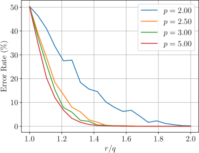
(a) $N_{0}=N_{1}=1500$

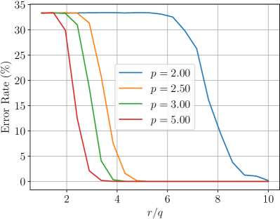
(b) $N_{0}=2000,N_{1}=1000$

Figure 4: Example of the affect of $r/q$ on the classification performance on stochastic block model graphs for various values of $p$.

We present here some numerical results with synthetic and real data, in order to illustrate the main results established in this section, and the room for improvement in future work. The Python code to reproduce the results in this section is available on GitHub.

Our first experiment is with a stochastic block model graph to illustrate Theorem 4.22. We take a graph with $n=3000$ vertices and consider the case of equal block sizes $N_{0}=N_{1}=1500$ and unbalanced block sizes $N_{0}=2000,N_{1}=1000$. We take the intraclass probability to be $r=0.5$, and we vary the interclass probability $q\leq r$. In Figure 4 we show the error rates for binary classification using a labeling rate of $\beta=0.2$ as a function of the ratio $r/q$. For each value of $r/q$ we ran $100$ randomized trials and averaged the error rates. For equal size blocks $N_{0}=N_{1}$, we see that the error rate decreases rapidly when $r/q>1$. Theorem 4.22 guarantees that all vertices are classified correctly when $r/q>\beta^{-1}=5$, which is a pessimistic bound in this case, since all values of $p$ classify correctly when $r/q=2$. For unequal block sizes, $N_{0}/N_{1}=2$ in Figure 4b, we see that for larger values of $p$, the error rate decreases quickly when $r/q>2$, while $p=2$ requires $r/q>8$ to see a similar decrease, and $r/q=10$ to classify correctly. In this case, Theorem 4.22 guarantees correct classification with high probability when $r/q>2\beta^{-1}=10$, which agrees very closely with the $p=2$ result, but is pessimistic for $p>2$. Thus, our results may be tight for $p=2$, but there is clearly much room for improvement in the range $p>2$. In particular, we currently cannot explain why the results in Figure 4b are so dramatically better as $p$ increases. An analysis of this sort would presumably require a different approach to Theorem 4.22 that exploited the tug-of-war game as well.

To illustrate our results on geometric graphs we turn to real data. We consider the MNIST data set which consists of $70000$ images of handwritten digits between $0$ and $9$ [67], with each image a $28\times 28$ grayscale image. We also consider the Cifar-10 data set [65] which contains $60000$ natural images from 10 classes (airplane, automobile, bird, cat, deer, dog, frog, horse, ship, truck). Each Cifar-10 image is a $32\times 32$ pixel color image. To make the problem more similar to our setting, we restrict the data sets from 10 classes down to 2 so we have a binary classification problem. For MNIST we use the 4s and 9s, which are one of the harder pairs of digits to separate, while for Cifar-10 we use the deer and dogs. Figure 5 shows some example images from each data set.

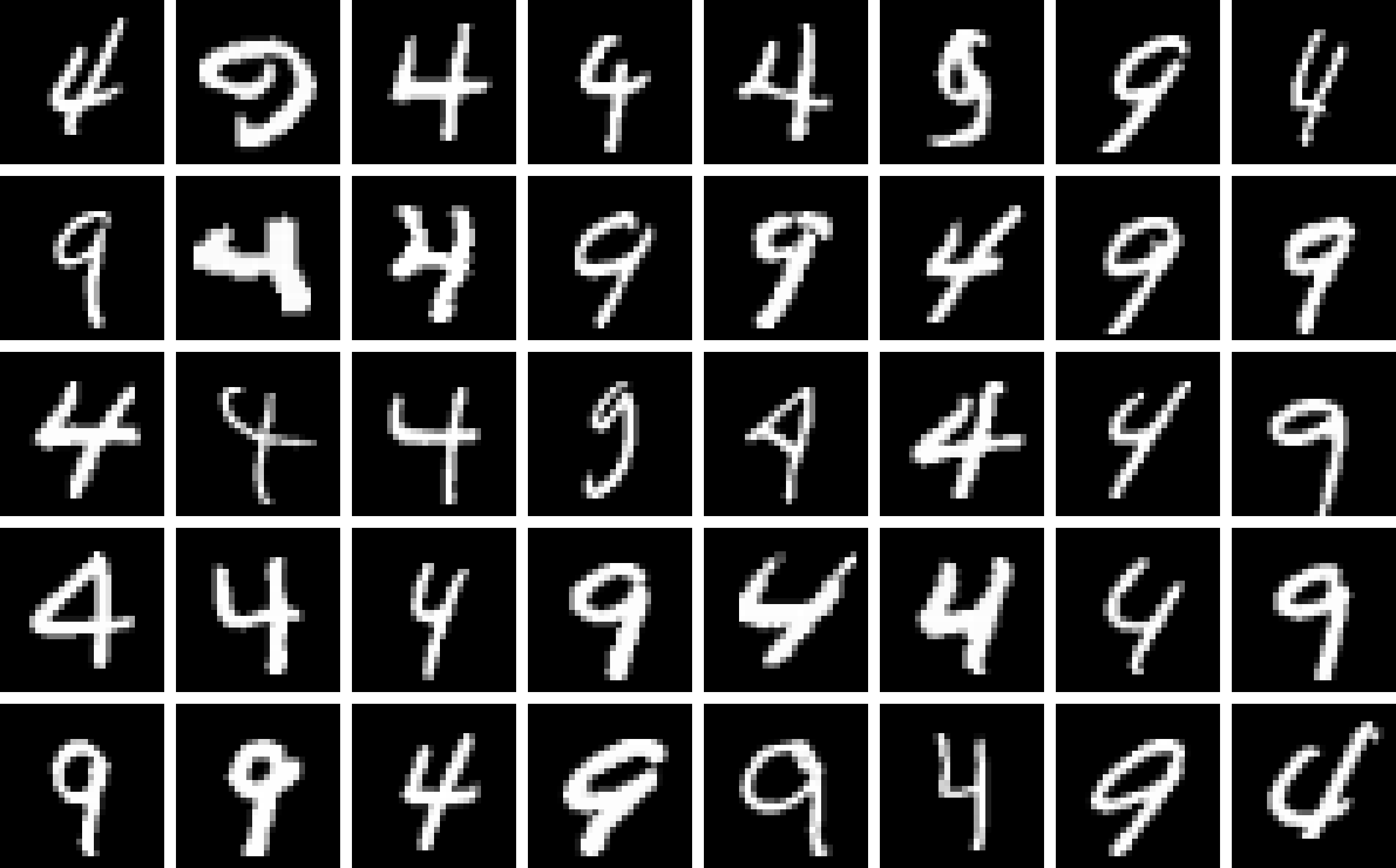
(a) MNIST

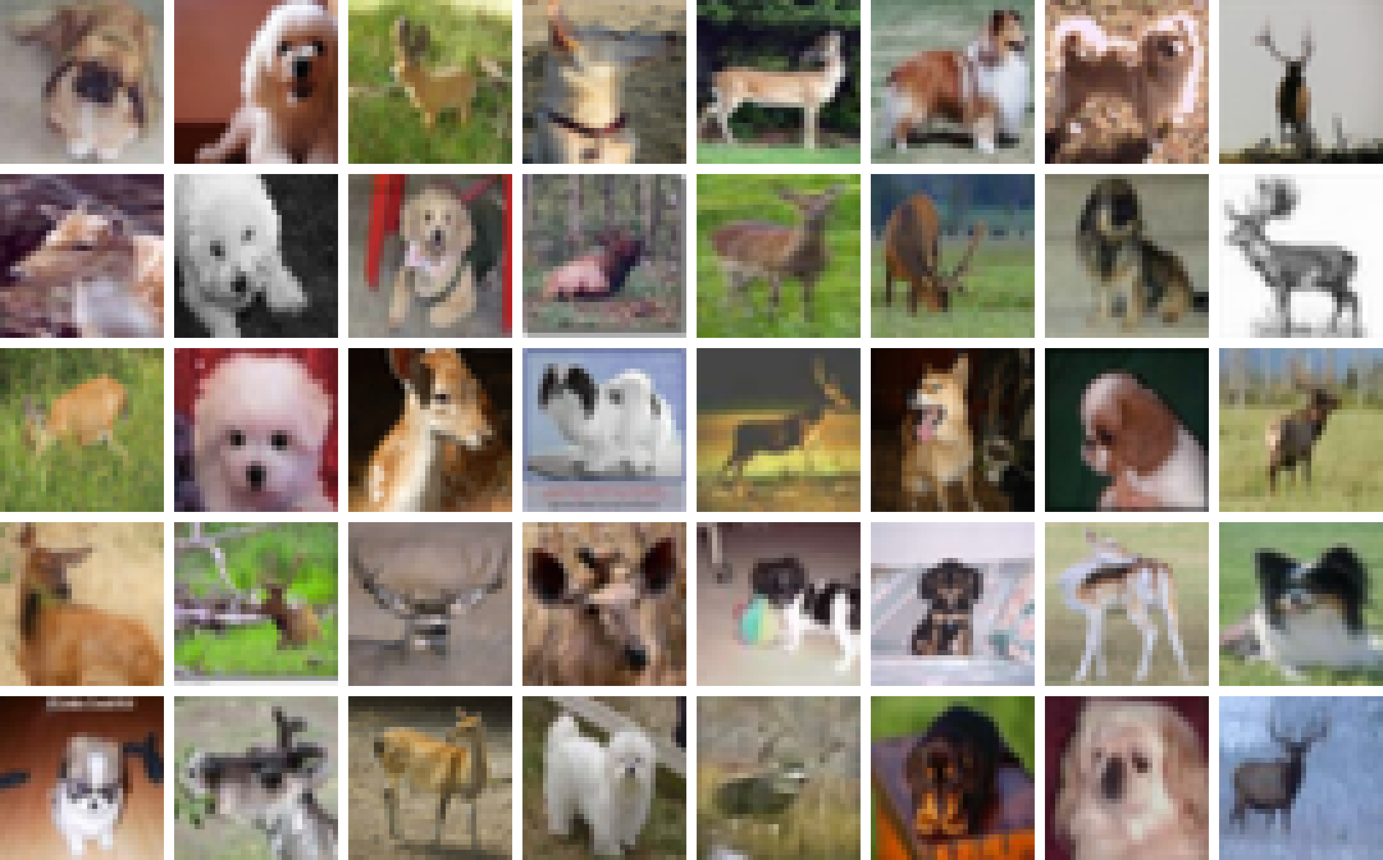
(b) Cifar-10

Figure 5: Sample of MNIST 4s and 9s, and Cifar-10 deer and dogs.

In order to obtain a good feature embedding for constructing the graph, we used a variational autoencoder [63] for MNIST and the contrastive learning SimCLR method [31] for Cifar-10. Both methods are unsupervised deep learning algorithm that learn feature embeddings, or representations, of image data sets that maps the images into a latent space identified with $\mathbb{R}^{k}$ where the similarity in latent features is far more informative of image similarity than pixel-wise similarity. After embedding the images into the feature space, we constructed a $10$ nearest neighbor graph using the angular similarity, as in [22].

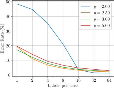
(a) MNIST

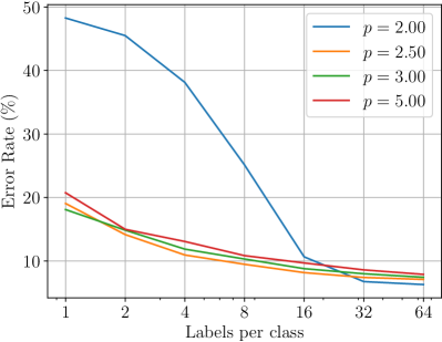
(b) Cifar-10

Figure 6: Accuracy for binary classification of two classes in the MNIST and Cifar-10 data sets using $p$-Laplacian regularization with different values of $p$. We used the 4s and 9s from MNIST, which are one of the more difficult pairs to separate, and the deer and trucks from Cifar-10.

For our experiment we used 1 up to 64 labeled examples per class for each data set, ran 100 trials at each label rate, and reported the average error rate. Figure 6 shows the error rates for different values of $p$ as a function of label rate. We can see that larger values of $p$ give better classification performance at very low label rates, as expected from previous work [44]. Once the label rate is sufficiently large, the error rate becomes small. As predicted in Theorem 4.11, the only points that are misclassified are those that are close to the boundary between classes in terms of graph distance, which are a small fraction of the data points — based on Figure 6 about 2-4% for MNIST and 5-10% for Cifar-10.

5 Conclusions and future work

In this paper, we gave a thorough overview of the intersection between graph-based semi-supervised learning and PDEs, and highlighted problems focused on consistency of classification that have not received significant attention yet in the community. We presented some preliminary results on consistency of $p$-Laplacian based semi-supervised learning. Our results use the stochastic tug-of-war interpretation of the $p$-Laplacian on a graph, and we also provided a brief overview of this field. We proved consistency results for general graphs, geometric graphs, and stochastic block model graphs, the latter of which are not usually covered by continuum PDE-based arguments. One of our findings is that the tug-of-war game transfers nicely between different graph structures, and does not require the geometric structure of the graph. We also presented numerical experiments on synthetic and real data that illustrated our results and suggested directions for future work.

We highlight below some open problems for future work.

1. Relaxing the assumption (A1). The assumption (A1) asks that every vertex on the graph has a labeled neighbor, and is used to make our results tractable. In practice, this means that, in the geometric graph setting, labels do not propagate very far on the graph. It would be very interesting, and more practically relevant, to extend these results to settings where (A1) does not hold. This would require a far more delicate martingale analysis than we provided in this paper.

2. Stochastic block models. Our proof technique in Theorem 4.22 for the stochastic block model graph only exploited the random walk and ignored the tug-of-war component of the game. The numerical results in Section 4.4 suggest that the classification accuracy improves dramatically as $p>2$ increases, even at moderately large label rates — 20% in this case. In order to explain this, it would seem necessary to improve Theorem 4.22 by utilizing the tug-of-war game as well, so that the condition (4.32) on $r/q$ depends on $p$ as well.

3. Extension to other random-walk models. It would be interesting to extend these results to other models that have random walk interpretations, including Poisson learning [22], PWLL [21, 94], and the properly weighted Laplacian [26]. Some of the same high level ideas may work, but we expect many of the ingredients to be different. The case of Laplace learning was essentially already studied in [27].

4. Similar results for other models. There are a number of models that do not have random walk interpretations, such as the variational $p$-Laplacian [36, 107] and the MBO methods [90, 58, 45, 14, 88, 89]. It would be interesting to prove similar consistency results for these methods, though the techniques would be substantially different, since as far as we are aware, there are no representation formulas that express the solutions through stochastic processes in these works.

References

- [1] M. Alamgir and U. V. Luxburg. Phase transition in the family of p-resistances. In Advances in Neural Information Processing Systems, pages 379–387, 2011.
- [2] R. K. Ando and T. Zhang. Learning on graph with Laplacian regularization. In Advances in neural information processing systems, pages 25–32, 2007.
- [3] S. Armstrong and C. Smart. A finite difference approach to the infinity Laplace equation and tug-of-war games. Transactions of the American Mathematical Society, 364(2):595–636, 2012.
- [4] G. Aronsson, M. Crandall, and P. Juutinen. A tour of the theory of absolutely minimizing functions. Bulletin of the American mathematical society, 41(4):439–505, 2004.
- [5] A. Attouchi, H. Luiro, and M. Parviainen. Gradient and Lipschitz estimates for tug-of-war type games. SIAM Journal on Mathematical Analysis, 53(2):1295–1319, 2021.
- [6] A. Azad. Learning Label Initialization for Time-Dependent Harmonic Extension. arXiv preprint arXiv:2205.01358, 2022.
- [7] M. Bardi, I. C. Dolcetta, et al. Optimal control and viscosity solutions of Hamilton-Jacobi-Bellman equations, volume 12. Springer, 1997.
- [8] M. Belkin, I. Matveeva, and P. Niyogi. Regularization and semi-supervised learning on large graphs. In Learning Theory: 17th Annual Conference on Learning Theory, COLT 2004, Banff, Canada, July 1-4, 2004. Proceedings 17, pages 624–638. Springer, 2004.
- [9] M. Belkin and P. Niyogi. Using manifold stucture for partially labeled classification. Advances in neural information processing systems, 15, 2002.
- [10] M. Belkin and P. Niyogi. Laplacian eigenmaps for dimensionality reduction and data representation. Neural computation, 15(6):1373–1396, 2003.
- [11] M. Belkin and P. Niyogi. Semi-supervised learning on Riemannian manifolds. Machine learning, 56:209–239, 2004.
- [12] Y. Bengio, O. Delalleau, and N. Le Roux. Label Propagation and Quadratic Criterion, pages 193–216. MIT Press, semi-supervised learning edition, January 2006.
- [13] S. Boucheron, G. Lugosi, and P. Massart. Concentration Inequalities: A Nonasymptotic Theory of Independence. Univ. Press, 2013.
- [14] Z. M. Boyd, E. Bae, X.-C. Tai, and A. L. Bertozzi. Simplified energy landscape for modularity using total variation. SIAM Journal on Applied Mathematics, 78(5):2439–2464, 2018.
- [15] N. Bridle and X. Zhu. p-voltages: Laplacian regularization for semi-supervised learning on high-dimensional data. In Eleventh Workshop on Mining and Learning with Graphs (MLG2013), 2013.
- [16] J. Brown, R. O’Neill, J. Calder, and A. L. Bertozzi. Utilizing Contrastive Learning for Graph-Based Active Learning of SAR Data. SPIE Defense and Commercial Sensing: Algorithms for Synthetic Aperture Radar Imagery XXX, 2023.
- [17] L. Bungert, J. Calder, and T. Roith. Uniform Convergence Rates for Lipschitz Learning on Graphs. IMA Journal of Numerical Analysis, 2022.
- [18] L. Bungert, J. Calder, and T. Roith. Ratio convergence rates for Euclidean first-passage percolation: Applications to the graph infinity Laplacian. To appear in Annals of Applied Probability, 2023.
- [19] J. Calder. The game theoretic p-Laplacian and semi-supervised learning with few labels. Nonlinearity, 32(1), 2018.
- [20] J. Calder. Consistency of Lipschitz learning with infinite unlabeled data and finite labeled data. SIAM Journal on Mathematics of Data Science, 1(4):780–812, 2019.
- [21] J. Calder, B. Cook, M. Thorpe, D. Slepčev, Y. Zhang, and S. Ke. Graph-Based semi-supervised learning with Poisson equations. In preparation, 2023.
- [22] J. Calder, B. Cook, M. Thorpe, and D. Slepčev. Poisson Learning: Graph based semi-supervised learning at very low label rates. Proceedings of the 37th International Conference on Machine Learning, PMLR, 119:1306–1316, 2020.
- [23] J. Calder and M. Ettehad. Hamilton-Jacobi equations on graphs with applications to semi-supervised learning and data depth. Journal of Machine Learning Research, 23(318):1–62, 2022.
- [24] J. Calder and N. García Trillos. Improved spectral convergence rates for graph Laplacians on -graphs and k-NN graphs. Applied and Computational Harmonic Analysis, 60:123–175, 2022.
- [25] J. Calder, N. García Trillos, and M. Lewicka. Lipschitz regularity of graph Laplacians on random data clouds. SIAM Journal on Mathematical Analysis, 54(1):1169–1222, 2022.
- [26] J. Calder and D. Slepčev. Properly-weighted graph Laplacian for semi-supervised learning. Applied Mathematics and Optimization, 82:1111–1159, 2020.
- [27] J. Calder, D. Slepčev, and M. Thorpe. Rates of convergence for Laplacian semi-supervised learning with low labeling rates. Research in Mathematical Sciences special issue on PDE methods for machine learning, 10(10), 2023.
- [28] O. Chapelle, B. Scholkopf, and A. Zien. Semi-supervised learning. MIT, 2006.
- [29] J. Chapman, B. Chen, Z. Tan, J. Calder, K. Miller, and A. L. Bertozzi. Novel Batch Active Learning Approach and Its Application on the Synthetic Aperture Radar Datasets. SPIE Defense and Commercial Sensing: Algorithms for Synthetic Aperture Radar Imagery XXX (Best Student Paper), 2023.
- [30] F. Charro, J. García Azorero, and J. D. Rossi. A mixed problem for the infinity Laplacian via tug-of-war games. Calculus of Variations and Partial Differential Equations, 34(3):307–320, 2009.
- [31] T. Chen, S. Kornblith, M. Norouzi, and G. Hinton. A simple framework for contrastive learning of visual representations. In International conference on machine learning, pages 1597–1607. PMLR, 2020.
- [32] R. R. Coifman and S. Lafon. Diffusion maps. Applied and computational harmonic analysis, 21(1):5–30, 2006.
- [33] H. Dong, J. Chen, F. Feng, X. He, S. Bi, Z. Ding, and P. Cui. On the equivalence of decoupled graph convolution network and label propagation. In Proceedings of the Web Conference 2021, pages 3651–3662, 2021.
- [34] D. L. Donoho and C. Grimes. Hessian eigenmaps: Locally linear embedding techniques for high-dimensional data. Proceedings of the National Academy of Sciences, 100(10):5591–5596, 2003.
- [35] M. M. Dunlop, D. Slepčev, A. M. Stuart, and M. Thorpe. Large data and zero noise limits of graph-based semi-supervised learning algorithms. Applied and Computational Harmonic Analysis, 49(2):655–697, 2020.
- [36] A. El Alaoui, X. Cheng, A. Ramdas, M. J. Wainwright, and M. I. Jordan. Asymptotic behavior of -based Laplacian regularization in semi-supervised learning. In Conference on Learning Theory, pages 879–906, 2016.
- [37] A. Elmoataz, X. Desquesnes, and M. Toutain. On the game -Laplacian on weighted graphs with applications in image processing and data clustering. European Journal of Applied Mathematics, 28(6):922–948, 2017.
- [38] A. Elmoataz, F. Lozes, and M. Toutain. Nonlocal PDEs on graphs: From tug-of-war games to unified interpolation on images and point clouds. Journal of Mathematical Imaging and Vision, 57(3):381–401, 2017.
- [39] A. Elmoataz, M. Toutain, and D. Tenbrinck. On the -Laplacian and -Laplacian on graphs with applications in image and data processing. SIAM Journal on Imaging Sciences, 8(4):2412–2451, 2015.
- [40] H. Ennaji, Y. Quéau, and A. Elmoataz. Tug of War games and PDEs on graphs with applications in image and high dimensional data processing. Scientific Reports, 13(1):6045, 2023.
- [41] J. Enwright, H. Hardiman-Mostow, J. Calder, and A. L. Bertozzi. Deep semi-supervised label propagation for SAR image classification. SPIE Defense and Commercial Sensing: Algorithms for Synthetic Aperture Radar Imagery XXX, 2023.
- [42] L. Evans. Partial Differential Equations (Graduate Studies in Mathematics, V. 19) GSM/19. American Mathematical Society, June 1998.
- [43] L. C. Evans. A new proof of local C1, regularity for solutions of certain degenerate elliptic pde. Journal of Differential Equations, 45(3):356–373, 1982.
- [44] M. Flores, J. Calder, and G. Lerman. Analysis and algorithms for Lp-based semi-supervised learning on graphs. Applied and Computational Harmonic Analysis, 60:77–122, 2022.
- [45] C. Garcia-Cardona, E. Merkurjev, A. L. Bertozzi, A. Flenner, and A. G. Percus. Multiclass data segmentation using diffuse interface methods on graphs. IEEE transactions on pattern analysis and machine intelligence, 36(8):1600–1613, 2014.
- [46] N. García Trillos, M. Gerlach, M. Hein, and D. Slepčev. Error estimates for spectral convergence of the graph Laplacian on random geometric graphs toward the Laplace–Beltrami operator. Foundations of Computational Mathematics, 20(4):827–887, 2020.
- [47] N. García Trillos and D. Slepčev. Continuum limit of total variation on point clouds. Archive for rational mechanics and analysis, 220:193–241, 2016.
- [48] J. Gasteiger, A. Bojchevski, and S. Günnemann. Predict then Propagate: Graph Neural Networks meet Personalized PageRank. In International Conference on Learning Representations, 2018.
- [49] I. Goodfellow, Y. Bengio, and A. Courville. Deep learning. MIT press, 2016.
- [50] Y. Hafiene, J. Fadili, and A. Elmoataz. Nonlocal -Laplacian Variational problems on graphs. arXiv:1810.12817, 2018.
- [51] J. Ham, D. Lee, and L. Saul. Semisupervised alignment of manifolds. In International Workshop on Artificial Intelligence and Statistics, pages 120–127. PMLR, 2005.
- [52] J. Han. Time-dependent tug-of-war games and normalized parabolic p-Laplace equations. Nonlinear Analysis, 214:112542, 2022.
- [53] J. He, M. Li, H.-J. Zhang, H. Tong, and C. Zhang. Manifold-ranking based image retrieval. In Proceedings of the 12th annual ACM international conference on Multimedia, pages 9–16. ACM, 2004.
- [54] J. He, M. Li, H.-J. Zhang, H. Tong, and C. Zhang. Generalized manifold-ranking-based image retrieval. IEEE Transactions on image processing, 15(10):3170–3177, 2006.
- [55] M. Hein, J.-Y. Audibert, and U. v. Luxburg. Graph Laplacians and their convergence on random neighborhood graphs. Journal of Machine Learning Research, 8(6), 2007.
- [56] M. Hein, J.-Y. Audibert, and U. Von Luxburg. From Graphs to Manifolds-Weak and Strong Pointwise Consistency of Graph Laplacians. In COLT, volume 3559, pages 470–485. Springer, 2005.
- [57] F. Hoffmann, B. Hosseini, A. A. Oberai, and A. M. Stuart. Spectral analysis of weighted Laplacians arising in data clustering. Applied and Computational Harmonic Analysis, 56:189–249, 2022.
- [58] H. Hu, T. Laurent, M. A. Porter, and A. L. Bertozzi. A method based on total variation for network modularity optimization using the MBO scheme. SIAM Journal on Applied Mathematics, 73(6):2224–2246, 2013.
- [59] Q. Huang, H. He, A. Singh, S.-N. Lim, and A. R. Benson. Combining label propagation and simple models out-performs graph neural networks. arXiv preprint arXiv:2010.13993, 2020.
- [60] M. Jacobs, E. Merkurjev, and S. Esedoḡlu. Auction dynamics: A volume constrained MBO scheme. Journal of Computational Physics, 354:288–310, 2018.
- [61] M. Ji and J. Han. A Variance Minimization Criterion to Active Learning on Graphs. In Artificial Intelligence and Statistics, pages 556–564, Mar. 2012.
- [62] A. Jung, A. O. Hero III, A. Mara, and S. Jahromi. Semi-supervised learning via sparse label propagation. arXiv preprint arXiv:1612.01414, 2016.
- [63] D. P. Kingma and M. Welling. Auto-encoding variational bayes. arXiv preprint arXiv:1312.6114, 2013.
- [64] R. Kohn and S. Serfaty. A deterministic-control-based approach motion by curvature. Communications on Pure and Applied Mathematics: A Journal Issued by the Courant Institute of Mathematical Sciences, 59(3):344–407, 2006.
- [65] A. Krizhevsky, G. Hinton, et al. Learning multiple layers of features from tiny images. University of Toronto, 2009.
- [66] R. Kyng, A. Rao, S. Sachdeva, and D. A. Spielman. Algorithms for Lipschitz learning on graphs. In Conference on Learning Theory, pages 1190–1223, 2015.
- [67] Y. LeCun, L. Bottou, Y. Bengio, and P. Haffner. Gradient-based learning applied to document recognition. Proceedings of the IEEE, 86(11):2278–2324, 1998.
- [68] W.-Y. Lee, L.-C. Hsieh, G.-L. Wu, and W. Hsu. Graph-based semi-supervised learning with multi-modality propagation for large-scale image datasets. Journal of visual communication and image representation, 24(3):295–302, 2013.
- [69] G. Leoni. A first course in Sobolev spaces. American Mathematical Soc., 2017.
- [70] M. Lewicka. Random Tug of War games for the p-Laplacian: . arXiv preprint arXiv:1810.03413, 2018.
- [71] M. Lewicka. A course on Tug-of-War games with random noise. Springer, 2020.
- [72] M. Lewicka. Non-local Tug-of-War with noise for the geometric fractional p-Laplacian. Adv. Differential Equations, 27(1-2):31–76, 2022.
- [73] M. Lewicka and J. J. Manfredi. Game theoretical methods in PDEs. Bollettino dell’Unione Matematica Italiana, 7(3):211–216, 2014.
- [74] M. Lewicka and J. J. Manfredi. The obstacle problem for the p-laplacian via optimal stopping of tug-of-war games. Probability Theory and Related Fields, 167:349–378, 2017.
- [75] M. Lewicka and Y. Peres. The Robin mean value equation I: A random walk approach to the third boundary value problem. Potential Analysis, pages 1–32, 2022.
- [76] M. Lewicka and Y. Peres. The Robin mean value equation II: asymptotic Hölder regularity. Potential Analysis, pages 1–35, 2022.
- [77] P. Lindqvist. Notes on the stationary p-Laplace equation. Springer, 2019.
- [78] H. Luiro, M. Parviainen, and E. Saksman. Harnack’s inequality for p-harmonic functions via stochastic games. Communications in Partial Differential Equations, 38(11):1985–2003, 2013.
- [79] U. v. Luxburg and O. Bousquet. Distance-based classification with Lipschitz functions. Journal of Machine Learning Research, 5(Jun):669–695, 2004.
- [80] Y. Ma, R. Garnett, and J. Schneider. -Optimality for Active Learning on Gaussian Random Fields. In C. J. C. Burges, L. Bottou, M. Welling, Z. Ghahramani, and K. Q. Weinberger, editors, Advances in Neural Information Processing Systems 26, pages 2751–2759. Curran Associates, Inc., 2013.
- [81] X. Mai. A random matrix analysis and improvement of semi-supervised learning for large dimensional data. Journal of Machine Learning Research, 19(79):1–27, 2018.
- [82] X. Mai and R. Couillet. Random matrix-inspired improved semi-supervised learning on graphs. In International Conference on Machine Learning, 2018.
- [83] X. Mai and R. Couillet. Consistent semi-supervised graph regularization for high dimensional data. The Journal of Machine Learning Research, 22(1):4181–4228, 2021.
- [84] J. Manfredi, M. Parviainen, and J. Rossi. An asymptotic mean value characterization for p-harmonic functions. Proceedings of the American Mathematical Society, 138(3):881–889, 2010.
- [85] J. J. Manfredi, A. M. Oberman, and A. P. Sviridov. Nonlinear elliptic partial differential equations and p-harmonic functions on graphs. Differential Integral Equations, 28(1-2):79–102, 2015.
- [86] J. J. Manfredi, M. Parviainen, and J. D. Rossi. Dynamic programming principle for tug-of-war games with noise. ESAIM: Control, Optimisation and Calculus of Variations, 18(1):81–90, 2012.
- [87] J. J. Manfredi, M. Parviainen, and J. D. Rossi. On the definition and properties of -harmonious functions. Annali della Scuola Normale Superiore di Pisa-Classe di Scienze, 11(2):215–241, 2012.
- [88] E. Merkurjev, A. L. Bertozzi, and F. Chung. A semi-supervised heat kernel pagerank MBO algorithm for data classification. Communications in Mathematical Sciences, 16(5):1241–1265, 2018.
- [89] E. Merkurjev, C. Garcia-Cardona, A. L. Bertozzi, A. Flenner, and A. G. Percus. Diffuse interface methods for multiclass segmentation of high-dimensional data. Applied Mathematics Letters, 33:29–34, 2014.
- [90] E. Merkurjev, T. Kostic, and A. L. Bertozzi. An MBO scheme on graphs for classification and image processing. SIAM Journal on Imaging Sciences, 6(4):1903–1930, 2013.
- [91] B. Merriman, J. K. Bence, and S. J. Osher. Motion of multiple junctions: A level set approach. Journal of computational physics, 112(2):334–363, 1994.
- [92] K. Miller, X. Baca, J. Mauro, J. Setiadi, Z. Shi, J. Calder, and A. Bertozzi. Graph-based active learning for semi-supervised classification of SAR data. SPIE Defense and Commercial Sensing: Algorithms for Synthetic Aperture Radar Imagery XXIX, 12095, 2022.
- [93] K. Miller and A. L. Bertozzi. Model-change active learning in graph-based semi-supervised learning. arXiv preprint arXiv:2110.07739, 2021.
- [94] K. Miller and J. Calder. Poisson Reweighted Laplacian Uncertainty Sampling for Graph-based Active Learning. To appear in SIAM Journal on Mathematics of Data Science, 2023.
- [95] J. M. Murphy and M. Maggioni. Unsupervised Clustering and Active Learning of Hyperspectral Images With Nonlinear Diffusion. IEEE Transactions on Geoscience and Remote Sensing, 57(3):1829–1845, Mar. 2019.
- [96] B. Nadler, N. Srebro, and X. Zhou. Semi-supervised learning with the graph Laplacian: The limit of infinite unlabelled data. Advances in neural information processing systems, 22:1330–1338, 2009.
- [97] A. Oberman. A convergent difference scheme for the infinity Laplacian: construction of absolutely minimizing Lipschitz extensions. Mathematics of computation, 74(251):1217–1230, 2005.
- [98] A. M. Oberman. Finite difference methods for the infinity Laplace and p-Laplace equations. Journal of Computational and Applied Mathematics, 254:65–80, 2013.
- [99] M. Parviainen. Notes on tug-of-war games and the p-Laplace equation. SpringerBriefs on PDEs and Data Science, 2024.
- [100] Y. Peres, G. Pete, and S. Somersille. Biased tug-of-war, the biased infinity Laplacian, and comparison with exponential cones. Calculus of Variations and Partial Differential Equations, 38(3-4):541–564, 2010.
- [101] Y. Peres, O. Schramm, S. Sheffield, and D. Wilson. Tug-of-war and the infinity Laplacian. Journal of the American Mathematical Society, 22(1):167–210, 2009.
- [102] Y. Peres, S. Sheffield, et al. Tug-of-war with noise: A game-theoretic view of the -Laplacian. Duke Mathematical Journal, 145(1):91–120, 2008.
- [103] Y.-L. Qiao, C. X. Shi, C. Wang, H. Li, M. Haberland, X. Luo, A. M. Stuart, and A. L. Bertozzi. Uncertainty quantification for semi-supervised multi-class classification in image processing and ego-motion analysis of body-worn videos. Image Processing: Algorithms and Systems, 2019.
- [104] P. Sellars, A. I. Aviles-Rivero, and C.-B. Schönlieb. Laplacenet: A hybrid graph-energy neural network for deep semisupervised classification. IEEE Transactions on Neural Networks and Learning Systems, 2022.
- [105] B. Settles. Active learning literature survey. University of Wisconsin-Madison Department of Computer Sciences, 2009.
- [106] Z. Shi, S. Osher, and W. Zhu. Weighted nonlocal Laplacian on interpolation from sparse data. Journal of Scientific Computing, 73(2-3):1164–1177, 2017.
- [107] D. Slepcev and M. Thorpe. Analysis of p-laplacian regularization in semisupervised learning. SIAM Journal on Mathematical Analysis, 51(3):2085–2120, 2019.
- [108] N. G. Trillos, F. Hoffmann, and B. Hosseini. Geometric structure of graph Laplacian embeddings. The Journal of Machine Learning Research, 22(1):2934–2988, 2021.
- [109] U. von Luxburg. A tutorial on spectral clustering. Statistics and Computing, 17(4):395–416, Dec. 2007.
- [110] B. Wang, Z. Tu, and J. K. Tsotsos. Dynamic label propagation for semi-supervised multi-class multi-label classification. In Proceedings of the IEEE international conference on computer vision, pages 425–432, 2013.
- [111] Y. Wang, M. A. Cheema, X. Lin, and Q. Zhang. Multi-manifold ranking: Using multiple features for better image retrieval. In Pacific-Asia Conference on Knowledge Discovery and Data Mining, pages 449–460. Springer, 2013.
- [112] A. Weihs and M. Thorpe. Consistency of Fractional Graph-Laplacian Regularization in Semi-Supervised Learning with Finite Labels. arXiv preprint arXiv:2303.07818, 2023.
- [113] D. Williams. Probability with martingales. Cambridge university press, 1991.
- [114] B. Xu, J. Bu, C. Chen, D. Cai, X. He, W. Liu, and J. Luo. Efficient manifold ranking for image retrieval. In Proceedings of the 34th international ACM SIGIR conference on Research and development in Information Retrieval, pages 525–534. ACM, 2011.
- [115] C. Yang, L. Zhang, H. Lu, X. Ruan, and M.-H. Yang. Saliency detection via graph-based manifold ranking. In Proceedings of the IEEE conference on computer vision and pattern recognition, pages 3166–3173, 2013.
- [116] X. Yang, Z. Song, I. King, and Z. Xu. A survey on deep semi-supervised learning. IEEE Transactions on Knowledge and Data Engineering, 2022.
- [117] D. Zhou, O. Bousquet, T. N. Lal, J. Weston, and B. Schölkopf. Learning with local and global consistency. In Advances in neural information processing systems, pages 321–328, 2004.
- [118] D. Zhou, J. Huang, and B. Schölkopf. Learning from labeled and unlabeled data on a directed graph. In Proceedings of the 22nd international conference on Machine learning, pages 1036–1043. ACM, 2005.
- [119] D. Zhou and B. Schölkopf. Learning from labeled and unlabeled data using random walks. In Joint Pattern Recognition Symposium, pages 237–244. Springer, 2004.
- [120] D. Zhou and B. Schölkopf. Regularization on discrete spaces. In Joint Pattern Recognition Symposium, pages 361–368. Springer, 2005.
- [121] D. Zhou, J. Weston, A. Gretton, O. Bousquet, and B. Schölkopf. Ranking on data manifolds. In Advances in neural information processing systems, pages 169–176, 2004.
- [122] X. Zhou and M. Belkin. Semi-supervised learning by higher order regularization. In Proceedings of the fourteenth international conference on artificial intelligence and statistics, pages 892–900. JMLR Workshop and Conference Proceedings, 2011.
- [123] X. Zhu, Z. Ghahramani, and J. D. Lafferty. Semi-supervised learning using Gaussian fields and harmonic functions. In Proceedings of the 20th International conference on Machine learning (ICML-03), pages 912–919, 2003.
- [124] X. Zhu, J. Lafferty, and Z. Ghahramani. Combining Active Learning and Semi-Supervised Learning Using Gaussian Fields and Harmonic Functions. In International Conference on Machine Learning (ICML) 2003 workshop on The Continuum from Labeled to Unlabeled Data in Machine Learning and Data Mining, pages 58–65, 2003.