Nonproportionality of NaI(Tl) Scintillation Detector for Dark Matter Search Experiments

Abstract

We present a comprehensive study of the nonproportionality of NaI(Tl) scintillation detectors within the context of dark matter search experiments. Our investigation, which integrates COSINE-100 data with supplementary $\gamma$ spectroscopy, measures light yields across diverse energy levels from full-energy $\gamma$ peaks produced by the decays of various isotopes. These $\gamma$ peaks of interest were produced by decays supported by both long and short-lived isotopes. Analyzing peaks from decays supported only by short-lived isotopes presented a unique challenge due to their limited statistics and overlapping energies, which was overcome by long-term data collection and a time-dependent analysis. A key achievement is the direct measurement of the 0.87 keV light yield, resulting from the cascade following electron capture decay of $\rm{{}^{22}Na}$ from internal contamination. This measurement, previously accessible only indirectly, deepens our understanding of NaI(Tl) scintillator behavior in the region of interest for dark matter searches. This study holds substantial implications for background modeling and the interpretation of dark matter signals in NaI(Tl) experiments.

1 Introduction

In 1950, Robert W. Pringle observed that the light output of NaI(Tl) scintillation detector is not proportional to the incident photon energy pringle_gamma-rays_1950 . This discovery sparked numerous studies on nonproportionality (nPR) between light output and the incident electron$/\gamma$ energy using various scintillation detectors engelkemeir_nonlinear_1956 ; aitken_fluorescent_1967 ; leutz_scintillation_1997 ; wayne_response_1998 ; swiderski_response_2013 ; devare_effect_1963 ; collinson_fluorescent_1963 ; jones_nonproportional_1962 . The nPR phenomenon has been observed in various scintillators, including NaI(Tl), but the detailed values were published differently in each experiment. To understand the physics behind the phenomenon and the discrepancies observed, numerous remarkable studies have been published over the decades. These studies include the improvement of measurement techniques khodyuk_nonproportional_2010 ; choong_design_2008 ; choong_performance_2008 ; laplace_simultaneous_2021 as well as theoretical interpretations moses_origins_2012 ; payne_nonproportionality_2009 ; payne_nonproportionality_2011 ; payne_nonproportionality_2014 ; payne_nonproportionality_2015 ; beck_nonproportionality_2015 ; shi_precise_2002 ; dietrich_kinetics_1972 ; rooney_scintillator_1997 ; bizarri_role_2009 ; vasilev_luminescence_2008 ; murray_scintillation_1961 ; li_transport-based_2011 ; li_role_2011 ; kerisit_computer_2009 ; gao_electron-hole_2008 ; kerisit_kinetic_2008 ; bizarri_analytical_2009 , with a subset focusing on simulations.

In recent years, the dark matter (DM) community has shown increasing interest in the nPR of NaI(Tl), particularly in the low-energy region. It is driven by experiments searching for DM using NaI(Tl) detectors, inspired by the observations made by DAMA/LIBRA bernabei_dark_2004 ; bernabei_final_2013 ; b_bernabei_first_2018 . DAMA/LIBRA claimed to have detected an annual modulation signal of DM below 6 keV, which has motivated other experiments to analyze low-energy scintillation events in an attempt to replicate their results adhikari_lowering_2021 ; coarasa_improving_2022 . Moreover, the search for low-mass DM signal in the low-energy region has intensified, with consideration of interactions such as weakly interacting massive particle (WIMP) scattering on the nucleus lee_cosmological_1977 ; goodman_detectability_1985 ; the_cosine-100_collaboration_experiment_2018 ; adhikari_strong_2021 ; adhikari_three-year_2022 ; amare_annual_2021 , the Migdal effect migdal_ionization_1941 ; ibe_migdal_2018 ; cosine-100_collaboration_searching_2022 , and DM-electron scattering cosine-100_collaboration_search_2023 ; the_darkside_collaboration_constraints_2018 ; lee_modulation_2015 ; griffin_extended_2021 ; pandax-ii_collaboration_search_2021 ; essig_direct_2012 ; graham_semiconductor_2012 . Another phenomenon that relies on the analysis of low-energy scintillation is coherent elastic neutrino-nucleus scattering (CE$\nu$NS). Ongoing efforts aim to observe CE$\nu$NS of reactor neutrinos using NaI(Tl) detectors choi_exploring_2023 . Additionally, a feasibility test of future NaI(Tl) detectors for CE$\nu$NS observations of solar and supernova neutrinos has been conducted ko_sensitivities_2023 . These endeavors crucially require understanding extremely low-energy events.

While substantial efforts have been dedicated to lowering the energy threshold through hardware and software upgrades choi_improving_2020 ; lee_scintillation_2022 ; adhikari_lowering_2021 , there has been a relative neglect of the study on nPR of scintillation response. However, misconceptions regarding scintillation response could lead to incorrect interpretations of DM and $\nu$ signals. This is particularly relevant in the low-energy region, where light yield rapidly changes and can introduce significant biases. Unfortunately, previously measured nPR curves have not adequately covered the low-energy region, resulting in a scarcity of reported light-yield measurements at these energies, with only a few indirect or obsolete values available khodyuk_nonproportional_2010 ; aitken_fluorescent_1967 .

To address the aforementioned challenges, this paper presents the results of our $\gamma$-ray calibration of NaI(Tl) crystals used in the COSINE-100 experiment. We utilized various mono-energetic peaks from internally contaminated isotopes, covering an energy range from 0.87 to 88 keV. Given the long-term nature of the DM search experiment, we extracted these energy peaks by simultaneously examining their decay times and peak positions. To complement the data, we also conducted $\gamma$ spectroscopy using another NaI(Tl) crystal from the same manufacturer.

In Sec. 2, we describe the experimental setup, encompassing the COSINE-100 experiment, as well as the additional $\gamma$ spectroscopy. COSINE-100 data, which forms the basis of this study, is summarized in Sec. 3, highlighting the observations and fitting procedures. Sec. 4 focuses on the $\gamma$ spectroscopy methodology, outlining the measurements and analysis techniques to supplement COSINE-100 data. In Sec. 5, we consolidate the results and present the measured nPR. Additionally, we provide the resolution and validate it using a waveform simulation. Finally, in Sec. 6, we conclude by summarizing the key findings of our research and emphasizing the implication for future research.

2 Experimental Setup

The COSINE-100 experiment employed eight high-purity NaI(Tl) crystals, collectively constituting a target for direct DM investigations. These crystals had a total mass of 106 kg and were equipped with one 3-inch photomultiplier tube (PMT) at each of the two ends, enabling the detection of scintillation light. Each crystal was housed within a copper encapsulation. The setup featured eight such encapsulations submerged in a 2,200 L volume of LAB-based liquid scintillator (LS), which served as an active veto system adhikari_cosine-100_2021 . An acrylic box contained the LS, with eighteen PMTs attached to its walls for scintillation light detection, respectively. Events were categorized as multiple-hit or single-hit events based on whether particles left signals in other detectors (LS or crystal). The acrylic box is surrounded by copper and lead, which provide passive shielding layers, while an outermost layer consists of plastic scintillator panels used as a muon veto prihtiadi_muon_2018 .

Signals collected by the crystal PMTs were recorded, as waveforms, through a data acquisition (DAQ) system. The DAQ system comprised pre-amplifiers, analog-to-digital converters (ADC), and a trigger control board (TCB), with detailed specifications outlined in Sec. 7 of Ref. adhikari_initial_2018 . The charge deposition of an event, serving as an indicator of energy, is determined through the integration of the waveform over a 5 $\mu$s time window following noise removal. Data taking for physics purposes commenced on October 20, 2016, at the Yangyang Underground Laboratory adhikari_initial_2018 , and this study utilized data collected through June 9, 2022. Notably, three crystals were excluded from the analysis due to their low light yields or high noise levels the_cosine-100_collaboration_experiment_2018 ; adhikari_three-year_2022 .

Despite the high purity of these NaI(Tl) crystals, radioactive decay signals were observed inside them adhikari_background_2021 . Specifically, in the region of interest of this study, three long-lived isotopes—$\rm{{}^{210}Pb}$, $\rm{{}^{22}Na}$, and $\rm{{}^{40}K}$—were clearly identified as contamination inside the crystals. Moreover, several short-lived isotopes were generated by cosmic rays prior to installation, including $\rm{{}^{109}Cd}$, $\rm{{}^{113}Sn}$, $\rm{{}^{125}I}$, $\rm{{}^{121m}Te}$, and $\rm{{}^{127m}Te}$ barbosa_de_souza_study_2020 . Signal rates from these isotopes were characterized by the isotopes’ decay times and effectively modeled using Monte Carlo simulations. This paper reanalyzes the energy peaks associated with these isotopes, which serve as calibration points.

Apart from the crystals used in COSINE-100, a smaller-sized NaI(Tl) crystal from the same manufacturer was utilized. The crystal had a cylindrical shape with a diameter of 3 inches and a height of 7 inches. It was enveloped in 2–3 mm of PTFE, enclosed by 2 mm of aluminum, and fitted with a quartz window. It featured a 3-inch PMT identical to those used in COSINE-100. The crystal was further shielded using 5-cm-thick lead bricks. The DAQ system for this crystal also included a pre-amplifier, an ADC module, and a TCB, all with the same specifications as those in COSINE-100. Notably, a more stringent trigger condition was applied to reduce the high trigger rate arising from noise and background events at the low-energy region. This setup facilitated measurements of energy responses to external $\gamma$ sources, such as $\rm{{}^{241}Am}$, $\rm{{}^{133}Ba}$, $\rm{{}^{109}Cd}$, and $\rm{{}^{137}Cs}$. Importantly, the peaks used for analysis remained independent of the trigger condition.

3 Extracting Internal Peaks

3.1 Long-Lived Isotopes

The charge distribution of single-hit events in COSINE-100 revealed a distinct peak from $\rm{{}^{210}Pb}$. This peak was modeled with the function $f_{\mathrm{Pb}}(q)$, defined as

$$\begin{split}f_{\mathrm{Pb}}(q)=&\mathrm{Q}\left(q;~{}A,~{}q_{\mathrm{min}},~{}q_{0}\right)\ast\mathrm{N}\left(q;~{}\mu=0,~{}\sigma^{2}\right)\\ &+\mathrm{AG}\left(q;~{}B,~{}\mu,~{}\sigma^{2}_{\mathrm{l}},~{}\sigma^{2}_{\mathrm{r}}\right)+Cq+D,\end{split}$$ (1)

where $q$ is the integrated charge from the signal waveform, while all the other parameters are free fitting parameters. In this equation, the first part ($\mathrm{Q}\ast\mathrm{N}$) represents the 49 keV peak from $\rm{{}^{210}Pb}$, where $\mathrm{Q}$ is the quadratic distribution, defined as

$$\begin{split}\mathrm{Q}&\left(q;~{}A,~{}q_{\mathrm{min}},~{}q_{0}\right)\\ &~{}~{}\equiv\begin{cases}A\left(q-q_{0}\right)^{2},&\text{for }q_{\mathrm{min}}\leq q\leq q_{0}\\ 0,&\text{otherwise}\end{cases},\end{split}$$ (2)

where $A$ is the normalization factor, $q_{0}$ is the vertex position, and $q_{\mathrm{min}}$ is the minimum range of the distribution. This distribution models the sum of $\gamma$ and $\beta$ rays emitted from the $\rm{{}^{210}Pb}$ decay. In this context, $q_{\mathrm{min}}$ represents the charge deposition associated with the energy of the $\gamma$ ray, while $q_{0}$ corresponds to the charge deposition at the maximum total energy. The symbol $\ast$ denotes the convolution operator, and $\mathrm{N}$ is the normal distribution centered at 0 with its standard deviation given by the parameter $\sigma$. The convolution of this normal distribution mimics the resolution-smearing effect in the charge distribution.

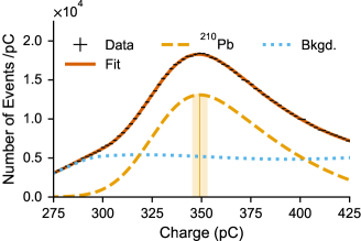
Figure 1: The charge distribution around the 49 keV peak of $\rm{{}^{210}Pb}$, as measured by a NaI(Tl) crystal in COSINE-100 (depicted by the black crosses). The solid red curve represents the fitted model described in Eq. 1. The $\rm{{}^{210}Pb}$ peak is drawn as the dashed yellow curve. The vertical yellow line indicates the position of the $\rm{{}^{210}Pb}$ peak, along with its associated error. The dotted blue curve represents the summed spectrum of background components.

For the background distribution around this peak, we adopted a sum of a linear component ($Cq+D$) and an asymmetric Gaussian distribution $\mathrm{AG}$ defined as

$$\begin{split}\mathrm{AG}&\left(q;~{}B,~{}\mu,~{}\sigma^{2}_{\mathrm{l}},~{}\sigma^{2}_{\mathrm{r}}\right)\\ &~{}\equiv\begin{cases}B\exp{\left[-\left(q-\mu\right)^{2}\,/\,2\sigma^{2}_{l}\right]},&\text{for }q<\mu\\ \\ B\exp{\left[-\left(q-\mu\right)^{2}\,/\,2\sigma^{2}_{r}\right]},&\text{for }q\geq\mu\\ \end{cases},\end{split}$$ (3)

where $B$ is the normalization constant, $\mu$ is the peak position, and $\sigma_{\mathrm{l}}$ and $\sigma_{\mathrm{r}}$ are the standard deviations impacting the left and right tails. These distributions could accurately model the background components. A Monte Carlo simulation was used to verify the fitting procedure, yielding a bias of less than 0.1%. The data distribution and the fitted model are depicted in Fig. 1.

The position of the $\rm{{}^{210}Pb}$ peak was determined as the position where the peak component ($\mathrm{Q}\ast\mathrm{N}$) is maximized. To interpret the position as the light amount for the energy, we assign a 1% systematic uncertainty to account for the unknown spatial distribution of $\rm{{}^{210}Pb}$ within the crystal and for the poorly known spatial dependence of the detector response. The total uncertainty is visually depicted as a yellow band around the vertical line representing the peak position in Fig. 1.

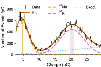
Figure 2: The charge distribution of multiple hit events at the low-energy region, as recorded by a NaI(Tl) crystal in COSINE-100 (indicated by the black crosses). The solid red curve corresponds to the fitted model. Additionally, the dashed yellow curve represents the scaled Poisson distribution for the 0.87 keV from $\rm{{}^{22}Na}$, while the dashed pink curve illustrates the normal distribution for the 3.2 keV from $\rm{{}^{40}K}$. The vertical lines and bands depict their peak positions and associated errors. The dotted blue curve represents the linear-shape model for the background components.

In the charge distribution of multiple-hit events, we observed two distinct peaks associated with isotopes from internal contamination, specifically $\rm{{}^{22}Na}$ and $\rm{{}^{40}K}$. Approximately 10% of $\rm{{}^{22}Na}$ decays to the 1275 keV level of $\rm{{}^{22}Ne}$ through electron capture (EC), while a similar proportion of $\rm{{}^{40}K}$ decays via EC to the 1461 keV level of $\rm{{}^{40}Ar}$ BASUNIA201569 ; CHEN20171 . The daughter atoms undergo cascade processes, leaving characteristic peaks at their respective K-shell edges within the crystal where $\rm{{}^{22}Na}$ and $\rm{{}^{40}K}$ originally resided. Concurrently, high-energy $\gamma$ rays are emitted due to the deexcitation of these daughter nuclei. These energetic $\gamma$ rays can escape the crystal, potentially triggering the neighboring crystals or the LS veto system, leading to coincidences. Consequently, we clearly identified two low-energy peaks in the charge distribution of multiple-hit events, corresponding to 0.87 keV and 3.2 keV. These values represent the K-shell binding energies of $\rm{{}^{22}Ne}$ and $\rm{{}^{40}Ar}$ NISTXray2005 . The charge distribution is shown in Fig. 2, where the observed peak positions and shapes align with our expectations.

For the 0.87 keV peak, a scaled Poisson distribution was used for modeling. The distribution is represented as

$$f_{\mathrm{Na}}\left(q;~{}A,~{}\lambda,~{}s\right)\equiv A\,\frac{\lambda^{q/s}\,e^{-\lambda}}{\Gamma\left(q/s\,+1\right)},$$ (4)

where $A$ is the normalization constant, $\lambda$ is the expected number of photo-electrons ($N_{\mathrm{pe}}$), and $s$ denotes the scaling factor originating from the PMTs. The 3.2 keV peak produced sufficient photo-electrons such that we modeled it using a normal distribution. The background components were attributed to Compton scattering of high-energy external $\gamma$ rays, resulting in relatively smooth shapes. To account for the uncertainty in the background distribution’s shape, flat or linear-shaped distributions were adopted as background models, and the difference between results from these models was considered as a systematic uncertainty. All the parameters denoting the normalization, position, and width of the peaks, and the shape of background distribution are free in the fitting process. The charge distribution, fitted model, and the extracted peak positions are shown in Fig. 2, and the peak positions are summarized in Table 1.

Table 1: List of peak positions extracted from COSINE-100 data.

		Peak Position (pC)
Isotope	Energy (keV)	Crystal 2	Crystal 3	Crystal 4	Crystal 6	Crystal 7
$\rm{{}^{22}Na}$	$0.87$	$5.29\,\pm 0.16$	$5.33\,\pm 0.17$	$4.80\,\pm 0.14$	$5.00\,\pm 0.09$	$5.23\,\pm 0.11$
$\rm{{}^{40}K}$	$3.2$	$21.53\,\pm 0.36$	$21.70\,\pm 0.39$	$20.29\,\pm 0.58$	$19.10\,\pm 0.64$	$20.61\,\pm 0.37$
$\rm{{}^{109}Cd}$	$25$	$192.5\,\pm 2.6$	$198.3\,\pm 2.1$	$183.3\,\pm 1.9$	$165.8\,\pm 2.4$	$177.5\,\pm 2.6$
$\rm{{}^{113}Sn}$	$28$		$223.0\,\pm 3.7$	$202.3\,\pm 2.1$	$190.1\,\pm 2.2$	$201.7\,\pm 2.4$
$\rm{{}^{125}I}$	$39$		$291.7\,\pm 5.4$	$274.1\,\pm 2.8$	$265.6\,\pm 2.8$	$276.5\,\pm 2.9$
$\rm{{}^{210}Pb}$	$49$	$370.7\,\pm 3.7$	$380.1\,\pm 3.8$	$349.2\,\pm 3.5$	$337.0\,\pm 3.4$	$351.7\,\pm 3.5$
$\rm{{}^{125}I}$	$67$		$536.1\,\pm 7.0$	$489.0\,\pm 4.9$	$467.8\,\pm 4.7$	$487.7\,\pm 4.9$
$\rm{{}^{109}Cd}$	$88$	$674.5\,\pm 8.4$	$685.9\,\pm 7.0$	$627.2\,\pm 6.3$	$605.6\,\pm 6.2$	$632.3\,\pm 6.5$

3.2 Short-Lived Isotopes

Short-lived isotopes, such as $\rm{{}^{109}Cd}$, $\rm{{}^{113}Sn}$, $\rm{{}^{125}I}$, $\rm{{}^{121m}Te}$, and $\rm{{}^{127m}Te}$, were initially activated by cosmic rays while the crystals were exposed on the ground and disappeared quickly due to their fast decay times. Their decay processes emit $\gamma$ rays and X-rays at various energy levels, making them valuable for this study. Unfortunately, their energy levels overlap, and their activities are scarce, posing challenges for extracting their peaks using the method outlined in Sec. 3.1. To overcome this issue, we leveraged constraints based on their decay characteristics.

To observe the decays of these isotopes, we accumulated charge distributions over 475 days from the beginning of data acquisition, dividing it into 19 periods, each spanning 25 days. Fig. 3 shows the distributions for three periods: $1^{\mathrm{st}}$, $5^{\mathrm{th}}$, and $9^{\mathrm{th}}$. While decaying and constant components are visually identifiable, determining the position of each peak directly from the spectral shape is challenging. We built a model to extract the peaks from these spectra, with consideration of the decay characteristics of the short-lived isotopes.

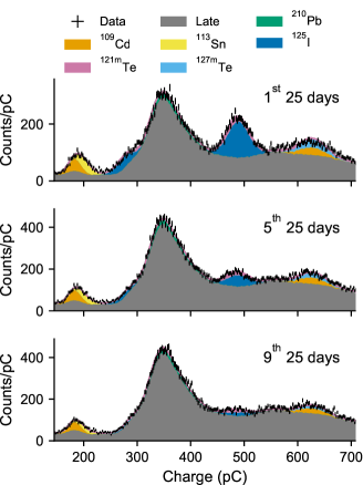
Figure 3: The charge distributions from the initial COSINE-100 data and the extracted peaks attributed to short-lived isotopes. The data points, indicated by black crosses, represent measurements from each data collection period and have been simultaneously fitted by using Eq. 8. The time-normalized late distribution $L(q)$ is depicted as gray histograms in each data collection period. Each isotope component is visualized as a stacked histogram in its own color.

The time-dependent charge distributions for each short-lived isotope $i$ can be expressed as

$$D_{i}\left(q,~{}t;~{}A_{i},~{}\vec{\mu}_{i},~{}\vec{\sigma}_{i}\right)=A_{i}\,e^{-t/\tau_{i}}\sum_{j}f_{ij}\,\mathrm{N}\left(q;~{}\mu_{ij},~{}\sigma^{2}_{ij}\right),$$ (5)

where $t$ denotes time, $A_{i}$ and $\tau_{i}$ are the initial activity and lifetime of isotope $i$, and $f_{ij}$ is the branching fraction for the $j$-th peak of isotope $i$. Each peak is modeled as a normal distribution $\mathrm{N}(q)$ with peak position $\mu_{ij}$ and resolution $\sigma_{ij}$. For the $\rm{{}^{210}Pb}$ component, the normal distribution in Eq. 5 was replaced with $\mathrm{Q}\ast\mathrm{N}$, as used in Sec. 3.1.

The charge distribution accumulated between times $t_{s}$ and $t_{e}$ can be modeled as

$$\begin{split}S&\left(q,~{}t_{s},~{}t_{e};~{}\left\{A_{i},~{}\vec{\mu}_{i},~{}\vec{\sigma}_{i}\right\}\right)\\ &=\int_{t_{s}}^{t_{e}}\left[\sum_{i}D_{i}\left(q,~{}t;~{}A_{i},~{}\vec{\mu}_{i},~{}\vec{\sigma}_{i}\right)+C\left(q\right)\right]s\left(t\right)dt,\end{split}$$ (6)

where $s(t)$ denotes the detector operational state (1 or 0) at time $t$. The term $C(q)$ represents the time-independent component in the spectrum, consisting of isotopes with decay times orders of magnitude longer than the experiment’s duration. Instead of constructing a complex analytic model for the uninteresting $C(q)$ term, we attempted to eliminate its explicit dependence. Since the term is common to all time periods, subtracting a charge distribution from another period with proper time-normalization could effectively remove the $C(q)$ dependency.

For the subtrahend, a late distribution $L(q)$ was accumulated, expressed as $L\left(q\right)=S\left(q,~{}t_{0},~{}t_{1}\right)$ for $t_{0}$ and $t_{1}$ defined as 650 days and 1,150 days after the start of data acquisition. Due to its long time period, $L(q)$ has a sufficiently small error to be treated in the model as a known distribution rather than fitted data. Replacing the $C(q)$ term with $L(q)$ from Eq. 6 yields

$$\begin{split}S&\left(q,~{}t_{s},~{}t_{e};~{}\left\{A_{i},~{}\vec{\mu}_{i},~{}\vec{\sigma}_{i}\right\}\right)\\ &=\int_{t_{s}}^{t_{e}}\sum_{i}D_{i}\left(q,~{}t\right)\,s\left(t\right)\,dt\\ &~{}~{}~{}~{}+\frac{\int_{t_{s}}^{t_{e}}s(t)\,dt}{\int_{t_{0}}^{t_{1}}s(t)\,dt}\left[L\left(q\right)-\int_{t_{0}}^{t_{1}}\sum_{i}D_{i}\left(q,~{}t\right)\,s\left(t\right)\,dt\right],\end{split}$$ (7)

which depends only on the set of parameters related to the peaks. Consequently, the number of events for the $k$-th 25-days-period spectrum in the $l$-th charge bin is expected as $S_{kl}=S\left(q_{l},~{}(k-1)\Delta T,~{}k\Delta T\right)$, where $q_{l}$ is the central value of the $l$-th charge bin, and $\Delta T$ is the period interval, 25 days.

To extract peaks from the short-lived isotopes, we conducted a simultaneous fit on 19 distributions using a binned likelihood,

$$\begin{split}\mathcal{L}&\left(\left\{A_{i},\vec{\mu}_{i},~{}\vec{\sigma}_{i}\right\};~{}\mathbf{O},~{}\vec{\mu}^{A},~{}\vec{\sigma}^{A}\right)\\ &=\prod_{k}^{19}\prod_{l}^{N_{\mathrm{bin}}}\frac{S_{kl}^{O_{kl}}e^{-S_{kl}}}{O_{kl}!}\times\prod_{i}\exp\left[-\frac{1}{2}\left(\frac{A_{i}-\mu_{i}^{A}}{\sigma_{i}^{A}}\right)^{2}\right],\end{split}$$ (8)

where $O_{kl}$ is the observed number of events in the $k$-th period spectrum at the $l$-th charge bin. The initial activity $A_{i}$, peak positions $\mu_{ij}$, and resolutions $\sigma_{ij}$ were treated as free parameters, while those for $\rm{{}^{210}Pb}$ were kept constant at the values obtained in Sec. 3.1. Constraints for the initial activities, $\mu^{A}_{i}$ and $\sigma^{A}_{i}$ were obtained from our previous measurement barbosa_de_souza_study_2020 . As seen in Fig. 3, the extracted peaks effectively account for the charge distributions in different time domains simultaneously. For verification, we applied the same fitting procedure to simulated distributions, allowing us to obtain the true mean energy value for each peak. Through this process, light yields were obtained for several points ranging from 25 to 88 keV, as summarized in Table 1.

4 Gamma Spectroscopy

An independent experiment was conducted for $\gamma$ spectroscopy to acquire complementary data and broaden the energy range of our analysis. Charge distributions were measured using four $\gamma$ sources, $\rm{{}^{241}Am}$, $\rm{{}^{133}Ba}$, $\rm{{}^{109}Cd}$, and $\rm{{}^{137}Cs}$. These sources were placed near the crystal and aligned at its center during data taking. The energies of the $\gamma$ rays and X-rays emitted from these sources, along with their exposure times, are listed in Table 2. Data without any sources was also collected over an extended period to obtain the background distributions before and after acquiring data with the sources. This allowed us to verify the stability of the PMT gain and background distribution with time. The pure peak for each source was identified by subtracting the background distribution, as illustrated in Fig 4.

Table 2: List of sources used for $\gamma$ spectroscopy, with measured peak positions.

$\gamma$ Source	Time	Energy	Peak Position
	(Hours)	(keV)	(pC)
No Source	22
$\rm{{}^{241}Am}$	14	$59.25\,\pm 0.16$	$453.4\,\pm 4.4$
$\rm{{}^{133}Ba}$	6	$29.17\,\pm 0.08$	$211.5\,\pm 2.2$
		$30.82\,\pm 0.08$	$224.1\,\pm 2.2$
		$35.73\,\pm 0.10$	$251.4\,\pm 2.6$
		$51.65\,\pm 0.14$	$375.7\,\pm 3.8$
		$80.00\,\pm 0.22$	$588.8\,\pm 5.9$
$\rm{{}^{109}Cd}$	8	$21.98\,\pm 0.06$	$157.5\,\pm 1.6$
		$24.63\,\pm 0.07$	$177.8\,\pm 1.8$
		$87.54\,\pm 0.24$	$641.3\,\pm 6.8$
$\rm{{}^{137}Cs}$	11	$32.11\,\pm 0.10$	$234.5\,\pm 2.4$
		$37.54\,\pm 0.30$	$268.9\,\pm 4.2$

The peak positions were determined by fitting the charge distributions. The charge distribution for isotope $i$ can be modeled as

$$S_{i}\left(q\right)=\sum_{j}N_{ij}\,\mathrm{CB}\left(q;~{}\mu_{ij},~{}\sigma_{ij},~{}\alpha_{ij},~{}n_{ij}\right),$$ (9)

where $N_{ij}$ represents the normalization constant of the $j$-th peak, and $\mathrm{CB}(q)$ denotes a Crystal Ball function commonly used to model peaks measured by scintillation crystals with energy loss processes gaiser_charmonium_1982 . The function includes parameters for peak position $\mu_{ij}$ and resolution $\sigma_{ij}$, which are free during the fitting process. The $\alpha_{ij}$ and $n_{ij}$ parameters account for the peak shape. Flat and linear background components were added to the $\rm{{}^{133}Ba}$ and $\rm{{}^{137}Cs}$ distributions, respectively, to model Compton scattering of high-energy $\gamma$ rays.

Figure 4: Charge distributions of external sources after subtraction of the background distribution, recorded by the sample crystal for $\gamma$ spectroscopy. Black crosses represent the data, and red curves depict the fitting results used to extract the peak positions. The peak positions extracted are shown as vertical lines with error bands.

The model was fitted to data by minimizing the following chi-squared:

$$\chi^{2}_{i}\equiv\sum_{l}^{N_{\mathrm{bin}}}\dfrac{\left[D_{il}-\left(t_{i}/t_{b}\right)B_{l}-S_{i}\left(q_{l}\right)\right]^{2}}{D_{il}+\left(t_{i}/t_{b}\right)^{2}B_{l}}.$$ (10)

In this equation, $D_{i}l$ and $B_{l}$ are the measured number of events in $i$-th source and background data, respectively, at the $l$-th charge bin, centered at $q_{l}$. Exposure times for the $i$-th source and background data are represented by $t_{i}$ and $t_{b}$, respectively. The extracted peak positions are displayed in Fig. 4 as vertical lines with their uncertainties.

The same fitting procedure was conducted as in Sec. 3, with distributions obtained by GEANT4 Monte Carlo simulation agostinelli_geant4simulation_2003 . All dimensions of the detector geometry were implemented based on measurements, except for the thickness of the PTFE wrapped inside the aluminum case. To account for the uncertainty, two different conditions were simulated with this thicknesses set to 2 mm and 3 mm. The simulation results were fitted separately, and the difference in peak positions was assigned to the systematic error of the true energy. One can see those errors and the extracted peak positions in Table 2.

5 Scintillation Response of NaI(Tl) Crystal

5.1 Photon Response Measurements

The relative light yield obtained via peak extraction is depicted in Fig. 5. Both the response function and the data points are normalized to the value at 50 keV to highlight the nonproportional behavior of the light yield. The error bars include systematic errors resulting from the radioactive source’s position and the peak extraction method. These measurements exhibited consistency across the crystals and the measuring techniques within the associated uncertainties. The well-known K-shell dip of NaI(Tl) at 33 keV is also identifiable.

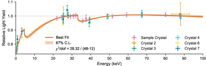
Figure 5: The relative light yield as a function of incident $\gamma$-ray energy, normalized to the value at 50 keV. The measurements are represented by colored dots with error bars, and the fitted function is drawn as the red curve. The translucent red band represents the uncertainty from the modeling at 67% confidence level.

The data was fitted using an empirical function developed based on the Payne’s model payne_nonproportionality_2009 ; payne_nonproportionality_2011 ; payne_nonproportionality_2014 ; payne_nonproportionality_2015 ; beck_nonproportionality_2015 , as shown by the red curve in Fig. 5. An expectation arises for the presence of the L-shell dip structure around 4.5 keV, although there is an insufficient number of data points below 20 keV to constrain the detailed shape of the dip. We have checked the consistency of our curve with measurements from two references comparing quantities, such as the light-yield ratio between 4.5 and 20 keV, the ratio between 0.87 and 20 keV, and the slope around 10 keV. These were found to be consistent with previous reports khodyuk_nonproportional_2010 ; aitken_fluorescent_1967 , as summarized in Table 3. Despite this consistency check, we acknowledge that our curve between 4.5 and 20 keV is less convincing, resulting in a relatively wider error band, with its width dependent on the selected model parameterization. The measurement of light yield in this energy region is left for future investigation.

Table 3: Comparison of $\gamma$ nPR measurements khodyuk_nonproportional_2010 ; aitken_fluorescent_1967 . $\mathrm{LY}_{\gamma}\left(E\right)$ is the light yield for a $\gamma$ ray with incident energy $E$, and $\mathrm{LY}_{\gamma,~{}50}\left(E\right)\equiv\mathrm{LY}_{\gamma}\left(E\right)/\mathrm{LY}_{\gamma}\left(50\,\mathrm{keV}\right)$.

	This Work	Khodyuk	Aitken
$\dfrac{d\,\mathrm{LY}_{\gamma,~{}50}}{dE}\left(10\,\mathrm{keV}\right)$ $\left(\dfrac{\%}{\mathrm{keV}}\right)$	1.12	1.18	1.16
$\dfrac{\mathrm{LY}_{\gamma}\left(4.5\,\mathrm{keV}\right)}{\mathrm{LY}_{\gamma}\left(20\,\mathrm{keV}\right)}$ (%)	93.0	93.3	91.8
$\dfrac{\mathrm{LY}_{\gamma}\left(0.89\,\mathrm{keV}\right)}{\mathrm{LY}_{\gamma}\left(20\,\mathrm{keV}\right)}$ (%)	83.7	89.3

To evaluate the nPR in the high-energy region above 200 keV, we examined its consistency with the data reported in Ref. devare_effect_1963 . We measured the light yields by fitting the prominent $\gamma$ peaks from the high-energy spectrum, including 295 keV from $\rm{{}^{214}Pb}$, 511 and 1274 keV from $\rm{{}^{22}Na}$, 609 and 1764 keV from $\rm{{}^{214}Bi}$, 1461 keV from $\rm{{}^{40}K}$, and 2615 keV from $\rm{{}^{208}Tl}$. The measured light yields demonstrate agreement with the nPR curve reported in Ref. devare_effect_1963 , as illustrated in Fig. 6.

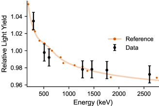
Figure 6: The relative light yield (normalized at 662 keV) for the high-energy $\gamma$ peaks is represented by black dots with error bars. The red dots and curve represent the nPR measured from Ref. devare_effect_1963 , where our data agrees well with the reference.

5.2 Resolution and Waveform Simulation

Once a peak is extracted, the energy resolution $\sigma_{ij}$ is naturally obtained along with the peak position $\mu_{ij}$. As shown in the dashed gray curve in Fig. 7, the characteristic $1/\sqrt{E}$-like shape, originating from the Poisson fluctuations in $N_{\mathrm{pe}}$ for the PMT, is clearly visible. Also resolution effects due to the detector geometry and the distribution of the number of amplified electrons in the PMT are observed.

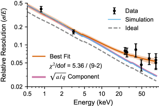
Figure 7: The relative resolution as a function of incident $\gamma$-ray energy for a NaI(Tl) crystal. The black dots with error bars represent the measurements, and the red curve represents the model of the resolution curve, as described in Eq. 11, with an error band at 67% confidence level. The solid pink curve illustrates the $\sqrt{a/q}$ component from the resolution model, which closely matches the waveform simulation (solid blue curve). The dashed gray curve represents the Poisson fluctuation in $N_{\mathrm{pe}}$.

To account for these effects, the relative resolution as a function of charge was modeled using the following equation,

$$\frac{\sigma(q)}{q}=\sqrt{\frac{a}{q}+b}.$$ (11)

Here, $a$ and $b$ are fitting parameters, where $a$ scales the Poisson resolution contribution and $b$ typically arises from non-uniformity of detector response, which is not included in the simulation. In Fig. 7, the red line represents the model fitted to the measurements, with the uncertainty shown as a band. The resolution $\sigma(q)$ is transformed to $\sigma(E)$ via the nPR curve shown in Fig. 5, leading to the emergence of non-analytic points at the 4 keV L-shell edge and the 33 keV K-shell edge. The pink line represents the function when $b=0$.

Given the focus on DM detection experiments, where the region of interest typically lies below 6 keV, it is crucial to investigate the resolution in the sub-keV range, particularly for future upgrades. Since the effect of electron amplification in PMTs and DAQ system is most dominant at low energies, except for that due to the Poisson fluctuations with $N_{\mathrm{pe}}$, a waveform simulation developed for the COSINE-100 experiment was utilized to validate the resolution in this region. This simulation incorporates factors such as rise and decay times of NaI(Tl) scintillation, fluctuations in the single photo-electron shape, DAQ electronics, and charge accumulation processes. Therefore, by inputting $N_{\mathrm{pe}}$ that takes into account Poisson fluctuations, we can estimate the resolution with these effects included.

The blue line in Fig. 7 shows that the simulation successfully replicates the data. Despite not accounting for the intricate details of detector geometry and other mechanisms, the simulation exhibits good agreement with the measurements at the low-energy region. In addition, the agreement between the simulation and the pink curve, which is the measurement with the constant-term factor excluded, confirms the possibility of extrapolating the resolution curve to the low-energy direction. These findings hold particular significance for scintillator experiments focusing on low-energy ranges.

6 Summary and Conclusion

In conclusion, this study has thoroughly examined the nPR characteristics of NaI(Tl) scintillators within the context of DM search experiments. Through a comprehensive calibration process using COSINE-100 data, complemented by $\gamma$ spectroscopy, we have gained valuable insights into the behavior of NaI(Tl) crystals.

The measurement of light yields at various energies was successfully achieved by analyzing internal peaks originating from both long-lived and short-lived isotopes. Extraction of peaks from long-lived isotopes was easily accomplished due to stable experimental data acquisition. A significant milestone was reached by directly measuring the light yield at 0.87 keV, generated by the cascade following $\rm{{}^{22}Na}$ EC decay, facilitated by the active veto system. This direct measurement serves as validation of an indirect measurement obtained by analyzing X-rays near the Iodine K-shell using synchrotron radiation khodyuk_nonproportional_2010 . Overcoming the challenge of extracting multiple overlaid peaks from short-lived isotopes was made possible through long-term data collection and time-dependent analysis.

In the nPR curve measured here, the distinctive K-shell dip structure was observed. The nPR curve was fitted using an empirical curve. The resulting fitted nPR curve exhibits consistency with previously reported measurements, particularly in the energy range below 20 keV. However, the lack of data points around the 10 keV region limits the precision of the calibration curve, leaving the error band relatively wider. This aspect remains a focus for future investigation.

The resolution analysis of NaI(Tl) scintillators revealed a characteristic resolution curve that follows the $1/\sqrt{N_{\mathrm{pe}}}$ trend, as expected for Poisson fluctuations in $N_{\mathrm{pe}}$. Waveform simulation provided compelling confirmation of the resolution at low energies, allowing for the extension of the resolution curve to lower energy ranges. This enhancement in our ability to detect low-energy DM recoil signals is very important.

The findings of this study hold significant implications for background modeling in NaI(Tl) experiments. Precise calibration and characterization of the nPR effect are essential for accurately modeling the background spectra resulting from radioactive interactions involving electrons and photons. To facilitate more detailed simulations, the integration of the nonproportional light production of NaI(Tl) into the GEANT4 toolkit is under development, building on similar efforts reported previously rasco_nonlinear_2015 ; cano-ott_monte_1999 .

Furthermore, it is imperative to consider nPR calibration when interpreting signals that may come from DM interactions with electrons or photons. As the scientific community explores diverse scenarios involving boosted DM and light DM, the significance of these interactions is poised to grow. This study lays the foundation for more robust and accurate DM search experiments in the future.

- (1) R. W. Pringle and S. Standil, The Gamma-Rays from Neutron-Activated Gold, Phys. Rev. 80, 762–763 (1950).
- (2) D. Engelkemeir, Nonlinear Response of NaI(Tl) to Photons, Rev. Sci. Instrum. 27, 589–591 (1956).
- (3) D. W. Aitken et al., The Fluorescent Response of NaI(Tl), CsI(Tl), CsI(Na) and CaF2(Eu) to X-Rays and Low Energy Gamma Rays, IEEE Trans. Nucl. Sci. 14, 468–477 (1967).
- (4) H. Leutz and C. D’Ambrosio, On the scintillation response of NaI(TI)-crystals, IEEE Trans. Nucl. Sci. 44, 190–193 (1997).
- (5) L. R. Wayne et al., Response of NaI(Tl) to X-rays and electrons, Nucl. Instrum. Methods Phys. Res. Sect. A 411, 351–364 (1998).
- (6) L. Swiderski et al., Response of doped alkali iodides measured with gamma-ray absorption and Compton electrons, Nucl. Instrum. Methods Phys. Res. Sect. A 705, 42–46 (2013).
- (7) H. G. Devare and P. N. Tandon, Effect of the non-linear response of NaI(Tl) on the single crystal summing spectra, Nucl. Instrum. Methods 22, 253–255 (1963).
- (8) A. J. L. Collinson and R. Hill, The Fluorescent Response of NaI(Tl) and CsI(Tl) to X Rays and Rays, Proc. Phys. Soc. 81, 883 (1963).
- (9) T. H. Jones, The nonproportional response of a NaI(Tl) crystal to diffracted X rays, Nucl. Instrum. Methods 15, 55–58 (1962).
- (10) I. V. Khodyuk, P. A. Rodnyi, and P. Dorenbos, Nonproportional scintillation response of NaI:Tl to low energy x-ray photons and electrons, J. Appl. Phys. 107, 113513 (2010).
- (11) W.-S. Choong et al., Design of a Facility for Measuring Scintillator Non-Proportionality, IEEE Trans. Nucl. Sci. 55, 1753–1758 (2008).
- (12) W.-S. Choong et al., Performance of a Facility for Measuring Scintillator Non-Proportionality, IEEE Trans. Nucl. Sci. 55, 1073–1078 (2008).
- (13) T. A. Laplace et al., Simultaneous measurement of organic scintillator response to carbon and proton recoils, Phys. Rev. C 104, 014609 (2021).
- (14) W. W. Moses et al., The Origins of Scintillator Non-Proportionality, IEEE Trans. Nucl. Sci. 59, 2038–2044 (2012).
- (15) S. A. Payne et al., Nonproportionality of Scintillator Detectors: Theory and Experiment, IEEE Trans. Nucl. Sci. 56, 2506–2512 (2009).
- (16) S. A. Payne et al., Nonproportionality of Scintillator Detectors: Theory and Experiment. II, IEEE Trans. Nucl. Sci. 58, 3392–3402 (2011).
- (17) S. A. Payne et al., Nonproportionality of Scintillator Detectors. III. Temperature Dependence Studies, IEEE Trans. Nucl. Sci. 61, 2771–2777 (2014).
- (18) S. A. Payne, Nonproportionality of Scintillator Detectors. IV. Resolution Contribution from Delta-Rays, IEEE Trans. Nucl. Sci. 62, 372–380 (2015).
- (19) P. R. Beck et al., Nonproportionality of Scintillator Detectors. V. Comparing the Gamma and Electron Response, IEEE Trans. Nucl. Sci. 62, 1429–1436 (2015).
- (20) H.-X. Shi et al., Precise Monte Carlo simulation of gamma-ray response functions for an NaI(Tl) detector, Appl. Radiat. Isot. 57, 517–524 (2002).
- (21) H. B. Dietrich and R. B. Murray, Kinetics of the diffusion of self-trapped holes in alkali halide scintillators, J. Luminescence 5, 155–170 (1972).
- (22) B. Rooney and J. Valentine, Scintillator light yield nonproportionality: calculating photon response using measured electron response, IEEE Trans. Nucl. Sci. 44, 509–516 (1997).
- (23) G. Bizarri et al., The role of different linear and non-linear channels of relaxation in scintillator non-proportionality, J. Luminescence 129, 1790–1793 (2009).
- (24) A. N. Vasil’ev, From Luminescence Non-Linearity to Scintillation Non-Proportionality, IEEE Trans. Nucl. Sci. 55, 1054–1061 (2008).
- (25) R. B. Murray and A. Meyer, Scintillation Response of Activated Inorganic Crystals to Various Charged Particles, Phys. Rev. 122, 815–826 (1961).
- (26) Q. Li et al., A transport-based model of material trends in nonproportionality of scintillators, J. Appl. Phys. 109, 123716 (2011).
- (27) Q. Li et al., The role of hole mobility in scintillator proportionality, Nucl. Instrum. Methods Phys. Res. Sect. A 652, 288–291 (2011).
- (28) S. Kerisit et al., Computer simulation of the light yield nonlinearity of inorganic scintillators, J. Appl. Phys. 105, 114915 (2009).
- (29) F. Gao et al., Electron-Hole Pairs Created by Photons and Intrinsic Properties in Detector Materials, IEEE Trans. Nucl. Sci. 55, 1079–1085 (2008).
- (30) S. Kerisit, K. M. Rosso, and B. D. Cannon, Kinetic Monte Carlo Model of Scintillation Mechanisms in CsI and CsI(Tl), IEEE Trans. Nucl. Sci. 55, 1251–1258 (2008).
- (31) G. Bizarri et al., An analytical model of nonproportional scintillator light yield in terms of recombination rates, J. Appl. Phys. 105, 044507 (2009).
- (32) R. Bernabei et al., (DAMA/NaI), Dark Matter Particles in the Galactic Halo: Results and Implications from dama/nai, Int. J. Mod. Phys. D 13, 2127–2159 (2004).
- (33) R. Bernabei et al., (DAMA/LIBRA), Final model independent result of DAMA/LIBRA–phase1, Eur. Phys. J. C 73, 2648 (2013).
- (34) B. Bernabei et al., (DAMA/LIBRA), First model independent results from DAMA/LIBRA-phase2, Nucl. Phys. At. Energy 19, 307–325 (2018).
- (35) G. Adhikari et al., (COSINE-100), Lowering the energy threshold in COSINE-100 dark matter searches, Astropart. Phys. 130, 102581 (2021).
- (36) I. Coarasa et al., (ANAIS-112), Improving ANAIS-112 sensitivity to DAMA/LIBRA signal with machine learning techniques, J. Cosmol. Astropart. Phys. 2022, 048 (2022).
- (37) B. W. Lee and S. Weinberg, Cosmological Lower Bound on Heavy-Neutrino Masses, Phys. Rev. Lett. 39, 165–168 (1977).
- (38) M. W. Goodman and E. Witten, Detectability of certain dark-matter candidates, Phys. Rev. D 31, 3059–3063 (1985).
- (39) G. Adhikari et al., (COSINE-100), An experiment to search for dark-matter interactions using sodium iodide detectors, Nature 564, 83–86 (2018).
- (40) G. Adhikari et al., (COSINE-100), Strong constraints from COSINE-100 on the DAMA dark matter results using the same sodium iodide target, Sci. Adv. 7, eabk2699 (2021).
- (41) G. Adhikari et al., (COSINE-100), Three-year annual modulation search with COSINE-100, Phys. Rev. D 106, 052005 (2022).
- (42) J. Amaré et al., (ANAIS-112), Annual modulation results from three-year exposure of ANAIS-112, Phys. Rev. D 103, 102005 (2021).
- (43) A. Migdal, Ionization of atoms accompanying -and -decay, J. Phys. USSR 4, 449 (1941).
- (44) M. Ibe et al., Migdal effect in dark matter direct detection experiments, J. High Energ. Phys. 2018, 194 (2018).
- (45) G. Adhikari et al., (COSINE-100), Searching for low-mass dark matter via the Migdal effect in COSINE-100, Phys. Rev. D 105, 042006 (2022).
- (46) G. Adhikari et al., (COSINE-100), Search for solar bosonic dark matter annual modulation with COSINE-100, Phys. Rev. D 107, 122004 (2023).
- (47) P. Agnes et al., (DarkSide), Constraints on Sub-GeV Dark-Matter–Electron Scattering from the DarkSide-50 Experiment, Phys. Rev. Lett. 121, 111303 (2018).
- (48) S. K. Lee et al., Modulation effects in dark matter-electron scattering experiments, Phys. Rev. D 92, 083517 (2015).
- (49) S. M. Griffin et al., Extended calculation of dark matter-electron scattering in crystal targets, Phys. Rev. D 104, 095015 (2021).
- (50) C. Cheng et al., (PandaX-II), Search for Light Dark Matter–Electron Scattering in the PandaX-II Experiment, Phys. Rev. Lett. 126, 211803 (2021).
- (51) R. Essig, J. Mardon, and T. Volansky, Direct detection of sub-GeV dark matter, Phys. Rev. D 85, 076007 (2012).
- (52) P. W. Graham et al., Semiconductor probes of light dark matter, Phys. Dark Universe 1, 32–49 (2012).
- (53) J. J. Choi et al., (NEON), Exploring coherent elastic neutrino-nucleus scattering using reactor electron antineutrinos in the NEON experiment, Eur. Phys. J. C 83, 226 (2023).
- (54) Y. J. Ko and H. S. Lee, Sensitivities for coherent elastic scattering of solar and supernova neutrinos with future NaI(Tl) dark matter search detectors of COSINE-200/1T, Astropart. Phys. 153, 102890 (2023).
- (55) J. J. Choi et al., (NEON), Improving the light collection using a new NaI(Tl) crystal encapsulation, Nucl. Instrum. Methods Phys. Res. Sect. A 981, 164556 (2020).
- (56) H. Y. Lee et al., Scintillation characteristics of a NaI(Tl) crystal at low-temperature with silicon photomultiplier, J. Inst. 17, P02027 (2022).
- (57) G. Adhikari et al., (COSINE-100), The COSINE-100 liquid scintillator veto system, Nucl. Instrum. Methods Phys. Res. Sect. A 1006, 165431 (2021).
- (58) H. Prihtiadi et al., (COSINE-100), Muon detector for the COSINE-100 experiment, J. Inst. 13, T02007 (2018).
- (59) G. Adhikari et al., (COSINE-100), Initial performance of the COSINE-100 experiment, Eur. Phys. J. C 78, 107 (2018).
- (60) G. Adhikari et al., (COSINE-100), Background modeling for dark matter search with 1.7 years of COSINE-100 data, Eur. Phys. J. C 81, 837 (2021).
- (61) E. Barbosa De Souza et al., (COSINE-100), Study of cosmogenic radionuclides in the COSINE-100 NaI(Tl) detectors, Astropart. Phys. 115, 102390 (2020).
- (62) M. S. Basunia, Nuclear data sheets for a = 22, Nuclear Data Sheets 127, 69–190 (2015).
- (63) J. Chen, Nuclear data sheets for a=40, Nuclear Data Sheets 140, 1–376 (2017).
- (64) R. Deslattes et al., X-ray transition energies, 2005. Accessed on 2023 Nov. 23.
- (65) J. E. Gaiser, Charmonium Spectroscopy from Radiative Decays of the J/Psi and Psi-Prime, ph.D. Thesis, Stanford Linear Accelerator Center, Stanford University, (1982). The function is defined on p.178.
- (66) S. Agostinelli et al., (GEANT4), Geant4—a simulation toolkit, Nucl. Instrum. Methods Phys. Res. Sect. A 506, 250–303 (2003).
- (67) B. C. Rasco et al., The nonlinear light output of NaI(Tl) detectors in the Modular Total Absorption Spectrometer, Nucl. Instrum. Methods Phys. Res. Sect. A 788, 137–145 (2015).
- (68) D. Cano-Ott et al., Monte Carlo simulation of the response of a large NaI(Tl)total absorption spectrometer for -decay studies, Nucl. Instrum. Methods Phys. Res. Sect. A 430, 333–347 (1999).