Efficient approximation of Earth Mover’s Distance
 Based on Nearest Neighbor Search

Abstract

Earth Mover’s Distance (EMD) is an important similarity measure between two distributions, used in computer vision and many other application domains. However, its exact calculation is computationally and memory intensive, which hinders its scalability and applicability for large-scale problems. Various approximate EMD algorithms have been proposed to reduce computational costs, but they suffer lower accuracy and may require additional memory usage or manual parameter tuning. In this paper, we present a novel approach, NNS-EMD, to approximate EMD using Nearest Neighbor Search (NNS), in order to achieve high accuracy, low time complexity, and high memory efficiency. The NNS operation reduces the number of data points compared in each NNS iteration and offers opportunities for parallel processing. We further accelerate NNS-EMD via vectorization on GPU, which is especially beneficial for large datasets. We compare NNS-EMD with both the exact EMD and state-of-the-art approximate EMD algorithms on image classification and retrieval tasks. We also apply NNS-EMD to calculate transport mapping and realize color transfer between images. NNS-EMD can be 44$\times$ to 135$\times$ faster than the exact EMD implementation, and achieves superior accuracy, speedup, and memory efficiency over existing approximate EMD methods.

1 Introduction

Earth Mover’s Distance (EMD) was first proposed to quantify the similarity of images[33]. In the theory of Optimal Transport (OT)[40], EMD is also known as the Kantorovich or Wasserstein-1 distance, and has gained increasing attention in various domains, such as generative modeling of images[2, 32], the representation of 3D point clouds[39, 48], and document retrieval in natural language processing[16, 42]. It has been widely adopted for formulating distances due to its flexibility in measuring similarities, even between two datasets of different sizes[16, 23].

Although EMD offers highly accurate similarity measurements, computing the exact EMD relies on linear programming (LP)-based algorithms, such as the Hungarian method [15], the auction algorithm [1], and network simplex [41]. These LP methods are numerically robust but still face significant challenges: (i) computationally intensive LP-based implementations [16], which can incur $O(n^{3}\log n)$ time complexity [36]; (ii) the need to store the results of exhaustive comparisons between data points, which can incur high memory footprints [24]. Both challenges constrain the exact EMD from being applicable to many applications that require fast response for large-scale data (e.g., visual tracking [47], online image retrieval [44]).

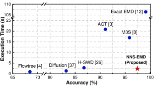
Figure 1: Execution time versus classification accuracy among exact EMD and SOTA approximate EMD algorithms for the MNIST dataset [19].

A variety of approximate algorithms for EMD have been proposed to address the high computational overhead of computing the exact EMD [4, 18, 37, 17, 26, 27, 3, 16]. Some algorithms employ pre-defined data structures (e.g., trees or graphs) to store entire datasets offline[4, 18, 37, 17]. Leveraging auxiliary data structures, these algorithms can achieve linear time complexity at the expense of additional memory space and lower accuracy. Other types of EMD approximations use entropic regularization [10, 1, 8], dimensional reduction [6, 27, 26], or constraints relaxation for OT [3, 16] to reduce the computation overhead, but also suffer various degrees of accuracy loss. Additionally, the performance of these approximation methods depends on parameter tuning.

In this paper, we propose NNS-EMD, a new approximate EMD algorithm that leverages nearest neighbor search (NNS). NNS-EMD achieves both high accuracy and relatively low execution time compared to the exact EMD and the existing state-of-the-art (SOTA) approximate EMD algorithms, as shown in Fig. 1. Instead of evaluating all possible point-to-point distances as in the exact EMD calculation, our proposed NNS-EMD focuses on identifying the nearest neighbors (NNs). This approach significantly reduces the number of data points to be compared and usually does not involve a linear number of iterations in experiments. Note that neighbor distances not only have been theoretically proven as close approximations of the global distance between two images [7], but are also extensively employed in the 3D point cloud domain [43, 27, 22]. Our main contributions are as follows:

• We propose an efficient EMD approximation, NNS-EMD, based on nearest neighbor search, which can achieve both high accuracy and low execution time.

• We provide theoretical analysis for the time complexity and error bound of the proposed NNS-EMD.

• We introduce a highly parallel implementation using GPU vectorization to further accelerate NNS-EMD.

We comprehensively evaluate NNS-EMD for image classification and retrieval tasks, and compare it with the exact EMD and other SOTA approximate EMD algorithms in terms of accuracy, execution time, and memory usage. NNS-EMD also generates transport mapping and accomplishes color transfer across images. These tasks are widely used to evaluate the performance of approximate EMD algorithms [4, 26, 8]. Our experimental results indicate that NNS-EMD significantly outperforms the exact EMD implementation, achieving 44$\times$ to 135$\times$ speedup, and also obtains up to 5% higher accuracy compared to the other SOTA EMD approximations.

2 Background

This section reviews the definition and mathematical formulation of EMD and then discusses SOTA algorithms for approximating EMD.

2.1 EMD and Optimal Transport

EMD is a mathematical metric for measuring the similarity between two probability distributions. It can be intuitively interpreted as the minimum total cost for transforming one probability distribution to another. We focus on the case where the two probability distributions are discrete. Let $S$ and $C$ denote two discrete probability distributions on a finite metric space $\mathcal{M}=(X,d_{X})$ ($S$ stands for “suppliers” and $C$ stands for “consumers”). $S$ and $C$ can be formulated as two histograms, where $s_{i}$ is the weight of the $i$-th bin of $S$ and $c_{j}$ is the weight of the $j$-th bin of $C$. Suppose $S$ and $C$ have $m$ and $n$ bins with positive weights and both distributions are normalized (i.e., $\sum_{i}s_{i}=\sum_{j}c_{j}=1$). The EMD between $S$ and $C$ is defined as:

$$\mbox{EMD}(S,C) =\min_{F_{i,j}\geq 0}\textstyle\sum_{i,j}F_{i,j}D_{i,j}$$ (1)

subject to: $$\textstyle\sum_{i}F_{i,j}=c_{j},$$ (2)

$$\textstyle\sum_{j}F_{i,j}=s_{i},$$ (3)

where $\mathbf{D}$ is a known $m\times n$ non-negative symmetric distance matrix, and $\mathbf{F}$ is a non-negative $m\times n$ flow matrix to be optimized (each entry $F_{i,j}$ in $\mathbf{F}$ represents the amount of weight that flows from the $i$-th bin of $S$ to the $j$-th bin of $C$ in the transformation). The solution for $\mathbf{F}$ is optimized for the minimum total cost of transforming $S$ to $C$.

In the context of measuring similarity between images, image pixels can be formulated as bins in the histograms on which EMD is calculated. Each bin in a histogram is associated with a weight (e.g., $s_{i}$ or $c_{j}$) and a pixel coordinate based on which $\mathbf{D}$ can be calculated. $L_{1}$ and $L_{2}$ distances are popular choices for $D_{i,j}$ in the image domain.

There are two common types of histogram formulation for images: the first is spatial location-based histogram [4, 3, 10, 8], and the second is color intensity-based histogram [34, 8]. In the former, every pixel represents one histogram bin, its weight is given by the normalized pixel value, and its coordinate is based on the pixel position. In the latter formulation, the number of bins is determined by the number of distinct pixel values, and the weight of a bin is the normalized frequency of its pixel value and its coordinate is represented by the RGB values of the pixel.

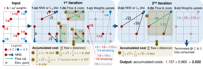
Figure 2: A toy example illustrating the pipeline of NNS-EMD. The inputs are $C$ and $S$, two sets of data points with weights and position coordinates (e.g., pixels in two images). “w/ ” denotes “with” . In steps 1-(a) and 2-(a), NNS-EMD identifies the nearest neighbor (NN) in $S$ for each point in $C$ to form groups based on the $L_{2}$ distance. Steps 1-(b) and 2-(b) compute flows between the NN pairs in $S$ and $C$ and calculate the cost for each group. Steps 1-(c) and 2-(c) update the weight for each data point and eliminate the points with zero weight.

2.2 Related Work

In the realm of EMD approximations, various innovative methods have been proposed. The Flowtree method [4] embeds a dataset into a tree structure to facilitate the matching of queries in a hierarchical manner. The Diffusion method [37] diffuses distributions across multi-scale graphs, comparing diffused histograms to approximate EMD. The hierarchical sliced Wasserstein distance (H-SWD) method [26] implements a hierarchical scheme for projecting datasets into one-dimensional distributions, enhancing efficiency for high-dimensional data. The Approximate Iterative Constrained Transfers (ACT) method [3] improves R-WMD [16] by imposing relaxed constraint (2) through iterations. Finally, the Multi-scale Sparse Sinkhorn (M3S) method [8] partitions a dataset hierarchically into subsets, integrating a multi-scale approach with the Sinkhorn algorithm for EMD approximation.

3 Methodology

In this section, we present our NNS-EMD algorithm and discuss key insights and challenges for each stage. We also perform a comprehensive theoretical analysis of the error bounds of the NNS-EMD solution and time complexity. Lastly, we conduct an in-depth examination of NNS-EMD and further accelerate it by leveraging GPU parallelism.

3.1 NNS-EMD Algorithm

The inputs to NNS-EMD are two sets $S$ and $C$ of data points (e.g., pixels in images) with coordinates and normalized weights, and the output is an approximate EMD (i.e., the total cost for transforming $S$ to $C$). The iterative algorithm consists of 3 key steps: NNS operation, flow & cost calculation, and weight update. A schematic diagram of the algorithm is given in Fig. 2 (for demonstration purposes, it only displays the first two iterations). The algorithm keeps running until convergence, which is defined as: the weight of every data point in $S$ is completely consumed and becomes zero. The location-based histogram described in Sec. 2.1 is employed, and the NNS is based on the $L_{2}$ distance between two position coordinates from $S$ and $C$.

Alg. 1 shows the full details of NNS-EMD. Below, we explain each of its three key steps and their motivations.

NNS Operation. The NNS operation identifies the supplier in $S$ that is the closest to every consumer point from $C$ according to the $L_{2}$ distance (Fig. 2 1-(a) and 2-(a)). There are two advantages of using NNS: (i) Compared to known data structure-based methods (e.g., tree and graph structures), NNS provides a more direct spatial proximity between two points and can better preserve local structures because no embedding of the original data points into a data structure is needed. (ii) Compared to the LP-based exact EMD computation, NNS-EMD can reduce time complexity by calculating transportation costs only between the nearest neighbor pairs instead of evaluating all possible pairs of points. Furthermore, we analyze the NNS operation and develop a near-linear time GPU implementation in Sec. 3.4. This implementation avoids the quadratic time complexity associated with repeated distance evaluations between every pair of data points in $S$ and $C$, thereby enhancing computational efficiency. Note that the choice of distance metric is pivotal for the NNS operation. We examine both the $L_{1}$ and $L_{2}$ distances in the experiments (Sec. 4.7), and $L_{2}$ distance-based implementation achieves superior accuracy and robustness. Thus, we adopt the $L_{2}$ distance in the rest of the paper as supported by experimental results.

Flow & Cost Calculation. In each iteration, after pairing every point in $C$ with its NN in $S$, the algorithm calculates the flow and transportation cost (Fig. 2 1-(b) and 2-(b)). If the $i$-th supplier from $S$ is matched with only the $j$-th consumer in $C$ as its NN, flow $F_{i,j}$ from the former to the latter is defined as $\min\{s_{i},c_{j}\}$. Note that $s_{i}$ and $c_{j}$ are the current weight stored in $i$-th supplier and the $j$-th consumer respectively, as they both need to be updated in the next step for every iteration.

Next, we will discuss how a supplier assigns its weight when is connected by multiple consumers. When multiple consumers share the same NN (e.g., the $i$-th supplier from $S$ is identified as the NN by both the $j_{1},j_{2}$-th consumers from $C$), and if $s_{i}\geq c_{j_{1}}+c_{j_{2}}$ (i.e., the weight $s_{i}$ stored in the $i$-th supplier can meet the demands of all these consumers), we allocate $s_{i}$ to each consumer, possibly with some remaining weight after this allocation. When $s_{i}$ is smaller than the sum of the weights stored in these consumers (the supplier cannot meet all the demands), we need to design a protocol to “optimally” allocate the “limited” $s_{i}$.

One intuitive scheme, named Random Protocol (RP), is to randomly assign $s_{i}$ to these consumers until $s_{i}$ is depleted. Alternatively, we may use a Greedy Protocol (GP) that assigns priorities to the matched consumers based on the distance matrix $\mathbf{D}$, with a closer consumer having a higher priority to receive from supplier $i$. For example, if $D_{i,j_{1}}\leq D_{i,j_{2}}$, we first calculate $F_{i,j_{1}}=\min\{s_{i},c_{j_{1}}\}$ and update $s_{i}$ before calculating $F_{i,j_{2}}$. The GP could be more time-consuming than the RP as it involves an additional step of ranking the distances of the consumers that are paired with the $i$-th supplier. Yet, the GP is more conceptually consistent with the exact EMD and is expected to yield a more accurate EMD approximation. We implement both the protocols in our experiments, and the results suggest that the GP gives higher accuracy at the expense of increased execution time (see discussions below).

After the flow values $F_{i,j}$ are determined, the algorithm computes the transportation cost for each flow, i.e., $F_{i,j}\times D_{i,j}$, where $D_{i,j}$ is an entry in the distance matrix $\mathbf{D}$. The total transportation cost in an iteration is $\sum_{i,j}(F_{i,j}\times D_{i,j})$.

Weights Update. In this step, the weights of all the points in both $S$ and $C$ that are involved in the NNS and the flow calculation steps are updated (Fig. 2 1-(c) and 2-(c)). Specifically, $s_{i}\leftarrow\min\{0,s_{i}-\sum_{j}F_{i,j}\}$ and $c_{j}\leftarrow\min\{0,c_{j}-F_{i,j}\}$, provided that one supplier may have multiple consumers whereas each consumer has only one supplier. When a point’s weight is fully exhausted or consumed, it is eliminated, and only the points with positive weights will participate in the next iteration. The weight update operation not only ensures the convergence of the NNS-EMD algorithm until all the points are consumed, but also contributes to efficient computation with a continuously reduced set of data points entering subsequent iterations of the algorithm.

Algorithm 1 NNS-EMD $(S,C,\mathbf{D})$

1:Input: Histograms $S$ and $C$, and distance matrix $\mathbf{D}$

2:$R=0$ $\triangleright$ initialize accumulated cost $R$

3:$\mathbf{F}^{*}\!\!=[0]_{m\times n}$ $\triangleright$ initialize the flow matrix $\mathbf{F}^{*}$

4:$t=1$ $\triangleright$ initialize the index of NNS iteration $t$

5:while $\exists c_{j}>0$ do$\triangleright$ while there is weight in $c_{j}$

6:     $\mathbf{m}^{(t)}\!=\{i\ |\ s_{i}>0\}$$\triangleright$ update indices for $S$

7:     $\mathbf{n}^{(t)}\!=\{j\ |\ c_{j}>0\}$$\triangleright$ update indices for $C$

8:     for $j\in\mathbf{n}^{(t)}$ do $\triangleright$ iterate for every active $j$ in $C$

9:         $\mbox{NNS}(j)\!\!=\!\mbox{argmin}_{i\in\mathbf{m}^{(t)}}\!\{D_{i,j}\}$ $\triangleright$ NNS in $S$

10:     end for

11:     for $i\in\mathbf{m}^{(t)}$ do$\triangleright$ iterate for every active $i$ in $S$

12:         $\mathbf{a}_{i}^{(t)}\!\!=\!\{j\ |\ c_{j}>0,\mbox{NNS}(j)\!=\!i\}$

13:         $\widetilde{\mathbf{a}}_{i}^{(t)}\!\!\!=\!\mbox{argsort}(D_{i,\mathbf{a}_{i}^{(t)}}\!)$ $\triangleright$ sort indices by dist. val.

14:         $l=1$ $\triangleright$ initialize $l$

15:         while $s_{i}>0$ and $l<|\widetilde{\mathbf{a}}^{(t)}_{i}|$ do

16:              $f=\min(s_{i},c_{\widetilde{\mathbf{a}}^{(t)}_{i}[l]})$ $\triangleright$ max weight to flow

17:              $s_{i}=s_{i}-f$ $\triangleright$ update weight of $s_{i}$

18:              $c_{\widetilde{\mathbf{a}}^{(t)}_{i}[l]}\!\!=\!c_{\widetilde{\mathbf{a}}^{(t)}_{i}[l]}\!\!-\!f$ $\triangleright$ update weight of $c_{\widetilde{\mathbf{a}}^{(t)}_{i}[l]}$

19:              $R=R+f\cdot D_{i,\widetilde{\mathbf{a}}^{(t)}_{i}[l]}$ $\triangleright$ accumulate cost

20:              $F^{*}_{i,\widetilde{\mathbf{a}}^{(t)}_{i}[l]}=F^{*}_{i,\widetilde{\mathbf{a}}^{(t)}_{i}[l]}+f$ $\triangleright$ update $\mathbf{F}^{*}$

21:              $l=l+1$ $\triangleright$ increase $l$

22:         end while

23:     end for

24:     $t=t+1$ $\triangleright$ increase $t$

25:end while

26:Output: $R$, $\mathbf{F}^{*}$

3.2 Error Analysis

We provide theoretical analysis of the error bounds between our NNS-EMD solution (output $R$) by Alg. 1 and the exact EMD. The proofs are given in the supplementary material.

First, we list the notation used in the theoretical analysis. In the $t$-th iteration of Alg. 1, $\mathbf{n}^{(t)}$ contains the indices of the positive bins in $C$, $\mathbf{m}^{(t)}$ contains the indices of the positive bins in $S$, $\mathbf{a}_{i}^{(t)}$ denotes the indices of the bins in $C$ that identify the $i$-th supplier from $S$ as NN, and $\widetilde{\mathbf{a}}_{i}^{(t)}\!\!=\!\mbox{argsort}(D_{i,\mathbf{a}^{(t)}_{i}})$ is the sorted version of $\mathbf{a}_{i}^{(t)}$ according to the distance to the $i$-th supplier.

Lemma 1 ($\mathbf{F}^{*}$ is a feasible solution).

Assume for an $i\in\{1,2,\ldots,m\}$, the $i$-th supplier from $S$ has at least one matched consumer for $\Delta$ iterations for an integer $\Delta>0$. Without loss of generality, assume $i\in\mathbf{m}^{(t_{1})}\cap\mathbf{m}^{(t_{2})}\cap\cdots\cap\mathbf{m}^{(t_{\Delta})}$ with $t_{1}<t_{2}<\cdots<t_{\Delta}$, and for $u\in\{t_{1},t_{2},\ldots,t_{\Delta}\},|\mathbf{a}_{i}^{(u)}|\geq 1$ (in other words, the $i$-th supplier is first identified in the $t_{1}$-th iteration as an NN to some point in $C$ and its weight is not exhausted until the $t_{\Delta}$-th iteration). Then,

$$\textstyle\sum_{u=t_{1}}^{t_{\Delta}}\sum_{l=1}^{|\mathbf{a}^{(u)}_{i}|}F^{*}_{i,\widetilde{\mathbf{a}}^{(u)}_{i}[l]}=s_{i},$$ (4)

implying that $F^{*}$ is a feasible solution to (1) satisfying constraints (2) and (3) in Section 2.1.

Based on Lemma 1, we upper-bound the total transport cost difference between $\mathbf{F}^{*}$ (computed by Alg. 1) and any feasible flows $\mathbf{F}$, and the difference between the EMD solution $R$ from Alg. 1 and the exact EMD in Theorem 1. Furthermore, with an additional assumption, we can further establish the exactness of $R$ as an approximation to the exact EMD in Theorem 2.

Theorem 1 (Error bound of EMD approximation by NNS-EMD).

Let $\mathbf{F}$ be any feasible flows, and $\mathbf{F}^{opt}$ be the optimal flow solution to (1) satisfying constraints (2) and (3) in Section 2.1. For the $i$-th supplier from $S$ defined in Lemma 1, let $j^{*}_{i}=\widetilde{\mathbf{a}}^{(t_{\Delta})}_{i}[k^{(t_{\Delta})}_{i}]$ be the index of the last consumer from $C$ that receives a positive flow from $s_{i}$ before $s_{i}$ is eliminated, with $1\leq k^{(t_{\Delta})}_{i}\leq|\mathbf{a}^{(t_{\Delta})}_{i}|$. Then,

$$\textstyle\sum_{j}F^{*}_{i,j}D_{i,j}-\sum_{j}F_{i,j}D_{i,j}\leq\>D_{i,j^{*}_{i}},$$ (5)

and the difference between $R$ (the approximate EMD from Alg. 1) and the optimal EMD is:

$$\textstyle 0\leq\sum_{i,j}F^{*}_{i,j}D_{i,j}-\sum_{i,j}F^{opt}_{i,j}D_{i,j}\leq\sum_{i}D_{i,j^{*}_{i}}.$$ (6)

Theorem 1 suggests that the difference between the approximate EMD from NNS-EMD and the optimal EMD is not greater than the cumulative distance from each supplier $s_{i}$ to the last consumer in $C$ to whom $s_{i}$ supplies a positive flow immediately before the elimination of $s_{i}$.

If we further assume that for each supplier $s_{i}$ from $S$, every consumer involved in eliminating $s_{i}$ has not received any weight from any suppliers until the iteration where $s_{i}$ is eliminated, we may claim the exactness of the approximation by Alg. 1 toward the optimal EMD in Theorem 2.

Theorem 2 (Exactness of EMD approximation by NNS-EMD).

Let $M_{\widetilde{\mathbf{a}}^{(u)}_{i}[l]}$ denote the accumulated consumed weight in the ${\widetilde{\mathbf{a}}^{(u)}_{i}[l]}$-th bin in $C$ immediately before the $u$-th iteration. Then for the $i$-th supplier from $S$ in Lemma 1, $\forall u\!\!\!\in\!\{t_{1},t_{2},\ldots,t_{\Delta-1}\}$ and $\forall l\!\!\in\{1,2,\ldots,|\widetilde{\mathbf{a}}^{(u)}_{i}|\}$,

$$F^{*}_{i,\widetilde{\mathbf{a}}^{(u)}_{i}[l]}=c_{\widetilde{\mathbf{a}}^{(u)}_{i}[l]}-M_{\widetilde{\mathbf{a}}^{(u)}_{i}[l]}.$$ (7)

If we assume $M_{\widetilde{\mathbf{a}}^{(u)}_{i}[l]}\!\!=0$ holds, we have $F^{*}_{i,\widetilde{\mathbf{a}}^{(u)}_{i}[l]}\!=c_{\widetilde{\mathbf{a}}^{(u)}_{i}[l]}$, and then for any feasible flows $\mathbf{F}$,

$$\textstyle\sum_{i,j}F^{*}_{i,j}D_{i,j}\leq\sum_{i,j}F_{i,j}D_{i,j}.$$ (8)

Therefore, $R=\sum_{i,j}F^{opt}_{i,j}D_{i,j}$.

3.3 Time Complexity Analysis

Using the same notation, let the numbers of bins in $S$ and $C$ be $m$ and $n$, respectively. Then the size of the distance matrix $\mathbf{D}$ is $m\times n$. Without loss of generality, we assume $n\geq m$. Then for every iteration in Alg. 1, the time complexity for the step of NNS is $O(n^{2})$. Also, the sorting time complexity in Line 13 of Alg. 1 is $O(n\log n)$.

Let $T$ be the total number of NNS iterations for Alg. 1 to converge, and $\gamma_{t}=n_{t+1}/n_{t}$ be the ratio of consumer set sizes between two consecutive NNS iterations. Note that $\gamma_{t}\leq 1$ and $n_{1}=n$. Then:

$$\underbrace{n_{1}^{2}+n_{2}^{2}+n^{2}_{3}+\cdots+n_{T}^{2}}_{\text{NNS}}+\underbrace{n_{1}\log n_{1}+\cdots+n_{T}\log n_{T}}_{\text{Sorting}}$$

$$\leq \>(n_{1}^{2}+n_{2}^{2}+n^{2}_{3}+\cdots+n_{T}^{2})+(n_{1}^{2}+n_{2}^{2}+n_{3}^{2}+\cdots+n_{T}^{2})$$

$$= \>2(n^{2}+\gamma^{2}_{1}n^{2}+\gamma^{2}_{1}\gamma^{2}_{2}n^{2}+\cdots+\Pi_{t=1}^{T-1}\gamma^{2}_{t}n^{2})$$

$$= \>2n^{2}(1\!+\!\gamma^{2}_{1}+\gamma^{2}_{1}\gamma^{2}_{2}+\cdots+\Pi_{t=1}^{T-1}\gamma^{2}_{t})\!<\!2n^{2}(1+T)\!\!\!$$ (9)

To investigate the dominant term in Eq. (9), we conduct an experiment to explore the relationship between $T$ vs $n$ and $n/\log(n)$ across various image sizes using the NUS-WIDE [9] and DOTmark [35] datasets. To enhance the reliability of our findings, we repeat this experiment $300$ times and calculate the average $T$ and its range. The empirical results for the NUS-WIDE dataset are in Fig. 3, and the results for the DOTmark dataset can be found in the supplementary material. Both results suggest $T=o(n/\log(n))=o(n)$. Given that the relation is based on empirical results, we take the more conservative bound of $T=o(n)$, plug it in Eq. (9) and obtain Claim 1 below.

Claim 1.

In general, the time complexity of NNS-EMD is $O(n^{2}\cdot o(n))$, supported by strong empirical evidence.

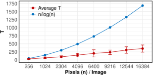
Figure 3: Relation between $T$ (average and range over 300 repeats) of NNS-EMD and image size $n$ (with $n/\log(n)$ as reference).

3.4 Accelerating NNS-EMD on GPU

We enhance NNS-EMD with both parallelized NNS operation and batch processing on GPU, leveraging parallelism at both the data point level and the dataset level.

Parallel NNS. Based on our theoretical analysis, the bottleneck of NNS-EMD is the NNS operation with a quadratic time complexity. As discussed in prior works [21, 29], the distance computations have no mutual dependencies. Therefore, we allocate the NNS operation for each consumer among $S$ to different GPU threads for parallel execution, which improves the execution time from quadratic to linear.

Batch Processing. To further improve the computational efficiency of NNS-EMD on large datasets, we utilize batch processing to reduce execution time. When computing NNS-EMD between $M$ supplier datasets and $N$ consumer datasets, we need to execute the algorithm $O(MN)$ times with a straightforward GPU implementation, which is inefficient for large datasets.

By parallelizing computations across batches, the execution times can be reduced to $O(Bb^{2})$, where $B$ is the number of batches and $b$ is the batch size (satisfying $bB=\max\{M,N\}$).

However, as discussed in Sec. 3.1, the zero-weight data points need to be eliminated in the weights update step, (Fig, 2 1-(c) and 2-(c)). Instead of removing the zero-weight data points from $\mathbf{D}$ directly, we assign penalty terms to these points, excluding them from the subsequent NNS iterations. This approach allows us to keep the size of $\mathbf{D}$ consistent across each iteration, facilitating data unrolling for nested loops via vectorization.

4 Experiments

We evaluate and benchmark NNS-EMD against an exact EMD algorithm as well as several SOTA approximate EMD methods on image classification and retrieval tasks. Evaluation metrics include accuracy, execution time, and memory usage. We also apply the proposed NNS-EMD to compute EMD between color images to achieve color transfer. Finally, we investigate the impact of batch processing on NNS-EMD’s performance and assess how different distance metrics ($L_{1}$ and $L_{2}$) affect accuracy.

Table 1: Description of the datasets used.

	# of Images	# of Queries	Image Size
MNIST	60,000	1,000	[28, 28]
CIFAR-10	50,000	1,000	[3, 32, 32]
NUS-WIDE	205,334	500	[3, 128, 128]
Paris-6k	6322	70	[3, 1024, 768]
DOTmark	500	500	[32, 32] to [512, 512]

4.1 Experimental Setup

Datasets. For image classification, we use the MNIST [19] and CIFAR-10 [14] datasets, following the works [37, 4, 13]. For image retrieval, we utilize the NUS-WIDE [9] and Paris-6k [28] datasets, as explored in [50, 45]. Additionally, the DOTmark [35] dataset is used for evaluating memory usage and analyzing the relative error between our proposed NNS-EMD and an exact EMD solution, as conducted in [8]. These datasets are summarized in Tab. 1. Detailed description of these datasets is presented in the supplementary material.

Additionally, for image pre-processing, we use the spatial location-based histogram to represent grayscale images (e.g., MNIST, DOTmark), and adopt the color intensity-based histogram for color images, as discussed in Sec. 2.1.

Algorithms & Implementations. We implement our NNS-EMD using both the greedy protocol (GP) and random protocol (RP) on a GPU with batch processing. For the NNS operation, we use $L_{2}$ distance for higher accuracy and robustness. We also compare $L_{1}$ and $L_{2}$ distances in Sec. 4.7. We implement the exact EMD [12] and various SOTA approximate EMD algorithms, including Flowtree [4], Diffusion EMD[37], ACT [3], M3S [8], and H-SWD [26]. The exact EMD, Flowtree, and Diffusion algorithms are implemented on CPU, and the other algorithms are implemented on GPU, which are consistent with their implementations in the respective original papers. Note that parallelizing the exact EMD, Flowtree, and Diffusion methods on GPU is challenging due to the data dependencies inherent in each iteration of these methods.

Metrics. For image classification, we adopt accuracy, precision, recall, and F1-score as performance metrics [38]. For image retrieval, we use two widely-adopted metrics [49]: recall and mean average precision (MAP). Execution time is measured by the average execution time for processing a single query. Detailed metric explanations are given in the supplementary material.

Table 2: Comparison between NNS-EMD (GP) and the exact EMD in terms of execution time and accuracy.

	Execution Time (s)			Accuracy
Dataset	Exact EMD	NNS-EMD	Speedup	Exact EMD	NNS-EMD
MNIST	106.47	2.39	44.55$\times$	99.12%	97.45%
CIFAR-10	1163.50	8.57	135.77$\times$	85.34%	82.12%

Table 3: Comparison of approximate EMD algorithms for image classification.

	MNIST					CIFAR-10
Algorithm	Accuracy	Precision	Recall	F1-score	Time (s)	Accuracy	Precision	Recall	F1-score	Time (s)
ACT	91.05%	0.9029	0.9009	0.9019	20.87	71.68%	0.7052	0.7014	0.7017	84.62
Flowtree	68.45%	0.6634	0.6658	0.6647	0.94	46.57%	0.4589	0.4501	0.4545	5.42
Diffusion	83.21%	0.8298	0.8301	0.8299	1.34	64.21%	0.6400	0.6392	0.6396	8.98
H-SWD	86.78%	0.8614	0.8621	0.8611	2.80	70.24%	0.6990	0.6986	0.6988	13.57
M3S	95.87%	0.9514	0.9475	0.9485	16.93	76.98%	0.7684	0.7602	0.7643	78.50
NNS-EMD (RP)	95.19 %	0.9502	0.9509	0.9500	1.57	76.42%	0.7589	0.7610	0.7600	6.13
NNS-EMD (GP)	97.45%	0.9741	0.9748	0.9720	2.39	82.12%	0.8161	0.8149	0.8155	8.57
RP: random protocol; GP: greedy protocol.

Table 4: EMD approximations on image retrieval.

	NUS-WIDE			Paris-6k
Algorithm	Recall	MAP	Time (min)	Recall	MAP	Time (s)
ACT	0.727	0.630	36.44	0.605	0.542	314.23
Flowtree	0.519	0.457	6.14	0.382	0.417	22.72
Diffusion	0.646	0.571	13.51	0.459	0.438	27.18
H-SWD	0.681	0.613	7.52	0.531	0.554	10.43
M3S	0.754	0.646	29.16	0.625	0.583	247.36
NNS-EMD (RP)	0.701	0.589	5.47	0.565	0.531	47.46
NNS-EMD (GP)	0.809	0.696	8.94	0.661	0.647	95.73

Platforms. We run the aforementioned CPU-based implementations on an Intel i9-12900K CPU with 128 GB of DDR4 memory, and the GPU-based implementations on an NVIDIA 3080Ti GPU with 12 GB of memory.

4.2 Image Classification

In the image classification task, we compare our NNS-EMD with both the exact EMD and approximate EMD algorithms. Tab. 2 shows the execution time and accuracy results of exact EMD and NNS-EMD. NNS-EMD achieves 44.55$\times$ and 135.77$\times$ speedup over an exact EMD realization on the MNIST and CIFAR-10 datasets, respectively, while incurring an accuracy loss of just 1.67% and 3.22%.

NNS-EMD is also benchmarked against SOTA approximate EMD algorithms. In Tab. 3, the experimental results show that our NNS-EMD is superior to all the other approximate EMD solutions in every metric except when compared to the execution time of the Flowtree and Diffusion method. Specifically, NNS-EMD with GP achieves $\sim$1.6% and $\sim$5% higher accuracy than the next-best algorithm (M3S) on MNIST and CIFAR-10, respectively. Additionally, NNS-EMD also achieves speedup of 7.08$\times$ and 9.16$\times$ over M3S on the two datasets respectively. Note that, although NNS-EMD with GP is 2.54$\times$ and 1.58$\times$ slower than the Flowtree solution, it is 29% and 36% more accurate than the Flowtree method on MNIST and CIFAR-10, respectively. Comparing the RP and GP protocol used in NNS-EMD, we observe that the GP improves the classification accuracy but comes at the cost of increased execution time, primarily due to the additional ranking operation.

4.3 Image Retrieval

We also conduct experiments on the image retrieval task using our NNS-EMD and benchmark it against other EMD approximations. To evaluate the scalability and adaptability of these algorithms, we deliberately choose two distinct datasets: the NUS-WIDE dataset [9] comprised of a large collection of images, and the Paris-6k dataset [28] consisting of a smaller set of high-resolution color images.

The experimental results are presented in Tab. 4. Observations indicate that NNS-EMD achieves the highest recall and MAP among all the compared approximate EMD methods. In the NUS-WIDE dataset, NNS-EMD with RP is even faster than the Flowtree method. This efficiency is attributed to NNS-EMD’s utilization of batch processing, particularly beneficial for large datasets like NUS-WIDE. For the Paris-6k dataset, although the H-SWD method is the fastest due to H-SWD’s ability to project high-resolution images into one-dimensional data, its recall and MAP are significantly less than NNS-EMD. Thus, NNS-EMD demonstrates remarkable scalability and performance in image retrieval tasks.

Additionally, we note that as image size increases, NNS-EMD with the RP achieves greater speedup than with the GP. Specifically, RP achieves $1.39\times$, $1.63\times$, and $2.02\times$ speedup compared to GP on the CIFAR-10, NUS-WIDE, and Paris-6k datasets, respectively. This is attributed to the fact that the additional ranking operation in GP becomes more time-consuming with larger image sizes.

4.4 Memory Usage Evaluation

In addition to the accuracy and performance metrics, we also evaluate the memory usage by NNS-EMD, the exact EMD solution, and the other SOTA approximate EMD algorithms. We conduct experiments on the DOTmark dataset following [8], and vary the image size from 32$\times$32 to 512$\times$512 (i.e., from 1024 to 262144 pixels). We employ the psutil library [31] to measure the memory usage of CPU-based implementations, and Nvidia-smi for GPU-based implementations.

As illustrated in Fig. 4, the NNS-EMD, M3S and ACT methods exhibit a linear growth in memory requirements, with NNS-EMD and ACT having similar slopes, while M3S shows a steeper slope. Flowtree approximation demonstrates a sub-linear increase in the memory usage. The H-SWD approximation shows constant or near-constant memory usage relative to the number of pixels, as its memory usage depends only on the number of projections. The diffusion and exact EMD approaches demonstrate a cubic increase in memory requirement, and exhaust available memory after image sizes of $256\times 256$ and $512\times 512$ pixels, respectively.

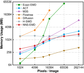
Figure 4: Memory usage of different algorithms.

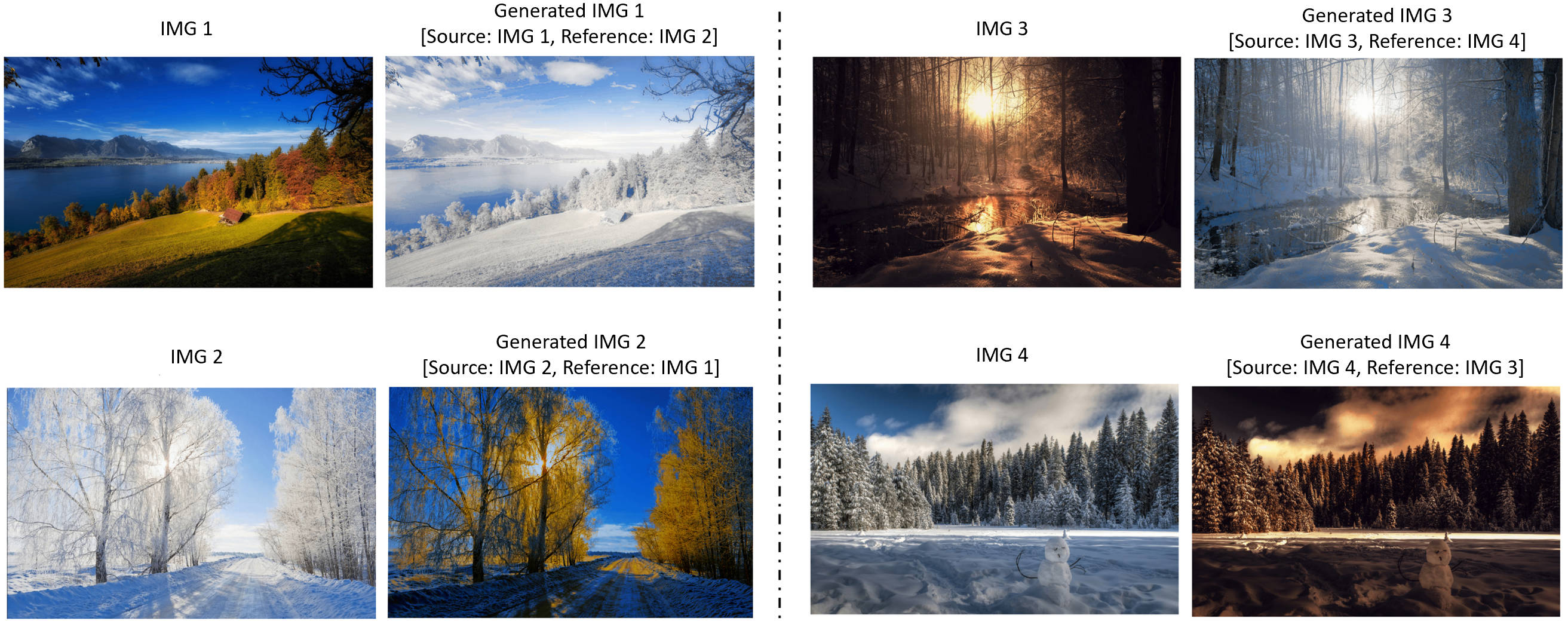
Figure 5: Color transfer applied to the original $1920\times 1200$ images IMGs. Each IMG serves both as the source and the reference. We determine the color transfer mapping from the source to the reference by NNS-EMD, resulting in the generated images.

4.5 Color Transfer between Images

Color transfer is gaining interest in computer vision and is widely applied in real-world applications, such as photo editing and underwater imaging [25, 30, 20, 46]. Color transfer aims to recolor a source image by deriving a mapping from one reference image (supplier) to this source image (consumer) [11].

Following the image pre-processing steps in [8, 5], we apply $k$-means clustering to reduce the image to $m$ distinct pixel vector in RGB space. By adopting the color intensity-based histogram formulation introduced in Sec. 2.1, there are $m$ bins for this color image. The weight of each bin is the normalized frequency of its pixel value and the coordinate is its corresponding RGB vector. After performing the same formulation for the source image with $n$ bins, NNS-EMD can be employed to output a transportation map $\mathbf{F}^{*}$.

We use $L_{2}$ distance and set $m=n=4096$ , following the setup in [5]. By adopting the transportation mapping from our NNS-EMD to replace the pixels in the source image, we showcase four color transfer examples across different seasons in Fig. 5. The generated images demonstrate high-quality color mappings between reference and source images, showing high fidelity, naturalness, and consistency.

4.6 Vectorization on GPU

To further accelerate NNS-EMD, we propose a data-parallel implementation leveraging vectorization on GPU. In this experiment, we evaluate the impact of vectorization on NNS-EMD’s execution time. Our experiments use the DOTmark dataset [35], with the number of images ranging from 1024 to 16364, to measure the execution time. As shown in Tab. 5, vectorization leads to a significant speedup compared to the non-vectorized implementation. Moreover, as the data size increases, the execution time of the vectorized implementations increase at a much slower rate than the non-vectorized implementations.

Table 5: Execution time (in seconds) of NNS-EMD with/without vectorization on different numbers of images in DOTmark.

	Execution Time (s)
No. of Images	1024	2048	4096	8192	16384
w/o Vectorization	52.29	137.80	278.44	558.01	1108.32
w/ Vectorization	20.92	27.25	32.64	40.05	48.19

Table 6: Mean and standard deviation of RE (%) between NNS-EMD and the exact EMD with either $L_{1}$ or $L_{2}$ distance on various sizes of images.

	Mean (Standard Deviation) of RE (%)
Pixels/Image	1024	4096	9216	16384
$L_{1}$	0.22 (0.14)	0.67 (0.31)	0.49 (0.24)	0.52 (0.37)
$L_{2}$	0.15 (0.07)	0.32 (0.11)	0.37 (0.08)	0.32 (0.09)

4.7 Comparison of $L_{1}$ and $L_{2}$ Distances

In NNS-EMD, the NNS operation needs a specific distance metric to measure the distances between data points, in order to identify nearest neighbors. This directly impacts the accuracy and robustness of the approximation results.

In Tab. 6, we compare the relative error and standard deviation of NNS-EMD with respect to the exact EMD to evaluate the $L_{1}$ and $L_{2}$ distance metrics on the DOTmark dataset. Relative Error (RE) is computed as $RE=|R_{p}-R_{p}^{opt}|/R_{p}^{opt}$, where $R_{p}$ and $R_{p}^{opt}$ represent the results computed by NNS-EMD and the exact EMD with $L_{p}$ distance ($p\in\{1,2\}$), respectively. To ensure the reliability of our findings, we repeat this experiment ten times by randomly picking images of each image size, and compute the mean and standard deviation of RE. Tab. 6 shows that the $L_{2}$-based NNS-EMD yields a more accurate approximation to the exact EMD than the $L_{1}$ distance. Further, the $L_{2}$ distance demonstrates superior stability over the $L_{1}$ distance.

5 Conclusions

In this work, we introduced NNS-EMD, a new computationally efficient EMD approximation method that relies on nearest neighbor search. Empirical evaluations confirm that NNS-EMD attains high accuracy with reduced execution time compared to SOTA approximate EMD algorithms. We also presented theoretical analysis on the time complexity and error bounds of NNS-EMD. We further accelerated NNS-EMD through exploiting GPU parallelism. As future work, we plan to investigate the integration of NNS-EMD as a loss function within deep learning frameworks, particularly for 3D point cloud applications.

References

- [1] Mokhtar Z Alaya, Maxime Berar, Gilles Gasso, and Alain Rakotomamonjy. Screening Sinkhorn algorithm for regularized optimal transport. Advances in Neural Information Processing Systems, 32, 2019.
- [2] Martin Arjovsky, Soumith Chintala, and Léon Bottou. Wasserstein generative adversarial networks. In Proceedings of the 34th International Conference on Machine Learning - Volume 70, ICML’17, page 214–223. JMLR.org, 2017.
- [3] Kubilay Atasu and Thomas Mittelholzer. Linear-complexity data-parallel earth mover’s distance approximations. In International Conference on Machine Learning, pages 364–373. PMLR, 2019.
- [4] Arturs Backurs, Yihe Dong, Piotr Indyk, Ilya Razenshteyn, and Tal Wagner. Scalable nearest neighbor search for optimal transport. In Hal Daumé III and Aarti Singh, editors, Proceedings of the 37th International Conference on Machine Learning, volume 119 of Proceedings of Machine Learning Research, pages 497–506. PMLR, 13–18 Jul 2020.
- [5] Mathieu Blondel, Vivien Seguy, and Antoine Rolet. Smooth and sparse optimal transport. In International Conference on Artificial Intelligence and Statistics, pages 880–889. PMLR, 2018.
- [6] Nicolas Bonneel, Julien Rabin, Gabriel Peyré, and Hanspeter Pfister. Sliced and radon Wasserstein barycenters of measures. Journal of Mathematical Imaging and Vision, 51:22–45, 2015.
- [7] Gunilla Borgefors. Distance transformations in arbitrary dimensions. Computer Vision, Graphics, and Image Processing, 27(3):321–345, 1984.
- [8] Yidong Chen, Chen Li, and Zhonghua Lu. Computing Wasserstein-p distance between images with linear cost. In Proceedings of the IEEE/CVF Conference on Computer Vision and Pattern Recognition, pages 519–528, 2022.
- [9] Tat-Seng Chua, Jinhui Tang, Richang Hong, Haojie Li, Zhiping Luo, and Yantao Zheng. NUS-WIDE: A real-world web image database from National University of Singapore. In Proceedings of the ACM International Conference on Image and Video Retrieval, pages 1–9, 2009.
- [10] Marco Cuturi. Sinkhorn distances: Lightspeed computation of optimal transport. Advances in Neural Information Processing Systems, 26, 2013.
- [11] H Sheikh Faridul, Tania Pouli, Christel Chamaret, Jürgen Stauder, Erik Reinhard, Dmitry Kuzovkin, and Alain Trémeau. Colour mapping: A review of recent methods, extensions and applications. In Computer Graphics Forum, volume 35, pages 59–88. Wiley Online Library, 2016.
- [12] Rémi Flamary, Nicolas Courty, Alexandre Gramfort, Mokhtar Z Alaya, Aurélie Boisbunon, Stanislas Chambon, Laetitia Chapel, Adrien Corenflos, Kilian Fatras, Nemo Fournier, et al. POT: Python optimal transport. The Journal of Machine Learning Research, 22(1):3571–3578, 2021.
- [13] Kaiming He, Xiangyu Zhang, Shaoqing Ren, and Jian Sun. Deep residual learning for image recognition. In Proceedings of the IEEE Conference on Computer Vision and Pattern Recognition, pages 770–778, 2016.
- [14] Alex Krizhevsky, Geoffrey Hinton, et al. Learning multiple layers of features from tiny images. 2009.
- [15] Harold W Kuhn. The Hungarian method for the assignment problem. Naval Research Logistics Quarterly, 2(1-2):83–97, 1955.
- [16] Matt Kusner, Yu Sun, Nicholas Kolkin, and Kilian Weinberger. From word embeddings to document distances. In International Conference on Machine Learning, pages 957–966. PMLR, 2015.
- [17] Tam Le, Truyen Nguyen, Dinh Phung, and Viet Anh Nguyen. Sobolev transport: A scalable metric for probability measures with graph metrics. In International Conference on Artificial Intelligence and Statistics, pages 9844–9868. PMLR, 2022.
- [18] Tam Le, Makoto Yamada, Kenji Fukumizu, and Marco Cuturi. Tree-sliced variants of Wasserstein distances. Advances in Neural Information Processing Systems, 32, 2019.
- [19] Yann LeCun, Léon Bottou, Yoshua Bengio, and Patrick Haffner. Gradient-based learning applied to document recognition. Proceedings of the IEEE, 86(11):2278–2324, 1998.
- [20] Chongyi Li, Jichang Guo, and Chunle Guo. Emerging from water: Underwater image color correction based on weakly supervised color transfer. IEEE Signal processing letters, 25(3):323–327, 2018.
- [21] Shengren Li and Nina Amenta. Brute-force k-nearest neighbors search on the GPU. In Similarity Search and Applications: 8th International Conference, Proceedings 8, pages 259–270. Springer, 2015.
- [22] Fangzhou Lin, Yun Yue, Songlin Hou, Xuechu Yu, Yajun Xu, Kazunori D Yamada, and Ziming Zhang. Hyperbolic Chamfer distance for point cloud completion. In Proceedings of the IEEE/CVF International Conference on Computer Vision, pages 14595–14606, 2023.
- [23] Haibin Ling and Kazunori Okada. An efficient earth mover’s distance algorithm for robust histogram comparison. IEEE Transactions on Pattern Analysis and Machine Intelligence, 29(5):840–853, 2007.
- [24] Minghua Liu, Lu Sheng, Sheng Yang, Jing Shao, and Shi-Min Hu. Morphing and sampling network for dense point cloud completion. In Proceedings of the AAAI Conference on Artificial Intelligence, volume 34, pages 11596–11603, 2020.
- [25] Shiguang Liu. An overview of color transfer and style transfer for images and videos. arXiv preprint arXiv:2204.13339, 2022.
- [26] Khai Nguyen, Tongzheng Ren, Huy Nguyen, Litu Rout, Tan Nguyen, and Nhat Ho. Hierarchical sliced Wasserstein distance. International Conference on Learning Representations, 2023.
- [27] Trung Nguyen, Quang-Hieu Pham, Tam Le, Tung Pham, Nhat Ho, and Binh-Son Hua. Point-set distances for learning representations of 3D point clouds. In Proceedings of the IEEE/CVF International Conference on Computer Vision, pages 10478–10487, 2021.
- [28] James Philbin, Ondrej Chum, Michael Isard, Josef Sivic, and Andrew Zisserman. Lost in quantization: Improving particular object retrieval in large scale image databases. In 2008 IEEE Conference on Computer Vision and Pattern Recognition, pages 1–8. IEEE, 2008.
- [29] Nikhila Ravi, Jeremy Reizenstein, David Novotny, Taylor Gordon, Wan-Yen Lo, Justin Johnson, and Georgia Gkioxari. Accelerating 3D deep learning with PyTorch3D. arXiv:2007.08501, 2020.
- [30] Erik Reinhard, Michael Adhikhmin, Bruce Gooch, and Peter Shirley. Color transfer between images. IEEE Computer graphics and applications, 21(5):34–41, 2001.
- [31] Giampaolo Rodola. psutil: Cross-platform library for retrieving information on running processes and system utilization, 2021.
- [32] Litu Rout, Alexander Korotin, and Evgeny Burnaev. Generative modeling with optimal transport maps. In International Conference on Learning Representations, 2021.
- [33] Yossi Rubner, Carlo Tomasi, and Leonidas J Guibas. A metric for distributions with applications to image databases. In Sixth International Conference on Computer Vision (IEEE Cat. No. 98CH36271), pages 59–66. IEEE, 1998.
- [34] Yossi Rubner, Carlo Tomasi, and Leonidas J Guibas. The earth mover’s distance as a metric for image retrieval. International Journal of Computer Vision, 40:99–121, 2000.
- [35] Jörn Schrieber, Dominic Schuhmacher, and Carsten Gottschlich. DOTmark – a benchmark for discrete optimal transport. IEEE Access, 5:271–282, 2016.
- [36] Sameer Shirdhonkar and David W Jacobs. Approximate earth mover’s distance in linear time. In 2008 IEEE Conference on Computer Vision and Pattern Recognition, pages 1–8. IEEE, 2008.
- [37] Alexander Y Tong, Guillaume Huguet, Amine Natik, Kincaid MacDonald, Manik Kuchroo, Ronald Coifman, Guy Wolf, and Smita Krishnaswamy. Diffusion earth mover’s distance and distribution embeddings. In International Conference on Machine Learning, pages 10336–10346. PMLR, 2021.
- [38] Milan Tripathi. Analysis of convolutional neural network based image classification techniques. Journal of Innovative Image Processing (JIIP), 3(02):100–117, 2021.
- [39] Dahlia Urbach, Yizhak Ben-Shabat, and Michael Lindenbaum. DPDist: Comparing point clouds using deep point cloud distance. In Computer Vision–ECCV 2020: 16th European Conference, Part XI 16, pages 545–560. Springer, 2020.
- [40] Cédric Villani et al. Optimal Transport: Old and New, volume 338. Springer, 2009.
- [41] Gary R Waissi. Network flows: Theory, algorithms, and applications, 1994.
- [42] Lingfei Wu, Ian En-Hsu Yen, Kun Xu, Fangli Xu, Avinash Balakrishnan, Pin-Yu Chen, Pradeep Ravikumar, and Michael J. Witbrock. Word mover’s embedding: From Word2Vec to document embedding. In Ellen Riloff, David Chiang, Julia Hockenmaier, and Jun’ichi Tsujii, editors, Proceedings of the 2018 Conference on Empirical Methods in Natural Language Processing, pages 4524–4534, Brussels, Belgium, Oct.-Nov. 2018. Association for Computational Linguistics.
- [43] Tong Wu, Liang Pan, Junzhe Zhang, Tai Wang, Ziwei Liu, and Dahua Lin. Density-aware Chamfer distance as a comprehensive metric for point cloud completion. arXiv preprint arXiv:2111.12702, 2021.
- [44] Liang Xie, Jialie Shen, Jungong Han, Lei Zhu, and Ling Shao. Dynamic multi-view hashing for online image retrieval. IJCAI, 2017.
- [45] Jian Xu, Chunheng Wang, Chengzuo Qi, Cunzhao Shi, and Baihua Xiao. Iterative manifold embedding layer learned by incomplete data for large-scale image retrieval. IEEE Transactions on Multimedia, 21(6):1551–1562, 2018.
- [46] Hua Yang, Fei Tian, Qi Qi, QM Jonathan Wu, and Kunqian Li. Underwater image enhancement with latent consistency learning-based color transfer. IET Image Processing, 16(6):1594–1612, 2022.
- [47] Gang Yao and Ashwin Dani. Visual tracking using sparse coding and earth mover’s distance. Frontiers in Robotics and AI, 5:95, 2018.
- [48] Chen Zhao, Chun Fai Lui, Shichang Du, Di Wang, and Yiping Shao. An earth mover’s distance based multivariate generalized likelihood ratio control chart for effective monitoring of 3D point cloud surface. Computers & Industrial Engineering, 175:108911, 2023.
- [49] Liang Zheng, Liyue Shen, Lu Tian, Shengjin Wang, Jingdong Wang, and Qi Tian. Scalable person re-identification: A benchmark. In Proceedings of the IEEE International Conference on Computer Vision, pages 1116–1124, 2015.
- [50] Han Zhu, Mingsheng Long, Jianmin Wang, and Yue Cao. Deep hashing network for efficient similarity retrieval. In Proceedings of the AAAI Conference on Artificial Intelligence, volume 30, 2016.