Spatial distribution of ultracold neutron probability density
in the gravitational field of the earth above a mirror
Abstract
We propose a theoretical analysis of the experimental data by Ichikawa et al. (Phys. Rev. Lett. 112, 071101 (2014)) on a spatial distribution of ultracold neutrons in the gravitational field of the Earth above a mirror, projected onto a pixelated detector by scattering by a cylindrical mirror. We calculate a theoretical spatial distribution of a probability density of quantum gravitational states of ultracold neutrons and analyse a spatial distribution of quantum gravitational states in term of the Wigner function. We cannot confirm that the experimental data by Ichikawa et al. (Phys. Rev. Lett. 112, 071101 (2014)) correspond to a spatial distribution of quantum gravitational states of ultracold neutrons.
pacs:
03.65.Ge, 13.15.+g, 23.40.Bw, 26.65.+tI Introduction
Quantum gravitational states of ultracold neutrons in the gravitational field of the Earth above a mirror Gibbs1975 have been observed experimentally in Nesvizhevsky2002 –Abele2010 . The experimental analysis of a spatial distribution of a probability density of quantum gravitational states of ultracold neutrons has been carried out in AbeleWF1 ; AbeleWF2 by measuring of a free fall of ultracold neutrons on a mirror and reviewed in AbeleWF3 . In turn, the measurements of transitions between quantum gravitational states of ultracold neutrons, bouncing between two mirrors in the gravitational field of the Earth, have been performed in Jenke2011 ; Jenke2012 . The wave functions and the binding energies of quantum gravitational states of ultracold neutrons, located between two mirrors, have been calculated in Ivanov2013 . Recently the experimental data on a spatial distribution of the ultracold neutrons in the gravitational field of the Earth above a mirror, obtained by Ichikawa et al. Ichikawa2014 , have been interpreted as a spatial distribution of the quantum gravitational states of ultracold neutrons. The authors have investigated a vertical distribution of ultracold neutrons, moved above a horizontal mirror and projected onto a pixelated horizontal detector above a mirror by scattering by a cylindrical mirror. An observed spatial modulation of a spatial distribution of ultracold neutrons has been interpreted as a spatial distribution of quantum gravitational states of ultracold neutrons. For a confirmation of such an interpretation the authors have carried out a theoretical analysis of the experimental data by using the Wigner function Wigner1932 .
In this paper we analyse a spatial distribution of quantum gravitational states of ultracold neutrons for the experimental setup by Ichikawa et al. Ichikawa2014 . A spatial distribution of quantum gravitational states of ultracold neutrons we analyse in terms of i) a spatial distribution of a probability density Davydov1965 and ii) a spatial distribution of the Wigner function Wigner1932 of quantum gravitational states of ultracold neutrons. Unfortunately our theoretical analysis cannot confirm that the experimental data by Ichikawa et al. Ichikawa2014 correspond to a spatial distribution of quantum gravitational states of ultracold neutrons.
II Experimental setup of Ichikawa’s experiment on spatial distribution of quantum gravitational states of ultracold neutrons
The experimental setup of the experiment on the measurements of a spatial distribution of ultracold neutrons above a cylindrical mirror, shown in Fig. 1, is taken from Ichikawa2014 .
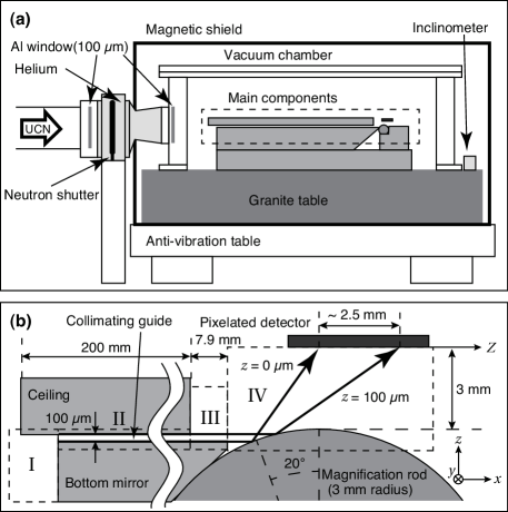
According to Ichikawa2014 , ultracold neutrons, moving in the –direction of the spatial region II with a length between two parallel plane mirrors, separated by a distance , are being prepared in a quantum gravitational state , which is a mixed state of stationary pure quantum gravitational states of ultracold neutrons , where is a principal quantum number and is a moment of time, when ultracold neutrons have been injected into the spatial region II, are random phases. A time–evolution of ultracold neutrons in the spatial region II for should be described by the wave function . Here , where are real functions, and is the binding energy of ultracold neutrons in the –quantum gravitational state between two mirror. A horizontal motion of ultracold neutrons should be, in principle, described by a plane wave , where and are the momentum and energy of a horizontal motion of ultracold neutrons with mass . A horizontal velocity of ultracold neutrons possesses a nearly Gaussian distribution around a mean–value velocity with a variance or a standard deviation Ichikawa2014 . Thus, the wave function of ultracold neutrons in the spatial region II is with .
Passing through the spatial region II between two mirrors ultracold neutrons enter into the spatial region III with a length and restricted by a mirror from below. In the spatial region III the stationary pure quantum gravitational states are described by the wave functions with the binding energies and a principal quantum number . A wave function of the mixed state transforms into the wave function , where are random phases. The coefficients are equal to
| (1) | |||||
where is a moment of time of the crossing of ultracold neutrons boundary between the spatial regions II and III and is a length of the spatial region II (see Fig. 1). We integrate over in the limits , since the wave functions vanish for and . We would like to emphasise that the differences of the binding energies do not vanish, since the binding energies and are always for any principal quantum numbers and . A time evolution of ultracold neutrons in the spatial region III is defined by the wave function . From Eq.(1) one can see that the expansion coefficients depend on random phases only.
Passing through the spatial region III ultracold neutrons arrive at the spatial region IV, where they move above a cylindrical glass rod, which reflects ultracold neutrons as a mirror Ichikawa2014 . A mechanism of our explanation of the experimental data by Ichikawa q et al. Ichikawa2014 is the following. Since ultracold neutrons have a momentum with de Broglie wavelength , they scatter by a cylindrical mirror as classical particles. Due to such a scattering the impact parameters of ultracold neutrons are projected onto a –axis of a horizontal surface of the pixelated detector parallel to the –axis. Since an impact parameter is weighted with the weight , one should observe a specific spatial modulation of a distribution of ultracold neutrons along the –axis, which has been observed by Ichikawa et al. Ichikawa2014 .
III Impact parameter of scattering of ultracold neutrons as classical particles by cylindrical mirror
The ultracold neutrons scatter by a cylindrical mirror with a momentum or with the wavelength . Such a wavelength is much smaller compared with the vertical scale of the region II. Thus, ultracold neutrons scatter by a cylindrical mirror as classical particles. A distribution of ultracold neutrons along the –axis of the pixelated detector is defined by a dependence of the impact parameter on the scattering angle and the parameters of the cylindrical mirror . A dependence of the impact parameter on the scattering angle and the parameters of the cylindrical mirror the radius and the angle Ichikawa2014 is shown in Fig. 2.
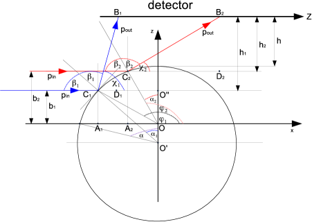
Following the geometry, shown in Fig. 2, one can express the impact parameter as a function of the angle and the azimuthal angle as follows
| (2) |
Since the azimuthal angle and the angle , related to the scattering angle as , are related by
| (3) |
and
| (4) |
in terms of the scattering angle the impact parameter is given by
| (5) |
Since the maximal impact parameter of ultracold neutrons is equal to the height of the region II, i.e. , the minimal scattering angle is (or ). In turn, the maximal scattering angle , defined by the condition , is (or ). Thus, the end–points of the interval are shifted with respect to the points and , defined for the maximal and minimal scattering angle, respectively, as and , where the points and are the projections of the points and , respectively. Thus, a spatial distribution of ultracold neutrons can be observed along the –axis in the interval .
IV Projection of ultracold neutrons with impact parameter onto –axis of pixelated detector
As we have shown in section III ultracold neutrons, moving with an impact parameter with a velocity , are projected by a cylindrical mirror onto the –axis of the pixelated detector. Such a projection we may define as
| (6) |
where for . Using the relations
| (7) |
we obtain as a function of an impact parameter
| (8) |
At we get . Then, taking into account the values of the parameters of the experimental setup of Ichikawa’s experiment Ichikawa2014 we may approximate the impact parameter by the expression
| (9) |
where . At we obtain . Thus, Eq.(9) allows to fit the maximal value of the impact parameter with an accuracy of about . A derivative is
| (10) |
Now we are able to use the impact parameter for the analysis of a spatial distribution of ultracold neutrons by a pixelated detector.
V Spatial distribution of energy levels of quantum gravitational states of ultracold neutrons between two mirrors
For the subsequent analysis of the experimental data by Ichikawa et al. Ichikawa2014 we have to determine a distribution of quantum gravitational states of ultracold neutrons in the spatial region II. The energy levels of the quantum gravitational states of ultracold neutrons are defined by the roots of the equation Ivanov2013
| (11) |
where is the height of the spatial region II, is a quantum scale of quantum gravitational states of ultracold neutrons, where is the gravitational acceleration. The roots of Eq.(11) define the energy levels , where is the principal quantum number and . The maximal number of quantum gravitational states is defined by . Setting , taking into account that we arrive at the equation and and using asymptotic behaviour of the Airy functions for we transcribe Eq.(11) into the form
| (12) |
the root of which
| (13) |
defines the maximal number of quantum gravitational states of ultracold neutrons in the spatial region II.
The same result and the spatial distribution of quantum gravitational levels of ultracold neutrons in the spatial region II we may obtain by following the quasi–classical approximation of quantum mechanics Davydov1965 . In the quasi–classical approximation of quantum mechanics the maximal number of quantum gravitational states of ultracold neutrons in the spatial region is defined by
| (14) |
where is the classical momentum of ultracold neutrons.
Using Eq.(14) we may define the spatial distribution of quantum gravitational levels in the spatial region II. We get
| (15) |
The probability distribution of quantum gravitational states in the spatial region can be given by
| (16) |
where . A probability to find quantum gravitational states in the spatial region is equal to
| (17) |
Below we use this result for the calculation of the expansion coefficients of the wave function of the mixed state of ultracold neutrons in the spatial region II.
Practically our results, obtained above, mean that the spatial distribution of ultracold neutrons between two mirrors is fully defined by the their phase volume. This can be also confirmed by treating ultracold neutrons as an ideal non–relativistic classical gas, confined between two mirrors in the spatial region , with a Maxwell–Boltzmann distribution function in the phase volume at temperature Landau1979 . A Maxwell–Boltzmann distribution function in the phase volume we take in its standard form , where is a total energy of ultracold neutrons. The distribution function is normalised to a total number of ultracold neutrons :
| (18) |
Since for ultracold neutrons , we may replace by unity. This gives
| (19) |
where . Since energy is conserved and at the momentum vanishes, we get and . This results in
| (20) |
that gives a well known result Ruess2000 . For a spatial distribution of ultracold neutrons between two mirrors in the spatial region , normalised to a total number of ultracold neutrons , we obtain following expression
| (21) |
The number of ultracold neutrons in the spatial region is equal to
| (22) |
A spatial distribution of ultracold neutrons Eq.(21) has the same –dependence as the spatial distribution of energy levels of quantum gravitational states of ultracold neutrons.
VI Spatial distribution of probability density of quantum gravitational states of ultracold neutrons
According to Gibbs1975 , ultracold neutrons, moving in the gravitational field of the Earth above a mirror, can be in quantum gravitational states, described by the wave functions equal to Gibbs1975
| (23) |
where , and is a gravitational acceleration. The roots of the Airy function define the energy spectrum of quantum gravitational states in the region III for , where . A spatial distribution of a probability density of ultracold neutrons in a quantum gravitational state with a principal quantum number is equal to or in terms of an impact parameter it is , where is a function of , i.e. (see Eq.(9)). I
As a result, a spatial distribution of a probability density of ultracold neutrons along the –axis in the –excited quantum gravitational state is defined by
| (24) |
The spatial distribution Eq.(24) is defined in the interval . One can show that the probability density Eq.(24) for first twelve quantum gravitational –state, integrated over the region , is equal to unity. For other excited states the probability decreases with increasing.
Now we are able to proceed for a description of the experimental data on a spatial distribution of quantum gravitational states of ultracold neutrons, obtained by Ichikawa et al. Ichikawa2014 . It is obvious that an experimental observation of a spatial distribution of quantum gravitational states of ultracold neutrons in the region III, projected onto the pixelated detector, depends strongly on the wave function of quantum gravitational states of ultracold neutrons in the region II. Below we consider two possibilities for a construction of the wave function of a quantum gravitational state of ultracold neutrons in the region II.
As has been shown in Ivanov2013 , the wave function of the –excited quantum gravitational state of ultracold neutrons, confined in the spatial region between two mirrors, takes the form
| (25) |
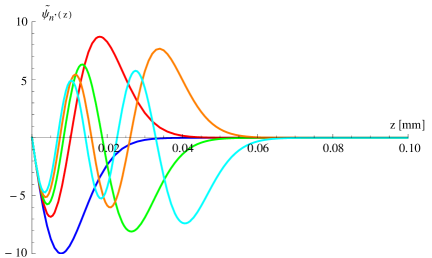
This wave function obeys the constraint caused by the boundary conditions . The roots of Eq.(11) define the energy spectrum for in the region II. One can show that in the region II at height , only first 15 quantum gravitational states are allowed. Ultracold neutrons should be in a mixed state, which is superposition of these 15 allowed quantum gravitational states. As an example,e we plot in Fig. 3 the wave functions of first five quantum gravitational states of ultracold neutrons in the spatial region II. We would like to emphasise that the wave functions of quantum gravitational states of ultracold neutrons in the spatial region II, i.e. for , is very sensitive to the number of digits after comma in the roots of Eq.(11). The calculations of the wave functions of ultracold neutrons in the spatial region II are carried out with the roots of Eq.(11), defined with 200 digits after comma.
For the measurements of the spatial distribution of quantum gravitational states of ultracold neutrons there was used the highest intensity beam line PF2 of ultracold neutrons at ILL UCN1986 . Because ultracold neutrons are distribution in the neutron beam with a probability Eq.(12), the expansion coefficients of 15 quantum gravitational states can be defined by as
| (26) |
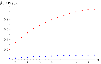
and normalised to unity , where and are random phases. In the right plot of Fig. 3 we show the probabilities and to find the –quantum gravitational state of ultracold neutrons in the spatial region II, which we name quantum and classical probabilities, respectively.
For the analysis of a spatial distribution of the quantum gravitational states of ultracold neutrons in the region III we have to expand the wave function in the region II in terms of the wave functions . The expansion coefficients (see section I) are equal to
| (27) |
where is a moment of time of the crossing of ultracold neutrons boundary between the spatial regions II and III, is a length of the spatial region II (see Fig. 1) and . As has been pointed out above the expansion coefficients of the wave function do not depend on the random phase . Averaging over the random phases we obtain the spatial distribution of probability density of the quantum gravitational states of ultracold neutrons
| (28) |
where , the probability to find a quantum gravitational state of ultracold neutrons in the mixed state with the wave function in the spatial region III. is given by
| (29) |
The probabilities are normalised by
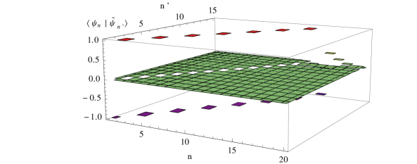
| (30) |
where we have used the completeness condition
| (31) |
For a numerical analysis we use first 100 quantum gravitational states in the region III. This allows to obtain the right hand side (r.h.s.) of Eq.(35) equal to .
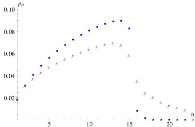
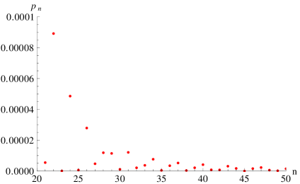
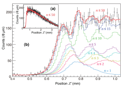
The probabilities to find ultracold neutrons in the –quantum gravitational state in the spatial region III are plotted in Fig. 4. In the left figure we give the probabilities for . In the figure we specify a behaviour of the probabilities for . We show that they are small and random oscillate. In the figure down we compare the probabilities , calculated in our paper (blue dots) and obtained by Ichikawa et al. (red crosses). One may see that there is an agreement only for first two gravitational states. On the whole our probabilities disagree with those by Ichikawa et al..
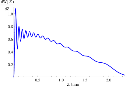
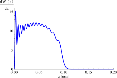
Substituting Eq.(VII) into Eq.(28) we obtain a spatial distribution of quantum gravitational states of ultracold neutrons in the spatial region III. In Fig. 5 we plot a spatial distribution of quantum probabilities of ultracold neutrons, projected onto the pixelated detector (left) and in the spatial region III (right). The shapes of these theoretical distributions disagree with the shape of the experimental one, shown in Fig. 5 (down).
As a result one may conclude that the experimental data by Ichikawa et al. Ichikawa2014 have no relation to a spatial distribution of quantum gravitational states of ultracold neutrons. In the section VII we confirm our assertion by analysing a behaviour of the Wigner function.
VII Wigner function for quantum gravitational states of ultracold neutrons
In this section we analyse a spatial distribution of quantum gravitational states of ultracold neutrons in terms of the Wigner function Wigner1932 as it has been performed by Ichikawa et al. Ichikawa2014 . The Wigner function for quantum gravitational states of ultracold neutrons in the region III is defined by Ichikawa2014
| (32) |
where . Replacing (see Eq.(11)) and , where is
| (33) |
and in terms of the expansion coefficients and the wave functions we transcribe the Wigner function into the form
| (34) |
where is defined by Eq.(11), the coefficients and are given by Eq.(24)). The coefficients , averaged over random phases , are
| (35) |
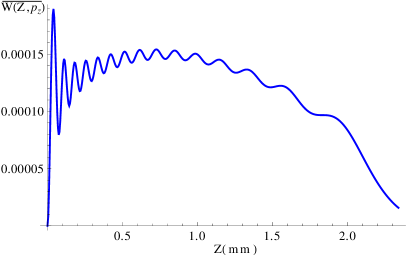
where , , and . The Wigner function Eq.(VII) is plotted in Fig 6.
Having integrated the Wigner function Eq.(VII) over the velocities with a Gaussian distribution, w arrive at the expression
| (36) |
where is a variance horizontal velocities of ultracold neutrons. The contributions of the crossing terms and can be neglected because of strong oscillations and smallness of the amplitudes of oscillations. Replacing and using Eq.(11) we obtain in terms of the Wigner function a spatial distribution of quantum gravitational states of ultracold neutrons in a pixelated detector
| (37) | |||||
In Fig. 7 we plot the Wigner function in the interval .
VIII Conclusion
We have analysed the experimental data on a spatial distribution of quantum gravitational states of ultracold neutrons, obtained by Ichikawa et al. Ichikawa2014 . According to the experimental setup of Ichikawa et al. Ichikawa2014 , ultracold neutrons with a horizontal velocity , having a Gaussian distribution with a mean velocity and a variance , pass through i) first a spatial region between two parallel mirrors, ii) second a spatial region above a mirror and then iii) are detected by the detector. The projection of ultracold neutrons from the spatial region above the mirror onto the detector is carried out by the cylindrical mirror.
Because of a smallness of the de Broglie wavelength in comparison with the distance between two mirror and the size of the cylindrical mirror with radius ultracold neutrons scatter by the cylindrical mirror as classical particles. An impact parameter of ultracold neutrons is equal to the vertical –variable. For the analysis of the spatial distribution of ultracold neutrons by the detector we have projected ultracold neutrons with an impact parameter onto the detector, characterised by the variable . We have found that for the experimental setup Ichikawa2014 ultracold neutrons, scattered by the cylindrical mirror, can be detected only at the interval . We have carried out a projection in such a way that ultracold neutrons with the impact parameter are projected onto .
For the calculation of the probability distribution densities of quantum gravitational states of ultracold neutrons and the Wigner functions we have defined the wave function of the mixed state in the spatial region II between two mirrors as a superposition of 15 quantum gravitational states with the expansion coefficients (), defined by the –distribution of ultracold neutrons. The wave functions of quantum gravitational states of ultracold neutrons between two mirrors have been calculated in Ivanov2013 . In the subsequent expansion of the wave function of ultracold neutrons in the mixed state into the set of quantum gravitational states of ultracold neutrons in the spatial region III above the mirror we have restricted such an expansion by one hundred states with the expansion coefficients (), which fit well the unitarity condition , where we have averaged over the random phases of the expansion coefficients of the mixed quantum gravitational state of ultracold neutrons between two mirrors in the spatial region II.
In Fig. 5 we show that the probabilities to find ultracold neutrons in the –excited quantum gravitational state, calculated in our paper, differ from the probabilities, calculated by Ichikawa et al. Ichikawa2014 . The smooth dpendence on the principal quantum number of the probabilities for , obtained by Ichikawa et al. Ichikawa2014 , is incorrect, since the wave function of the mixed state is localised in the region and the probabilities for show irregular and oscillating character of the dependence on the principal quantum number .
We have shown that the probability distribution densities of quantum gravitational states Fig. 6 and the Wigner function Fig. 7 do not fit the experimental data by Ichikawa et al. Ichikawa2014 . This may imply that the experimental data by Ichikawa et al. Ichikawa2014 cannot be explained as the spatial distribution of quantum gravitational states of ultracold neutrons in the sense of our description.
IX Acknowledgement
We want to thank our dear colleague Andrey Nikolaevich Ivanov, who was the main investigator of this work until he sadly passed away on December 18, 2021. We see it as our professional and personal duty to honor his legacy by continuing to publish our collaborative work. Andrey was born on June 3, 1945 in what was then Leningrad. Since 1993 he was a university professor at the Faculty of Physics, named ”Peter The Great St. Petersburg Polytechnic University” after Peter the Great. Since 1995 he has been a guest professor at the Institute for Nuclear Physics at the Vienna University of Technology for several years and has been closely associated with the institute ever since. This is also were we met Andrey and have been collaborating with him closely over more than 20 years resulting in 40 scientific publications, see also Ivanov:2013fca ; Ivanov2013a ; Ivanov2014 ; Ivanov2014a ; Ivanov:2017mnz ; Ivanov:2017wxl ; Ivanov2017b ; Ivanov:2018uuk ; Ivanov:2018vit ; Ivanov:2018vmz ; Ivanov:2018qen ; Ivanov:2018ngi ; Ivanov:2018olo ; Ivanov:2018yir ; Ivanov:2019rkp ; Ivanov:2019bqr ; Ivanov:2020ybx ; Ivanov:2021bae ; Ivanov:2021lji ; Ivanov:2021yhl ; Ivanov:2021xkm . We will miss Andrey as a personal friend and his immense wealth of ideas, scientific skills and his creativity. See also the official obituary for Andrey Nikolaevich Ivanov.
R.Höllwieser is receiving funding from the program ” Netzwerke 2021”, an initiative of the Ministry of Culture and Science of the State of Northrhine Westphalia, in the NRW-FAIR network, funding code NW21-024-A. B 128/5-2. The work of M. Wellenzohn was supported by MA 23 (p.n. 27-07 and p.n. 30-22). The sole responsibility for the content of this publication lies with the authors.
References
- (1) R. L. Gibbs, Am. J. Phys. 43, 25 (1975); J. Gea–Banacloche, Am. J. Phys. 67, 776 (1999); H. Wallis et al., Appl. Phys. B 54, 407 (1992).
- (2) V. V. Nesvizhevsky, H. G. Börner, A. K. Petukhov, H. Abele, S. Baeßler, F. J. Rueß, Th. Stöferle, A. Westphal, A. M. Gagarski, G. A. Petrov, and A. V. Strelkov, Nature 415, 297 (2002).
- (3) V. V. Nesvizhevsky, H. G. Börner, A. M. Gagarski, A. K. Petukhov, G. A. Petrov, H. Abele, S. Baeßler, G. Divkovic, F. J. Rueß, Th. Stöferle, A. Westphal, A. V. Strelkov, K. V. Protasov, and A. Yu. Voronin, Phys. Rev. D 67, 102002 (2003).
- (4) V. V. Nesvizhevsky, A. K. Petukhov, H. G. Börner, T. A. Baranova, A. M. Gagarski, G. A. Petrov, K. V. Protasov, A. Yu. Voronin, S. Baeßler, H. Abele, A. Westphal, and L. Lucovac, Eur. Phys. J. C 40, 479 (2005).
- (5) A. Westphal, H. Abele, S. Baeßler, V. V. Nesvizhevsky, A. K. Petukhov, K. V. Protasov, and A. Yu. Voronin, Eur. Phys. J. C 51, 367 (2007).
- (6) H. Abele, T. Jenke, H. Leeb, J. Schmiedmayer, Phys. Rev. D 81, 065019 (2010).
- (7) T. Jenke, P. Geltenbort, H. Lemmel, and H. Abele, Nature Phys. 7, 468 (2011).
- (8) H. Abele, T. Jenke, D. Stadler, and P. Geltenbort, Nucl. Phys. A 827, 593c (2009).
- (9) T. Jenke, D. Stadler, H. Abele, and P. Geltenbort, Nucl. Instr. and Meth. in Physics Res. A 611, 318 (2009).
- (10) H. Abele and H. Leeb, New J. Phys. 14, 055010 (2012).
- (11) T. Jenke, G. Cronenberg, J. Burgdörfer, L. A. Chizhova, P. Geltenbort, A. N. Ivanov, T. Lauer, T. Lins, S. Rotter, H. Saul, U. Schmidt, and H. Abele, Phys. Rev. Lett. 112, 151105 (2014).
- (12) A. N. Ivanov, R. Höllwieser, T. Jenke, M. Wellenzohn, and H. Abele, Phys. Rev. D 87, 105013 (2013).
- (13) G. Ichikawa, S. Komamiya, Y. Kamiya, Y. Minami, M. Tani, P. Geltenbort, K. Yamamura, M. Nagano, T. Sanuki, S. Kawasaki, M. Hino, and M. Kitaguchi, Phys. Rev. Lett. 112, 071101 (2014), arXiv: 1304.1660v4 [hep-ex].
- (14) E. P. Wigner, Phys. Rev. 40, 749 (1932); M. Hillery, R. F. O’Connel, M. O. Scully, and E. P. Wigner, Phys. Rev. 106, 121 (1984).
- (15) A. S. Davydov, in Quantum mechanics, Pergamon Press, Oxford, 1965.
- (16) L. D. Landau und E. M. Lifschitz, in Lehrbuch der theoretischen Physik, Band I, Mechanik, Verlag Harri Deutsch, Frankfurt am Main, 2007.
- (17) A. Steyerl et al., Phys. Lett. A 116, 347 (1986).
- (18) L. D. Landau und E. M. Lifschitz, in Lehrbuch der theoretischen Physik, Band V, Statistische Physik, Teil 1 von E. M. Lifschitz und L. P. Pitajewski, Akademie Verlag Berlin, s. 107, 1979.
- (19) F. Ruess, Diploma thesis, Faculty of Physics and Astronomy, University of Heidelberg, August 2000.
- (20) A. N. Ivanov, R. Höllwieser, N. I. Troitskaya, and M. Wellenzohn. Proton recoil energy and angular distribution of neutron radiative -decay. Phys. Rev., D88(6):065026, 2013.
- (21) A. N. Ivanov, R. Höllwieser, N. I. Troitskaya, M. Wellenzohn, O.M. Zherebtsov, and A. P. Serebrov, Deficit of reactor antineutrinos at distances smaller than 100 m and inverse beta decay, Phys. Rev. C 88, 055501 (2013).
- (22) A. N. Ivanov, M. Pitschmann, N. I. Troitskaya, and Ya. A. Berdnikov, Bound-state beta decay of the neutron re-examined, Phys. Rev. C 89, 055502 (2014).
- (23) A. N. Ivanov, R. Höllwieser, M. Wellenzohn, N. I. Troitskaya, and Ya. A. Berdnikov, Internal bremsstrahlung of beta decay of atomic , Phys. Rev. C 90, 064608 (2014).
- (24) A. N. Ivanov, R. Höllwieser, N. I. Troitskaya, M. Wellenzohn and Y. A. Berdnikov, Precision analysis of electron energy spectrum and angular distribution of neutron decay with polarized neutron and electron, Phys. Rev. C 95, no.5, 055502 (2017), [erratum: Phys. Rev. C 104, no.6, 069901 (2021)] doi:10.1103/PhysRevC.104.069901, [arXiv:1705.07330 [hep-ph]].
- (25) A. N. Ivanov, R. Höllwieser, N. I. Troitskaya, M. Wellenzohn and Y. A. Berdnikov, Precision theoretical analysis of neutron radiative beta decay to order ,’ Phys. Rev. D 95, no.11, 113006 (2017) doi:10.1103/PhysRevD.95.113006 [arXiv:1706.08687 [hep-ph]].
- (26) A. N. Ivanov, R. Höllwieser, N. I. Troitskaya, M. Wellenzohn, and Ya. A. Berdnikov, Precision analysis of electron energy spectrum and angular distribution of neutron beta decay with polarized neutron and electron, Phys. Rev. C 95, 055502 (2017).
- (27) A. N. Ivanov, R. Höllwieser, N. I. Troitskaya, M. Wellenzohn and Y. A. Berdnikov, Neutron dark matter decays and correlation coefficients of neutron -decays, Nucl. Phys. B 938, 114-130 (2019), doi:10.1016/j.nuclphysb.2018.11.005, [arXiv:1808.09805 [hep-ph]].
- (28) A. N. Ivanov, R. Höllwieser, N. I. Troitskaya, M. Wellenzohn and Y. A. Berdnikov, Neutron Dark Matter Decays, [arXiv:1806.10107 [hep-ph]].
- (29) A. N. Ivanov, R. Höllwieser, N. I. Troitskaya, M. Wellenzohn and Y. A. Berdnikov, Tests of the standard model in neutron decay with a polarized neutron and electron and an unpolarized proton, Phys. Rev. C 98, no.3, 035503 (2018) doi:10.1103/PhysRevC.98.035503 [arXiv:1805.03880 [hep-ph]].
- (30) A. N. Ivanov, R. Höllwieser, N. I. Troitskaya, M. Wellenzohn, and Ya A. Berdnikov. Gauge Properties of Hadronic Structure of Nucleon in Neutron Radiative Beta Decay to Order O() in Standard V - A Effective Theory with QED and Linear Sigma Model of Strong Low–Energy Interactions. Int. J. Mod. Phys. A, 33(33):1850199, 2018.
- (31) A. N. Ivanov, R. Höllwieser, N. I. Troitskaya, M. Wellenzohn, and Ya A. Berdnikov. Gauge and infrared properties of hadronic structure of nucleon in neutron beta decay to order in standard effective theory with QED and linear sigma model of strong low-energy interactions. Int. J. Mod. Phys. A, 34(02):1950010, 2019.
- (32) Andrey N. Ivanov, Roman Höllwieser, Nataliya I. Troitskaya, Markus Wellenzohn, and Ya A. Berdnikov. Electrodisintegration of Deuteron into Dark Matter and Proton Close to Threshold. Symmetry, 13(11):2169, 2021.
- (33) A. N. Ivanov, R. Höllwieser, N. I. Troitskaya, M. Wellenzohn, and Ya A. Berdnikov. Tests of the standard model in neutron beta decay with polarized electrons and unpolarized neutrons and protons. Phys. Rev. D, 99(5):053004, 2019. [Erratum: Phys.Rev.D 104, 059902 (2021)].
- (34) A. N. Ivanov, R. Höllwieser, N. I. Troitskaya, M. Wellenzohn, and Ya. A. Berdnikov. Radiative corrections of order to Sirlin’s radiative corrections of order to the neutron lifetime. Phys. Rev. D, 99(9):093006, 2019.
- (35) A. N. Ivanov, R. Höllwieser, N. I. Troitskaya, M. Wellenzohn, and Ya. A. Berdnikov. Precision analysis of pseudoscalar interactions in neutron beta decays. Nucl. Phys. B, 951:114891, 2020.
- (36) A. N. Ivanov, R. Höllwieser, N. I. Troitskaya, M. Wellenzohn, and Ya. A. Berdnikov. Corrections of order , caused by weak magnetism and proton recoil, to the neutron lifetime and correlation coefficients of the neutron beta decay. Results Phys., 21:103806, 2021.
- (37) A. N. Ivanov, R. Höllwieser, N. I. Troitskaya, M. Wellenzohn, and Ya. A. Berdnikov. Radiative corrections of order to Sirlin’s radiative corrections of order , induced by the hadronic structure of the neutron. Phys. Rev. D, 103(11):113007, 2021.
- (38) A. N. Ivanov, R. Höllwieser, N. I. Troitskaya, M. Wellenzohn, and Ya. A. Berdnikov. Theoretical description of the neutron beta decay in the standard model at the level of 10-5. Phys. Rev. D, 104(3):033006, 2021.
- (39) A. N. Ivanov, R. Höllwieser, N. I. Troitskaya, M. Wellenzohn, and Ya. A. Berdnikov. Structure of the correlation coefficients and of the neutron decay. Phys. Rev. C, 104(2):025503, 2021.
- (40) A. N. Ivanov, R. Höllwieser, N. I. Troitskaya, M. Wellenzohn, and Ya. A. Berdnikov. On the correlation coefficient of the neutron beta decay, caused by the correlation structure invariant under discrete P, C and T symmetries. Phys. Lett. B, 816:136263, 2021.