Deep Blind Super-Resolution for Satellite Video

Abstract

Recent efforts have witnessed remarkable progress in Satellite Video Super-Resolution (SVSR). However, most SVSR methods usually assume the degradation is fixed and known, e.g., bicubic downsampling, which makes them vulnerable in real-world scenes with multiple and unknown degradations. To alleviate this issue, blind SR has thus become a research hotspot. Nevertheless, existing approaches are mainly engaged in blur kernel estimation while losing sight of another critical aspect for VSR tasks: temporal compensation, especially compensating for blurry and smooth pixels with vital sharpness from severely degraded satellite videos. Therefore, this paper proposes a practical Blind SVSR algorithm (BSVSR) to explore more sharp cues by considering the pixel-wise blur levels in a coarse-to-fine manner. Specifically, we employed multi-scale deformable convolution to coarsely aggregate the temporal redundancy into adjacent frames by window-slid progressive fusion. Then the adjacent features are finely merged into mid-feature using deformable attention, which measures the blur levels of pixels and assigns more weights to the informative pixels, thus inspiring the representation of sharpness. Moreover, we devise a pyramid spatial transformation module to adjust the solution space of sharp mid-feature, resulting in flexible feature adaptation in multi-level domains. Quantitative and qualitative evaluations on both simulated and real-world satellite videos demonstrate that our BSVSR performs favorably against state-of-the-art non-blind and blind SR models. Code will be available at https://github.com/XY-boy/Blind-Satellite-VSR

I Introduction

Video satellite has recently received increasing attention due to its strength in dynamic observations. Nowadays, satellite video imagery is widely used in remote sensing tasks with high temporal variations [1], such as object tracking [2], anomaly detection [3, 4], classification [5, 6, 7, 8, 9, 10], change detection [11], etc. However, the satellite platform tremors and atmosphere scatters in the remote imaging process often generate undesirable blurs in satellite videos. Additionally, the spatial resolution of satellite video is usually degraded to stabilize the remote transmission. As a result, the visual quality of satellite video is inevitably contaminated, which results in performance drops in subsequent applications. Therefore, it is of practical significance to improve the spatial resolution of satellite video for both human perception and downstream tasks.

Compared to hardware upgrades, Super-Resolution (SR) technology provides an optimal solution for this highly ill-posed problem [12, 13, 14, 15, 16]. Traditional SR methods [17] often employ hand-crafted priors to make this problem well-posed. However, these methods are fragile to the laborious priors and may restore unsatisfactory results because the real constraint often deviates from the predefined priors. Besides, they also suffer from high computational complexity and can lead to sub-optimal performance.

Benefit from the development of deep neural networks (DNNs) [18, 19, 20], especially the huge success in low-level vision tasks [21, 22, 23, 24, 25], the deep-learning-based SR approaches are booming. In spite of achieving decent results, most of them are specialized for single and known degradation, e.g., bicubic downsampling, and tend to collapse in real-scene. Therefore, more efforts have been paid to blind SR approaches, which address the SR problem under multiple and unknown degradations, e.g., unknown blur kernels, and downsamplings. Recently, numerous works have made promising progress on blind Single Image Super-Resolution (SISR). However, they are less applicable in satellite videos as the additional information in the temporal domain is not fully explored. More recently, some scholars have investigated blind Video Super-Resolution (VSR). Nevertheless, these methods focus solely on accurate blur kernel estimation while overlooking the significance of temporal compensation in VSR, especially precise compensation for blurry and smooth pixels in severely degraded frames.

Generally, existing blind VSR approaches typically utilize optical flow warping for temporal compensation. However, they are laborious in large-scale satellite imagery and not robust in complex imaging scenarios with scale variations and sparse motions. What’s worse, in blind SR settings, the appearance of satellite video frames is severely blurred and downsampled, which poses more challenges for accurate flow estimation. Liu et al. [26] proposed a joint estimation network, which adopts patch matching to realize patch-by-patch alignment. However, the patch-wise alignment does not fully exploit the sub-pixel redundancy. Moreover, the high-similarity patch may also contain blurry pixels. Simply aggregating them to mid-feature is not sophisticated to consider the blur level of pixels, which may introduce and amplify the blurry information and restore unsatisfactory results. Overall, two issues hinder us from moving forward:

1. Existing temporal compensation strategies are time-consuming and not robust in severely degraded satellite videos.

2. Lacking elaborate pixel-wise temporal modeling to grasp vital sharpness and eliminate unfavorable blurs.

Although the pixels may be degraded by the same degree of blurring, they are still not equally informative to the recovery of the clean and HR. Therefore, we define sharp pixels as those that can provide more clean and sharp cues (e.g., high-frequency texture), which are beneficial for reconstruction. To address the issues mentioned above, a more practical manner is urgently needed to consider the blur level of pixels and explore more sharp and clean clues for temporal compensation. Inspired by previous research, Deformable Convolution (DConv) is a preferable choice in satellite videos as it benefits from adaptive pixel-wise sampling to mitigate the misalignment caused by inaccuracy optical flow estimation. However, the learned pixels in deformable sampling points are also blurry and not equally informative for restoring sharp details. Very recently, [27] has investigated the contribution of different sampling positions for efficient spatial element relationship modeling. This motivates us to model the different blurry levels of pixels with the equipment of deformable attention. Hence, we could effectively aggregate the deformable sampling points by encouraging the representation of sharp pixels and eliminating the effects of blurry pixels.

In particular, this paper proposes a novel approach (BSVSR) to progressively aggregate sharp information while considering the pixel-wise blur level. We adopt the efficient Multi-Scale Deformable convolution (MSD) alignment [28] to explore multi-scale temporal redundancy from the entire frame sequence with window-slid progressive fusion. This helps to alleviate the alignment pressure brought by large displacements. To finely aggregate the sharp mid-feature, a multi-scale Deformable Attention (DA) module was proposed to measure the pixel-wise blur level, which is practical to assign more attention to clean and sharp pixels for better sharpness representation. Benefiting from the coarse-to-fine manner, we can favorably identify the critical sharpness from severely blurred and downsampled satellite videos. To flexibly adjust the solution space and make the sharp mid-feature adaptive to various degradation, a Pyramid Spatial Transform (PST) strategy is established. With pyramid design, we could improve the diversity of mid-feature with multi-level spatial activation, making the transformation aware of multi-scale spatial distribution in satellite videos.

To sum up, our contributions are listed as follows:

1) Different from previous optical-flow-based and patch-wise compensation methods, we propose to aggregate sharp information in severely degraded satellite videos with progressive temporal compensation, which exploits Multi-Scale Deformable (MSD) convolution and Deformable Attention (DA) to explore more sharp and clean clues by considering the blur level of pixels.

2) To achieve flexible feature adaptation, we develop a robust Pyramid Spatial Transform (PST) module, where blur information could be transformed into mid-feature in multi-level feature domains.

3) Extensive experiments are conducted on Jilin-1, Carbonite-2, UrtheCast, Skysat-1, and Zhuhai-1 video satellites. And the results demonstrate our BSVSR performs favorably against state-of-the-art blind and non-blind SR approaches.

The remainder of this paper is organized as follows: Section II reviews the progress of video super-resolution, Section III involves details of our approach, Section IV includes extensive experiments and analysis, and Section V is the conclusion.

II Related Work

II-A Deep-Learning-based Classical Super-Resolution

We first review the classical SR as it lays the foundation of blind SR. Classical SR methods often assume that the degradation process is single and known, such as bicubic downsampling.

II-A1 Classical SISR methods

With the success of SRCNN [29], CNN-based SISR methods have been blooming, with remarkable progress in deeper networks [30], attention-based networks [31], recurrent networks [32] and recent popular transformer-based models [33, 34]. Although they achieved decent results in bicubic-downsampled images, they are not capable of handling multiple degradations. Also, lacking consideration of temporal redundancy makes SISR less generalized in VSR tasks.

II-A2 Classical VSR methods

The key success of VSR tasks is to compensate the pixels of the mid-frame with the temporal redundancy along frames. According to the type of temporal compensation, classical VSR can be broadly divided into flow-based and kernel-based compensation.

Flow-based Compensation. This approaches [35, 36, 37] employs explicit optical flow to describe the motion relationships between frames and perform frame/feature-wise warping to align the adjacent frame to mid-frame. As mentioned in [26], optical flow estimation is time-consuming and not robust in blurry and low-resolution videos. Thus, the kernel-based method may provide a more efficient optimal for VSR task, benefiting from its adaptive learning capability.

Kernel-based Compensation. Such methods often implicitly involve the compensation into learnable parameters. Jo et al. [38] proposed to directly learn a 3D upsampling filter (DUF) to super-resolve each LR pixel. To reduce the high computational consumption of 3D CNN, Tian et al. [39] introduce an efficient deformable network to explore more temporal priors with deformable sampling points. Later, more efforts have been paid to generating precise offset parameters for deformable sampling, such as pyramid [40] and multi-scale [41] architectures. Some works employ the attention mechanism to find out valuable complementary. Yu et al. [42] established a novel cross-frame non-local attention and memory-augment attention (MANA) to memorize more details in mid-feature. Recently, some recurrent networks [43, 44] proposed to recurrently propagate temporal information for better compensation.

Although kernel-based approaches could realize adaptive compensation at the pixel level, they rarely consider the blur level of pixels and treat them equally, thus failing to find the most useful sharp cues which are beneficial for restoration.

II-B Deep-Learning-based Blind Super-Resolution

Depending on whether apparent blur information is transformed, these kinds of methods can be subdivided into explicit and implicit blur transformation.

Explicit Blur Transformation. Early work [45] encoded the explicit blur kernels into feature maps and simply concatenated them with LR features. However, they only allow partial transformation. Later, [46] proposed a deep Unfolding Super-resolution Network (USRNet), which transforms the blur kernel by unfolding the optimization problem. To mitigate the performance drop caused by the mismatch between the estimated blur kernel and the realistic one, [47] established an iterative kernel correct network (IKC) to adaptively refine the predicted blur kernel. In addition, they further proposed a Spatial Feature Transformation (SFT) layer to profoundly transform the blur information into features for the adaptive SR process. Particularly, the blur kernel is exploited to guide the shift and scaling of LR features, which helps the LR features to adapt to a suitable domain for reconstruction. Currently, the SFT layer has been commonly used for blur transformation. However, it still lacks flexibility in modulating the spatial and channel of deep features. Recently, Wang et al. [48] presented a Degradation-Aware Convolution (DAConv) to achieve deep blur transformation in two branches. In spatial branches, they use depth-wise convolution to integrate the blur representations into the LR feature. In the channel branch, channel attention was introduced for channel-wise modulation.

Implicit Blur Transformation. Such methods mainly grasp implicitly learning the domain distribution from external datasets. Jo et al. [49] implicitly learned an adaptive generator (AdaTarget) to upsample LR images with diverse unknown blur kernels. Similarly, some efforts [50, 51, 52] have been made to achieve cross-domain learning with Generative Adversarial Networks (GAN). However, the implicit transformation faces harsh convergence conditions as GAN-based models are easy to collapse and produce undesirable artifacts [53].

In summary, the explicit blur transformation is mainstream because they are straightforward and easy to train. Nevertheless, adapting the feature to a desired domain still remains a challenging problem.

II-C Blind Super-Resolution for Satellite Video

Most early works are SISR approaches [54, 55, 56, 57, 58]. However, their performance has reached a plateau without exploring the temporal information. To grasp the temporal redundancy in satellite videos [59], Liu et al. [60] proposed a traditional VSR framework, which uses the non-local temporal similarity as priors to constrain the solution space. He et al. [61] employ 3D convolution to achieve temporal compensation, which is not elaborate in exploring the temporal priors. Xiao et al. [28] developed a multi-scale DConv for precise alignment and proposed a temporal grouping projection to fuse the aligned features. To explore the spatial-temporal collaborative redundancy, they put forward a flow-DConv deeply coupled strategy [62] and enhance the temporal information by a spatial-temporal transformer. Recently, Jin et al. [63] introduced both transformer and CNN to fully excavate the local and global redundancy. Xiao et al. [64] developed a novel framework that exploits temporal difference to realize temporal compensation. Although these methods perform favorably on bicubic-downsampled satellite videos, it is less generalized in blind degradation settings, e.g., unknown blurs and downsampling.

Towards this end, some blind super-resolution approaches [65, 66] have thus become a hot spot. Liu et al. [26] further proposed a joint estimation network for collaborative optimization of blur kernel estimation and SR process. He et al. [67] develop a ghost-module network for blind satellite VSR. However, they both lose sight of precise temporal compensation in severely blurry and low-resolution satellite videos. In fact, not all pixels are clean and sharp and beneficial for blind VSR. Therefore, we still need to move forward by compensating more clean and sharp cues for blurry and smooth pixels.

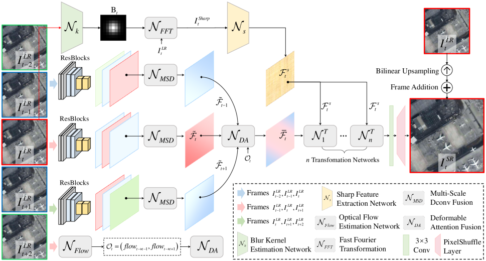
Figure 1: The overview of our BSVSR, which takes $2N+1=5$ consecutive blurry low-resolution frames as input and predicts the sharp high-resolution mid-frame $I^{SR}_{t}$.

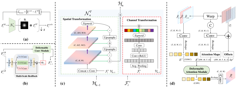
Figure 2: The flowchart of (a) the optimization of blur kernel estimation network; (b) Multi-Scale Deformable (MSD) convolution alignment [28] used for coarse compensation; (c) n-th blur-aware transformation network, which receives blur-aware feature ${\rm{{\cal F}}}_{t}^{s}$ and the result of previous transformation ${{\rm{{\cal H}}}_{n-1}}$ and outputs ${{\rm{{\cal H}}}_{n}}$; (d) Deformable Attention (DA) used for fine compensation.

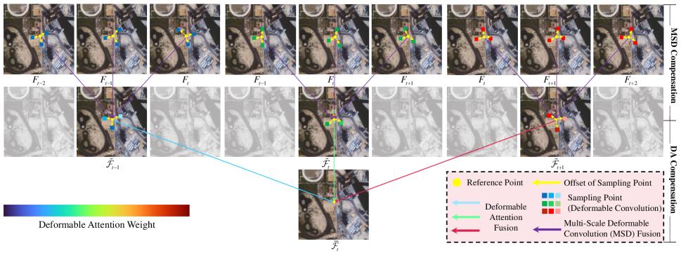
Figure 3: The illustration of the proposed progressive temporal compensation strategy, which used Multi-Scale Deformable convolution (MSD) compensation and Deformable Attention (DA) fusion to explore more clean and sharp cues in a coarse-to-fine manner. The color of the sampling points represents the attention weights used for aggregation. By assigning higher attention weights to clean and sharp points, we can encourage the representation of vital sharpness and eliminate blurry pixels.

III Methodology

III-A Degradation Formulation

Let $I^{LR}_{t}$ be the degraded mid-frame. The degradation process of $I^{LR}_{t}$ can be formulated by the following:

$$I_{t}^{LR}={\left({I_{t}^{GT}\otimes B}\right)_{\downarrow s}}+N,$$ (1)

where $I_{t}^{GT}$ represents the HR ground-truth mid-frame, $B$ is a 2D blur kernel filter, $\otimes$ means convolution, $\downarrow s$ denotes spatial downsampling operation with a scale factor of $s$ and $N$ is the noise term. Following previous works [26], this paper only focuses on blur and downsampling degradations, which means $N=0$. And we set $B$ to isotropic Gaussian blur kernel and $\downarrow s$ to $\times s$ bicubic downsampling.

III-B Overview

The proposed network ${f_{{\mathop{\rm BSVSR}\nolimits}}}\left(\cdot\right)$ aims to recover a clean and sharp high-resolution (HR) mid-frame $I^{SR}_{t}$ given $2N+1$ consecutive blurry LR frames ${\rm I}=\left\{{I_{t+n}^{LR}}\right\}_{n=-N}^{N}$. That is:

$$I_{t}^{SR}={f_{{\mathop{\rm BSVSR}\nolimits}}}\left({\rm I}\right).$$ (2)

As shown in Fig. 1, we set $N=2$ for a brief illustration. Firstly, we perform blur estimation to generate blur-aware feature ${\rm{{\cal F}}}_{t}^{s}$ through ${{\rm{{\cal N}}}_{k}}$, ${{\rm{{\cal N}}}_{FFT}}$ and ${{\rm{{\cal N}}}_{s}}$. Secondly, the blurry LR frames will be progressively compensated to sharp mid-feature ${\rm{{\cal F}}}_{t}^{s}$ by multi-scale deformable convolution ${{\rm{{\cal N}}}_{MSD}}$ and multi-scale deformable attention ${{\rm{{\cal N}}}_{DA}}$ in a coarse-to-fine manner. Thirdly, ${\rm{{\cal F}}}_{t}^{s}$ is transformed into ${{\rm{\bar{\cal F}}}_{t}}$ to guide the sharp mid-feature adaptive to a desired domain for reconstruction. Denote the output of $n$-th transformation ${\rm{{\cal N}}}_{n}^{T}$ as ${{\rm{{\cal H}}}_{n}}$.

Finally, we set a $3\times 3$ convolution and a pixel-shuffle layer to restore the super-resolved mid-frame from ${{\rm{{\cal H}}}_{n}}$.

In the following subsections, we will introduce the implementation details of our BSVSR.

III-C Blur Estimation

We follow the blur estimation process in [68] as it offers decent performance with a lightweight design. Firstly, we employ kernel estimation network ${{\rm{{\cal N}}}_{k}}$ to predict the explict blur kernel ${{\mathop{\rm B}\nolimits}_{t}}$ from $I_{t}^{LR}$.

$${{\mathop{\rm B}\nolimits}_{t}}={{\rm{{\cal N}}}_{k}}\left({I_{t}^{LR}}\right).$$ (3)

As shown in Fig. 2 (a), the estimated blur kernel is used to generate $I^{cycle}_{t}$. ${{\rm{{\cal N}}}_{k}}$ is trained by optimalize the $L_{1}$ difference between $I^{cycle}_{t}$ and $I^{LR}_{t}$. After training of ${{\rm{{\cal N}}}_{k}}$, a Fast Fourier Transformation strategy ${{\rm{{\cal N}}}_{FFT}}$ is adopted to explore the latent sharp mid-frame $I_{t}^{sharp}$.

$$I_{t}^{sharp}={{\rm{{\cal N}}}_{FFT}}\left({I_{t}^{LR},{{\mathop{\rm B}\nolimits}_{t}}}\right)$$ (4)

Through a sharp feature extraction network ${{\rm{{\cal N}}}_{s}}$, we obtain a blur-aware mid-feature ${\rm{{\cal F}}}_{t}^{s}$ that contains blur information.

$${\rm{{\cal F}}}_{t}^{s}={{\rm{{\cal N}}}_{s}}\left({I_{t}^{sharp}}\right)$$ (5)

Note that blur estimation is not the major focus of our paper and we pay more attention on accurate compensation for blurry LR frames. More details about ${{\rm{{\cal N}}}_{k}}$, ${{\rm{{\cal N}}}_{FFT}}$ and ${{\rm{{\cal N}}}_{s}}$ can be found at [68].

III-D Coarse-to-fine Progressive Compensation

Previous blind VSR methods use optical flow warping to align adjacent frames to mid-frame for compensation, which tends to introduce inaccurate motions in severely blurred LR satellite frames. To mitigate the misalignment and extract sharp information, we proposed a progressive compensation strategy that aggregates LR features in a coarse-to-fine manner. As shown in Fig. 3, it consists of two stages, termed Multi-Scale Deformable convolution (MSD) compensation and Deformable Attention (DA) compensation. Before performing compensation, $2N+1$ consecutive frames ${\rm I}$ will be extracted to LR features $\left\{{F_{t+n}^{LR}}\right\}_{n=-N}^{N}$.

Multi-Scale Deformable convolution (MSD) Compensation. The MSD compensation layer employs multi-scale deformable convolution to align consecutive frames in three slid-windows ${W_{i}}\left({i=t-1,t,t+1}\right)$, where ${W_{i}}=\left\{{F_{i-1}^{LR},F_{i}^{LR},F_{i+1}^{LR}}\right\}$ contains three consecutive frames. For simplicity, we use $i=t$ as an example to explain how to compensate $F_{t}^{LR}$ with $F_{t-1}^{LR}$. The key to DConv is learning additional offsets for sampling points. As shown in Fig.2 (b), the adopted MSD could generate precise offset by exploring multi-scale features in satellite videos. The offset is generated by:

$${\Theta_{t-1}}={\mathop{\rm MSRB}\nolimits}\left({{\mathop{\rm Conv}\nolimits}\left[{F_{t}^{LR},F_{t-1}^{LR}}\right]}\right)=\left\{{\Delta{p_{k}}}\right\}_{k=1}^{K},$$ (6)

where $\rm MSRB$ is multi-scale residual block, $\left[\cdot\right]$ is feature concatenation, $K$ means the sampling numbers. Here, $K=9$ represents 9 sampling points in a $3\times 3$ convolution grid.

For a position $p_{0}$ in $F_{t-1}^{LR}$, the location of 9 sampling points is $\left(p_{0}+p_{k}\right)$, where ${p_{k}}\in\left\{{\left({-1,-1}\right),\cdots,\left({0,0}\right),\cdots,\left({1,1}\right)}\right\}$. With the addition offset $\Delta{p_{k}}$, the deformable sampling location can be written as $\left(p_{0}+p_{k}+\Delta{p_{k}}\right)$. Denote the weight of $k$-th sampling point as ${\omega_{k}}$, the value of compensated pixel at position $p_{0}$ can be formulated by:

$$F_{t-1}^{a}\left({{p_{0}}}\right)=\sum\nolimits_{k=1}^{K}{{\omega_{k}}\cdot F_{t-1}^{LR}\left({{p_{0}}+{p_{k}}+\Delta{p_{k}}}\right)}$$ (7)

Similarly, we could obtain the compensated feature $F_{t}^{a}$ and $F_{t+1}^{a}$. The coarse compensated feature ${{\rm{\tilde{\cal F}}}_{t}}$ is fused by a $3\times 3$ convolution:

$${{\rm{\tilde{\cal F}}}_{t}}={\mathop{\rm Conv}\nolimits}\left({\left[{F_{t-1}^{a},F_{t}^{a},F_{t+1}^{a}}\right]}\right).$$ (8)

By setting $i=t-1$ and $i=t+1$, we could get coarse compensated features ${{\rm{\tilde{\cal F}}}_{t-1}}$ and ${{\rm{\tilde{\cal F}}}_{t+1}}$ from windows $W_{t-1}$ and $W_{t+1}$ respectively.

TABLE I: The properties of five video satellites involved in this paper, including Jilin-1, UrtheCst, Carbonite-2, SkySat-1, and Zhuhai-1.

Train/Test	Video Satellite	Region	Captured Date	Duration (s)	Frame rate (f/ps)	Frame Size
Train	Jilin-1	San Francisco, USA	April 24th, 2017	20	25	3840 × 2160
		Derna, Libya	May 20th, 2017	30	25	4096 × 2160
		Valencia, Spain	May 20th, 2017	30	25	4096 × 2160
		Tunisia	May 25th, 2017	30	25	4096 × 2160
		Adana-02, Turkey	May 25th, 2017	30	25	4096 × 2160
		Minneapolis-01, USA	June 2nd, 2017	30	25	4096 × 2160
		Minneapolis-02, USA	June 2nd, 2017	30	25	4096 × 2160
		Muharag, Bahrain	June 4th, 2017	30	25	4096 × 2160
Test	Jilin-1	San Diego, USA	May 22th, 2017	30	25	4096 × 2160
	Jilin-1	Adana-01, Turkey	May 25th, 2017	30	25	4096 × 2160
	UrtheCast	Cape Town, South Africa	-	12	30	1920 × 1080
	UrtheCast	Vancouver, Canada	-	34	30	1920 × 1080
	Carbonite-2	Mumbai, India	April, 2018	60	6	2560 × 1440
	Skysat-1	Las Vegas, USA	March 25th, 2014	60	30	1920 × 1080
	Zhuhai-1	Dalin, China	-	29	25	1920 × 1080

Deformable Attention (DA) Compensation. The Deformable Attention compensation layer implicitly models the pixel-wise blur level to explore more sharp and clean cues for the final mid-feature.

As shown in Fig. 2 (d), ${{\rm{{\cal N}}}_{DA}}$ receives ${{\rm{\tilde{\cal F}}}_{t-1}}$, ${{\rm{\tilde{\cal F}}}_{t}}$, ${{\rm{\tilde{\cal F}}}_{t+1}}$ and optical flows ${{{\rm{{\cal O}}}_{t}}}$ as input and produces ${{\rm{\bar{\cal F}}}_{t}}$, where ${{\rm{{\cal O}}}_{t}}=\left({flo{w_{t\to t-1}},flo{w_{t\to t+1}}}\right)$ contains two optical maps from frame $I_{t}^{LR}$ to its neighboring frames $I_{t-1}^{LR}$ and $I_{t+1}^{LR}$. Here, we adopt PWC-Net [69] to predict the optical flows as it offers decent performance. Notably, different from previous works that rely on optical flows for compensation [68, 67], ${{{\rm{{\cal O}}}_{t}}}$ is mainly used to generate the base offsets to stabilize the optimization of deformable attention.

Step 1. We concatenated the coarse features to generate a tensor with the shape of $T\times H\times W\times C$, where $H$, $W$, $C$ denotes the height, width, and channel number of frame features, $T=3$ means the feature numbers. After a convolution layer, the tensor will be unfolded to a flattened feature ${E^{f}}\in{\mathbb{R}^{THWC}}$.

$${E^{f}}={\mathop{\rm ReShape}\nolimits}\left({{\mathop{\rm Conv}\nolimits}\left({\left[{{{{\rm{\tilde{\cal F}}}}_{t-1}},{{{\rm{\tilde{\cal F}}}}_{t}},{{{\rm{\tilde{\cal F}}}}_{t+1}}}\right]}\right)}\right).$$ (9)

Step 2. Before fusing coarse compensated features, they are back warped by optical flows.

$${\rm{{\cal F}}}_{k}^{w}={\mathop{\rm Warp}\nolimits}\left({{{{\rm{\tilde{\cal F}}}}_{k}},flo{w_{i\to k}}}\right),k=i-1,i+1,$$ (10)

Then, we concatenated the warped features and pass them to a convolution layer to generate a tensor of shape $T\times H\times W\times C$. On the one hand, it will be reshaped to an attention map ${A^{f}}\in{\mathbb{R}^{HW\times M\times T\times K}}$. In this manner, the sharpness of pixels could be measured by the attention maps.

$${A^{f}}={\mathop{\rm ReShape}\nolimits}\left({{\mathop{\rm Conv}\nolimits}\left({\left[{{\rm{{\cal F}}}_{i-1}^{w},{\rm{{\cal F}}}_{i+1}^{w}}\right]}\right)}\right).$$ (11)

where $M$ is the heads of multi-head self-attention, and $K=9$ represents the number of sampling points. On the other hand, we add it with the optical flows to provide the base offset of sampling points $\Delta{P^{f}}\in{\mathbb{R}^{HW\times M\times T\times K\times 2}}$:

$$\Delta{P^{f}}={\mathop{\rm ReShape}\nolimits}\left({{\mathop{\rm Conv}\nolimits}\left({\left[{{\rm{{\cal F}}}_{i-1}^{w},{\rm{{\cal F}}}_{i+1}^{w},}\right]}\right)+{{\rm{{\cal O}}}_{i}}}\right).$$ (12)

Step 3. The flatten feature $E^{f}$, base offsets of sampling points $\Delta{P^{f}}$ and attention maps $A^{f}$ are sent into deformable attention function $\rm{{\cal D}}$ to generate the compensated flatten feature of shape $C\times H\times W$. And finally, we reshape it and pass it to a convolution layer:

$${{\rm{\bar{\cal F}}}_{t}}={\mathop{\rm Conv}\nolimits}\left({{\mathop{\rm ReShape}\nolimits}\left({{\rm{{\cal D}}}\left({{E^{f}},{A^{f}},\Delta{P^{f}}}\right)}\right)}\right).$$ (13)

Note that the deformable attention function also introduces a multi-scale design to generate multi-level offsets, which quite fits the characteristic of remote sensing imagery with multi-scale objects. For more details of the deformable attention function, please refer to [27].

III-E Blur-aware Transformation

To adapt the sharp mid-feature into a suitable domain for restoration, we need to make the features aware of blur information by effective transformation.

As shown in Fig. 2 (c), the transformation happens in two branches, i.e. Pyramid Spatial Transformation and Channel Transformation. Take the $n$-th transformation network ${\rm{{\cal N}}}_{n}^{T}$ as an example. The output of ${\rm{{\cal N}}}_{n}^{T}$ is determined by:

$${{\rm{{\cal H}}}_{n}}={\rm{{\cal N}}}_{n}^{T}\left({{\rm{{\cal F}}}_{t}^{s},{{\rm{{\cal H}}}_{n-1}}}\right),$$ (14)

where ${{\rm{{\cal H}}}_{n}}$ is the summation of the outputs derived from spatial and channel transformation branches, respectively. We denote the outputs as $F_{t}^{ST}$ and $F_{t}^{CT}$. ${{\rm{{\cal H}}}_{n-1}}$ is the output of ${\rm{{\cal N}}}_{n-1}^{T}$. In the following, we will describe how to obtain the spatial and channel-transformed features.

Pyramid Spatial Transformation. This branch aims to find a robust spatial activation to modulate the features for better blur awareness. Firstly, we gained the transformed feature $L_{1}$ at the 1st level by concatenating and fusing ${\rm{{\cal N}}}_{n-1}^{T}$ and ${\rm{{\cal F}}}_{t}^{s}$:

$${L_{1}}={\mathop{\rm Conv}\nolimits}\left({\left[{{{\rm{{\cal H}}}_{n-1}},{\rm{{\cal F}}}_{t}^{s}}\right]}\right).$$ (15)

Through two bilinear downsampling layers, the pyramid features $L_{2}$ at the 2nd and $L_{3}$ at the 3rd levels can be obtained. Such pyramid design helps to preserve the multi-scale information in satellite imagery [70], thereby leading to accurate spatial activation. The spatial activation can be formulated by:

$$att_{s}={\mathop{\rm UP}\nolimits}\left({{\mathop{\rm UP}\nolimits}\left({\sigma\left({{L_{3}}}\right)\odot{L_{3}}}\right)+{L_{2}}}\right),$$ (16)

With the help of this spatial activation, we could perform blur-transformation in the spatial dimension, which means the spatial transformed feature can be obtained by:

$$F_{t}^{ST}=att_{s}\odot{L_{1}}+{L_{1}}.$$ (17)

Channel Transformation. We exploit the widely used Sequence-and-Excitation Network (SENet) [71] as the channel transformation algorithm, given its efficient calculation and decent performance. The channel-wise modulation weight $at{t_{c}}$ is generated by the following:

$$at{t_{c}}=\sigma\left({{\mathop{\rm Squeeze}\nolimits}\left({{\rm{{\cal F}}}_{t}^{s}}\right)}\right),$$ (18)

where squeeze operation ${\mathop{\rm Squeeze}\nolimits}\left(\cdot\right)$ includes an average pooling layer, a convolution layer with ReLU activation for feature compression, and another convolution for feature expanding. Here $\sigma$ is sigmoid function for activation. And finally, the channel transformed feature $F_{t}^{CT}$ can be determined by:

$$F_{t}^{CT}=at{t_{c}}\odot{{\rm{{\cal F}}}_{t}^{s}},$$ (19)

where $\odot$ represents the channel-wise multiplication.

III-F Feature Extraction and Reconstruction

Feature Extraction. The proposed BSVSR uses five residual blocks to extract $2N+1$ blurry LR features $\left\{{F_{t+n}^{LR}\in{\mathbb{R}^{HWC}}}\right\}_{n=-N}^{N}$, where $C$ is set to 128 in our final model. Each residual block consists of ”Conv+ReLU+Conv” and is equipped with a global shortcut.

Reconstruction. We set a $3\times 3$ convolution ${\mathop{\rm Conv}\nolimits}\left(\cdot\right)$ and Pixel-shuffle layer ${\mathop{\rm PS}\nolimits}\left(\cdot\right)$ [72] to restore the super-resolved mid-frame, which means:

$$I_{t}^{SR}={\mathop{\rm PS}\nolimits}\left({{\mathop{\rm Conv}\nolimits}\left({{{\rm{{\cal H}}}_{n}}}\right)}\right)+{\left({I_{t}^{LR}}\right)_{\uparrow s}},$$ (20)

where ${\left(\cdot\right)_{\uparrow s}}$ denotes the bilinear upsampling with a scale factor of $s$.

TABLE II: Quantitative results on the Jilin-1 testset. Here, we evaluate the comparative methods under various blur kernel widths ($\sigma=1.2,1.6,2.0$). The best PSNR/SSIM performances are highlighted in bold red color, and the second-best results are marked in blue color.

$\sigma$	Type	Method	Scene-1	Scene-2	Scene-3	Scene-4	Scene-5	Scene-6	Average
1.2	Non-blind SISR	Bicubic	24.02/0.7992	23.54/0.7595	25.28/0.8304	23.59/0.7715	22.55/0.7228	22.77/0.7492	23.63/0.7722
		SwinIR [33]	30.49/0.9182	28.11/0.8767	29.40/0.9058	28.40/0.8861	27.11/0.8624	29.76/0.9096	28.88/0.8931
	Blind SISR	IKC [47]	33.19/0.9434	30.86/0.9191	33.79/0.9475	31.84/0.9272	29.67/0.9042	32.83/0.9418	32.03/0.9305
		AdaTarget [49]	30.38/0.9138	27.25/0.8615	30.03/0.9117	27.9/0.8787	25.55/0.8305	29.67/0.9132	28.46/0.8849
		DASR [48]	33.42/0.9455	31.43/0.9241	34.18/0.9513	32.29/0.9322	30.36/0.9124	32.80/0.9414	32.41/0.9345
	Non-blind VSR	DUF-52L [38]	29.28/0.9160	29.00/0.8997	29.72/0.9190	28.81/0.9025	27.46/0.8798	29.31/0.9124	28.93/0.9049
		EDVR-L [40]	31.72/0.9394	30.41/0.9204	32.86/0.9457	27.76/0.8887	28.42/0.8939	30.69/0.9278	30.31/0.9193
		BasicVSR [73]	30.89/0.9241	29.02/0.8965	31.32/0.9268	30.09/0.9097	27.89/0.8801	29.90/0.9174	29.85/0.9091
		MSDTGP [28]	29.69/0.9173	30.45/0.9237	26.09/0.8581	29.29/0.9075	27.78/0.8929	32.62/0.9441	29.32/0.9073
		MANA [42]	32.14/0.9391	30.27/0.9201	29.18/0.9058	30.94/0.9236	27.36/0.8764	29.01/0.9143	29.82/0.9132
	Blind VSR	DBVSR [68]	33.04/0.9459	30.80/0.9242	33.82/0.9512	31.87/0.9314	29.39/0.9072	32.52/0.9419	31.91/0.9336
		BSVSR (ours)	33.98/0.9535	31.41/0.9340	34.87/0.9577	32.54/0.9395	30.09/0.9195	32.96/0.9469	32.64/0.9418
1.6	Non-blind SISR	Bicubic	24.06/0.7952	23.57/0.7516	25.35/0.8267	23.65/0.7671	22.61/0.7165	22.79/0.7423	23.67/0.7666
		SwinIR [33]	30.20/0.9137	27.58/0.8650	28.95/0.8974	28.15/0.8790	27.06/0.8587	29.79/0.9090	28.62/0.8871
	Blind SISR	IKC [47]	33.00/0.9415	30.66/0.9157	33.44/0.9447	31.67/0.9248	29.51/0.9009	32.78/0.9407	31.85/0.9287
		AdaTarget [49]	30.93/0.9194	27.64/0.8672	29.45/0.9063	28.09/0.8811	25.97/0.8373	30.06/0.9154	28.69/0.8878
		DASR [48]	33.05/0.9426	30.82/0.9183	33.78/0.9490	32.15/0.9302	29.88/0.9073	32.62/0.9398	32.05/0.9312
	Non-blind VSR	DUF-52L [38]	28.81/0.9057	28.36/0.8831	29.38/0.9107	28.46/0.8909	26.76/0.8603	28.60/0.8969	28.40/0.8913
		EDVR-L [40]	32.89/0.9446	30.79/0.9233	32.27/0.9411	27.51/0.8841	28.98/0.8991	30.39/0.9277	30.47/0.9200
		BasicVSR [73]	30.98/0.9240	28.76/0.8909	31.24/0.9251	29.96/0.9062	27.78/0.8749	29.67/0.9138	29.73/0.9058
		MSDTGP [28]	30.53/0.9259	31.02/0.9273	26.16/0.8602	30.51/0.91985	29.48/0.9110	32.78/0.9454	30.08/0.9149
		MANA [42]	32.33/0.9391	30.03/0.9155	28.23/0.8983	30.47/0.9188	26.81/0.8659	29.14/0.9147	29.50/0.9087
	Blind VSR	DBVSR [68]	33.46/0.9474	31.23/0.9270	34.23/0.9523	32.32/0.9341	29.95/0.9130	32.87/0.9441	32.34/0.9363
		BSVSR (ours)	34.37/0.9548	31.72/0.9354	35.09/0.9579	32.98/0.9419	30.53/0.9230	33.28/0.9485	33.00/0.9436
2.0	Non-blind SISR	Bicubic	23.97/0.7862	23.45/0.7375	25.28/0.8187	23.58/0.7570	22.52/0.7035	22.66/0.7281	23.57/0.7552
		SwinIR [33]	29.25/0.9009	26.98/0.8508	28.15/0.8824	27.30/0.8615	26.66/0.8479	29.59/0.9056	28.00/0.8749
	Blind SISR	IKC [47]	32.48/0.9364	30.42/0.9108	32.68/0.9378	31.25/0.9189	29.31/0.8962	32.54/0.9373	31.45/0.9229
		AdaTarget [49]	30.81/0.9187	27.49/0.8615	28.62/0.8942	28.09/0.8786	26.15/0.8372	29.90/0.9102	28.51/0.8834
		DASR [48]	32.86/0.9404	30.75/0.9161	33.45/0.9458	32.05/0.9283	29.85/0.9056	32.44/0.9374	31.90/0.9289
	Non-blind VSR	DUF-52L [38]	28.03/0.8877	27.43/0.8570	28.83/0.8967	27.76/0.8707	25.90/0.8311	27.61/0.8722	27.60/0.8692
		EDVR-L [40]	33.32/0.9454	31.30/0.9291	32.92/0.9441	27.81/0.8871	29.74/0.9082	30.50/0.9297	30.93/0.9239
		BasicVSR [73]	30.46/0.9172	28.15/0.8784	30.54/0.9143	29.36/0.8949	27.39/0.8630	29.07/0.9027	29.16/0.8951
		MSDTGP [28]	30.37/0.9233	31.15/0.9265	26.21/0.8599	30.55/0.9206	29.94/0.9133	32.99/0.9450	30.20/0.9148
		MANA [42]	31.40/0.9308	29.27/0.9027	26.86/0.8784	29.05/0.8981	26.14/0.8518	29.02/0.9097	28.63/0.8953
	Blind VSR	DBVSR [68]	33.53/0.9463	31.30/0.9252	34.06/0.9499	32.35/0.9327	30.03/0.9117	32.81/0.9415	32.35/0.9346
		BSVSR (ours)	34.58/0.9550	31.96/0.9362	35.22/0.9578	33.26/0.9431	30.78/0.9241	33.43/0.9490	33.21/0.9442

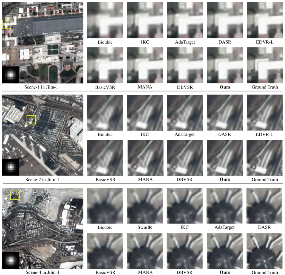
Figure 4: Qualitative results on Scene-1, Scene-2 and Scene-4 from Jilin-1 testset with various blur kernels. The size of the Region Of Interest (ROI) is $70\times 70$. Our method recovers more sharp and clean details than state-of-the-art non-blind and blind SR methods.

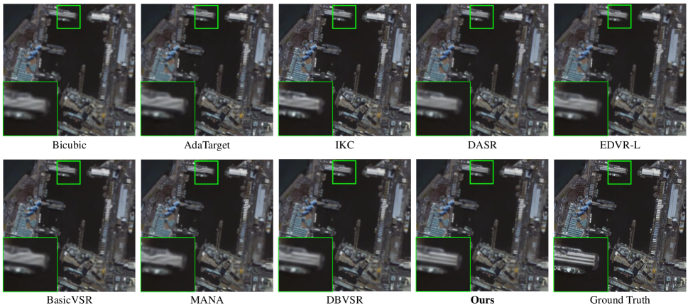
Figure 5: Qualitative results on UrtheCast test set with blur kernel width $\sigma=1.6$. The size of the Region Of Interest (ROI) is $90\times 90$. Our method has fewer distortions and restores more textures than other state-of-the-art non-blind and blind SR methods.

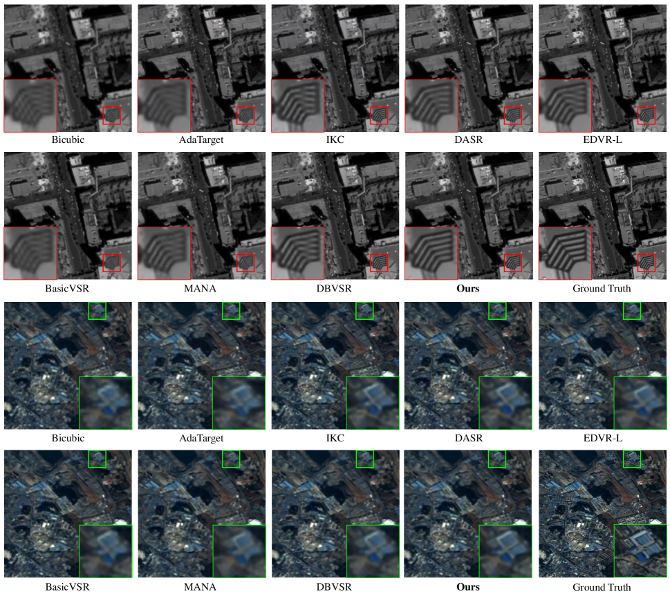
Figure 6: Qualitative results on SkySat-1 (top) and Zhuhai-1 (bottom) testsets with blur kernel width $\sigma=2.0$. The size of the Region Of Interest (ROI) is $70\times 70$. Our method produces more realistic and sharp details than state-of-the-art non-blind and blind SR methods.

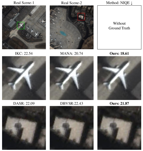
Figure 7: Real-world comparisons on Scene-1 and Scene-2 from Carbonite-2. Our method gains less blur on the boundary of the plane and building. A low NIQE represents a higher perceptual quality.

TABLE III: Quantitative results on the Carbonite-2 and UrtheCast testsets. Here, the PSNR/SSIM is the average result of all scenes on each test set. The best PSNR/SSIM performances are highlighted in bold red color, and the second-best results are marked in blue color. Note that BasicVSR is a recurrent method, and we followed the official settings, using 15 consecutive frames for propagation.

Methods	Input Frames	Publication	Carbonite-2			UrtheCast
			$\sigma=1.2$	$\sigma=1.6$	$\sigma=2.0$	$\sigma=1.2$	$\sigma=1.6$	$\sigma=2.0$
Bicubic	-	-	29.97/0.8445	30.04/0.8440	29.96/0.8395	25.77/0.7374	25.80/0.7315	25.70/0.7211
SwinIR [33]	Single	ICCV’21	30.74/0.8575	30.29/0.8484	30.29/0.8484	26.37/0.7589	26.09/0.7465	25.78/0.7328
IKC [47]	Single	CVPR’19	36.97/0.9353	36.74/0.9327	36.48/0.9286	29.98/0.8573	29.72/0.8427	29.65/0.8408
AdaTarget [49]	Single	CVPR’21	32.17/0.8849	32.11/0.8861	31.90/0.8842	24.76/0.6900	24.90/0.6940	25.00/0.6960
DASR [48]	Single	CVPR’21	36.91/0.9358	36.36/0.9304	35.86/0.9245	29.84/0.8527	29.81/0.8408	29.54/0.8343
DUF-52L [38]	7	CVPR’18	32.00/0.8855	31.46/0.8769	31.05/0.8663	26.61/0.7661	26.32/0.7483	26.13/0.7348
EDVR-L [40]	5	CVPRW’19	31.10/0.8635	32.07/0.8769	32.93/0.8898	24.87/0.7116	25.69/0.7444	26.55/0.7744
BasicVSR [73]	Recurrent	CVPR’21	33.62/0.9043	33.25/0.8983	32.63/0.8880	28.25/0.8212	28.08/0.8142	27.78/0.8055
MSDTGP [28]	5	TGRS’22	29.17/0.8252	29.08/0.8264	28.88/0.8227	26.59/0.7564	26.34/0.7408	25.82/0.7214
MANA [42]	7	CVPR’22	34.27/0.9174	33.42/0.9082	32.54/0.8946	25.72/0.7581	25.54/0.7475	25.48/0.7427
DBVSR [68]	5	ICCV’21	35.91/0.9280	35.92/0.9277	36.15/0.9289	29.64/0.8438	29.41/0.8351	29.02/0.8243
BSVSR (ours)	5	-	36.78/0.9359	37.05/0.9378	37.47/0.9401	29.90/0.8545	29.96/0.8500	29.94/0.8453

TABLE IV: Quantitative results on the SkySat-1 and Zhuhai-1 testsets. The best PSNR/SSIM performances are highlighted in bold red color, and the second-best results are marked in blue color.

Test Set	$\sigma$	Bicubic	IKC [47]	DASR [48]	EDVR-L [40]	BasicVSR [73]	MANA [42]	DBVSR [68]	BSVSR (ours)
SkySat-1	1.2	25.46/0.7573	31.36/0.8949	31.81/0.9054	27.33/0.8375	29.87/0.8723	29.72/0.8841	31.63/0.9085	31.77/0.9114
	1.6	25.50/0.7524	31.11/0.8897	31.53/0.8997	28.40/0.8593	29.75/0.8664	29.19/0.8735	31.82/0.9087	31.97/0.9125
	2.0	25.40/0.7417	30.84/0.8831	31.29/0.8940	29.43/0.8746	29.13/0.8492	28.75/0.8600	31.68/0.9041	32.06/0.9121
Zhuhai-1	1.2	24.98/0.6390	28.06/0.7526	27.91/0.7501	25.03/0.6461	27.12/0.7242	25.74/0.6838	27.72/0.7468	27.79/0.7509
	1.6	25.02/0.6300	27.59/0.7335	27.45/0.7298	25.20/0.6493	27.02/0.7136	25.37/0.6624	27.37/0.7235	27.73/0.7338
	2.0	24.93/0.6160	27.43/0.7275	27.26/0.7169	25.92/0.6764	26.87/0.7036	25.03/0.6437	27.52/0.7291	27.70/0.7311

IV Experiment and Discussion

IV-A Satellite Video Data source

To evaluate the performance of our BSVSR against state-of-the-art approaches, we conduct comprehensive experiments on five mainstream video satellites, including Jilin-1, Carbonite-2, UrtheCast, SkySat-1, and Zhuhai-1. The training set is cropped from Jilin-1 satellite videos, where the spatial resolution of the ground-truth video is $640\times 640$. Based on Equation 1, we degraded the high-resolution videos to generate low-resolution counterparts to establish the high-resolution and low-resolution training pairs. Following our previous works [28, 64], we ultimately obtained 189 video clips for model training. As for model testing, we randomly cropped 6 scenes from Jilin-1 that are non-overlapping with the training set. In addition, all the video clips of Carbonite-2, UrtheCast, SkySat-1, and Zhuhai-1 are used for further testing. The number of test video clips is 10, 14, 6, and 3. In the end, we had 39 videos from five video satellites for comprehensive model evaluation. A detailed summary of these five satellite videos can be found in Table I. Our dataset is publicly available at https://github.com/XY-boy.

IV-B Implementation Details

We set $s=4$ to focus on $\times 4$ blind SR for satellite video. As shown in Fig. 1, our network receives $2N+1=5$ consecutive frames as input, and the residual blocks extract homogeneous features with $C=128$ channels. For profound blur-aware transformation, we stack $n=20$ transformation module ${\rm{{\cal N}}}_{n}^{T}$, which strikes a balance between model size and performance. Consistent with previous blind VSR settings, we adopt isotropic Gaussian blur kernel of size $13\times 13$ to degrade the ground-truth videos, as isotropic Gaussian blur kernel is highly consistent with the blur distribution in satellite videos[26]. The standard deviation of Gaussian blur kernel is set to $\sigma\sim\left[{0.4,2}\right]$

During modeling training, we firstly sample 32 blurry LR video patches with a size of $64\times 64$ in each mini-batch to train ${{\rm{{\cal N}}}_{k}}$ by optimizing ${{\rm{{\cal L}}}_{kernel}}$ with a learning rate of $1\times 10^{-4}$. Subsequently, we train the entire model using the overall loss ${\rm{{\cal L}}}={{\rm{{\cal L}}}_{kernel}}+{{\rm{{\cal L}}}_{SR}}$, where ${{\rm{{\cal L}}}_{SR}}$ is the pixel-wise difference ${{\rm{{\cal L}}}_{SR}}={\left\|{I_{t}^{GT}-{I_{t}}^{SR}}\right\|_{1}}$ between restored mid-frame $I^{SR}_{t}$ and ground-truth $I^{GT}_{t}$ and $\rm{{\cal L}}_{kernel}$ is shown in Fig. 2(a). The learning rate is initialized to $1\times 10^{-4}$ and halved for every 25 epochs, and finally, our BSVSR model will reach convergence after 50 epochs. Date augmentation [74] is performed by random flipping and 90° rotation. We use the Adam optimizer for model optimization, and all experiments are conducted on a single NVIDIA RTX 3090 GPU with 24GB memory under the PyTorch framework.

IV-C Comparison With State-of-the-Arts

In this subsection, we comprehensively evaluate the effectiveness of our proposed BSVSR on synthetic and real-world satellite videos and compare it with state-of-the-art approaches. Both quantitative and qualitative results are presented and analyzed in detail.

IV-C1 Selected Methods and Metrics

The comparative approaches can be categorized into four types:

1. non-blind SISR model, as SwinIR [33];

2. blind SISR methods, including IKC [47], AdaTarget [49] and DASR [48];

3. non-blind VSR networks, such as DUF-52L [38], EDVR-L [40], BasicVSR [73], MSDTGP [28] and MANA [42];

4. blind VSR approach DBVSR [68].

In particular, for blind SISR: IKC estimate the explicit blur kernels and transforms the blur information with affine transformation, termed Spatial Feature Transformation (SFT) layer. Now, the SFT layer is prevailing in blind SISR models; DASR predicts the degradation representation without kernel correction, which is more efficient than IKC. Besides, a Degradation-aware Convolution (DAConv) is proposed in DASR for effective blur transformation; AdaTarget is an implicit blur transformation model which does not require blur estimation. Therefore, we include these representative blind SISR methods for comparison. For non-blind VSR: DUF-52L implicitly realizes temporal compensation using 3D dynamic filters; EDVR-L and MSDTGP employ deformable convolution to explore temporal priors. Notably, MSDTGP is specialized for satellite videos; BasicVSR is a bi-directional propagation approach that provides leading performance with optical flow compensation; MANA relies on non-local attention for compensation. Hence, these methods provide comprehensive coverage of mainstream temporal compensation strategies. As for blind VSR, few studies are available for comparison. DBVSR combines optical flow warping and SFT layer to achieve blind VSR, which produces promising results against non-blind models.

Three metrics are involved in the quantitative evaluation. In experiments on simulated data, the classical image quality indicator Peak Signal-to-Noise Ratio (PSNR) and Structural Similarity Index Measure (SSIM) are used to measure the fidelity between restored results and ground truth. In real-world experiments, the reference-free metric Natural Image Quality Evaluator (NIQE) [75] is adopted. NIQE compares the restored image to a default model computed from images of natural scenes. Note that a lower NIQE value indicates better quality of human perception.

IV-C2 Quantitative Comparison

Ascribing to the vital implementation of pixel-wise blur level measurement, our BSVSR is more flexible and allows accurate temporal compensation in blurry LR satellite videos. As reported in Table. II, III and IV, BSVSR achieves the best average performances on all test sets and is well-generalized in various blur kernels with kernel width $\sigma=1.2,1.6,2.0$.

For instance, when $\sigma=2.0$ on Jilin-1 testset in Table. II, our BSVSR gains a PSNR improvement of 4.21dB and 2.28dB compared to the best non-blind models SwinIR and EDVR-L, respectively. This illustrates that the classical SR approach is not capable of handling blind degradation processes, such as unknown blurs and downsampling. Compared to the best blind SISR method DASR, we can lead it by a large margin of 1.31dB, indicating that accurate temporal compensation is crucial for blind satellite VSR as it provides cleaner and sharper temporal cues to make the highly ill-posed problem well-posed. Although BSVSR shares the same blur estimation network with DBVSR, we can surpass it by 0.86dB, which demonstrates that temporal compensation also plays an important role in blind VSR. As mentioned before, most blind SR methods focus on blur estimation and overlook the critical aspect: temporal compensation. Under the same blur estimation procedure, the proposed progressive compensation strategy can extract more vital sharpness than the optical flow used in DBVSR, thus eliminating the interference of blurry pixels for better restoration.

Furthermore, as listed in Table III and IV, we found that the blind SISR methods without temporal compensation can outperform the blind VSR approaches, such as IKC can ahead DBVSR 0.34dB in UrtheCast when $\sigma=1.2$. On the one hand, this illustrates that temporal compensation in severely blurred and downsampled videos remains a challenging task because instead of exploring more complementary, inaccurate temporal compensation may introduce interference that is harmful to restoration. On the other hand, we can alleviate this misalignment by performing pixel-wise blur-level modeling with deformable attention.

IV-C3 Qualitative Comparison

The visual comparison results are shown in Fig. 4, 5, and 6, the proposed method is capable of recovering more sharp and reliable details in various blurs and scenes.

For example, as shown in Fig. 4, we observed that IKC and DBVSR restore apparent artifacts in Scene-2 of Jilin-1. This could be attributed to the mismatch between the estimated blur kernel or undesirable feature adaptation. Notably, the proposed BSVSR shares the same blur estimation component with DBVSR. However, it achieves favorable visual results, suggesting that the issue may not lie in the blur estimation but in the inaccurate blur transformation involved in DBVSR. Therefore, we can conclude that our pyramid spatial transformation can better calibrate the mid-feature to the correct solution space compared to SFT.

In Fig. 5, AdaTarget, IKC, BasicVSR, and MANA generate severe line distortion and blending, which completely deviate from the ground truth. Our BSVSR reconstructs the spatial details and structures better than DBVSR, which illustrates deformable attention success in exploring more sharp details from blurred LR frames than inaccurate optical flow warping. Similarly, as shown in Fig. 6, all of the comparative methods tend to recover more bent shapes and fuzzy edges of the buildings on the ground. Our BSVSR produces higher fidelity with reliable and sharp distributions against other non-blind and blind SR approaches.

IV-C4 Real-world Comparison

Apart from the experiments on simulated degradation, we further evaluate our method against state-of-the-art models on real-world satellite videos. The visual comparisons and corresponding NIQE metrics are shown in Fig. 7. Apparently, our method achieves the best NIQE, indicating the best human perception. Visually, IKC restores blur and noise on the edge of the plane, MANA creates unpleasing distortion in the tail, and our results are more clean and sharp in the high-frequency details.

IV-D Ablation Studies

In this section, we investigate the effectiveness of the key components of our BSVSR. Also, hyper-parameter setting and model efficiency are carefully discussed.

IV-D1 Effectiveness of Blur Kernel Estimation

To examine the effects of blur kernel estimation, we build three models for comparison: a) Model-1: we remove the network ${{\rm{{\cal N}}}_{k}}$, ${{\rm{{\cal N}}}_{FFT}}$ and ${{\rm{{\cal N}}}_{s}}$. In this case, we pass $I^{LR}_{t}$ to five $3\times 3$ convolution layers to generate ${\rm{{\cal F}}}_{t}^{s}$ for transformation; b) Model-2: we delete ${{\rm{{\cal N}}}_{k}}$ and do not estimate blur kernel $\rm{B_{t}}$. Here, we use bilinear upsampling to generate the latent sharp frame $I^{sharp}$; c) Model-3: we retain ${{\rm{{\cal N}}}_{k}}$ but do not optimize it with ${{\rm{{\cal L}}}_{kernel}}$. As reported in Table. V, Model-1 gets the worse performance as bilinear upsampling could not incorporate the blur information for blur-aware transformation. Model-2 could find some sharp cues with the help of sharp features extraction network. However, without the guidance of $\rm{B_{t}}$, it is hard to adjust the solution space to an accurate domain. Although Model-3 performs blur kernel estimation, it can not find the accurate blur distribution without the ${{\rm{{\cal L}}}_{kernel}}$. By applying the entire blur estimation process, our method gains substantial improvements for blind VSR tasks, such as leading Model-2 and Model-3 by 0.28dB and 3.8dB in terms of PSNR, respectively.

TABLE V: Ablation studies of blur kernel estimation. The PSNR (dB) is calculated in Scene-2 of Jinlin-T with $\sigma=1.6$.

Method	Model-1	Model-2 (w/o ${{\mathop{\rm B}\nolimits}_{t}}$)	Model-3 (w/o ${{\rm{{\cal L}}}_{kernel}}$)	Ours
PSNR	31.58	31.47	27.95	31.75
SSIM	0.9332	0.9278	0.8890	0.9361

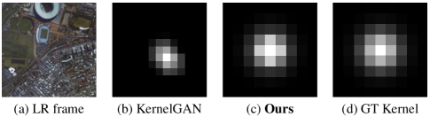
Figure 8: Visualization of estimated blur kernels. (a) Blurry low-resolution frame; (b) The estimated blur kernel of KernelGAN [76]; (c) The estimated blur kernel of our BSVSR. (d) The ground-truth blur kernel.

TABLE VI: Quantitative discussion of the progressive temporal compensation. One-stage means we directly align and fuse the $2N$ adjacent frames to the min-frame for temporal compensation. The PSNR (dB) is calculated in Scene-2 of Jinlin-T with $\sigma=1.6$.

Fusion strategy	Models	Flow	MSD	DA	PSNR (dB)
One-stage	Model-4	$\checkmark$			31.44
	Model-5		$\checkmark$		31.61
	Model-6			$\checkmark$	31.68
Progressive	Ours		$\checkmark$	$\checkmark$	31.75

Furthermore, as illustrated in Fig. 8, we visualize the estimated blur kernel $\rm{B_{t}}$ and compare it with another state-of-the-art blur kernel estimation approach KernelGAN [76]. Our estimated blur kernel is consistent with the ground-truth kernel, which illustrates that our model predicts the precise blur information from satellite videos to make the network better aware of the degradation process.

IV-D2 Effectiveness of Progressive Temporal Compensation

As mentioned before, since the optical flow estimation is laborious and inaccurate to describe the motion relationship in severely blurry and low-resolution satellite videos, we introduce the Multi-Scale Deformable (MSD) convolution and Deformable Attention (DA) to progressively aggregate more clean and sharp cues in a coarse-to-fine manner.

To begin with, we set up three baselines that directly align and fuse the blurry LR frames to generate the sharp mid-feature ${{\rm{\tilde{\cal F}}}_{t}}$ in a one-stage manner. Specifically, model-4 employs PWC-Net to estimate the optical flow maps from mid-frame $I^{LR}_{t}$ to adjacent frames. Then the warped adjacent features are concatenated and fused to ${{\rm{\tilde{\cal F}}}_{t}}$. Model-5 adopt MSD to align adjacent feature to min-feature, and the aligned features are concatenated and fused. Model-6 exploit DA to aggregate the frames. As listed in Table. VI, we find that progressive compensation shows more promising performance than one-stage compensation. As examined in previous works [77, 28], dividing the entire frame sequences into sub-sequence helps to alleviate the alignment difficulties caused by large-displacement. Our method uses a slid-window strategy to progressively merge the temporal information in each window, relieving the pressure of MSD alignment. Besides, the optical-flow-based compensation model produces the worse results in one-stage compensation models. Therefore, we argue that optical flows in not robust and accurate in blurry LR satellite videos.

In addition, we set different combinations in the coarse-to-fine compensation process. The results are reported in Table. VII, which indicates that MSD is more practical to explore coarse sharpness and DA can aggregate the final sharp mid-features by considering the blur level of pixels.

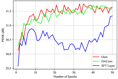
Figure 9: The training process of different transformation modules. Our Pyramid Spatial Transformation (PST) provides a more robust and effective blur transformation performance.

TABLE VII: Quantitative discussion of the coarse-to-fine temporal compensation. Model-7 to Model-11 adopt a different combination of fusion modules. The PSNR (dB) is calculated in Scene-2 of Jinlin-1 with $\sigma=1.6$.

Model	Fusion-1 (Coarse)	Fusion-2 (Fine)	PSNR (dB)
Model-7	Flow Warp + Conv	${{\rm{{\cal N}}}_{MSD}}$	31.58
Model-8	Flow Warp + Conv	${{\rm{{\cal N}}}_{DA}}$	31.65
Model-9	${{\rm{{\cal N}}}_{DA}}$	${{\rm{{\cal N}}}_{MSD}}$	31.69
Model-10	${{\rm{{\cal N}}}_{DA}}$	Flow Warp + Conv	31.54
Model-11	${{\rm{{\cal N}}}_{MSD}}$	Flow Warp + Conv	31.42
Ours	${{\rm{{\cal N}}}_{MSD}}$	${{\rm{{\cal N}}}_{DA}}$	31.75

TABLE VIII: Ablation analysis on the effectiveness of Pyramid Spatial Transformation (PST). Baseline means we replace PST with three convolution layers. SFT and DA Conv are two widely used blur transformation approaches. The PSNR (dB) is calculated in Scene-2 of Jinlin-1 with $\sigma=1.6$.

Model	Baseline	SFT Layer[47]	DA Conv [48]	PST (ours)
PSNR	31.21	31.33	31.69	31.75
SSIM	0.9287	0.9308	0.9345	0.9361

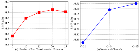
Figure 10: The impact of different hyper-parameters on the performance of our BSVSR.

TABLE IX: Quantitative comparisons of our method and SOTAs in terms of parameters, FLOPs, and running times. The FLOPs are calculated on 5 LR input frames with the size of $150\times 150$. The running time (f/ps) is the average inference consumption per frame. Note that 1M=$10^{6}$ and 1G=$10^{9}$. Here, the PSNR (dB) is the average test result on five satellite videos.

Methods	#Param (M)	FLOPs (G)	Time (s)	PSNR (dB)
SwinIR [33]	11.8	266.8	0.054	28.50
IKC [47]	9.5	130.6	0.045	31.78
AdaTarget [49]	16.7	403.4	0.137	28.56
DASR [48]	5.6	107.2	0.022	32.12
DUF-52L [38]	6.8	736.6	0.078	28.31
EDVR-L [40]	20.7	897.8	0.041	30.57
BasicVSR [73]	6.3	163.7	0.034	29.58
MSDTGP [28]	14.1	1579.8	0.128	29.87
MANA [42]	22.2	633.5	0.056	29.32
DBVSR [68]	14.1	1792.3	0.154	32.20
BSVSR (ours)	15.2	688.9	0.077	32.95

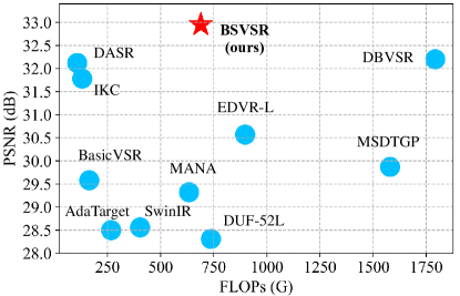
Figure 11: The relationship between FLOPs (G) and PSNR (dB) performance. Our BSVSR achieves a favorable trade-off between computational complexity and performance.

IV-D3 Effectiveness of Pyramid Spatial Transformation

With the awareness of blur information, we perform flexible transform to adjust the mid-feature in the spatial and channel dimension to make it adaptive to various degradations. To evaluate the proposed Pyramid Spatial Transformation (PST), we set a baseline model by replacing PST with three convolution layers. In addition, two widely used blur transformation modules, Spatial Feature Transformation (SFT) layer and Degradation-Aware Convolution (DAConv), are introduced as alternative transformation networks for comparison. The training process is displayed in Fig. 9, and the quantitative results can be found in Table. VIII. We observe that the SFT layer suffers instability in the training process. Benefiting from the well-defined spatial and channel activation, our method reflects robust blur transformation. Moreover, our PST ahead SFT layer and DA Conv of PNSR by 0.42dB and 0.06dB, respectively. As mentioned before, the pyramid structure is beneficial for preserving the multi-scale information in satellite videos. Therefore, we could conduct multi-level transformation to ensure more precise feature adaptation.

IV-D4 Model Efficiency

Here we firstly discuss the relationship between model size and performance of BSVSR by stacking different numbers $n$ of transformation network ${{\rm{{\cal N}}}_{n}^{T}}$. The quantitative of PSNR is provided in Fig. 10 (a). With the growing number of $n$, the communication between blur information and min-feature deepens, leading to better feature adaptation. However, such improvement reaches a plateau when $n=15$. Additionally, we investigate the impact of channel number $C$. As shown in Fig. 10 (b), despite increasing performance as $C$ grows, the huge parameters of our model become an urgent issue when $C$ is larger than 64. To achieve a favorable trade-off between model efficiency and performance, we adopt $n=20$ and $C=128$ in our final model.

Furthermore, we evaluate the model efficiency of comparative state-of-the-art methods in terms of parameters, FLOating Point operations (FLOPs), and running times. As reported in Table. IX, BSVSR gains the best performance with an acceptable model size. Note that SISR methods naturally have fewer parameters and FLOPs than the VSR approach as they do not include extra components for temporal compensation. Compared to the best non-blind VSR model EDVR-L, BSVSR is 27% less in parameters (15.2M vs. 20.7M) and 208.9 less in FLOPs. Regarding the blind VSR approach DBVSR, our BSVSR has significantly lower complexities (688.9G vs. 1792.3G) and faster inference speed (0.077s vs. 0.154s). This is because the optical flow estimation used in DBVSR is time-consuming, whereas our progressive compensation strategy is more computationally efficient and effective in temporal compensation. Fig. 11 gives a visual relationship between model performance and FLOPs. It is evident that our method achieved favorable performance compared to other methods while maintaining affordable complexity.

V Conclusion

In this paper, we proposed a blind SR network for satellite videos (BSVSR). Our key motivation is that not all the pixels can provide clean and sharp cues for blind VSR. Therefore, our BSVSR mainly aims at compensating for blurry and smooth pixels from severely degraded satellite videos by considering the blur level of pixels. Unlike prior blind satellite VSR methods that employ optical flow warping or patch-wise similarity to align frames, we progressively explore temporal redundancy using Multi-Scale Deformable (MSD) convolution and further aggregate them into a sharp mid-feature with multi-scale Deformable Attention (DA) in a coarse-to-fine manner. Additionally, we devise a robust pyramid spatial transformation module, which recalibrates the sharp mid-feature in the multi-level domain to modulate the mid-feature into a suitable solution space. Extensive experiments on five video satellites demonstrate our BSVSR gains favorable performance against state-of-the-art non-blind and blind SR approaches.

Although the proposed BSVSR could explore vital sharpness from blurry LR satellite videos, it still remains a challenging task to grasp beneficial information in compressed satellite imagery. Besides, missing a real-world satellite video dataset poses a domain gap between simulation and reality. In our future work, we plan to take the noise term into consideration and build a large-scale dataset with real-world degradations.

Yi Xiao received the B.S. degree from the School of Mathematics and Physics, China University of Geosciences, Wuhan, China, in 2020. He is pursuing the Ph.D. degree with the School of Geodesy and Geomatics, Wuhan University, Wuhan. His major research interests are remote sensing image super-resolution and computer vision. More details can be found at https://xy-boy.github.io.

Qiangqiang Yuan (Member, IEEE) received the B.S. degree in surveying and mapping engineering and the Ph.D. degree in photogrammetry and remote sensing from Wuhan University, Wuhan, China, in 2006 and 2012, respectively. In 2012, he joined the School of Geodesy and Geomatics, Wuhan University, where he is a Professor. He has published more than 90 research papers, including more than 70 peer-reviewed articles in international journals, such as Remote Sensing of Environment, ISPRS Journal of Photogrammetry and Remote Sensing, IEEE Transaction ON Image Processing, and IEEE Transactions ON Geoscience AND Remote Sensing. His research interests include image reconstruction, remote sensing image processing and application, and data fusion. Dr. Yuan was a recipient of the Youth Talent Support Program of China in 2019, the Top-Ten Academic Star of Wuhan University in 2011, and the recognition of Best Reviewers of the IEEE GRSL in 2019. In 2014, he received the Hong Kong Scholar Award from the Society of Hong Kong Scholars and the China National Postdoctoral Council. He is an associate editor of 5 international journals and has frequently served as a referee for more than 40 international journals for remote sensing and image processing.

Qiang Zhang received the B.E. degree in surveying and mapping engineering, M.E. and Ph.D. degree in photogrammetry and remote sensing from Wuhan University, Wuhan, China, in 2017, 2019 and 2022, respectively. He is currently an Associate Professor with the Center of Hyperspectral Imaging in Remote Sensing (CHIRS), Information Science and Technology College, Dalian Maritime University. His research interests include remote sensing information processing, computer vision, and machine learning. He has published more than ten journal papers on IEEE TIP, IEEE TGRS, ESSD, and ISPRS P&RS. More details could be found at https://qzhang95.github.io.

Liangpei Zhang (Fellow, IEEE) received the B.S. degree in physics from Hunan Normal University, Changsha, China, in 1982, the M.S. degree in optics from the Xi’an Institute of Optics and Precision Mechanics, Chinese Academy of Sciences, Xi’an, China, in 1988, and the Ph.D. degree in photogrammetry and remote sensing from Wuhan University, Wuhan, China, in 1998. He is currently a “Chang-Jiang Scholar” Chair Professor appointed by the Ministry of Education of China at the State Key Laboratory of Information Engineering in Surveying, Mapping, and Remote Sensing (LIESMARS), Wuhan University. He was a Principal Scientist for the China State Key Basic Research Project from 2011 to 2016 appointed by the Ministry of National Science and Technology of China to lead the Remote Sensing Program in China. He has published more than 700 research articles and five books. He is the Institute for Scientific Information (ISI) Highly Cited Author. He holds 30 patents. His research interests include hyperspectral remote sensing, high-resolution remote sensing, image processing, and artificial intelligence. Dr. Zhang is a fellow of the Institution of Engineering and Technology (IET). He was a recipient of the 2010 Best Paper Boeing Award, the 2013 Best Paper ERDAS Award from the American Society of Photogrammetry and Remote Sensing (ASPRS), and the 2016 Best Paper Theoretical Innovation Award from the International Society for Optics and Photonics (SPIE). His research teams won the top three prizes in the IEEE GRSS 2014 Data Fusion Contest. His students have been selected as the winners or finalists of the IEEE International Geoscience and Remote Sensing Symposium (IGARSS) Student Paper Contest in recent years. He is also the Founding Chair of the IEEE Geoscience and Remote Sensing Society (GRSS) Wuhan Chapter. He also serves as an associate editor or editor for more than ten international journals. He is also serving as an Associate Editor for the IEEE Transactions ON Geoscience AND Remote Sensing.

References

- [1] Q. Zhang, Q. Yuan, Z. Li, F. Sun, and L. Zhang, “Combined deep prior with low-rank tensor SVD for thick cloud removal in multitemporal images,” ISPRS J. Photogramm. Remote Sens., vol. 177, pp. 161–173, Jul. 2021.
- [2] M. Zhao, S. Li, S. Xuan, L. Kou, S. Gong, and Z. Zhou, “Satsot: A benchmark dataset for satellite video single object tracking,” IEEE Transactions on Geoscience and Remote Sensing, vol. 60, pp. 1–11, 2022.
- [3] T. Guo, L. He, F. Luo, X. Gong, Y. Li, and L. Zhang, “Anomaly detection of hyperspectral image with hierarchical anti-noise mutual-incoherence-induced low-rank representation,” IEEE Transactions on Geoscience and Remote Sensing, 2023.
- [4] Y. Xu, L. Zhang, B. Du, and L. Zhang, “Hyperspectral anomaly detection based on machine learning: An overview,” IEEE Journal of Selected Topics in Applied Earth Observations and Remote Sensing, vol. 15, pp. 3351–3364, 2022.
- [5] D. He and Y. Zhong, “Deep hierarchical pyramid network with high- frequency -aware differential architecture for super-resolution mapping,” IEEE Transactions on Geoscience and Remote Sensing, vol. 61, pp. 1–15, 2023.
- [6] J. Xie, L. Fang, B. Zhang, J. Chanussot, and S. Li, “Super resolution guided deep network for land cover classification from remote sensing images,” IEEE Transactions on Geoscience and Remote Sensing, vol. 60, pp. 1–12, 2022.
- [7] S. Li, W. Song, L. Fang, Y. Chen, P. Ghamisi, and J. A. Benediktsson, “Deep learning for hyperspectral image classification: An overview,” IEEE Transactions on Geoscience and Remote Sensing, vol. 57, no. 9, pp. 6690–6709, 2019.
- [8] T. Wang, Y. Gu, and G. Gao, “Satellite video scene classification using low-rank sparse representation two-stream networks,” IEEE Transactions on Geoscience and Remote Sensing, vol. 60, pp. 1–12, 2022.
- [9] Y. Duan, F. Luo, M. Fu, Y. Niu, and X. Gong, “Classification via structure-preserved hypergraph convolution network for hyperspectral image,” IEEE Transactions on Geoscience and Remote Sensing, vol. 61, pp. 1–13, 2023.
- [10] D. He, Q. Shi, X. Liu, Y. Zhong, G. Xia, and L. Zhang, “Generating annual high resolution land cover products for 28 metropolises in china based on a deep super-resolution mapping network using landsat imagery,” GIScience & Remote Sensing, vol. 59, no. 1, pp. 2036–2067, 2022.
- [11] F. Luo, T. Zhou, J. Liu, T. Guo, X. Gong, and J. Ren, “Multiscale diff-changed feature fusion network for hyperspectral image change detection,” IEEE Transactions on Geoscience and Remote Sensing, vol. 61, pp. 1–13, 2023.
- [12] B. Arad, R. Timofte, R. Yahel, N. Morag, A. Bernat, Y. Cai, J. Lin, Z. Lin, H. Wang, Y. Zhang et al., “Ntire 2022 spectral recovery challenge and data set,” in Proceedings of the IEEE/CVF Conference on Computer Vision and Pattern Recognition, 2022, pp. 863–881.
- [13] Q. Yang, Q. Yuan, L. Yue, T. Li, H. Shen, and L. Zhang, “Mapping pm2. 5 concentration at a sub-km level resolution: A dual-scale retrieval approach,” ISPRS Journal of Photogrammetry and Remote Sensing, vol. 165, pp. 140–151, 2020.
- [14] K. Jiang, Z. Wang, P. Yi, T. Lu, J. Jiang, and Z. Xiong, “Dual-path deep fusion network for face image hallucination,” IEEE Transactions on Neural Networks and Learning Systems, vol. 33, no. 1, pp. 378–391, 2020.
- [15] Y. Xiao, Y. Wang, Q. Yuan, J. He, and L. Zhang, “Generating a long-term (2003- 2020) hourly 0.25° global pm2. 5 dataset via spatiotemporal downscaling of cams with deep learning (deepcams),” Science of The Total Environment, vol. 848, p. 157747, 2022.
- [16] J. He, Q. Yuan, J. Li, Y. Xiao, D. Liu, H. Shen, and L. Zhang, “Spectral super-resolution meets deep learning: Achievements and challenges,” Information Fusion, p. 101812, 2023.
- [17] F. Li, X. Jia, D. Fraser, and A. Lambert, “Super resolution for remote sensing images based on a universal hidden markov tree model,” IEEE Transactions on Geoscience and Remote Sensing, vol. 48, no. 3, pp. 1270–1278, 2010.
- [18] Y. Wang, Q. Yuan, T. Li, L. Zhu, and L. Zhang, “Estimating daily full-coverage near surface o3, co, and no2 concentrations at a high spatial resolution over china based on s5p-tropomi and geos-fp,” ISPRS Journal of Photogrammetry and Remote Sensing, vol. 175, pp. 311–325, 2021.
- [19] Y. Wang, Q. Yuan, L. Zhu, and L. Zhang, “Spatiotemporal estimation of hourly 2-km ground-level ozone over china based on himawari-8 using a self-adaptive geospatially local model,” Geoscience Frontiers, vol. 13, no. 1, p. 101286, 2022.
- [20] Z. Li, Q. Yuan, and L. Zhang, “Geo-intelligent retrieval framework based on machine learning in the cloud environment: A case study of soil moisture retrieval,” IEEE Transactions on Geoscience and Remote Sensing, pp. 1–1, 2023.
- [21] Q. Zhang, Y. Zheng, Q. Yuan, M. Song, H. Yu, and Y. Xiao, “Hyperspectral image denoising: From model-driven, data-driven, to model-data-driven,” IEEE Trans. Neural Netw. Learn. Syst., pp. 1–21, Jun. 2023.
- [22] F. Wang, J. Li, Q. Yuan, and L. Zhang, “Local–global feature-aware transformer based residual network for hyperspectral image denoising,” IEEE Transactions on Geoscience and Remote Sensing, vol. 60, pp. 1–19, 2022.
- [23] Q. Zhang, Q. Yuan, M. Song, H. Yu, and L. Zhang, “Cooperated spectral low-rankness prior and deep spatial prior for hsi unsupervised denoising,” IEEE Transactions on Image Processing, vol. 31, pp. 6356–6368, 2022.
- [24] K. Jiang, Z. Wang, P. Yi, G. Wang, K. Gu, and J. Jiang, “Atmfn: Adaptive-threshold-based multi-model fusion network for compressed face hallucination,” IEEE Transactions on Multimedia, vol. 22, no. 10, pp. 2734–2747, 2019.
- [25] K. Jiang, Z. Wang, P. Yi, C. Chen, Z. Wang, X. Wang, J. Jiang, and C.-W. Lin, “Rain-free and residue hand-in-hand: A progressive coupled network for real-time image deraining,” IEEE Transactions on Image Processing, vol. 30, pp. 7404–7418, 2021.
- [26] H. Liu and Y. Gu, “Deep joint estimation network for satellite video super-resolution with multiple degradations,” IEEE Transactions on Geoscience and Remote Sensing, vol. 60, pp. 1–15, 2022.
- [27] X. Zhu, W. Su, L. Lu, B. Li, X. Wang, and J. Dai, “Deformable detr: Deformable transformers for end-to-end object detection,” in International Conference on Learning Representations, 2021.
- [28] Y. Xiao, X. Su, Q. Yuan, D. Liu, H. Shen, and L. Zhang, “Satellite video super-resolution via multiscale deformable convolution alignment and temporal grouping projection,” IEEE Transactions on Geoscience and Remote Sensing, vol. 60, pp. 1–19, 2022.
- [29] C. Dong, C. C. Loy, K. He, and X. Tang, “Image super-resolution using deep convolutional networks,” IEEE Transactions on Pattern Analysis and Machine Intelligence, vol. 38, no. 2, pp. 295–307, 2016.
- [30] J. Kim, J. K. Lee, and K. M. Lee, “Accurate image super-resolution using very deep convolutional networks,” in Proceedings of the IEEE conference on computer vision and pattern recognition, 2016, pp. 1646–1654.
- [31] Y. Zhang, K. Li, K. Li, L. Wang, B. Zhong, and Y. Fu, “Image super-resolution using very deep residual channel attention networks,” in Proceedings of the European conference on computer vision (ECCV), 2018, pp. 286–301.
- [32] K. Jiang, Z. Wang, P. Yi, and J. Jiang, “Hierarchical dense recursive network for image super-resolution,” Pattern Recognition, vol. 107, p. 107475, 2020.
- [33] J. Liang, J. Cao, G. Sun, K. Zhang, L. Van Gool, and R. Timofte, “Swinir: Image restoration using swin transformer,” in Proceedings of the IEEE/CVF International Conference on Computer Vision, 2021, pp. 1833–1844.
- [34] J. He, Q. Yuan, J. Li, Y. Xiao, X. Liu, and Y. Zou, “Dster: A dense spectral transformer for remote sensing spectral super-resolution,” International Journal of Applied Earth Observation and Geoinformation, vol. 109, p. 102773, 2022.
- [35] A. Kappeler, S. Yoo, Q. Dai, and A. K. Katsaggelos, “Video super-resolution with convolutional neural networks,” IEEE transactions on computational imaging, vol. 2, no. 2, pp. 109–122, 2016.
- [36] J. Caballero, C. Ledig, A. Aitken, A. Acosta, J. Totz, Z. Wang, and W. Shi, “Real-time video super-resolution with spatio-temporal networks and motion compensation,” in Proceedings of the IEEE conference on computer vision and pattern recognition, 2017, pp. 4778–4787.
- [37] M. Haris, G. Shakhnarovich, and N. Ukita, “Recurrent back-projection network for video super-resolution,” in Proceedings of the IEEE/CVF Conference on Computer Vision and Pattern Recognition, 2019, pp. 3897–3906.
- [38] Y. Jo, S. W. Oh, J. Kang, and S. J. Kim, “Deep video super-resolution network using dynamic upsampling filters without explicit motion compensation,” in Proceedings of the IEEE conference on computer vision and pattern recognition, 2018, pp. 3224–3232.
- [39] Y. Tian, Y. Zhang, Y. Fu, and C. Xu, “Tdan: Temporally-deformable alignment network for video super-resolution,” in Proceedings of the IEEE/CVF Conference on Computer Vision and Pattern Recognition, 2020, pp. 3360–3369.
- [40] X. Wang, K. C. Chan, K. Yu, C. Dong, and C. Change Loy, “Edvr: Video restoration with enhanced deformable convolutional networks,” in Proceedings of the IEEE/CVF Conference on Computer Vision and Pattern Recognition Workshops, 2019, pp. 0–0.
- [41] H. Song, W. Xu, D. Liu, B. Liu, Q. Liu, and D. N. Metaxas, “Multi-stage feature fusion network for video super-resolution,” IEEE Transactions on Image Processing, vol. 30, pp. 2923–2934, 2021.
- [42] J. Yu, J. Liu, L. Bo, and T. Mei, “Memory-augmented non-local attention for video super-resolution,” in Proceedings of the IEEE/CVF Conference on Computer Vision and Pattern Recognition, 2022, pp. 17 834–17 843.
- [43] P. Yi, Z. Wang, K. Jiang, J. Jiang, T. Lu, X. Tian, and J. Ma, “Omniscient video super-resolution,” in Proceedings of the IEEE/CVF International Conference on Computer Vision, 2021, pp. 4429–4438.
- [44] K. C. Chan, S. Zhou, X. Xu, and C. C. Loy, “Basicvsr++: Improving video super-resolution with enhanced propagation and alignment,” in Proceedings of the IEEE/CVF Conference on Computer Vision and Pattern Recognition, 2022, pp. 5972–5981.
- [45] K. Zhang, W. Zuo, and L. Zhang, “Learning a single convolutional super-resolution network for multiple degradations,” in Proceedings of the IEEE Conference on Computer Vision and Pattern Recognition (CVPR), June 2018.
- [46] K. Zhang, L. V. Gool, and R. Timofte, “Deep unfolding network for image super-resolution,” in Proceedings of the IEEE/CVF Conference on Computer Vision and Pattern Recognition (CVPR), June 2020.
- [47] J. Gu, H. Lu, W. Zuo, and C. Dong, “Blind super-resolution with iterative kernel correction,” in Proceedings of the IEEE/CVF Conference on Computer Vision and Pattern Recognition, 2019, pp. 1604–1613.
- [48] L. Wang, Y. Wang, X. Dong, Q. Xu, J. Yang, W. An, and Y. Guo, “Unsupervised degradation representation learning for blind super-resolution,” in Proceedings of the IEEE/CVF Conference on Computer Vision and Pattern Recognition, 2021, pp. 10 581–10 590.
- [49] Y. Jo, S. W. Oh, P. Vajda, and S. J. Kim, “Tackling the ill-posedness of super-resolution through adaptive target generation,” in Proceedings of the IEEE/CVF Conference on Computer Vision and Pattern Recognition (CVPR), June 2021, pp. 16 236–16 245.
- [50] A. Bulat, J. Yang, and G. Tzimiropoulos, “To learn image super-resolution, use a gan to learn how to do image degradation first,” in Proceedings of the European Conference on Computer Vision (ECCV), September 2018.
- [51] M. Fritsche, S. Gu, and R. Timofte, “Frequency separation for real-world super-resolution,” in 2019 IEEE/CVF International Conference on Computer Vision Workshop (ICCVW), 2019, pp. 3599–3608.
- [52] Y. Yuan, S. Liu, J. Zhang, Y. Zhang, C. Dong, and L. Lin, “Unsupervised image super-resolution using cycle-in-cycle generative adversarial networks,” in Proceedings of the IEEE Conference on Computer Vision and Pattern Recognition (CVPR) Workshops, June 2018.
- [53] A. Liu, Y. Liu, J. Gu, Y. Qiao, and C. Dong, “Blind image super-resolution: A survey and beyond,” IEEE Transactions on Pattern Analysis and Machine Intelligence, vol. 45, no. 5, pp. 5461–5480, 2023.
- [54] H. Wu, N. Ni, and L. Zhang, “Lightweight stepless super-resolution of remote sensing images via saliency-aware dynamic routing strategy,” IEEE Transactions on Geoscience and Remote Sensing, 2023.
- [55] K. Jiang, Z. Wang, P. Yi, J. Jiang, J. Xiao, and Y. Yao, “Deep distillation recursive network for remote sensing imagery super-resolution,” Remote Sensing, vol. 10, no. 11, p. 1700, 2018.
- [56] S. Jia, Z. Wang, Q. Li, X. Jia, and M. Xu, “Multiattention generative adversarial network for remote sensing image super-resolution,” IEEE Transactions on Geoscience and Remote Sensing, vol. 60, pp. 1–15, 2022.
- [57] X. Dong, X. Sun, X. Jia, Z. Xi, L. Gao, and B. Zhang, “Remote sensing image super-resolution using novel dense-sampling networks,” IEEE Transactions on Geoscience and Remote Sensing, vol. 59, no. 2, pp. 1618–1633, 2021.
- [58] K. Jiang, Z. Wang, P. Yi, G. Wang, T. Lu, and J. Jiang, “Edge-enhanced gan for remote sensing image superresolution,” IEEE Transactions on Geoscience and Remote Sensing, vol. 57, no. 8, pp. 5799–5812, 2019.
- [59] Y. Xiao, X. Su, and Q. Yuan, “A recurrent refinement network for satellite video super-resolution,” in 2021 IEEE International Geoscience and Remote Sensing Symposium IGARSS. IEEE, 2021, pp. 3865–3868.
- [60] H. Liu, Y. Gu, T. Wang, and S. Li, “Satellite video super-resolution based on adaptively spatiotemporal neighbors and nonlocal similarity regularization,” IEEE Transactions on Geoscience and Remote Sensing, vol. 58, no. 12, pp. 8372–8383, 2020.
- [61] Z. He, J. Li, L. Liu, D. He, and M. Xiao, “Multiframe video satellite image super-resolution via attention-based residual learning,” IEEE Transactions on Geoscience and Remote Sensing, vol. 60, pp. 1–15, 2021.
- [62] Y. Xiao, Q. Yuan, J. He, Q. Zhang, J. Sun, X. Su, J. Wu, and L. Zhang, “Space-time super-resolution for satellite video: A joint framework based on multi-scale spatial-temporal transformer,” International Journal of Applied Earth Observation and Geoinformation, vol. 108, p. 102731, 2022.
- [63] X. Jin, J. He, Y. Xiao, and Q. Yuan, “Learning a local-global alignment network for satellite video super-resolution,” IEEE Geoscience and Remote Sensing Letters, 2023.
- [64] Y. Xiao, Q. Yuan, K. Jiang, X. Jin, J. He, L. Zhang, and C.-w. Lin, “Local-global temporal difference learning for satellite video super-resolution,” arXiv preprint arXiv:2304.04421, 2023.
- [65] Y. Xiao, Q. Yuan, K. Jiang, J. He, Y. Wang, and L. Zhang, “From degrade to upgrade: Learning a self-supervised degradation guided adaptive network for blind remote sensing image super-resolution,” Information Fusion, vol. 96, pp. 297–311, 2023.
- [66] H. Wu, N. Ni, S. Wang, and L. Zhang, “Blind super-resolution for remote sensing images via conditional stochastic normalizing flows,” arXiv preprint arXiv:2210.07751, 2022.
- [67] Z. He, D. He, X. Li, and R. Qu, “Blind superresolution of satellite videos by ghost module-based convolutional networks,” IEEE Transactions on Geoscience and Remote Sensing, vol. 61, pp. 1–19, 2023.
- [68] J. Pan, H. Bai, J. Dong, J. Zhang, and J. Tang, “Deep blind video super-resolution,” in Proceedings of the IEEE/CVF International Conference on Computer Vision, 2021, pp. 4811–4820.
- [69] D. Sun, X. Yang, M.-Y. Liu, and J. Kautz, “Pwc-net: Cnns for optical flow using pyramid, warping, and cost volume,” in Proceedings of the IEEE conference on computer vision and pattern recognition, 2018, pp. 8934–8943.
- [70] L. Fang, Y. Jiang, Y. Yan, J. Yue, and Y. Deng, “Hyperspectral image instance segmentation using spectral–spatial feature pyramid network,” IEEE Transactions on Geoscience and Remote Sensing, vol. 61, pp. 1–13, 2023.
- [71] J. Hu, L. Shen, and G. Sun, “Squeeze-and-excitation networks,” in Proceedings of the IEEE conference on computer vision and pattern recognition, 2018, pp. 7132–7141.
- [72] W. Shi, J. Caballero, F. Huszar, J. Totz, A. P. Aitken, R. Bishop, D. Rueckert, and Z. Wang, “Real-time single image and video super-resolution using an efficient sub-pixel convolutional neural network,” in Proceedings of the IEEE Conference on Computer Vision and Pattern Recognition (CVPR), June 2016.
- [73] K. C. Chan, X. Wang, K. Yu, C. Dong, and C. C. Loy, “Basicvsr: The search for essential components in video super-resolution and beyond,” in Proceedings of the IEEE/CVF Conference on Computer Vision and Pattern Recognition, 2021, pp. 4947–4956.
- [74] Q. Zhang, Q. Yuan, J. Li, Z. Li, H. Shen, and L. Zhang, “Thick cloud and cloud shadow removal in multitemporal imagery using progressively spatio-temporal patch group deep learning,” ISPRS J. Photogramm. Remote Sens., vol. 162, pp. 148–160, Apr. 2020.
- [75] A. Mittal, R. Soundararajan, and A. C. Bovik, “Making a “completely blind” image quality analyzer,” IEEE Signal Processing Letters, vol. 20, no. 3, pp. 209–212, 2013.
- [76] S. Bell-Kligler, A. Shocher, and M. Irani, “Blind super-resolution kernel estimation using an internal-gan,” in Advances in Neural Information Processing Systems, vol. 32, 2019.
- [77] T. Isobe, S. Li, X. Jia, S. Yuan, G. Slabaugh, C. Xu, Y.-L. Li, S. Wang, and Q. Tian, “Video super-resolution with temporal group attention,” in Proceedings of the IEEE/CVF conference on computer vision and pattern recognition, 2020, pp. 8008–8017.