Ultra-robust topologically protected edge states in quasi-1D systems

Abstract

Topological materials yield robust edge states with potential applications in electronics or quantum technologies. Yet, their simplest Su–Schrieffer–Heeger model covers only coupling disorders, leaving other types unexplored. Here, by studying a quasi-one-dimensional zigzag model with negative couplings, we show non-chiral edge states simultaneously resilient to dissipation, hopping and on-site energy disorders. To this end, we derive regularized values of the topological invariant via a novel approach. Our work hints on constructing topological phases even in the absence of usual symmetries.

Introduction.—Topologically protected one-dimensional edge states are quantum states of matter whose wave function is concentrated at the edges of a 1D lattice, and vanishes in its bulk. Lattice symmetries shield them from noise, crystal defects, or chemical composition changes [1, 2]. Their energy levels lie inside the energy gap between the valence and conduction bands. Beyond fundamental studies [3, 4, 5, 6, 7], they open prospects for fault-tolerant quantum computation [8, 9, 10, 11, 12], robust information processing [13, 14, 15, 16, 17, 18] and building numerous devices [19, 20, 21, 22, 23].

The best known edge states are protected by the chiral symmetry, described by the Su–Schrieffer–Heeger (SSH) chain model [24, 25, 26]. Here, an electron can either hop between the two sites within the unit cell, or to an adjoining one, with strengths $v$ and $w$, respectively. If $w>v$, topologically protected states appear.

Various models offering edge states have been proposed, including SSH generalizations [27, 28, 29, 30, 31], quasicrystal structures [32, 33, 34], the Aubry–André–Harper (AAH) model [35, 36], and Anderson topological insulators [37, 38]. They exhibit robustness against disorders in couplings that result from variations in distances between quantum particles [39, 40]. However, while the previous research addressed spectral disorders and on-site imperfections, particularly in non-dissipative systems [41, 42], the effects of site-dependent losses and phase disorder have received scant attention. These imperfections can significantly degrade edge state localization, induce energy gap closure, and prompt a shift from topological to conventional matter [1, 2]. Therefore, developing edge states resilient to these defects is crucial.

(a)
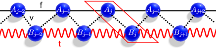
(b)

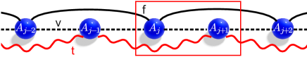
Figure 1: (a) Quasi-1D zigzag structure with interacting chains $A$ and $B$ connected by strength $v>0$ (dashed line). The coupling strengths between the sites within chain $A$ is $f>0$ (black line), while within $B$ is $t<0$ (red line). (b) Our system can be represented as a chain with next-neighbor and long-range interactions. An elementary two-site unit cell is shown as a red frame.

This letter presents the emergence of remarkably resilient topologically protected edge states in a quasi-1D zigzag structure where some lattice couplings are negative (with phase $\pi$), even in the absence of chiral symmetry. These states maintain their nature despite simultaneous disorders in lattice couplings, variations in on-site phases and potentials, and dissipation. Negative couplings play a crucial role in their concurrent stabilizing, enhancing localization, and controlling energy gaps. We introduce a novel approach to restore bulk-boundary correspondence, and to enable computing a regularized topological invariant. It establishes a continuous mapping between the original model and the “parental model”, with restored chiral symmetry. To this end, we construct in the Fourier space a special variant of the unit cell that we call “weighted”.

Negative couplings have gained attention for achieving non-trivial topological phases and creating energy gaps [43, 44, 45, 46, 47, 48, 49]. An example is the quadrupole topological insulator (QTI) exhibiting corner states limited by resistance to interaction strength disorders [43, 50]. Negative couplings naturally emerge in quantum particle interactions in alternative media: atoms in optical potentials [51, 52], arrays of microwave resonators [53, 50], optical waveguide lattices [54, 55, 56, 57, 44, 58, 59, 49], acoustic cavities [46, 60, 47], synthetic dimensions [61, 62], or resonant electric circuits [63, 64].

Our results pave the way for realistic implementation of topological quantum computing, information processing, and quantum transport on numerous platforms, including photonic, acoustic, mechanical metamaterials, and resonant electric circuits.

Edge states.—Let us consider the zigzag structure shown in Fig. 1a where one of the interaction strength is negative. It is composed of two interacting topologically trivial chains $A$ and $B$, and it is described by a finite tight-binding Hamiltonian

$$H\!=\!\!\!\sum_{j=1}^{N-1}\bigl{(}va_{j}^{\dagger}b_{j+1}+fa^{\dagger}_{j}a_{j+1}+tb^{\dagger}_{j}b_{j+1}\bigr{)}+\!\!\sum_{j=1}^{N}va^{\dagger}_{j}b_{j}+h.c.,$$ (1)

where $N$ is the number of sites on each chain, $v\geq 0$ is the hopping amplitude between them, $f\geq 0$ ($t\leq 0$) is the hopping amplitude within the chain $A$ ($B$); and $a_{j}$ ($a_{j}^{\dagger}$) and $b_{j}$ ($b_{j}^{\dagger}$) denote annihilation (creation) operators at the $j$-th site of the chain $A$ ($B$). Note that we did not made any assumption of the statistics that the operators $a$ and $b$ follow.

Our system can be viewed as a chain with uniform strength of next-neighbor (nn) interactions, and two opposite in phase strengths of next-next-neighbor (nnn) interactions, Fig. 1b. The presence of long-range repulsive and attractive interactions renders this model distinct from the SSH and AAH. All its non-trivial topological properties are due to the nnn-interactions; a model without them becomes a topologically trivial gapless chain. The analysis of energy bands of $H/f$ in terms of the inverse participation ratio $\mathfrak{I}$ (IPR) [65] (see Supplemental Material, SM, Section S1) for a chain of $90$ sites shown in Fig. 2a reveals the presence of two bands if $v^{2}>tf(t+1)^{2}(f+1)^{2}$ and $f\neq t$, and edge states within the gap if $v^{2}/4>tf$ and $v\neq 0$. The distance between the edge state and the closest band is larger, and the above inequalities always hold true simultaneously if $t/f<0$. Figs. 2b–c show the structure of edge states for $t=-f$, when the system acquires chiral symmetry.

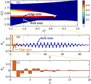
Figure 2: (a) Energy band structure of the zigzag system with $N=90$ sites computed for $v/f=1$, as a function of the interaction strengths’ ratio $t/f$. The edge (red) and bulk (blue) states here and further are highlighted using the inverse participation ratio (IPR) $\mathfrak{I}$. (b) Mode amplitude $\Psi_{k}$ on site $k$ of the edge and bulk states’ wave function evaluated for $t/f=-1$. (c) Profile of an edge state eigenmode shown for the first $20$ sites.

To describe the bulk properties of the two-band spectrum shown in Fig. 2, it is sufficient to consider a unit cell that consists of two sites, $A$ and $B$, and the corresponding bulk Hamiltonian in the continuum space

$$H_{2}(k_{x})=\begin{pmatrix}2f\cos{k_{x}}&v\bigl{(}1+e^{-ik_{x}}\bigr{)}\\ v\bigl{(}1+e^{ik_{x}}\bigr{)}&2t\cos{k_{x}}\end{pmatrix}.$$ (2)

Then, the bulk spectrum equals $\varepsilon=(f+t)\cos k_{x}\break\pm\sqrt{(f-t)^{2}\cos^{2}k_{x}+2v^{2}(1+\cos k_{x})}$. If $t=-f$, it exhibits the chiral symmetry, $\Gamma_{2}H_{2}(k_{x})\Gamma_{2}^{*}=-H_{2}(k_{x})$, where $\Gamma_{2}=\sigma_{y}T_{2}$, and the winding number is $W=0$ [66]. In a general case, however, the $2\times 2$ bulk model in Eq. (2) possesses neither chiral nor inversion symmetry. Thus, both the Zak phase and the winding number are not quantized, and the use of bulk-edge correspondence is not justified.

Topological invariant.—We propose to construct a “parental” model that features the chiral symmetry, connected to our original zigzag model by a continuous mapping, Fig. 3a. Here, this “parental” model is a ladder system, Fig. 3b, with initial setting $w=0$, coinciding with Fig. 1a for $w=v$. Since transition occurs without closing the energy gap, the two models can be continuously connected by a mapping $f(H_{4}):=(\Gamma_{4}H_{4}\Gamma_{4}^{*}-H_{4})/2$, where $\Gamma_{4}=\sigma_{z}\otimes I_{2}$ is the chiral symmetry operator for the “parental” model.

Let $H_{4}^{\text{par}}$ and $H_{4}^{\text{zig}}$ are the bulk Hamiltonians of the “parental” and the zigzag models, respectively, both defined on a four-site unit cell. Then, $f(H_{4}^{\text{par}})=f(H_{4}^{\text{zig}})=H_{4}^{\text{par}}$. This allows us to draw conclusions about topological edge states in the zigzag structure solely based on the analysis of the ladder system. The construction of the winding number for the latter requires a regularization step: the quasi-1D nature necessitates a correct geometrical interpretation of couplings $v$ (perpendicular to the selected momentum direction) between two chains.

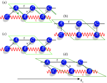
Figure 3: “Parental” model for the quasi-1D zigzag structure. (a) We generalize the zigzag model by allowing the chains $A$ and $B$ to interact with two alternating strengths, $v$ and $w$. For $f=t=0$ it restores the SSH model. (b) If $w=0$, the model amounts to a ladder with four-site non-trivial unit cell. (c) and (d) are two geometrical interpretations of the quasi-1D ladder structure. Unit cells at (b), (c) and (d) correspond to Hamiltonians $H_{4}\left(\raisebox{-0.25pt}{\includegraphics[width=11.9501pt]{Kachin_symbol3.pdf}}\right)$, $H_{4}\left(\raisebox{-0.25pt}{\includegraphics[width=11.9501pt]{Kachin_symbol2.pdf}}\right)$ and $H_{4}\left(\raisebox{-0.25pt}{\includegraphics[width=11.9501pt]{Kachin_symbol1.pdf}}\right)$, respectively.

Let us now denote the unit cells of the ladder systems from Fig. 3b–d as , , and , respectively. While Hamiltonian $H_{4}\left(\raisebox{-0.25pt}{\includegraphics[width=11.9501pt]{Kachin_symbol3.pdf}}\right)$ requires definition, the winding number integral calculated for Hamiltonians $H_{4}\left(\raisebox{-0.25pt}{\includegraphics[width=11.9501pt]{Kachin_symbol2.pdf}}\right)$ and $H_{4}\left(\raisebox{-0.25pt}{\includegraphics[width=11.9501pt]{Kachin_symbol1.pdf}}\right)$ yields $W=1$ in the presence of in-gap edge states, and does not converge in their absence. Thus, we construct a “weighted” unit cell, and the corresponding Hamiltonian $H_{4}\left(\raisebox{-0.25pt}{\includegraphics[width=11.9501pt]{Kachin_symbol3.pdf}}\right)$

$$H_{4}\left(\raisebox{-0.25pt}{\includegraphics[width=11.9501pt]{Kachin_symbol3.pdf}}\right)=\frac{H_{4}\left(\raisebox{-0.25pt}{\includegraphics[width=11.9501pt]{Kachin_symbol2.pdf}}\right)+\xi H_{4}\left(\raisebox{-0.25pt}{\includegraphics[width=11.9501pt]{Kachin_symbol1.pdf}}\right)}{\xi+1},$$ (3)

which properties in the basis of $\Gamma_{4}$ are determined by the upper-right block

$$h_{2}(k_{x},\xi)=\begin{pmatrix}f\bigl{(}1+e^{-ik_{x}}\bigr{)}&v\frac{e^{-ik_{x}}+\xi e^{ik_{x}}}{\xi+1}\\ v&t\bigl{(}1+e^{-ik_{x}}\bigr{)}\end{pmatrix}.$$ (4)

It also governs the winding number which takes the form

$$W={} \frac{1}{i2\pi}\int_{BZ}dk_{x}\textrm{Tr}\left(h_{2}(k_{x},\xi)^{-1}\frac{d}{dk_{x}}h_{2}(k_{x},\xi)\right)={}$$

$${}={} \int_{0}^{2\pi}\frac{dk_{x}}{2\pi}\frac{\frac{2ft}{v^{2}}(\xi+1)\left(1+e^{-ik_{x}}\right)+\left(\xi e^{2ik_{x}}-1\right)}{\frac{2ft}{v^{2}}(\xi+1)(1+\cos{k_{x}})-\left(\xi e^{2ik_{x}}+1\right)}.$$ (5)

For $\xi\ll 1$, the integral in $W$ does not converge. However, larger values of $\xi$ lead to the identification of non-trivial region, namely $W=1$ for $t\in(-\infty;v^{2}/(4f))$ and $W=0$ for $t\in[v^{2}/(4f);\infty)$.

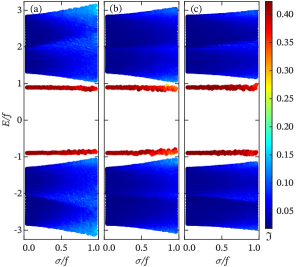
Figure 4: Energy eigenmodes computed for a chiral ($t/f=-1$) zigzag system with $N=90$ sites and $v/f=1$, averaged over 30 random instances of a disorder in (a) nn interactions, (b) nnn interactions, and (c) on-site energy, as a function of the disorder strength $\sigma/f$. The findings stem from analyzing the finite Hamiltonian $H_{\sigma}=H+\sigma D$, featuring the tight-binding Hamiltonian $H$ and the disorder operator $D$.

Robustness to disorders.—We explored the robustness of edge states in the zigzag system against disorders in the strengths of the nn and nnn interactions, and against the spectral disorder, by computing the energy spectrum of the Hamiltonian $H_{\sigma}=H+\sigma D$, where $H$ is defined by Eq. (1), $\sigma$ is a constant that quantifies the strength of the disorder, and $D$ is a matrix that defines the type of disorder. The matrix elements $D_{l,m}=\Delta d\delta_{l\pm 1,m}$ and $D_{l,m}=\Delta d\delta_{l\pm 2,m}$ represent the disorder in the nn and nnn coupling constants, while $D_{l,m}=\Delta d\delta_{l,m}$ model the spectral disorder. We sampled $\Delta d$ uniformly in range $[-0.5;0.5]$.

Fig. 4 depicts the spectrum of $H_{\sigma}$ computed for the chiral ($t/f=-1$) zigzag chain that was averaged over 30 random instances of a disorder in (a) next-neighbor, (b) long-range interactions, and (c) on-site energy spectrum, for $N=90$ sites and $v/f=1$. For each disorder type, as its strength increases, the edge states become less localized and the the bulk bands broaden. This effect becomes visible when disorders are as strong as the system interaction, $\sigma/f=1$.

The edge states also persist in a zigzag system without the chiral symmetry. Although they reveal similar level of robustness, the positive mode edge state starts to delocalize at smaller disorders’ strength, $\sigma/f=0.5$ for $t/f=-0.7$ and $\sigma/f=0.3$ for $t/f=-0.3$. Edge states persist in chains with odd $N$, exhibiting degenerate energy levels, and higher disorders induce a minor spectral spreading of these states (see SM, S2 and S3).

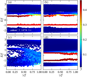
Figure 5: Eigenmodes of a finite zigzag structure, averaged over 30 random realizations of loss, as a function of loss strength $\gamma/f$ for $v/f=1$. Panels (a), (b), and (c) are computed for $t/f=-0.7$, with the numbers of sites $N=40$, $N=60$, and $N=80$, respectively. In (d), the choice of $t/f=-0.3$ facilitates resistant edge states for longer chains ($N=90$). Optimizing system parameters allows well-localized edge states even with losses’ strength as high as the system interaction. The findings stem from analyzing the finite Hamiltonian $H_{\gamma}=H+i\gamma D^{\prime}$, featuring the tight-binding Hamiltonian $H$ and the loss operator $D^{\prime}$.

Resistance to losses.—We model dissipation in the zigzag structure by a finite non-hermitian Hamiltonian $H_{\gamma}=H+i\gamma D^{\prime}$, where $\gamma$ represents losses and $D^{\prime}$ is a diagonal matrix with elements $D^{\prime}_{l,m}=\Delta d\delta_{l,m}$. We sample $\Delta d$ uniformly from $[-0.5;0.5]$.

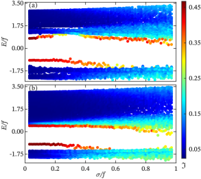
Figure 6: Our main result: robust topologically protected edge states in a zigzag system affected simultaneously by losses and disorders in next-neighbor and long-range interactions, and on-site energies; all quantified with strength $\sigma$. Remarkably, the edge states remain well localized for the disorders and losses comparable with the system interaction strength, $\sigma/f\leq 0.3$. The plot is computed for a chain of $N=60$ sites, $v/f=1$, (a) $t/f=-0.7$, (b) $t/f=-0.3$.

Fig. 5 shows eigenmodes of $H_{\gamma}$ computed for several zigzag chains, and averaged over 30 random instances of losses, as a function of the loss strength $\gamma/f$. We observe that the stability of edge states depends on $N$ along with ratios $v/f$ and $t/f$. While larger $t/f$ increases the resistance of edge states for bigger $N$, it simultaneously reduces the width of the energy gap between the edge states and bulk bands (see SM, S4). Moreover, the losses do not break the degeneracy of the edge states for a system with odd $N$. (a), (b), and (c) highlight the system’s vulnerability to losses as the number of sites increases for $t/f=-0.7$. (d) demonstrates the robustness of edge states for a chain with $t/f=-0.3$ and $N=90$. As before, $v/f=1$.

Our main result is demonstrated in Fig. 6. It shows ultra-robust topologically protected edge states obtained for the zigzag structure affected simultaneously by dissipation and all three types of disorders considered. It was obtained by an averaged simulation of the cumulative Hamiltonian $H_{\sigma}+H_{\gamma}$, where for the simplicity of computations, all the imperfections had the same strength $\sigma$. The computations were performed for $N=60$ sites with $v/f=1$, for $t/f=-0.7$ – panel (a), and $t/f=-0.3$ – panel (b). Remarkably, the edge states remain well localized for the disorders and losses comparable with the system interaction strength, $\sigma/f\leq 0.5$. Here, the negative coupling is vital for securing a distinct, resilient edge state against losses and various disorders in zigzag models of different sizes. While a certain level of resilience can be attained by relying solely on positive couplings, this comes at the cost of a smaller gap and potentially weaker localization of the edge state, allowing for simultaneous excitations in both edge and bulk states (see SM, S5). Tab. 1 compares the robustness of our edge states to the SSH, AAH, and QTI models.

Implementation.—There are several experimental platforms that can test our results. In photonic lattices [55, 56, 59, 49] , each waveguide can correspond to a site in either the A or B chains. An effective negative coupling can be induced by inserting an auxiliary defect waveguide with a precisely tuned refractive index between the two original waveguides, or by orbital-induced synthetic flux in multiorbital ($s$ and $d$ orbitals) waveguide lattices. The coupling noise can be controlled by adjusting waveguide spacing, with on-site noise modulated by varying waveguide widths, and system loss achieved by altering waveguide etch depth. Alternatively, one can use acoustic metacrystals [46], fabricating the proposed chain through 3D printing, with negative couplings formed by a special choice of unit cell connections, or superconducting circuits [67], where adjacent sites in the lattice are connected through SQUIDs and the magnetic flux can assist in manipulating the coupling sign.

	SSH	AAH	QTI	Our model
System properties
Couplings	positive	positive	positive	positive
			& negative	& negative
Topological	1-2	1-4	1-4	1-2
states	at $\varepsilon=0$	at $\varepsilon\neq 0$	at $\varepsilon=0$	at $\varepsilon\neq 0$
Self-energy	–	yes	–	yes
Robustness to disorder type
In couplings	✓	✓	✓	✓
On-site energy	–	✓	–	✓
Losses	–	–	–	✓
(dissipation)

Table 1: Robustness of topologically protected edge states obtained in the SSH, AAH, and quadrupole topological insulator (QTI) models, with these observed in the discussed zigzag structure with negative couplings. $\varepsilon$ denotes the energy level of an edge state.

Discussion and conclusions.—We demonstrated an extreme robustness of topologically protected edge states emerging from the interacting quasi-1D zigzag structure, where some of the couplings are negative. These states remain well localized in the simultaneous presence of dissipation and disorders in short- and long-range interactions, as well as in on-site energies, whose strengths are comparable with interactions in the system. We also identified several physical platforms that are capable of testing our results.

We proved non-trivial topological nature of the edge states using the bulk-boundary correspondence, despite the lack of chiral symmetry in the system. To this end, we proposed a new method that relates the original zigzag system via a continuous mapping to a ladder model featuring chiral symmetry, which is investigated in a larger, specially constructed unit cell.

The model’s simplicity and generality can make it a cornerstone for future practical quantum topology-based applications. Realization of negative couplings plays a pivotal role in broadening the range of system parameters, enabling it to support edge states, develop new symmetries, and control the energy band gap size.

Acknowledgments.—V.K. and M.S. were supported by the European Union’s Horizon 2020 research and innovation programme under the Marie Skłodowska-Curie project “AppQInfo” No. 956071. M.S. was supported by the National Science Centre “Sonata Bis” project No. 2019/34/E/ST2/00273, and the QuantERA II Programme that received funding from the European Union’s Horizon 2020 research and innovation programme under Grant Agreement No. 101017733, project “PhoMemtor” No. 2021/03/Y/ST2/00177. V.K. thanks Alexander Khanikaev for initial discussions.

SM1 Inverse participation ratio

To quantify mode localization properties, we calculate an inverse participation ratio $\mathfrak{I}$ (IPR), defined in the following way THOULESS197493_1

$$\mathfrak{I}=\left(\sum\limits_{m}\,|\psi_{m}|^{4}\right)\,\left(\sum\limits_{m}\,|\psi_{m}|^{2}\right)^{-2}.$$ (6)

Here, $\psi_{m}$ represents a mode amplitude on site $m$ in the 1D system. The mode corresponds to e.g., a field strength, voltage, pressure, or other relevant physical quantities characteristic to a physical implementation under consideration. The summation is performed over all $N$ sites within the chain.

SM2 Robustness for chains with even number of sites in the non-chiral cases

In the figures presented in the main text, we illustrate the robustness properties of a chain consisting of an even number of sites in the chiral case. Interestingly, nonchiral cases exhibit nearly the same level of robustness. However, the band gap and spectrum no longer maintain symmetry, and the influence of the bulk states on the edge states becomes noticeable at a disorder strength smaller than that in the chiral case, Fig. SM_1.

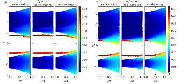
Figure SM_1: Energy eigenmodes computed for the zigzag system with $N=90$ sites, while setting $v/f=1$ and (a) $t/f=-0.7$ and (b) $t/f=-0.3$. Each case was averaged over 30 random instances of a disorder $\sigma$, for (left to right) the next-neighbour (nn) interactions, long-range (nnn) interactions, and the on-site energy.

SM3 Robustness for chains with odd number of sites in the chiral case $t/f=-1$

In the figures presented in the main text, we illustrate the robustness properties of a chain consisting of an even number of sites in the chiral case. Interestingly, the edge states can be spotted also in chains with an odd number of sites, despite its degenerate energy levels. Higher disorders in this system result in a gradual spectral spreading of edge states that remains rather insignificant, e.g., less than $1\%$ of the band gap for $\sigma/f<0.2$. It increases by $4\%$ for $\sigma/f=0.5$, and reaches $10\%$ for $\sigma/f=1$, Fig. SM_2.

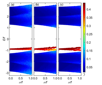
Figure SM_2: Energy eigenmodes computed for the zigzag system with $N=91$ sites, while setting $v/f=1$ and $t/f=-1$. The three panels have been averaged over 30 random instances of a disorder $\sigma$ for the (a) next-neighbour (nn) interactions, (b) long-range (nnn) interactions, and (c) the on-site energy.

SM4 Resistance to losses as optimization task

To investigate the dependence of edge state resistance to losses in the range $\gamma\in[0.0,0.1]$, we conducted calculations for $2.3\times 10^{5}$ parameter sets ${v/f,t/f,N}$, where $v/f\in[0.3,3.0]$, $t/f\in[-3.0,0.5]$, and $N\in[10,100]$. Each set underwent an initial assessment for the presence of edge states using the IPR. The results are depicted in Fig. SM_3, where the sets lacking edge states are marked in green.

Subsequently, the sets with edge states were analyzed for their ability to maintain well-localized edge states at the same energy while increasing $\gamma$ from $0$ to $0.1$. The ones exhibiting this property are labeled yellow, while those without it are marked with violet color. For clarity, all sets were grouped by their $N$ value. The black solid lines in Fig. SM_3 represent the parameter choices for the figures from the main text.

From these results, it is evident that the resistance of edge states to losses is directly correlated with $N$. The green areas in the panels of Fig. SM_3 align with the parabolic prediction from the topological invariant. Another observation is that most sets exhibit resistance within the ranges $t/f\in[-1.0,0.5]$ and $v/f\in[1.0,3.0]$. However, such strong near interactions lead to a reduction in the gap between the edge state and the closest energy band.

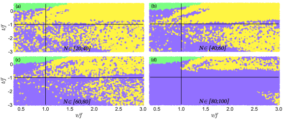
Figure SM_3: Resistance to losses for $v/f\in\left[0.3;3.0\right]$ and $t/f\in\left[-3.0;0.5\right]$. Green color represents the parameter region where the system does not support edge states, while yellow and violet regions correspond to areas with edge states, distinguishing between those that exhibit and those that do not exhibit the resistance, respectively. For simplicity, the loss resistance is defined as the property of an edge state to remain selected for the same energy within the range $\gamma\in\left[0.0;0.1\right]$. Each panel represents results based on approximately $5\times 10^{4}$ random points within the specified range of parameters $v/f$, $t/f$ and the system size (a) $N\in[20;40]$, (b) $N\in[40;60]$, (c) $N\in[60;80]$, and (d) $N\in[80;100]$. The horizontal solid line represents the chiral case $t/f=-1$, while the vertical one denotes the case of $v/f=1$.

SM5 Simultaneous presence of all types of disorder and losses in systems with positive and negative couplings

We would like to highlight that the studied system supports edge states when $t$ is both positive and negative, and these states remain robust in the presence of a certain level of disorders and losses. However, it is essential to consider the distinct nature of these edge states. Systems with different choices of $v/f$ and $t/f$ exhibit variations in localization and energy gap between the edge state and the closest bulk state. This variability is of significance for diverse implementations and applications.

In Fig. SM_4a, the system displays the largest energy gap, $\Delta\tilde{\varepsilon}=(\varepsilon_{\text{edge state}}-\varepsilon_{\text{bulk state}})/\max(\lvert v/f\rvert,\lvert t/f\rvert,1)$, with normalization aimed at ensuring the largest couplings in the Hamiltonian are less than or equal to 1. Notably, a substantial portion of the brightest region resides in the diagram’s negative $t/f$ quadrant.

Panels (b)–(d) illustrate the potential strength $\sigma$ when the system continues to support edge states at the same ($\pm 15\%$) energy level and with identical localization. Disorder and losses are introduced to the system Hamiltonian as $H_{\sigma}=H+\sigma(D+iD^{\prime})$ with operators $D$ and $D^{\prime}$, respectively. Here, the reduction in the parameter region, where the system maintains robust edge states as its size increases, is primarily associated with a decrease in resistance to losses, as predicted in Section SM4.

Figs. SM_4e–g represent the elementwise multiplication of panel (a) with panels (b)–(d), respectively. These figures distinctly indicate that the best edge states (considering localization, distance to the closest band, and robustness) are observed in systems with negative couplings. They also reveal a possibility of having edge states in zigzag chains exclusively with positive couplings, albeit with certain limitations that require attention. This paves the way to further research and simplifies the potential manufacturing process of the samples.

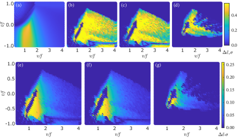
Figure SM_4: Optimization of the band gap size and robustness against simultaneous presence of all types of disorder and losses, with equal strength $\sigma$, computed for $v/f\in\left[0.3;4.1\right]$ and $t/f\in\left[-1;1\right]$. (a) Gap size $\varepsilon_{\text{edge state}}-\varepsilon_{\text{bulk state}}$ computed for the relative distance between the zigzag’s edge state and the closest band, normalized to $\max(\lvert t/f\rvert,\lvert v/f\rvert,1)$. Panels (b)–(d) depict the maximally possible strength $\sigma$ of disorder and losses, while maintaining the edge states of the zigzag model at the same ($\pm 15\%$) energy level and with an equivalent level of localization. The sizes of the systems in (b), (c), and (d) are $N=50$, $N=70$, and $N=90$, respectively. In (e)–(g), the results of element-wise multiplying the data from plot (a) by values from (b)–(d) are presented. Remarkably, the optimal choice for the most stable and remote edge states from the band edge can be achieved in models with negative couplings. However, for specific purposes, where the distance between the edge state and the band is less critical, it is possible to operate solely with positive couplings to attain a good level of resistance.

unsrt our1

References

- [1] M. Z. Hasan and C. L. Kane. Colloquium: Topological insulators. Rev. Mod. Phys., 82:3045–3067, 11 2010.
- [2] Xiao-Liang Qi and Shou-Cheng Zhang. Topological insulators and superconductors. Rev. Mod. Phys., 83:1057–1110, 10 2011.
- [3] Klaus von Klitzing, Tapash Chakraborty, Philip Kim, Vidya Madhavan, Xi Dai, James McIver, Yoshinori Tokura, Lucile Savary, Daria Smirnova, Ana Maria Rey, Claudia Felser, Johannes Gooth, and Xiaoliang Qi. 40 years of the quantum hall effect. Nat Rev Phys, 2(8):397–401, 08 2020.
- [4] Cui-Zu Chang, Chao-Xing Liu, and Allan H. MacDonald. Colloquium: Quantum anomalous hall effect. Rev. Mod. Phys., 95:011002, 01 2023.
- [5] Steven R. Elliott and Marcel Franz. Colloquium: Majorana fermions in nuclear, particle, and solid-state physics. Rev. Mod. Phys., 87:137–163, 02 2015.
- [6] M. Zahid Hasan, Guoqing Chang, Ilya Belopolski, Guang Bian, Su-Yang Xu, and Jia-Xin Yin. Weyl, dirac and high-fold chiral fermions in topological quantum matter. Nat Rev Mater, 6(9):784–803, 09 2021.
- [7] Dennis M. Nenno, Christina A. C. Garcia, Johannes Gooth, Claudia Felser, and Prineha Narang. Axion physics in condensed-matter systems. Nat Rev Phys, 2(12):682–696, 12 2020.
- [8] A.Yu. Kitaev. Fault-tolerant quantum computation by anyons. Annals of Physics, 303(1):2–30, 2003.
- [9] Chetan Nayak, Steven H. Simon, Ady Stern, Michael Freedman, and Sankar Das Sarma. Non-abelian anyons and topological quantum computation. Rev. Mod. Phys., 80:1083–1159, 09 2008.
- [10] Jiannis K. Pachos. Introduction to Topological Quantum Computation. Cambridge University Press, 2012.
- [11] Péter Boross, János K. Asbóth, Gábor Széchenyi, László Oroszlány, and András Pályi. Poor man’s topological quantum gate based on the su-schrieffer-heeger model. Phys. Rev. B, 100:045414, 07 2019.
- [12] Ville Lahtinen and Jiannis K. Pachos. A Short Introduction to Topological Quantum Computation. SciPost Phys., 3:021, 2017.
- [13] Sunil Mittal, Venkata Vikram Orre, and Mohammad Hafezi. Topologically robust transport of entangled photons in a 2d photonic system. Opt. Express, 24(14):15631–15641, 07 2016.
- [14] Mikael C. Rechtsman, Yaakov Lumer, Yonatan Plotnik, Armando Perez-Leija, Alexander Szameit, and Mordechai Segev. Topological protection of photonic path entanglement. Optica, 3(9):925–930, 09 2016.
- [15] Samuel Boutin, Pedro L. S. Lopes, Anqi Mu, Udson C. Mendes, and Ion Garate. Topological Josephson bifurcation amplifier: Semiclassical theory. J. Appl. Phys., 129(21):214302, 06 2021.
- [16] Jason Alicea, Yuval Oreg, Gil Refael, Felix von Oppen, and Matthew P. A. Fisher. Non-abelian statistics and topological quantum information processing in 1d wire networks. Nat. Phys., 7(5):412–417, 05 2011.
- [17] Andrea Blanco-Redondo, Bryn Bell, Dikla Oren, Benjamin J. Eggleton, and Mordechai Segev. Topological protection of biphoton states. Science, 362(6414):568–571, 2018.
- [18] Fulvio Flamini, Nicolo Spagnolo, and Fabio Sciarrino. Photonic quantum information processing: a review. Rep. Prog. Phys., 82(1):016001, 2018.
- [19] Jean-Luc Tambasco, Giacomo Corrielli, Robert J. Chapman, Andrea Crespi, Oded Zilberberg, Roberto Osellame, and Alberto Peruzzo. Quantum interference of topological states of light. Sci. Adv., 4(9):eaat3187, 2018.
- [20] Zengji Yue, Xiaolin Wang, and Min Gu. Topological insulator materials for advanced optoelectronic devices. Advanced Topological Insulators, pages 45–70, 2019.
- [21] Haoran Xue, Yihao Yang, and Baile Zhang. Topological valley photonics: Physics and device applications. Adv. Photonics Res., 2(8):2100013, 2021.
- [22] Hannah Price, Yidong Chong, Alexander Khanikaev, Henning Schomerus, Lukas J Maczewsky, Mark Kremer, Matthias Heinrich, Alexander Szameit, Oded Zilberberg, Yihao Yang, Baile Zhang, Andrea Alù, Ronny Thomale, Iacopo Carusotto, Philippe St-Jean, Alberto Amo, Avik Dutt, Luqi Yuan, Shanhui Fan, Xuefan Yin, Chao Peng, Tomoki Ozawa, and Andrea Blanco-Redondo. A. roadmap on topological photonics. Journal Of Physics: Photonics, 4, Jun 2022.
- [23] Viktor M. Puchnin, Olga V. Matvievskaya, Alexey P. Slobozhanyuk, Alena V. Shchelokova, and Nikita A. Olekhno. Application of topological edge states in magnetic resonance imaging. Phys. Rev. Appl., 20:024076, 08 2023.
- [24] W. P. Su, J. R. Schrieffer, and A. J. Heeger. Solitons in polyacetylene. Phys. Rev. Lett., 42:1698–1701, 06 1979.
- [25] Hajime Takayama, Y. R. Lin-Liu, and Kazumi Maki. Continuum model for solitons in polyacetylene. Phys. Rev. B, 21:2388–2393, 03 1980.
- [26] Shinsei Ryu and Yasuhiro Hatsugai. Topological origin of zero-energy edge states in particle-hole symmetric systems. Phys. Rev. Lett., 89:077002, 07 2002.
- [27] Linhu Li, Zhihao Xu, and Shu Chen. Topological phases of generalized su-schrieffer-heeger models. Phys. Rev. B, 89:085111, 02 2014.
- [28] Maria Maffei, Alexandre Dauphin, Filippo Cardano, Maciej Lewenstein, and Pietro Massignan. Topological characterization of chiral models through their long time dynamics. New J. Phys., 20(1):013023, 01 2018.
- [29] Jung-Wan Ryu, Sungjong Woo, Nojoon Myoung, and Hee Chul Park. Topological edge states in bowtie ladders with different cutting edges. Physica E: Low-dimensional Systems and Nanostructures, 137:114941, 2022.
- [30] Chen-Shen Lee, Iao-Fai Io, and Hsien chung Kao. Winding number and zak phase in multi-band ssh models. Chinese Journal of Physics, 78:96–110, 2022.
- [31] Beatriz Pérez-González, Miguel Bello, Álvaro Gómez-León, and Gloria Platero. Interplay between long-range hopping and disorder in topological systems. Phys. Rev. B, 99:035146, 01 2019.
- [32] Mor Verbin, Oded Zilberberg, Yaacov E. Kraus, Yoav Lahini, and Yaron Silberberg. Observation of topological phase transitions in photonic quasicrystals. Phys. Rev. Lett., 110:076403, 02 2013.
- [33] Yaacov E Kraus and Oded Zilberberg. Quasiperiodicity and topology transcend dimensions. Nat. Phys., 12(7):624–626, 2016.
- [34] Oded Zilberberg. Topology in quasicrystals. Opt. Mater. Express, 11(4):1143–1157, 04 2021.
- [35] Serge Aubry and Gilles André. Analyticity breaking and anderson localization in incommensurate lattices. Ann. Israel Phys. Soc, 3(133):18, 1980.
- [36] Yaacov E. Kraus, Yoav Lahini, Zohar Ringel, Mor Verbin, and Oded Zilberberg. Topological states and adiabatic pumping in quasicrystals. Phys. Rev. Lett., 109:106402, 09 2012.
- [37] Jian Li, Rui-Lin Chu, J. K. Jain, and Shun-Qing Shen. Topological anderson insulator. Phys. Rev. Lett., 102:136806, 04 2009.
- [38] Simon Stützer, Yonatan Plotnik, Yaakov Lumer, Paraj Titum, Netanel H Lindner, Mordechai Segev, Mikael C Rechtsman, and Alexander Szameit. Photonic topological anderson insulators. Nature, 560(7719):461–465, 2018.
- [39] Dmitry V. Zhirihin and Yuri S. Kivshar. Topological photonics on a small scale. Small Sci., 1(12):2100065, 2021.
- [40] Mordechai Segev and Miguel A. Bandres. Topological photonics: Where do we go from here? Nanophotonics, 10(1):425–434, 2021.
- [41] Rajesh Chaunsali, Haitao Xu, Jinkyu Yang, Panayotis G. Kevrekidis, and Georgios Theocharis. Stability of topological edge states under strong nonlinear effects. Phys. Rev. B, 103:024106, 01 2021.
- [42] Xiaotian Shi, Ioannis Kiorpelidis, Rajesh Chaunsali, Vassos Achilleos, Georgios Theocharis, and Jinkyu Yang. Disorder-induced topological phase transition in a one-dimensional mechanical system. Phys. Rev. Res., 3:033012, 07 2021.
- [43] Wladimir A. Benalcazar, B. Andrei Bernevig, and Taylor L. Hughes. Quantized electric multipole insulators. Science, 357(6346):61–66, 2017.
- [44] Nianzu Fu, Ziwei Fu, Huaiyuan Zhang, Qing Liao, Dong Zhao, and Shaolin Ke. Topological bound modes in optical waveguide arrays with alternating positive and negative couplings. Opt Quant Electron, 52(2):61, 01 2020.
- [45] Mark Kremer, Ioannis Petrides, Eric Meyer, Matthias Heinrich, Oded Zilberberg, and Alexander Szameit. A square-root topological insulator with non-quantized indices realized with photonic aharonov-bohm cages. Nat Commun, 11(1):907, 02 2020.
- [46] Xiang Ni, Mengyao Li, Matthew Weiner, Andrea Alù, and Alexander B. Khanikaev. Demonstration of a quantized acoustic octupole topological insulator. Nat Commun, 11(1):2108, 04 2020.
- [47] Danwei Liao, Zhiwang Zhang, Ying Cheng, and Xiaojun Liu. Engineering negative coupling and corner modes in a three-dimensional acoustic topological network. Phys. Rev. B, 105:184108, 05 2022.
- [48] Valerii I. Kachin and Maxim A. Gorlach. Three-dimensional higher-order topological insulator protected by cubic symmetry. Phys. Rev. Appl., 16:024032, 08 2021.
- [49] Chuang Jiang, Yiling Song, Xiaohong Li, Peixiang Lu, and Shaolin Ke. Photonic möbius topological insulator from projective symmetry in multiorbital waveguides. Opt. Lett., 48(9):2337–2340, 05 2023.
- [50] Christopher W. Peterson, Wladimir A. Benalcazar, Taylor L. Hughes, and Gaurav Bahl. A quantized microwave quadrupole insulator with topologically protected corner states. Nature, 555(7696):346–350, 03 2018.
- [51] Jean Dalibard, Fabrice Gerbier, Gediminas Juzeliūnas, and Patrik Öhberg. Colloquium: Artificial gauge potentials for neutral atoms. Rev. Mod. Phys., 83:1523–1543, 11 2011.
- [52] Xiaopeng Li, Erhai Zhao, and W. Vincent Liu. Topological states in a ladder-like optical lattice containing ultracold atoms in higher orbital bands. Nat Commun, 4(1):1523, 02 2013.
- [53] Matthieu Bellec, Ulrich Kuhl, Gilles Montambaux, and Fabrice Mortessagne. Topological transition of dirac points in a microwave experiment. Phys. Rev. Lett., 110:033902, 01 2013.
- [54] Sung Hyun Nam, Antoinette J. Taylor, and Anatoly Efimov. Diabolical point and conical-like diffraction in periodic plasmonic nanostructures. Opt. Express, 18(10):10120–10126, 05 2010.
- [55] J. M. Zeuner, M. C. Rechtsman, R. Keil, F. Dreisow, A. Tünnermann, S. Nolte, and A. Szameit. Negative coupling between defects in waveguide arrays. Opt. Lett., 37(4):533–535, 02 2012.
- [56] Robert Keil, Charles Poli, Matthias Heinrich, Jake Arkinstall, Gregor Weihs, Henning Schomerus, and Alexander Szameit. Universal sign control of coupling in tight-binding lattices. Phys. Rev. Lett., 116:213901, 05 2016.
- [57] Simon R. Pocock, Xiaofei Xiao, Paloma A. Huidobro, and Vincenzo Giannini. Topological plasmonic chain with retardation and radiative effects. ACS Photonics, 5(6):2271–2279, 06 2018.
- [58] G. Cáceres-Aravena, L. E. F. Foa Torres, and R. A. Vicencio. Topological and flat-band states induced by hybridized linear interactions in one-dimensional photonic lattices. Phys. Rev. A, 102:023505, 08 2020.
- [59] Julian Schulz, Jiho Noh, Wladimir A. Benalcazar, Gaurav Bahl, and Georg von Freymann. Photonic quadrupole topological insulator using orbital-induced synthetic flux. Nat Commun, 13(1):6597, 11 2022.
- [60] Yajuan Qi, Chunyin Qiu, Meng Xiao, Hailong He, Manzhu Ke, and Zhengyou Liu. Acoustic realization of quadrupole topological insulators. Phys. Rev. Lett., 124:206601, 05 2020.
- [61] Avik Dutt, Momchil Minkov, Ian A. D. Williamson, and Shanhui Fan. Higher-order topological insulators in synthetic dimensions. Light Sci Appl, 9(1):131, 07 2020.
- [62] Xiang Ni and Andrea Alù. Higher-order topolectrical semimetal realized via synthetic gauge fields. APL Photonics, 6(5):050802, 05 2021.
- [63] Jiacheng Bao, Deyuan Zou, Weixuan Zhang, Wenjing He, Houjun Sun, and Xiangdong Zhang. Topoelectrical circuit octupole insulator with topologically protected corner states. Phys. Rev. B, 100(20):201406(R), 11 2019.
- [64] Shuo Liu, Shaojie Ma, Qian Zhang, Lei Zhang, Cheng Yang, Oubo You, Wenlong Gao, Yuanjiang Xiang, Tie Jun Cui, and Shuang Zhang. Octupole corner state in a three-dimensional topological circuit. Light Sci Appl, 9:145, 2020.
- [65] D.J. Thouless. Electrons in disordered systems and the theory of localization. Physics Reports, 13(3):93–142, 1974.
- [66] Shinsei Ryu, Andreas P Schnyder, Akira Furusaki, and Andreas WW Ludwig. Topological insulators and superconductors: tenfold way and dimensional hierarchy. New J. Phys., 12(6):065010, 2010.
- [67] Xiu-Hao Deng, Chen-Yen Lai, and Chih-Chun Chien. Superconducting circuit simulator of bose-hubbard model with a flat band. Phys. Rev. B, 93:054116, 02 2016.
Supplemental Material: Ultra-robust topologically protected edge states in quasi-1D systems