Adaptive Mixed FEM for the Stokes eigenvalue problem

Abstract

In this paper we discuss the optimal convergence of a standard adaptive scheme based on mixed finite element approximation to the solution of the eigenvalue problem associated with the Stokes equations. The proofs of the quasi-orthogonality and the discrete reliability are presented. Our numerical experiments confirm the efficacy of the proposed adaptive scheme.

65N30, 65N25, 65N50, 76D07.

1 Introduction

Over the last few decades, the mathematical understanding of adaptive finite element methods (AFEM) has reached its maturity and adaptive schemes are more and more popular for the approximation of the solutions to partial differential equations (PDEs). Their success is based on the possibility of computing the approximated solutions of PDEs accurately with minimum number of degree of freedoms (DOFs). A rich literature confirms the huge impact of these methods in real life applications. We recall the milestone works [1, 29] for the development and analysis of a posteriori estimators which are key ingredients of adaptive algorithms.

In fluid mechanics, eigenvalue problems play a crucial role in understanding the behavior of fluid flows and their stability. Analyzing the eigenvalues provides valuable insights into the critical conditions for stability or instability in fluid flows, aiding in the design and prediction of fluid systems in various engineering applications. In this context, the numerical study of the Stokes eigenvalue problem is of great importance. Adaptive methods are designed in order to dynamically adjusts the computational resources, based on the evolving solution characteristics. Unlike static methods, adaptive techniques refine their discretization and mesh adaptively during the computation, focusing computational efforts in regions where the solution exhibits significant variations. This adaptability allows for a more efficient and accurate determination of the solutions, particularly when dealing with complex geometries or varying physical parameters. By intelligently allocating computational resources, adaptive methods enhance both the precision and the computational efficiency.

The a priori analysis of the Stokes problem is a classical topic within the theory of mixed finite elements [9]. On the other hand, the study of AFEM for the Stokes problem has been an open problem since the recent work presented in [17].

In the literature, few results based on a posteriori error estimate for the Stokes eigenvalue problem are available. In [25], it is considered a residual based a posteriori error estimator for the Stokes eigenvalue problem using stable approximations. In [24], it is presented a recovery type a posteriori error estimator for the Stokes eigenvalue problems based on projection method using some superconvergence results. Also [22, 23] deal with residual type a posteriori error estimators. In [20], a priori and a posteriori error estimates are studied, for the stress velocity formulation of the Stokes eigenvalue problem using Arnold–Winther mixed finite elements. A posteriori error estimates for divergence-conforming discontinuous Galerkin finite elements of the Stokes eigenvalue problem is discussed in [21].

The results of the present paper extend to eigenvalue problems the seminal contribution of Feischl who recently proved the optimality of a standard adaptive finite element method for the Stokes problem in [17]. One of the main contributions of [17] is the proof of the quasi-orthogonality property. Specifically, it is established a relation between the quasi-orthogonality property and the $LU$-factorization of infinite matrices. Some optimality results for adaptive mesh refinement algorithms for non-symmetric, indefinite, and time-dependent problems are discussed in [18]. More specifically, Feischl overcame one technicality in the proof of the quasi-orthogonality of [17] and presented the proof of optimality.

As far as the authors are aware, there is currently no optimality result available in the existing literature for a standard adaptive finite element method applied to the Stokes eigenvalue problems. In this paper, we introduce a suitable estimator for the Stokes eigenvalue problem which is locally equivalent to the a posteriori error estimator proposed in [25] and we prove the optimality of the standard adaptive finite element method stemming from this estimator. Specifically, we establish the four key properties discussed in [13] to ensure the rate optimality of adaptive finite element methods. In particular, we prove the quasi-orthogonality property for the numerical approximation of Stokes eigenvalue problem using the $LU$-factorization of matrices discussed in [18].

The rest of the paper is organised as follows: Section 2 is devoted to the function spaces and problem formulation. Error estimator and adaptive method will be presented in Section 3. Proof of convergence and rate optimality are discussed in Section 4. Finally, computational results are demonstrated in the Section 5.

2 The Stokes Eigenvalue problem

Let $\Omega$ be an open, bounded, and connected domain with Lipschitz boundary $\partial\Omega$. For simplicity, we assume that $\Omega$ is a polygon in two dimensions or a polyhedron in three dimensions. Let $H^{s}(\Omega)$ be the standard Sobolev space for $s\geq 0$. We denote the scalar product in $L^{2}(\Omega)=H^{0}(\Omega)$ as $(\cdot,\cdot)$. If $\omega$ is a subset of $\Omega$ then $(\cdot,\cdot)_{\omega}$ is the restriction of the scalar product to $\omega$. The following function spaces will be used to write our weak formulation:

$$\mathbf{V} =\mathbf{H}^{1}_{0}(\Omega)=\{\boldsymbol{u}\in\mathbf{H}^{1}(\Omega):\boldsymbol{u}|_{\partial\Omega}=\textbf{0}\}$$

$$Q =L^{2}_{0}(\Omega)=\left\{p\in L^{2}(\Omega):\int_{\Omega}p=0\right\}.$$

We consider the velocity-pressure Stokes eigenvalue problem: Find an eigenpair $(\boldsymbol{u},p,\lambda)$ with $\boldsymbol{u}\neq\textbf{0}$ such that

(2.1a) $$-\Delta\boldsymbol{u}+\nabla p =\lambda\boldsymbol{u}\quad\;\mbox{in}\;\Omega$$

(2.1b) $$\operatorname*{div}\boldsymbol{u} =0\qquad\mbox{in}\;\Omega$$

(2.1c) $$\boldsymbol{u} =0\qquad\mbox{on}\;\partial\Omega.$$

The standard weak formulation of the Stokes eigenvalue problem (2.1) is obtained as follows: Find $(\boldsymbol{u},p,\lambda)\in\mathbf{V}\times Q\times\mathbb{R}^{+}$ with $||\boldsymbol{u}||_{0}=1$ such that

(2.2) $$a(\boldsymbol{u},\boldsymbol{v})+b(\boldsymbol{v},p)=\lambda(\boldsymbol{u},\boldsymbol{v}) \forall\boldsymbol{v}\in\mathbf{V}$$

$$b(\boldsymbol{u},q)=0 \forall q\in Q,$$

where $a(\boldsymbol{u},\boldsymbol{v})=(\nabla\boldsymbol{u},\nabla\boldsymbol{v})$ and $b(\boldsymbol{v},p)=-(\rm{div}\,\boldsymbol{v},p)$. Throughout the paper, we will use the following graph norm:

$$|||(\boldsymbol{u},p)|||^{2}:=||\nabla\boldsymbol{u}||_{0}^{2}+||p||_{0}^{2}.$$

2.1 Discrete formulation of the Stokes eigenvalue problem

Let $\mathcal{T}$ be a shape-regular triangulation of $\Omega$. We denote by $T\in\mathcal{T}$ one element of the triangulation, by $h_{T}$ its diameter and by $h_{\mathcal{T}}$ the meshsize of $\mathcal{T}$ (maximum element diameter). We will also need the set $\mathcal{E}$ of all edges of $\mathcal{T}$ and their length $h_{e}$. When no confusion arises, $h$ will be used in place of $h_{\mathcal{T}}$.

We use the standard generalized Taylor–Hood finite element scheme [9] that is defined as $\mathbf{V}_{\mathcal{T}}^{p}\times Q_{\mathcal{T}}^{p-1}$ with $p\geq 2$, where

$$P^{p}(\mathcal{T}) :=\{v\in H^{1}(\Omega):v|_{T}\mbox{ is a polynomial with degree}\leq p,\ T\in\mathcal{T}\}$$

$$\mathbf{V}_{\mathcal{T}}^{p} :=(P^{p}(\mathcal{T}))^{2}\cap(H^{1}_{0}(\Omega))^{2},$$

$$Q_{\mathcal{T}}^{p-1} :=P^{p-1}(\mathcal{T})\cap L^{2}_{0}(\Omega).$$

The discrete weak formulation of the Stokes eigenvalue problem is defined as follows: Find $(\boldsymbol{u}_{\mathcal{T}},p_{\mathcal{T}},\lambda_{\mathcal{T}})\in\mathbf{V}_{\mathcal{T}}^{p}\times Q_{\mathcal{T}}^{p-1}\times\mathbb{R}^{+}$ with $||\boldsymbol{u}_{\mathcal{T}}||_{0}=1$ such that

(2.3) $$a(\boldsymbol{u}_{\mathcal{T}},\boldsymbol{v})+b(\boldsymbol{v},p_{\mathcal{T}})=\lambda_{\mathcal{T}}(\boldsymbol{u}_{\mathcal{T}},\boldsymbol{v}) \forall\boldsymbol{v}\in\mathbf{V}_{\mathcal{T}}^{p}$$

$$b(\boldsymbol{u}_{\mathcal{T}},q)=0 \forall q\in Q_{\mathcal{T}}^{p-1}.$$

Remark 2.1.

It the abstract theory of eigenvalue problems in mixed form, the problem is usually written in terms of an eigenspace corresponding only to the velocity space, see [10, 9]. This is convenient in order to analyze schemes that do not satisfy the inf-sup condition, thus allowing for a non-uniqueness of the pressure space. In our case, we are choosing an inf-sup stable scheme so that we decided to use a formulation of the problem where the eigenspace is associated with both the velocity and the pressure.

It is well-known that the Taylor–Hood element is inf-sup stable [9] and that its generalization to higher degrees is stable as well [6, 7, 9] In the sequel, we make the notation shorter by introducing the space

$$\mathcal{X}_{\mathcal{T}}^{p}=\mathbf{V}_{\mathcal{T}}^{p}\times Q_{\mathcal{T}}^{p-1}$$

and the corresponding notation $u_{\mathcal{T}}=(\boldsymbol{u}_{\mathcal{T}},p_{\mathcal{T}})\in\mathcal{X}_{\mathcal{T}}^{p}$ together with

$$|||u_{\mathcal{T}}|||=|||(\boldsymbol{u}_{\mathcal{T}},p_{\mathcal{T}})|||.$$

Given two subspaces $A$ and $B$ of the space $\mathcal{X}_{\mathcal{T}}^{p}$ we shall use the gap defined as

$$\delta(A,B)=\sup_{u\in A}\inf_{v\in B}|||u-v|||.$$

The stability of the numerical scheme implies then the following result.

Lemma 2.1.

For any $u_{\mathcal{T}}\in\mathcal{X}_{\mathcal{T}}^{p}$ there exits $v_{\mathcal{T}}\in\mathcal{X}^{p}_{\mathcal{T}}$ with $|||v_{\mathcal{T}}|||\leq C_{1}|||u_{\mathcal{T}}|||$ such that

(2.4) $$C_{2}|||u_{\mathcal{T}}|||\leq B(u_{\mathcal{T}},v_{\mathcal{T}})$$

where $B(u_{\mathcal{T}},v_{\mathcal{T}})=a(\boldsymbol{u}_{\mathcal{T}},\boldsymbol{v}_{\mathcal{T}})-b(\boldsymbol{v}_{\mathcal{T}},p_{\mathcal{T}})-b(\boldsymbol{u}_{\mathcal{T}},q_{\mathcal{T}})$ and, $C_{1}$ and $C_{2}$ are positive constants independent of $h_{\mathcal{T}}$.

Proof.

Employing the inf-sup condition in conjunction with the definition of the bilinear form $B(\cdot,\cdot)$ yields the stated outcome.

Lemma 2.2.

There holds:

(2.5) $$B(u_{\mathcal{T}},v_{\mathcal{T}})\leq C_{b}|||u_{\mathcal{T}}|||\,|||v_{\mathcal{T}}|||\quad\forall u_{\mathcal{T}},v_{\mathcal{T}}\in\mathcal{X}_{\mathcal{T}}^{p}.$$

Proof.

An application of Cauchy-Schwarz implies the stated result.

Lemma 2.3.

There holds:

(2.6) $$||\boldsymbol{u}-\boldsymbol{u}_{\mathcal{T}}||_{0}\leq\rho(h_{\mathcal{T}})|||u-u_{\mathcal{T}}|||,$$

where $\rho(h_{\mathcal{T}})$ tends to zero as $h_{\mathcal{T}}$ tends to zero.

Proof.

Applying the $L^{2}$ error estimate derived in [28] in conjunction with eigenvalue findings from [3] and [8] results in the presented conclusion.

Theorem 2.1 (Identity I).

Let $(\boldsymbol{u},p,\lambda)\in\mathbf{V}\times Q\times\mathbb{R}^{+}$ and $(\boldsymbol{u}_{\mathcal{T}},p_{\mathcal{T}},\lambda_{\mathcal{T}})\in\mathbf{V}_{\mathcal{T}}\times Q_{\mathcal{T}}\times\mathbb{R}^{+}$ be solutions of the weak formulations (2.2) and (2.3), respectively. Then the following identity holds:

$$\lambda_{\mathcal{T}}-\lambda$$

$$\quad=a(\boldsymbol{u}-\boldsymbol{u}_{\mathcal{T}},\boldsymbol{u}-\boldsymbol{u}_{\mathcal{T}})-b(\boldsymbol{u}-\boldsymbol{u}_{\mathcal{T}},p-p_{\mathcal{T}})-b(\boldsymbol{u}-\boldsymbol{u}_{\mathcal{T}},p-p_{\mathcal{T}})-\lambda||\boldsymbol{u}-\boldsymbol{u}_{\mathcal{T}}||_{0}^{2}.$$

Proof.

Note that

$$a(\boldsymbol{u}-\boldsymbol{u}_{\mathcal{T}},\boldsymbol{u}-\boldsymbol{u}_{\mathcal{T}})-b(\boldsymbol{u}-\boldsymbol{u}_{\mathcal{T}},p-p_{\mathcal{T}})-b(\boldsymbol{u}-\boldsymbol{u}_{\mathcal{T}},p-p_{\mathcal{T}})$$

$$\quad=a(\boldsymbol{u},\boldsymbol{u})-b(\boldsymbol{u},p)-b(\boldsymbol{u},p)+a(\boldsymbol{u}_{\mathcal{T}},\boldsymbol{u}_{\mathcal{T}})-b(\boldsymbol{u}_{\mathcal{T}},p_{\mathcal{T}})-b(\boldsymbol{u}_{\mathcal{T}},p_{\mathcal{T}})$$

$$\qquad-2(a(\boldsymbol{u},\boldsymbol{u}_{\mathcal{T}})-b(\boldsymbol{u},p_{\mathcal{T}})-b(\boldsymbol{u}_{\mathcal{T}},p))$$

$$\quad=\lambda(\boldsymbol{u},\boldsymbol{u})+\lambda_{\mathcal{T}}(\boldsymbol{u}_{\mathcal{T}},\boldsymbol{u}_{\mathcal{T}})-2\lambda(\boldsymbol{u},\boldsymbol{u}_{\mathcal{T}}).$$

Using

$$\lambda(\boldsymbol{u}-\boldsymbol{u}_{\mathcal{T}},\boldsymbol{u}-\boldsymbol{u}_{\mathcal{T}})=\lambda(\boldsymbol{u},\boldsymbol{u})+\lambda(\boldsymbol{u}_{\mathcal{T}},\boldsymbol{u}_{\mathcal{T}})-2\lambda(\boldsymbol{u},\boldsymbol{u}_{\mathcal{T}})$$

gives

$$a(\boldsymbol{u}-\boldsymbol{u}_{\mathcal{T}},\boldsymbol{u}-\boldsymbol{u}_{\mathcal{T}})-b(\boldsymbol{u}-\boldsymbol{u}_{\mathcal{T}},p-p_{\mathcal{T}})-b(\boldsymbol{u}-\boldsymbol{u}_{\mathcal{T}},p-p_{\mathcal{T}})$$

$$\quad=-\lambda(\boldsymbol{u}_{\mathcal{T}},\boldsymbol{u}_{\mathcal{T}})+\lambda_{\mathcal{T}}(\boldsymbol{u}_{\mathcal{T}},\boldsymbol{u}_{\mathcal{T}})+\lambda(\boldsymbol{u}-\boldsymbol{u}_{\mathcal{T}},\boldsymbol{u}-\boldsymbol{u}_{\mathcal{T}}).$$

This completes the proof.

Similarly, we can prove the following identity.

Theorem 2.2 (Identity II).

Let $\widehat{\mathcal{T}}\in\mathbb{T}$ be any refinement of a given triangulation $\mathcal{T}\in\mathbb{T}$. Let $(\boldsymbol{u}_{\widehat{\mathcal{T}}},p_{\widehat{\mathcal{T}}},\lambda_{\widehat{\mathcal{T}}})\in\mathbf{V}_{\widehat{\mathcal{T}}}\times Q_{\widehat{\mathcal{T}}}\times\mathbb{R}^{+}$ and $(\boldsymbol{u}_{\mathcal{T}},p_{\mathcal{T}},\lambda_{\mathcal{T}})\in\mathbf{V}_{\mathcal{T}}\times Q_{\mathcal{T}}\times\mathbb{R}^{+}$ be solutions of the discrete weak formulation (2.3). Then the following identity holds:

$$\lambda_{\mathcal{T}}-\lambda_{\widehat{\mathcal{T}}} =a(\boldsymbol{u}_{\widehat{\mathcal{T}}}-\boldsymbol{u}_{\mathcal{T}},\boldsymbol{u}_{\widehat{\mathcal{T}}}-\boldsymbol{u}_{\mathcal{T}})-b(\boldsymbol{u}_{\widehat{\mathcal{T}}}-\boldsymbol{u}_{\mathcal{T}},p_{\widehat{\mathcal{T}}}-p_{\mathcal{T}})-b(\boldsymbol{u}_{\widehat{\mathcal{T}}}-\boldsymbol{u}_{\mathcal{T}},p_{\widehat{\mathcal{T}}}-p_{\mathcal{T}})$$

$$\quad-\lambda_{\widehat{\mathcal{T}}}||\boldsymbol{u}_{\widehat{\mathcal{T}}}-\boldsymbol{u}_{\mathcal{T}}||_{0}^{2}.$$

3 Error estimator and adaptive scheme

In this section we introduce the a posteriori error estimator that we are using in our adaptive scheme and we state our main convergence and optimality theorem. We are also recalling the main tools needed for the proof in the spirit of [16, 15, 11]. The actual proof of all the auxiliary results is postponed to the next section for the sake of readability.

In [19, 17, 18], a residual based a posteriori error estimator for the Stokes source problem, is discussed. That estimator is locally equivalent to the a posteriori error estimator proposed by Verfürth in [29]. The locally equivalency between the two estimators follows directly from the following estimates:

(3.1) $$||\operatorname*{div}\boldsymbol{u}||^{2}_{L^{2}(\Omega)}\leq C_{11}\sum_{e\in\mathcal{E}}h_{e}||[\partial_{n}\boldsymbol{u}_{\mathcal{T}}]||^{2}_{L^{2}(e)}$$

and

(3.2) $$||\operatorname*{div}\boldsymbol{u}_{\mathcal{T}}|_{T}||^{2}_{L^{2}(\partial T)}\leq C_{12}h_{T}^{-1/2}||\operatorname*{div}\boldsymbol{u}||^{2}_{L^{2}(T)},$$

where $C_{11}$ and $C_{12}$ are positive constants. For more details, see also [19, 27, 4].

We introduce a new estimator for the Stokes eigenvalue problem which is locally equivalent to one proposed in [25]. Specifically, our adaptive scheme is based on the following local error estimator for all $T\in\mathcal{T}$:

(3.3) $$\eta_{T}^{2} :=h_{T}^{2}||\lambda_{\mathcal{T}}\boldsymbol{u}_{\mathcal{T}}+\Delta\boldsymbol{u}_{\mathcal{T}}-\nabla p_{\mathcal{T}}||_{L^{2}(T)}^{2}$$

$$\quad+h_{T}||[\partial_{n}\boldsymbol{u}_{\mathcal{T}}]||^{2}_{L^{2}(\partial{T}\cap\Omega)}+h_{T}||\operatorname*{div}\boldsymbol{u}_{\mathcal{T}}|_{T}||^{2}_{L^{2}(\partial T)}.$$

Given a triangulation $\mathcal{T}$, our global estimator reads as

(3.4) $$\eta(\mathcal{T}):=\left(\sum_{T\in\mathcal{T}}\eta_{T}^{2}\right)^{1/2}.$$

For a set of elements $\mathcal{M}$, we define the notation $\eta(\mathcal{M})$ as

(3.5) $$\eta(\mathcal{M}):=\left(\sum_{T\in\mathcal{M}}\eta_{T}^{2}\right)^{1/2}.$$

In order to keep our notation lighter, we consider a simple eigenvalue (that is, an eigenvalue with multiplicity $1$). This fact has been already used implicitly in the definition of the estimator. More general situations could be considered in the spirit of [11].

Let $\lambda$ be a simple eigenvalue with the associated one dimensional eigenspace $W={\rm\textbf{span}}(u)$ with $u=(\boldsymbol{u},p)$. Let $\lambda_{\mathcal{T}}$ be the approximated (discrete) eigenvalue with the associated one dimensional eigenspace $W_{\mathcal{T}}={\rm\textbf{span}}(u_{\mathcal{T}})$ with $u_{\mathcal{T}}=(\boldsymbol{u}_{\mathcal{T}},p_{\mathcal{T}})$. We are interested in estimating the error in the eigenvalue approximation $|\lambda-\lambda_{\mathcal{T}}$ and the gap between the continuous eigenspace $W$ and the approximated eigenspace $W_{\mathcal{T}}$ $\delta(W,W_{\mathcal{T}})$.

Next, we state the reliability and the efficiency results for our a posteriori estimator.

Proposition 3.1.

Let $(u,\lambda)=(\boldsymbol{u},p,\lambda)$ and $(u_{\mathcal{T}},\lambda_{\mathcal{T}})=(\boldsymbol{u}_{\mathcal{T}},p_{\mathcal{T}},\lambda_{\mathcal{T}})$ be the continuous solution of (2.2) and the discrete solution of (2.3), respectively. Then, the following reliability estimate holds:

(3.6) $$|||u-u_{\mathcal{T}}||| \leq C(\eta(\mathcal{T})+|\lambda-\lambda_{\mathcal{T}}|+\lambda||\boldsymbol{u}-\boldsymbol{u}_{\mathcal{T}}||_{0}),$$

(3.7) $$|\lambda-\lambda_{\mathcal{T}}| \leq C(\eta(\mathcal{T})^{2}+|\lambda-\lambda_{\mathcal{T}}|^{2}+\lambda^{2}||\boldsymbol{u}-\boldsymbol{u}_{\mathcal{T}}||_{0}^{2})$$

where $C$ is a positive constant independent of the mesh size $h_{\mathcal{T}}$. Moreover, the following local efficiency result holds:

(3.8) $$\eta_{T}\leq C\left(|||u-u_{\mathcal{T}}|||_{\omega(T)}+\sum_{T^{\prime}\subset\omega(T)}h_{T^{\prime}}^{1/2}(|\lambda-\lambda_{\mathcal{T}}|+\lambda||\boldsymbol{u}-\boldsymbol{u}_{\mathcal{T}}||_{0,T^{\prime}})\right),$$

where $\omega(T)$ is the union of all elements that share at least one edge $(d=2)$ or one face $(d=3)$ with T.

Proof.

Note that our estimator for the Stokes eigenvalue problem is locally equivalent to the a posteriori error estimator proposed in [25] with (3.1) and (3.2). Hence, the stated results directly follows from the reliability and the efficiency results discussed in [25].

Corollary 3.1.

The following reliability estimates hold:

(3.9) $$|||u-u_{\mathcal{T}})||| \leq C\eta(\mathcal{T})+\rho_{rel1}(h_{\mathcal{T}})|||u-u_{\mathcal{T}}|||,$$

(3.10) $$|\lambda-\lambda_{\mathcal{T}}| \leq C\eta(\mathcal{T})^{2}+\rho_{rel2}(h_{\mathcal{T}})|||u-u_{\mathcal{T}}|||^{2}$$

where $\rho_{rel1}(h_{)}$ and $\rho_{rel2}(h)$ tend to zero as $h$ tends to zero. Moreover, it also holds:

(3.11) $$\eta_{T}\leq C|||u-u_{\mathcal{T}}|||_{\omega(T)}.$$

Proof.

Combining Proposition 3.1 and (2.6) leads the stated result.

We consider a standard adaptive scheme based on the error estimator (3.3) and on the usual paradigm SOLVE–ESTIMATE–MARK–REFINE. We describe it Algorithm 1, where we use the short notation $\bullet_{\ell}$ for $\bullet_{\mathcal{T}_{\ell}}$. In practice, Algorithm 1 should be combined with a suitable stopping criterion associated to a given error tolerance.

Algorithm 1: Adaptive FEM for the Stokes eigenvalue problem
Input Given initial mesh $\mathcal{T}_{0}$ and parameter $0<\theta<1$.
For $\ell=0,1,\cdots$ do:

• Solve: Compute $(\boldsymbol{u}_{\ell},p_{\ell},\lambda_{\ell})$ from (2.3)

• Estimate: Compute $\eta_{T}$ for all $T\in\mathcal{T}_{\ell}$

• Mark: Obtain a set $\mathcal{M}_{\ell}\subseteq\mathcal{T}_{\ell}$ with minimum cardinality such that

  $$\eta(\mathcal{M}_{\ell})^{2}\geq\theta\eta(\mathcal{T}_{\ell})^{2}$$

• Refine: Apply newest-vertex-bisection to refine $\mathcal{T}_{\ell}$ and to obtain a new mesh $\mathcal{T}_{\ell+1}$

Output: Sequence of meshes $\mathcal{T}_{\ell}$ and corresponding approximations of the eigenvalue $\lambda_{\ell}$ and the eigenfunction $(\boldsymbol{u}_{\ell},p_{\ell})$.

We are now in a position to introduce and state the main result of our paper. The convergence of the adaptive scheme is usually assessed by considering nonlinear approximation classes, see [5]. In particular, we are going to use the following semi-norm

$$|W|_{\mathcal{A}_{s}}=\sup_{m\in\mathbb{N}}m^{s}\inf_{\begin{subarray}{c}\mathcal{T}\in\mathbb{T}\\ card(\mathcal{T})=m\end{subarray}}\delta(W,\mathcal{X}^{p}_{\mathcal{T}}),$$

where $\mathbb{T}$ is the set of admissible triangulations and the cardinality $card(\mathcal{T})$ is the number of elements of the mesh $\mathcal{T}$.

Theorem 3.1.

Let $\mathcal{T}_{\ell}$ be the sequence of meshes generated by Algorithm 1 with bulk parameter $\theta\in(0,1)$ starting from a given mesh $\mathcal{T}_{0}$. If the continuous eigenspace $W$ has bounded $\mathcal{A}_{s}$-seminorm for some $s$ ,i.e. $|W|_{\mathcal{A}_{s}}<\infty$, then the output of the adaptive scheme satisifies the following optimal estimate:

(3.12) $$\delta(W,W_{\ell})\leq C(card(\mathcal{T}_{\ell})-card(\mathcal{T}_{0}))^{-s}|W|_{\mathcal{A}}^{s}.$$

Moreover, it also holds:

(3.13) $$|\lambda-\lambda_{\ell}|\leq C\,\delta(W,W_{\ell})^{2}.$$

The proof of the theorem together with the proof of a series of preparatory results, will be given in Section 4

4 Proof of convergence and rate optimality

We follow the abstract setting used in [12], see also [13]. Hence, the result of Theorem 3.1 follows from a series of preparatory results that we are going to state and prove in this section.

Proposition 4.1 (Stability on nonrefined elements).

Let $\widehat{\mathcal{T}}\in\mathbb{T}$ be any refinement of a given triangulation $\mathcal{T}\in\mathbb{T}$ and $S\subseteq\mathcal{T}\cap\widehat{\mathcal{T}}$ be the set of the nonrefined elements. Then

(4.1) $$\left|\left(\sum_{T\in S}\eta_{T}(\widehat{\mathcal{T}})^{2}\right)^{1/2}-\left(\sum_{T\in S}\eta_{T}(\mathcal{T})^{2}\right)^{1/2}\right|\leq C_{stab}|||u_{\widehat{\mathcal{T}}}-u_{\mathcal{T}}|||.$$

Proof.

Let $\widehat{\mathcal{T}}\in\mathbb{T}$ be any refinement of the given triangulation $\mathcal{T}\in\mathbb{T}$ and $S\subseteq\mathcal{T}\cap\widehat{\mathcal{T}}$ be the set of the nonrefined elements. Then

$$\left(\sum_{T\in S}\eta_{T}(\widehat{\mathcal{T}})^{2}\right)^{1/2}\leq\left(\sum_{T\in S}\eta_{T}(\mathcal{T})^{2}\right)^{1/2}$$

$$\quad+\Bigg{(}\sum_{T\in S}\big{(}h_{T}^{2}||\lambda_{\widehat{\mathcal{T}}}\boldsymbol{u}_{\widehat{\mathcal{T}}}+\Delta\boldsymbol{u}_{\widehat{\mathcal{T}}}-\nabla p_{\widehat{\mathcal{T}}}-(\lambda_{\mathcal{T}}\boldsymbol{u}_{\mathcal{T}}+\Delta\boldsymbol{u}_{\mathcal{T}}-\nabla p_{\mathcal{T}})||_{L^{2}(T)}^{2}$$

$$\qquad\quad+h_{T}||[\partial_{n}(\boldsymbol{u}_{\widehat{\mathcal{T}}}-\boldsymbol{u}_{\mathcal{T}})]||^{2}_{L^{2}(\partial{T}\cap\Omega)}+h_{T}||\operatorname*{div}(\boldsymbol{u}_{\widehat{\mathcal{T}}}-\boldsymbol{u}_{\mathcal{T}})|_{T}||^{2}_{L^{2}(\partial T)}\big{)}\Bigg{)}^{1/2}.$$

Using the efficiency bound implies the stated results.

Proposition 4.2 (Reduction property on refined elements).

For any refinement $\widehat{\mathcal{T}}\in\mathbb{T}$ of the given triangulation $\mathcal{T}\in\mathbb{T}$, the following condition holds:

(4.2) $$\sum_{T\in\widehat{\mathcal{T}}\setminus\mathcal{T}}\eta_{T}(\widehat{\mathcal{T}})^{2}\leq q_{red}\sum_{T\in\mathcal{T}\setminus\widehat{\mathcal{T}}}\eta_{T}(\mathcal{T})^{2}+C_{red}|||u_{\widehat{\mathcal{T}}}-u_{\mathcal{T}}|||^{2}.$$

Proof.

Let $\widehat{\mathcal{T}}\in\mathbb{T}$ be any refinement of the given triangulation $\mathcal{T}\in\mathbb{T}$. For any $\delta>0$, using standard arguments from [14, 19, 12] gives

$$\sum_{T\in\widehat{\mathcal{T}}}\eta_{T}(\widehat{\mathcal{T}})^{2}\leq(1+\delta)\sum_{T\in\mathcal{T}}\eta_{T}(\mathcal{T})^{2}-\tau(1+\delta)\sum_{T\in\mathcal{T}\setminus\widehat{\mathcal{T}}}\eta_{T}(\mathcal{T})^{2}+C_{\delta}|||(u_{\widehat{\mathcal{T}}}-u_{\mathcal{T}}|||^{2},$$

where $C_{\delta}$ is a positive constant which may depend on $\delta$ and $\tau$ is a positive constant which does not depend of $\delta$. Let $\theta\in(0,1]$ be the marking parameter used in the following condition

$$\theta\sum_{T\in\mathcal{T}}\eta_{T}(\mathcal{T})^{2}\leq\sum_{T\in\mathcal{T}\setminus\widehat{\mathcal{T}}}\eta_{T}(\mathcal{T})^{2}.$$

Hence, we obtain

$$\sum_{T\in\widehat{\mathcal{T}}}\eta_{T}(\widehat{\mathcal{T}})^{2}\leq(1+\delta)(1-\tau\theta)\sum_{T\in\mathcal{T}}\eta_{T}(\mathcal{T})^{2}+C_{\delta}|||u_{\widehat{\mathcal{T}}}-u_{\mathcal{T}}|||^{2}.$$

Choosing the parameter $\delta$ small enough, there exists a $\Theta$ with $\Theta<1$ such that

$$\sum_{T\in\widehat{\mathcal{T}}}\eta_{T}(\widehat{\mathcal{T}})^{2}\leq\Theta\sum_{T\in\mathcal{T}}\eta_{T}(\mathcal{T})^{2}+C_{\delta}|||(\boldsymbol{u}_{\widehat{\mathcal{T}}}-\boldsymbol{u}_{\mathcal{T}},p_{\widehat{\mathcal{T}}}-p_{\mathcal{T}})|||^{2}.$$

Combining the estimate with the stability on non-refined elements, leads to the desired result.

Proposition 4.3 (Generalized quasi-orthogonality).

For sufficiently small $\epsilon\geq 0$, the output of Algorithm 1 satisfies for all $\ell$ and $N\in\mathbb{N}$

(4.3) $$\sum_{k=0}^{N}||u_{\ell+k+1}-u_{\ell+k}||^{2}_{\mathcal{X}}\leq C(N)||u-u_{\ell}||^{2}_{\mathcal{X}}+\rho_{2}(h_{\ell})\sum_{k=0}^{N}||u-u_{\ell+k}||^{2}_{\mathcal{X}}$$

where $\rho_{2}(h)$ tends to zero as $h$ goes to zero and $C(N)=o(N)$ as $N\rightarrow\infty$. Further details regarding $C(N)$ can be found in [18, Eq. (8)].

Proof.

The proof of this proposition is the consequence of the following definitions and lemmas.

First we introduce some notation of the block structures of matrices.

Definition 4.1.

In the context of a block structure where there are numbers $n_{1},n_{2},\ldots\in\mathbb{N}$ with $n_{1}=1$ and $n_{i}<n_{j}$ for all $i<j$, we refer to matrix blocks as follows:

$$A(i,j):=A|_{\{n_{i},\cdots,n_{i+1-1}\}\times\{n_{j},\ldots,n_{j+1}-1\}}\in\mathbb{R}^{(n_{i+1}-n_{i})\times(n_{j+1}-n_{j})}.$$

Therefore, we represent the restriction of matrix $A$ to the initial $(k+1)\times(k+1)$ blocks as $A[k]:=A(0:k,0:k)\in\mathbb{R}^{(n_{k+1})\times(n_{k+1})}$.

An infinite matrix $A\in\mathbb{R}^{\mathbb{N}\times\mathbb{N}}$ admits the $LU$-decomposition (or factorization) if A satisfies the condition $A=LU$ for $L,U\in\color[rgb]{0,0,1}\mathbb{R}^{\mathbb{N}\times\mathbb{N}}$ with

$$L_{ii}=1,\quad L_{ij}=U_{ji}=0\ \forall i,j\in\mathbb{N},\ i<j.$$

Using Definition 4.1 of a block structure, we can say that $A$ admits a block $LU$-factorization if $A=LU$ and $L$ and $U$ satisfy

$$L(i,i)=I,\quad L(i,j)=U(j,i)=0\mbox{ with }i,j\in\mathbb{N},\ i<n_{r}\leq j\mbox{ for some }r.$$

Our aim is to reformulate the original problem into matrix framework using a hierarchical basis. In order to prove the (4.3), we require the spaces $\mathcal{X}_{\ell},\mathcal{X}_{\ell+1},\cdots,\mathcal{X}_{\ell+N+1}$ for specified $\ell,N\in\mathbb{N}$.

Definition 4.2 (Nested orthogonal basis $\mathcal{B}^{\mathcal{X}}$ ).

Given two natural numbers $\ell,N\in\mathbb{N}$, and a nested sequence of spaces $\mathcal{X}_{\ell},\mathcal{X}_{\ell+1},\dots,\mathcal{X}_{\ell+N+1}$ generated by Algorithm 1, we can construct a nested orthonormal basis $\mathcal{B}^{\mathcal{X}}$ (which depends on $\ell$ and $N$) by following these steps:

• Start with an orthonormal basis $\mathcal{B}^{\mathcal{X}}_{0}$ for the initial space $\mathcal{X}_{\ell}$.

• For each subsequent space $\mathcal{X}_{\ell+j}$ (where $j=1,2,\ldots,N+1$), construct an orthonormal basis $\mathcal{B}^{\mathcal{X}}_{j}$ that:

  $$\{v\in\mathcal{X}_{\ell+j}:v\perp^{\mathcal{X}}\mathcal{X}_{\ell+j-1}\}\quad\forall j=1,\ldots,N+1.$$

• Combine the basis vectors from all $\mathcal{B}^{\mathcal{X}}_{j}$ to form the nested orthonormal basis $\mathcal{B}^{\mathcal{X}}:=\bigcup_{j=0}^{N+1}\mathcal{B}^{\mathcal{X}}_{j}$.

Next we state the sufficient condition for the existence of the block $LU$-factorization that is called the matrix inf-sup condition

$$\sup_{k\in\mathbb{N}}||(A[k])^{-1}||_{2}=C_{\text{inf-sup}}<\infty.$$

Lemma 4.3.

For given $\ell,N\in\mathbb{N}$, let $A\in\mathbb{R}^{\dim(\mathcal{X}_{\ell+N+1})\times\dim(\mathcal{X}_{\ell+N+1})}$ be a block matrix defined by

$$A_{ij}=B(w_{j}^{\mathcal{X}},w_{i}^{\mathcal{X}}),\quad\mbox{ for all }1\leq i,j\leq\dim(\mathcal{X}_{\ell+N+1})$$

If $A$ has a Block LU factorization, then the general quasi-orthogonality $(\ref{gqo})$ holds with

$$C(N)\leq\frac{C_{b}^{2}}{\gamma^{2}}||U||_{\ell_{2}}^{2}\sup_{k=1,\ldots,N+1}||U^{-1}(:,k+1)||_{\ell_{2}}^{2}\sup_{k}\left|\frac{\lambda_{\ell+k+1}}{\lambda_{\ell+N+1}}\right|,$$

where $C_{b}$ and $\gamma=C_{2}/C_{1}$ are defined in (2.5) and (2.1), respectively.

Proof 4.4.

To express the discrete problem (2.3) in matrix form over $\mathcal{T}_{\ell},\mathcal{T}_{\ell+1},\dots,\mathcal{T}_{\ell+N+1}$, we utilize Definition 4.2 in the following manner: We define $X(k)\in\mathbb{R}^{n_{k+1}}$ for $0\leq k\leq N+1$, ensuring that $u_{\ell+k}$ can be represented as $\sum_{k=0}^{n_{k+1}}X(k)_{n}w_{n}^{\mathcal{X}}$. With this, the matrix form of the weak formulation can be expressed as:

$$A[k]X(k)=\lambda_{\ell+k}M[k]X(k)\quad\mbox{for all }k=0,\ldots,N+1,$$

where

$$X(k):=(X(k)_{1},X(k)_{2},\ldots,X(k)_{n_{k}+1})$$

with $A[k]=L[k]U[k]$ for any block $LU$-factorization. Moreover, it holds for all $1\leq i\leq n_{k+1}$:

$$(L[k]U[k]X(k))_{i} =(A[k]X(k))_{i}=\lambda_{\ell+k}(M[k]X(k))_{i}=\lambda_{\ell+k}(MX(N+1))_{i}$$

$$=\frac{\lambda_{\ell+k}}{\lambda_{\ell+N+1}}(\lambda_{\ell+N+1}MX(N+1))_{i}=\frac{\lambda_{\ell+k}}{\lambda_{\ell+N+1}}(LUX(N+1))_{i}.$$

Since $L[k]$ and $L$ are regular, we have that, for $0\leq k\leq N+1$,

$$(U[k]X(k))_{i}=\frac{\lambda_{\ell+k}}{\lambda_{\ell+N+1}}(UX(N+1))_{i}\quad\mbox{for all }1\leq i\leq n_{k+1}.$$

Furthermore, it holds that $(UX(k))i=0$ for $i>n_{k+1}$. It is important to emphasize that $\mathcal{B}^{\mathcal{X}}$ exhibits $\mathcal{X}$-orthogonality. Subsequently,

$$||u_{\ell+k+1}-u_{\ell+k}||_{\mathcal{X}}^{2}=||X(k+1)-X(k)||_{\ell_{2}}^{2}=||U^{-1}(UX(k+1)-UX(k))||_{\ell_{2}}^{2}.$$

Therefore, it can be deduced:

$$||u_{\ell+k+1}-u_{\ell+k}||_{\mathcal{X}}^{2}$$

$$\quad\leq||U^{-1}(:,k+1)||_{2}\left\|\frac{\lambda_{\ell+k+1}}{\lambda_{\ell+N+1}}(UX)(k+1)-\frac{\lambda_{\ell+k}}{\lambda_{\ell+N+1}}(UX)(k)\right\|_{l_{2}}^{2}$$

$$\quad\leq||U^{-1}(:,k+1)||_{2}$$

$$\qquad\left(\left|\frac{\lambda_{\ell+k+1}}{\lambda_{\ell+N+1}}\right|^{2}||(UX)(k+1)-(UX)(k)||_{l_{2}}^{2}+\left|\frac{\lambda_{\ell+k+1}-\lambda_{\ell+k}}{\lambda_{\ell+N+1}}\right|^{2}||(UX)(k)||_{l_{2}}^{2}\right)$$

$$\quad\leq||U^{-1}(:,k+1)||_{2}$$

$$\qquad\left(\left|\frac{\lambda_{\ell+k+1}}{\lambda_{\ell+N+1}}\right|^{2}||(UX(N+1))|_{n_{k+1}+1:n_{k+2}}||_{l_{2}}^{2}+\left|\frac{\lambda_{\ell+k+1}-\lambda_{\ell+k}}{\lambda_{\ell+N+1}}\right|^{2}||(UX)(k)||_{l_{2}}^{2}\right).$$

Moreover, we can conclude that

$$\sum_{k=0}^{N}||u_{\ell+k+1}-u_{\ell+k}||_{\mathcal{X}}^{2}$$

$$\quad\leq\max_{k=0,\ldots,N}||U^{-1}(:,k+1)||_{2}$$

$$\qquad\left(\sum_{k=0}^{N}\left|\frac{\lambda_{\ell+k+1}}{\lambda_{\ell+N+1}}\right|^{2}||(UX(N+1))|_{n_{k+1}+1:n_{k+2}}||_{l_{2}}^{2}+\sum_{k=0}^{N}\left|\frac{\lambda_{\ell+k+1}-\lambda_{\ell+k}}{\lambda_{\ell+N+1}}\right|^{2}||(UX)(k)||_{l_{2}}^{2}\right)$$

$$\quad\leq\max_{k=0,\ldots,N}||U^{-1}(:,k+1)||_{2}$$

$$\qquad\left(\sup_{k}\left|\frac{\lambda_{\ell+k+1}}{\lambda_{\ell+N+1}}\right|^{2}||(UX(N+1))|_{n_{1}+1:n_{N+2}}||_{l_{2}}^{2}+\sum_{k=0}^{N}\left|\frac{\lambda_{\ell+k+1}-\lambda_{\ell+k}}{\lambda_{\ell+N+1}}\right|^{2}||(UX)(k)||_{l_{2}}^{2}\right)$$

$$\quad=\max_{k=0,\ldots,N}||U^{-1}(:,k+1)||_{2}$$

$$\qquad\left(\sup_{k}\left|\frac{\lambda_{\ell+k+1}}{\lambda_{\ell+N+1}}\right|^{2}||UX(N+1)-UX(0)||_{l_{2}}^{2}+\sum_{k=0}^{N}\left|\frac{\lambda_{\ell+k+1}-\lambda_{\ell+k}}{\lambda_{\ell+N+1}}\right|^{2}||(UX)(k)||_{l_{2}}^{2}\right)$$

$$\quad\leq||U||_{2}^{2}\max_{k=0,\ldots,N}||U^{-1}(:,k+1)||_{2}$$

$$\qquad\left(\sup_{k}\left|\frac{\lambda_{\ell+k+1}}{\lambda_{\ell+N+1}}\right|^{2}||X(N+1)-X(0)||_{l_{2}}^{2}+\sum_{k=0}^{N}\left|\frac{\lambda_{\ell+k+1}-\lambda_{\ell+k}}{\lambda_{\ell+N+1}}\right|^{2}\right)$$

A simple application of the discrete inf-sup stabilty with (2.6) gives

$$||X(N+1)-X(0)||_{l_{2}}^{2}=||u_{\ell+N+1}-u_{\ell}||_{\mathcal{X}}^{2}\leq C(||u-u_{\ell}||_{\mathcal{X}}^{2}+|\lambda-\lambda_{\ell+N+1}|),$$

which implies

$$\sum_{k=0}^{N}||u_{\ell+k+1}-u_{\ell+k}||_{\mathcal{X}}^{2}$$

$$\quad\leq||U||_{2}^{2}\max_{k=0,\ldots,N}||U^{-1}(:,k+1)||_{2}$$

$$\qquad\left(\sup_{k}\left|\frac{\lambda_{\ell+k+1}}{\lambda_{\ell+N+1}}\right|^{2}C(||u-u_{\ell}||_{\mathcal{X}}^{2}+|\lambda-\lambda_{\ell+N+1}|)+\sum_{k=0}^{N}\left|\frac{\lambda_{\ell+k+1}-\lambda_{\ell+k}}{\lambda_{\ell+N+1}}\right|^{2}\right).$$

Applying the identities provided in Theorems 2.1 and 2.2 along with the bound from (2.6) results in the expression as stated.

Proposition 4.5 (Discrete reliability).

For all refinement $\widehat{\mathcal{T}}\in\mathbb{T}$ of a triangulation $\mathcal{T}\in\mathbb{T}$, there exists a subset $\mathcal{R}(\mathcal{T},\widehat{\mathcal{T}})\subseteq\mathcal{T}$ with $\mathcal{T}\setminus\widehat{\mathcal{T}}\subseteq\mathcal{R}(\mathcal{T},\widehat{\mathcal{T}})$ and $|\mathcal{R}(\mathcal{T},\widehat{\mathcal{T}})|\leq C_{ref}|\mathcal{T}\setminus\widehat{\mathcal{T}}|$ such that

(4.4) $$|||u_{\widehat{\mathcal{T}}}-u_{\mathcal{T}}|||\leq C\left(\sum_{T\in\mathcal{R}(\mathcal{T},\widehat{\mathcal{T}})}\eta_{T}^{2}\right)^{1/2}+\rho_{1}(h_{\mathcal{T}})(|||u-u_{\mathcal{T}}|||+|||u-u_{\widehat{\mathcal{T}}}|||).$$

Proof 4.6.

For any $(\boldsymbol{v}_{\mathcal{T}},q_{\mathcal{T}})\in\mathbf{V}_{\mathcal{T}}\times Q_{\mathcal{T}}$ and $(\boldsymbol{v}_{\widehat{\mathcal{T}}},q_{\widehat{\mathcal{T}}})\in\mathbf{V}_{\widehat{\mathcal{T}}}\times Q_{\widehat{\mathcal{T}}}$, the discrete weak formulation gives

$$a(\boldsymbol{u}_{\widehat{\mathcal{T}}}-\boldsymbol{u}_{\mathcal{T}},\boldsymbol{v}_{\widehat{\mathcal{T}}})-b(\boldsymbol{v}_{\widehat{\mathcal{T}}},p_{\widehat{\mathcal{T}}}-p_{\mathcal{T}})-b(\boldsymbol{u}_{\widehat{\mathcal{T}}}-\boldsymbol{u}_{\mathcal{T}},q_{\widehat{\mathcal{T}}})$$

$$\quad=a(\boldsymbol{u}_{\widehat{\mathcal{T}}}-\boldsymbol{u}_{\mathcal{T}},\boldsymbol{v}_{\widehat{\mathcal{T}}}-\boldsymbol{v}_{\mathcal{T}})-b(\boldsymbol{v}_{\widehat{\mathcal{T}}}-\boldsymbol{v}_{\mathcal{T}},p_{\widehat{\mathcal{T}}}-p_{\mathcal{T}})-b(\boldsymbol{u}_{\widehat{\mathcal{T}}}-\boldsymbol{u}_{\mathcal{T}},q_{\widehat{\mathcal{T}}}-q_{\mathcal{T}})$$

$$\qquad+(\lambda_{\widehat{\mathcal{T}}}\boldsymbol{u}_{\widehat{\mathcal{T}}}-\lambda_{\mathcal{T}}\boldsymbol{u}_{\mathcal{T}},v_{\mathcal{T}})$$

$$\quad=(\lambda_{\widehat{\mathcal{T}}}\boldsymbol{u}_{\widehat{\mathcal{T}}},\boldsymbol{v}_{\widehat{\mathcal{T}}}-\boldsymbol{v}_{\mathcal{T}})-a(\boldsymbol{u}_{\mathcal{T}},\boldsymbol{v}_{\widehat{\mathcal{T}}}-\boldsymbol{v}_{\mathcal{T}})+b(\boldsymbol{v}_{\widehat{\mathcal{T}}}-\boldsymbol{v}_{\mathcal{T}},p_{\mathcal{T}})+b(\boldsymbol{u}_{\mathcal{T}},q_{\widehat{\mathcal{T}}}-q_{\mathcal{T}})$$

$$\qquad+(\lambda_{\widehat{\mathcal{T}}}\boldsymbol{u}_{\widehat{\mathcal{T}}}-\lambda_{\mathcal{T}}\boldsymbol{u}_{\mathcal{T}},v_{\mathcal{T}})$$

$$\quad=(\lambda_{\mathcal{T}}\boldsymbol{u}_{\mathcal{T}},\boldsymbol{v}_{\widehat{\mathcal{T}}}-\boldsymbol{v}_{\mathcal{T}})-a(\boldsymbol{u}_{\mathcal{T}},\boldsymbol{v}_{\widehat{\mathcal{T}}}-\boldsymbol{v}_{\mathcal{T}})+b(\boldsymbol{v}_{\widehat{\mathcal{T}}}-\boldsymbol{v}_{\mathcal{T}},p_{\mathcal{T}})+b(\boldsymbol{u}_{\mathcal{T}},q_{\widehat{\mathcal{T}}}-q_{\mathcal{T}})$$

$$\qquad+(\lambda_{\widehat{\mathcal{T}}}\boldsymbol{u}_{\widehat{\mathcal{T}}}-\lambda_{\mathcal{T}}\boldsymbol{u}_{\mathcal{T}},v_{\widehat{\mathcal{T}}})+(\lambda_{\widehat{\mathcal{T}}}\boldsymbol{u}_{\widehat{\mathcal{T}}}-\lambda_{\mathcal{T}}\boldsymbol{u}_{\mathcal{T}},\boldsymbol{v}_{\widehat{\mathcal{T}}}-\boldsymbol{v}_{\mathcal{T}}).$$

An application of integration by parts implies that

$$a(\boldsymbol{u}_{\widehat{\mathcal{T}}}-\boldsymbol{u}_{\mathcal{T}},\boldsymbol{v}_{\widehat{\mathcal{T}}})-b(\boldsymbol{v}_{\widehat{\mathcal{T}}},p_{\widehat{\mathcal{T}}}-p_{\mathcal{T}})-b(\boldsymbol{u}_{\widehat{\mathcal{T}}}-\boldsymbol{u}_{\mathcal{T}},q_{\widehat{\mathcal{T}}})$$

$$\quad=(\lambda_{\mathcal{T}}\boldsymbol{u}_{\mathcal{T}},v_{\widehat{\mathcal{T}}}-v_{\mathcal{T}})-a(\boldsymbol{u}_{\mathcal{T}},\boldsymbol{v}_{\widehat{\mathcal{T}}}-\boldsymbol{v}_{\mathcal{T}})+b(\boldsymbol{v}_{\widehat{\mathcal{T}}}-\boldsymbol{v}_{\mathcal{T}},p_{\mathcal{T}})+b(\boldsymbol{u}_{\mathcal{T}},q_{\widehat{\mathcal{T}}}-q_{\mathcal{T}})$$

$$\qquad+(\lambda_{\widehat{\mathcal{T}}}\boldsymbol{u}_{\widehat{\mathcal{T}}}-\lambda_{\mathcal{T}}\boldsymbol{u}_{\mathcal{T}},\boldsymbol{v}_{\widehat{\mathcal{T}}})+(\lambda_{\widehat{\mathcal{T}}}\boldsymbol{u}_{\widehat{\mathcal{T}}}-\lambda_{\mathcal{T}}\boldsymbol{u}_{\mathcal{T}},\boldsymbol{v}_{\widehat{\mathcal{T}}}-\boldsymbol{v}_{\mathcal{T}})$$

$$\quad=\sum_{T\in\mathcal{T}}\int_{T}(\lambda_{\mathcal{T}}\boldsymbol{u}_{\mathcal{T}}+\Delta\boldsymbol{u}_{\mathcal{T}}-\nabla p_{\mathcal{T}})\cdot(\boldsymbol{v}_{\widehat{\mathcal{T}}}-\boldsymbol{v}_{\mathcal{T}})-\sum_{E\in\mathcal{T}}\int_{E}[\partial_{n}\boldsymbol{u}_{\mathcal{T}}]\cdot(\boldsymbol{v}_{\widehat{\mathcal{T}}}-\boldsymbol{v}_{\mathcal{T}})$$

$$\qquad+\int_{\Omega}(q_{\widehat{\mathcal{T}}}-q_{\mathcal{T}})\nabla\cdot\boldsymbol{u}_{\mathcal{T}}+(\lambda_{\widehat{\mathcal{T}}}\boldsymbol{u}_{\widehat{\mathcal{T}}}-\lambda_{\mathcal{T}}\boldsymbol{u}_{\mathcal{T}},\boldsymbol{v}_{\mathcal{T}}).$$

Next we use the notation $\omega$ for the interior of the region covered by the refined triangles, i.e. $\omega=int\cup_{T\in\mathcal{T}\setminus\widehat{\mathcal{T}}}\bar{T}$. Now we set $(\boldsymbol{v}_{\mathcal{T}},q_{\mathcal{T}})$ to be equal to $(\boldsymbol{v}_{\widehat{\mathcal{T}}},q_{\widehat{\mathcal{T}}})$ in $\Omega\setminus\omega$ and equal to the Scott–Zhang interpolator of $(\boldsymbol{v}_{\widehat{\mathcal{T}}},q_{\widehat{\mathcal{T}}})$ in $\omega$. Then, we have

$$a( \boldsymbol{u}_{\widehat{\mathcal{T}}}-\boldsymbol{u}_{\mathcal{T}},\boldsymbol{v}_{\widehat{\mathcal{T}}})-b(\boldsymbol{v}_{\widehat{\mathcal{T}}},p_{\widehat{\mathcal{T}}}-p_{\mathcal{T}})-b(\boldsymbol{u}_{\widehat{\mathcal{T}}}-\boldsymbol{u}_{\mathcal{T}},q_{\widehat{\mathcal{T}}})$$

$$\leq\sum_{T\in\mathcal{T}\setminus\widehat{\mathcal{T}}}||(\lambda_{\mathcal{T}}\boldsymbol{u}_{\mathcal{T}}+\Delta\boldsymbol{u}_{\mathcal{T}}-\nabla p_{\mathcal{T}})||_{L^{2}(T)}||(\boldsymbol{v}_{\widehat{\mathcal{T}}}-\boldsymbol{v}_{\mathcal{T}})||_{L^{2}(T)}$$

$$+\sum_{E\in\mathcal{T}\setminus\widehat{\mathcal{T}}}||[\partial_{n}\boldsymbol{u}_{\mathcal{T}}]||_{L^{2}(E)}||(\boldsymbol{v}_{\widehat{\mathcal{T}}}-\boldsymbol{v}_{\mathcal{T}})||_{L^{2}(E)}+\sum_{T\in\mathcal{T}\setminus\widehat{\mathcal{T}}}||(q_{\widehat{\mathcal{T}}}-q_{\mathcal{T}})||_{L^{2}(T)}||\nabla\cdot\boldsymbol{u}_{\mathcal{T}}||_{L^{2}(T)}$$

$$+\sum_{T\in\mathcal{T}\setminus\widehat{\mathcal{T}}}||(\lambda_{\widehat{\mathcal{T}}}\boldsymbol{u}_{\widehat{\mathcal{T}}}-\lambda_{\mathcal{T}}\boldsymbol{u}_{\mathcal{T}})||_{L^{2}(T)}||\boldsymbol{v}_{\widehat{\mathcal{T}}}-\boldsymbol{v}_{\mathcal{T}})||_{L^{2}(T)}$$

$$\quad+\sum_{T\in\mathcal{T}}||(\lambda_{\widehat{\mathcal{T}}}\boldsymbol{u}_{\widehat{\mathcal{T}}}-\lambda_{\mathcal{T}}\boldsymbol{u}_{\mathcal{T}})||_{L^{2}(T)}||\boldsymbol{v}_{\widehat{\mathcal{T}}}||_{L^{2}(T)}.$$

By Theorem 2.1 and Theorem 2.2, we get the following identities:

$$\lambda_{\mathcal{T}}-\lambda =a(\boldsymbol{u}-\boldsymbol{u}_{\mathcal{T}},\boldsymbol{u}-\boldsymbol{u}_{\mathcal{T}})-b(\boldsymbol{u}-\boldsymbol{u}_{\mathcal{T}},p-p_{\mathcal{T}})-b(\boldsymbol{u}-\boldsymbol{u}_{\mathcal{T}},p-p_{\mathcal{T}})-\lambda||\boldsymbol{u}-\boldsymbol{u}_{\mathcal{T}}||_{0}^{2},$$

$$\lambda_{\mathcal{T}}-\lambda_{\widehat{\mathcal{T}}} =a(\boldsymbol{u}_{\widehat{\mathcal{T}}}-\boldsymbol{u}_{\mathcal{T}},\boldsymbol{u}_{\widehat{\mathcal{T}}}-\boldsymbol{u}_{\mathcal{T}})-b(\boldsymbol{u}_{\widehat{\mathcal{T}}}-\boldsymbol{u}_{\mathcal{T}},p_{\widehat{\mathcal{T}}}-p_{\mathcal{T}})-b(\boldsymbol{u}_{\widehat{\mathcal{T}}}-\boldsymbol{u}_{\mathcal{T}},p_{\widehat{\mathcal{T}}}-p_{\mathcal{T}})$$

$$\quad-\lambda_{\widehat{\mathcal{T}}}||\boldsymbol{u}_{\widehat{\mathcal{T}}}-\boldsymbol{u}_{\mathcal{T}}||_{0}^{2}.$$

Using the error estimates for $|||(\boldsymbol{u}-\boldsymbol{u}_{\mathcal{T}},p-p_{\mathcal{T}})|||$ and $||\boldsymbol{u}-\boldsymbol{u}_{\mathcal{T}}||_{0}$ with (2.6), it follows that

(4.5) $$|\lambda_{\mathcal{T}}-\lambda_{\widehat{\mathcal{T}}}|+||\boldsymbol{u}_{\widehat{\mathcal{T}}}-\boldsymbol{u}_{\mathcal{T}}||_{0}\leq\rho_{1}(h_{\mathcal{T}})|||(\boldsymbol{u}_{\widehat{\mathcal{T}}}-\boldsymbol{u}_{\mathcal{T}},p_{\widehat{\mathcal{T}}}-p_{\mathcal{T}})|||$$

where $\rho_{1}(h_{\mathcal{T}})$ tends to zero as $h_{\mathcal{T}}$ tends to zero.
Since $(\boldsymbol{u}_{\widehat{\mathcal{T}}}-\boldsymbol{u}_{\mathcal{T}},p_{\widehat{\mathcal{T}}}-p_{\mathcal{T}})\in\mathbf{V}_{\widehat{\mathcal{T}}}\times Q_{\widehat{\mathcal{T}}}$, using the stability estimate (2.1) with (4.5) leads to the stated result.

Remark 4.7.

By [18], we know that the block $LU$ factorization of the matrix $A$ satisfies the following properties

$$||U||_{2}\leq C_{1}N^{1/2-\delta},\quad||U^{-1}(:,j)||_{2}\leq C_{2},$$

where $C_{1}$ is a positive constant depending on $C_{a}$ and $\gamma$, and $C_{2}$ is a positive constant depending on $\gamma$. This implies

$$C(N)\leq C_{3}N^{1-2\delta}.$$

where $C_{3}$ is the positive constant depending on $C_{1}$ and $C_{2}$.

4.1 Linear convergence

In this section, we establish the linear convergence of our estimator by leveraging the quasi-orthogonality discussed in Proposition 4.3. The attainment of rate-optimality relies on the pivotal role played by linear convergence in the proof.

Lemma 4.8.

Let the proposed estimator $\eta_{\ell}$ satisfy the following reduction property and reliability bound

(4.6) $$\eta(\mathcal{T}_{\ell+1})^{2} \leq\kappa\eta_{T}(\mathcal{T}_{\ell})^{2}+C_{est}||u_{{\ell+1}}-u_{{\ell}}||^{2}_{\mathcal{X}},$$

(4.7) $$||u-u_{\ell}||_{\mathcal{X}} \leq C_{rel}\eta(\mathcal{T}_{\ell})+\rho_{1}(h_{\ell})||u-u_{\ell}||_{\mathcal{X}}.$$

for all $\ell\in\mathbb{N}$ and some parameter $0<{\kappa<1}$ with $C_{est}>0$. If the quasi orthogonality holds then

(4.8) $$\sum_{k=l}^{k=l+{N}}(\eta_{k}^{2}+\beta||u-u_{k}||^{2}_{\mathcal{X}})\leq D(N)\eta^{2}(\mathcal{T}_{\ell})+\beta||u-u_{\ell}||^{2}_{\mathcal{X}},\quad\forall\ell,N\in\mathbb{N}$$

where $D(N)=1+(\widetilde{\kappa}+C_{est}(1+2\epsilon C_{rel}^{2})C(N-1)2C_{rel}^{2})/(1-\widetilde{\kappa})$, $\beta=(\epsilon-\rho_{1}(h_{\ell})-\rho_{2}(h_{\ell}))/(1-\widetilde{\kappa})$ and $C(N)$ is given in (4.3). Moreover, we have

(4.9) $$\sum_{k=l}^{k=l+{N}}\xi_{k}^{2}\leq D(N)\xi^{2}(\mathcal{T}_{\ell}),\quad\forall\ell,N\in\mathbb{N}$$

where $\xi_{k}=\eta_{k}^{2}+\beta||u-u_{k}||^{2}_{\mathcal{X}}$.

Proof 4.9.

Using the reduction property (4.6) implies

$$\sum_{k=l+1}^{k=l+{N}}(\eta(\mathcal{T}_{k})^{2}+\epsilon||u-u_{k}||^{2}_{\mathcal{X}}) \leq(1+2\epsilon C_{rel}^{2})\sum_{k=l+1}^{k=l+{N}}\eta(\mathcal{T}_{k})^{2}+\sum_{k=l+1}^{k=l+{N}}\rho_{1}(h_{\ell})||u-u_{k}||^{2}$$

$$\leq(1+2\epsilon C_{rel}^{2})\Big{(}\kappa\sum_{k=l+1}^{k=l+{N}}\eta_{T}(\mathcal{T}_{k-1})^{2}+C_{est}\sum_{k=l+1}^{k=l+{N}}||u_{{k}}-u_{{k-1}}||^{2}_{\mathcal{X}}\Big{)}$$

$$\quad+\sum_{k=l+1}^{k=l+{N}}\rho_{1}(h_{\ell})||u-u_{k}||^{2}$$

By the quasi orthogonality (4.3), the following bound holds:

$$\sum_{k=l+1}^{k=l+{N}}(\eta(\mathcal{T}_{k})^{2}+\epsilon||u-u_{k}||^{2}_{\mathcal{X}}) \leq\widetilde{\kappa}\sum_{k=l+1}^{k=l+{N}}\eta_{T}(\mathcal{T}_{k-1})^{2}+C_{est}(1+2\epsilon C_{rel}^{2})C(N-1)||u-u_{{\ell}}||^{2}_{\mathcal{X}}$$

$$\quad+\rho_{2}(h_{\ell})\sum_{k=l+1}^{k=l+{N}}||u-u_{k-1}||^{2}_{\mathcal{X}}+\rho_{1}(h_{\ell})\sum_{k=l+1}^{k=l+{N}}||u-u_{k}||^{2}_{\mathcal{X}},$$

where $\widetilde{\kappa}=\kappa(1+2\epsilon C_{rel}^{2})<1$ for small enough $\epsilon>0$. Applying the reliability bound (4.7) gives

$$(1-\widetilde{\kappa})\sum_{k=l+1}^{k=l+{N}}\eta(\mathcal{T}_{k})^{2} +(\epsilon-\rho_{1}(h_{\ell})-\rho_{2}(h_{\ell}))\sum_{k=l+1}^{k=l+{N}}||u-u_{k}||^{2}_{\mathcal{X}}$$

$$\leq(\widetilde{\kappa}+C_{est}(1+2\epsilon C_{rel}^{2})C(N-1)2C_{rel}^{2})\eta(\mathcal{T}_{\ell})^{2}+\rho_{2}(h_{\ell})||u-u_{\ell}||^{2}_{\mathcal{X}}$$

This completes the proof.

Lemma 4.10.

Let the sequence $\{\eta(\mathcal{T}_{\ell})\}_{\ell\in\mathbb{N}}\subset\mathbb{R}$ satisfies (4.8). Then there exists ${N}_{0}\in\mathbb{N}$ such that

$$q_{\log}:=\log(D(N_{0}))-\sum_{j=1}^{N_{0}}D(j)^{-1}<0.$$

If the estimator $\{\xi_{\ell}\}_{\ell\in\mathbb{N}}$ satisfies the following monotone condition

$$\xi_{\ell+k}^{2}\leq C_{mon}\xi^{2}_{\ell},$$

where

$$\xi^{2}_{\ell}=\eta^{2}(\mathcal{T}_{\ell})+\beta||u-u_{\ell}||^{2}_{\mathcal{X}}$$

then $\{\xi_{\ell}\}_{\ell\in\mathbb{N}}$ also satisfies

$$\xi_{\ell+k}^{2}\leq Cq^{k}\xi^{2}_{\ell}$$

with $q=exp(q_{\log}/N_{0})<1$ and $C=C_{mon}exp(-q_{\log})$.

Proof 4.11.

Proof is identical to [18, Lemma 6]. Specifically, our aim is to prove the following estimate

(4.10) $$\xi^{2}_{\ell+k}\leq\left(\Pi_{j=1}^{k}(1-D(j)^{-1})\right)\sum_{j=\ell}^{\ell+k}\xi_{j}^{2},\quad\forall k,\ell\in\mathbb{N}.$$

where

$$\xi^{2}_{\ell}=\eta^{2}(\mathcal{T}_{\ell})+\beta||u-u_{\ell}||^{2}_{\mathcal{X}}$$

The mathematical induction is used to prove the above estimate. For $k=0$, it holds. Next, we assume that it is true for $k=n$ and prove for $k=n+1$.

$$\xi^{2}_{\ell+k+1} \leq\left(\Pi_{j=1}^{k}(1-D(j)^{-1})\right)\sum_{j=\ell+1}^{\ell+k+1}\xi_{j}^{2},$$

(4.11) $$\leq\left(\Pi_{j=1}^{k}(1-D(j)^{-1})\right)\sum_{j=\ell}^{\ell+k+1}\xi_{j}^{2}-\xi_{\ell}^{2},$$

Using (4.9) gives the estimate (4.10). Applying (4.9) implies that

(4.12) $$\xi^{2}_{\ell+k+1} \leq\left(D(k)\Pi_{j=1}^{k}(1-D(j)^{-1})\right)\xi_{\ell}^{2}$$

Using quasi-monotonicity of $\xi_{\ell}$ gives

$$\xi_{\ell+k}^{2}\leq\xi_{\ell+aN_{0}+b}^{2} \leq q_{0}^{a}\xi_{\ell+b}^{2}\leq C_{mon}q_{0}^{a}\xi_{\ell+b}^{2}\leq\frac{C_{mon}q_{0}^{k/N_{0}}}{q}\xi_{\ell+b}^{2}$$

where $k=aN_{0}+b$ with $a,b\in\mathbb{N}$, $b<N_{0}$ and $a>k/N_{0}-1$.

We are now ready to collect all results and to prove Theorem 3.1.

Proof 4.12 (Proof of Theorem 3.1).

The reliability result, as presented in Lemma 4.8, is a direct consequence of the discrete reliability equation (4.4) and the mesh density. Additionally, the reduction in the estimator outlined in Lemma 4.8 is derived from the stability exhibited on non-refined elements (4.1), coupled with the reduction property on refined elements (4.2). Lastly, the quasi-monotonicity condition specified in Lemma 4.10 is established through the stability on non-refined elements (4.1), the reduction property on refined elements (4.2), and the discrete reliability equation (4.4).

Utilizing Remark 4.7 in conjunction with Lemmas 4.8 through 4.10 leads to the conclusion that

$$\xi_{\ell+k}^{2}\leq Cq^{k}\xi_{\ell}^{2}\quad\forall\ell,k\in\mathbb{N},$$

where $q\in(0,1)$ and $C>0$. It’s worth noting that all pivotal components referenced in [13, Lemma 4.12] have been rigorously demonstrated to affirm the optimality of Dörfler marking. Consequently, with reference to [13, Lemma 4.14] and [13, Lemma 4.15], the rate optimality of Algorithm1 is confirmed.

5 Numerical results

This section is devoted to discuss the computational experiments which demonstrate the efficacy of the proposed adaptive FEM. All results are computed using FENICS [26, 2]. The following standard adaptive loop discussed in Algorithm 1 is used to compute the numerical experiments:

$$\mbox{SOLVE}\rightarrow\mbox{ESTIMATE}\rightarrow\mbox{MARK}\rightarrow\mbox{REFINE}$$

To solve the discrete system at each refinement level $\ell$, we employ the SLEPcEigenSolver. Döfler marking, guided by the criterion

$$\theta\sum_{\mathcal{T}_{\ell}}\eta_{\ell}^{2}\leq\sum_{\mathcal{M}_{\ell}}\eta_{\ell}^{2},$$

is used to strategically select elements for refinement, where $\theta\in(0,1)$. The computation of discrete eigenvalues is achieved using Taylor-Hood $P2-P1$ elements.

5.1 Lshaped-domain

In this instance, we tackle the Stokes eigenvalue problem (2.1) within the confines of an L-shaped domain, denoted as $\Omega=(-1,1)^{2}\setminus[0,1]^{2}$. The benchmark value for the primary eigenvalue is $\lambda=32.13269465$, as stipulated in [21]. The error profile for the first eigenvalue is presented in Figure 5.1. Notably, the decay of the error, expressed as $\sqrt{|\lambda-\lambda_{\ell}|}$ between the discrete eigenvalue and the referenced first eigenvalue, follows a rate of approximately $0.27$ with a uniformly refined mesh. Figure 5.1 illustrates that the slope of the eigenvalue error aligns with that of the estimator $\eta_{\ell}$, indicating the reliability and efficiency of our estimator. Simultaneously, employing an adaptively refined mesh results in an error decay rate of about $1$ for $\sqrt{|\lambda-\lambda_{\ell}|}$. The velocity and pressure profiles are depicted in Figure 5.3, while Figure 5.2 showcases a sequence of adaptively refined meshes at different levels. These mesh illustrations reveal substantial refinements near the singularity, validating the numerical efficacy of our adaptive scheme.

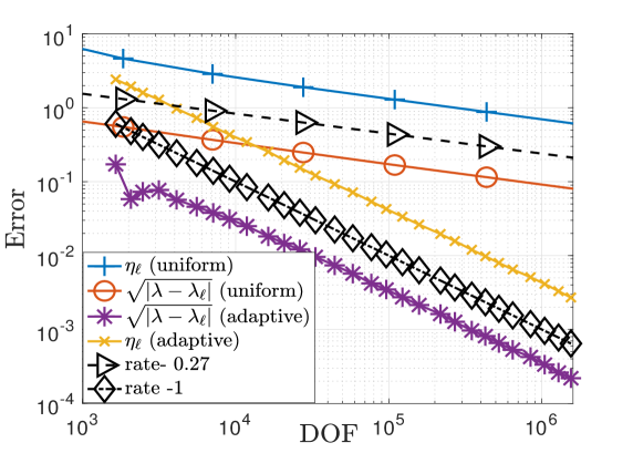
Figure 5.1: Convergence results for Lshaped-domain

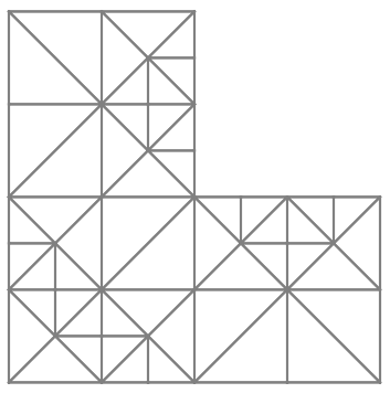
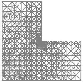
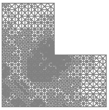
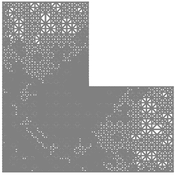
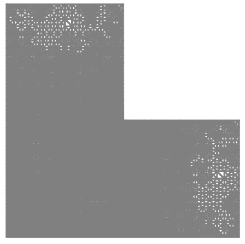
Figure 5.2: Adaptively refined meshes for Lshaped-domain with 5.2 151, DOF, 5.2 5571 DOF, 5.2 11836DOF, 5.2 26286 DOF, and 5.2 58291 DOF.

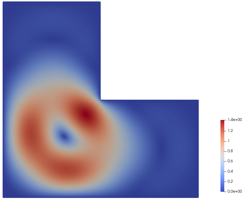
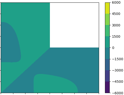
Figure 5.3: 5.3 Velocity profile, 5.3 Pressure profile,

5.2 Slit-domain

In this illustration, we address the resolution of the Stokes eigenvalue problem (2.1) within the Slit-domain, denoted as $\Omega=(0,1)^{2}\setminus[0,1]$. The established benchmark for the primary eigenvalue is $\lambda=29.9168629$, as documented in [21]. The error profile for the first eigenvalue is depicted in Figure 5.4. Notably, the decay of the error, expressed as $\sqrt{|\lambda-\lambda_{\ell}|}$ between the discrete eigenvalue and the referenced first eigenvalue, follows a rate of approximately $0.25$ with a uniformly refined mesh. Figure 5.4 illustrates that the slope of the eigenvalue error aligns with that of the estimator $\eta_{\ell}$, signifying the reliability and efficiency of our estimator. Simultaneously, utilizing an adaptively refined mesh results in an error decay rate of about $1$ for $\sqrt{|\lambda-\lambda_{\ell}|}$. The velocity and pressure profiles are showcased in Figure 5.6, while Figure 5.5 displays a sequence of adaptively refined meshes at different levels. These mesh depictions reveal substantial refinements near the singularity, confirming the anticipated effectiveness of our adaptive scheme.

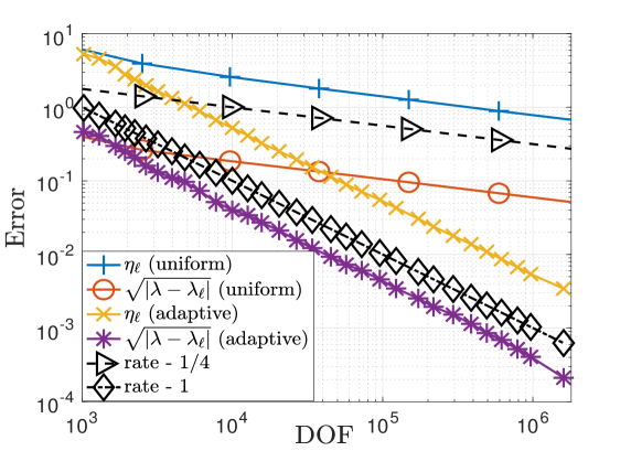
Figure 5.4: Convergence results for Slit-domain

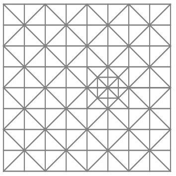
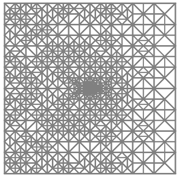
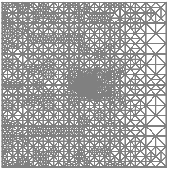
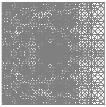
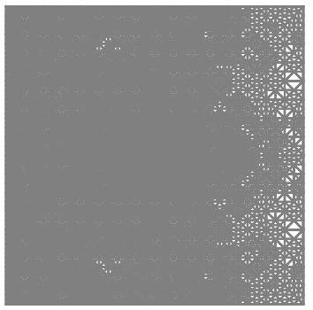
Figure 5.5: Adaptively refined meshes for Lshaped-domain with 5.5 679, DOF, 5.5 6047 DOF, 5.5 12636 DOF, 5.5 26718 DOF, and 5.5 57140 DOF.

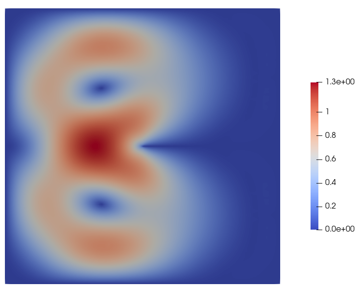
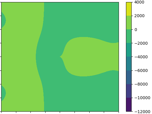
Figure 5.6: 5.6 Velocity profile, 5.6 Pressure profile.

5.3 The Fichera corner

In this example, we address the Stokes eigenvalue problem (2.1) in the context of the Fichera corner, represented as $\Omega=\Omega_{1}\setminus\bar{\Omega}_{2}$, where $\Omega_{1}=(0,0.8)\times(0.0,1)\times(0.0,1.2)$ and $\Omega_{2}=(0.0,0.4)\times(0.0,0.5)\times(0.0,0.6)$. For this particular example, we designate $\theta$ as $0.1$. The graphical representation in Figure 5.7 demonstrates that the estimator $\eta_{\ell}$ exhibits a decay rate of approximately $2/3$ when utilizing adaptive meshes. Figure 5.8 presents the velocity and pressure profiles, while Figure 5.85.8 showcases the adaptively refined mesh containing $1009839$ degrees of freedom (DOFs). These mesh visualizations highlight significant refinements in proximity to the singularity, affirming the numerical effectiveness of our adaptive scheme.

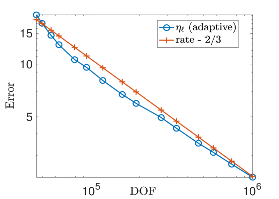
Figure 5.7: Convergence results for the Fichera corner

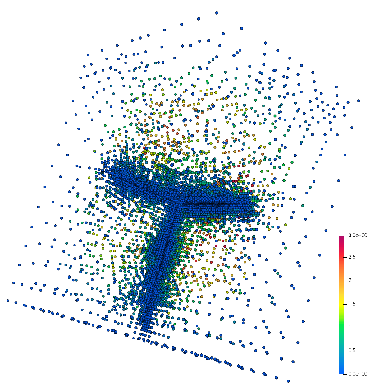
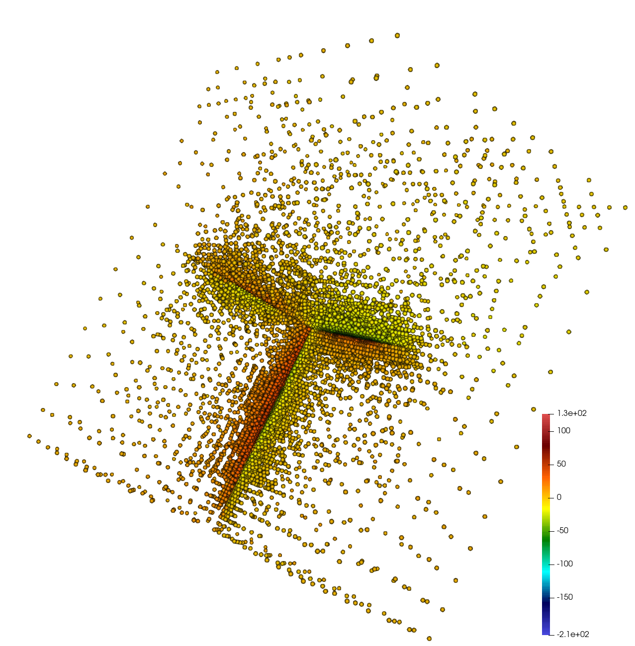
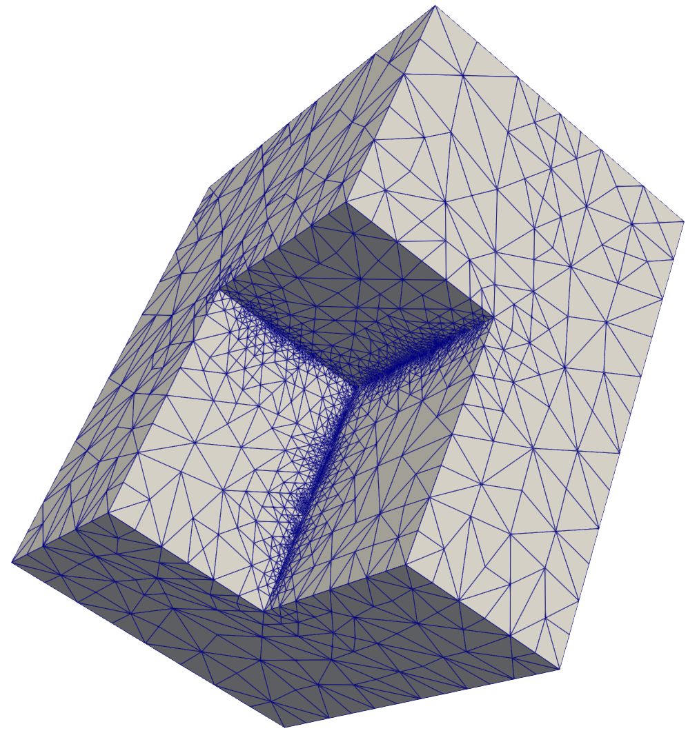
Figure 5.8: 5.8 Velocity profile, 5.8 Pressure profile, 5.8 Adaptively refined meshes for the Fichera corner with 1009839 DOFs.

Conclusion

This paper addressed the application of adaptive mixed FEM to Stokes eigenvalue problems. We achieved the following key results:

• Rate optimality: Established the optimal convergence rate for Algorithm 1, demonstrating its efficiency in approximating eigenvalues.

• Novel estimator: Proposed a new estimator specifically tailored for Stokes eigenvalue problems. This estimator exhibits local equivalence to the established work of Lovadina et al. [25].

• Theoretical rigor: Provided rigorous proofs for quasi-orthogonality and discrete reliability, solidifying the theoretical foundation of our approach.

• Numerical validation: Confirmed the optimality result through computational experiments, showcasing the practical effectiveness of our method.

These findings contribute significantly to the field of adaptive FEM for eigenvalue problems, offering a robust and efficient framework for tackling Stokes eigenvalue analysis.

References

- [1] M. Ainsworth and J. T. Oden, A posteriori error estimation in finite element analysis, Computer methods in applied mechanics and engineering, 142 (1997), pp. 1–88.
- [2] M. S. Alnaes, J. Blechta, J. Hake, A. Johansson, B. Kehlet, A. Logg, C. N. Richardson, J. Ring, M. E. Rognes, and G. N. Wells, The FEniCS project version 1.5, Archive of Numerical Software, 3 (2015).
- [3] I. Babuška and J. E. Osborn, Finite element-galerkin approximation of the eigenvalues and eigenvectors of selfadjoint problems, Mathematics of computation, 52 (1989), pp. 275–297.
- [4] E. Bänsch, P. Morin, and R. H. Nochetto, An adaptive uzawa fem for the stokes problem: Convergence without the inf-sup condition, SIAM Journal on Numerical Analysis, 40 (2002), pp. 1207–1229.
- [5] P. Binev, W. Dahmen, and R. DeVore, Adaptive finite element methods with convergence rates, Numer. Math., 97 (2004), pp. 219–268.
- [6] D. Boffi, Stability of higher order triangular hood-taylor methods for the stationary stokes equations, Mathematical Models and Methods in Applied Sciences, 4 (1994), pp. 223–235.
- [7] , Three-dimensional finite element methods for the stokes problem, SIAM Journal on Numerical Analysis, 34 (1997), pp. 664–670.
- [8] , Finite element approximation of eigenvalue problems, Acta Numerica, 19 (2010), pp. 1–120.
- [9] D. Boffi, F. Brezzi, and M. Fortin, Mixed finite element methods and applications, vol. 44 of Springer Series in Computational Mathematics, Springer, Heidelberg, 2013.
- [10] D. Boffi, F. Brezzi, and L. Gastaldi, On the convergence of eigenvalues for mixed formulations, Ann. Scuola Norm. Sup. Pisa Cl. Sci. (4), 25 (1997), pp. 131–154 (1998). Dedicated to Ennio De Giorgi.
- [11] D. Boffi, D. Gallistl, F. Gardini, and L. Gastaldi, Optimal convergence of adaptive fem for eigenvalue clusters in mixed form, Mathematics of Computation, 86 (2017), pp. 2213–2237.
- [12] D. Boffi and L. Gastaldi, Adaptive finite element method for the maxwell eigenvalue problem, SIAM Journal on Numerical Analysis, 57 (2019), pp. 478–494.
- [13] C. Carstensen, M. Feischl, M. Page, and D. Praetorius, Axioms of adaptivity, Computers & Mathematics with Applications, 67 (2014), pp. 1195–1253.
- [14] J. M. Cascon, C. Kreuzer, R. H. Nochetto, and K. G. Siebert, Quasi-optimal convergence rate for an adaptive finite element method, SIAM Journal on Numerical Analysis, 46 (2008), pp. 2524–2550.
- [15] X. Dai, J. Xu, and A. Zhou, Convergence and optimal complexity of adaptive finite element eigenvalue computations, Numerische Mathematik, 110 (2008), pp. 313–355.
- [16] W. Dörfler, A convergent adaptive algorithm for poisson?s equation, SIAM Journal on Numerical Analysis, 33 (1996), pp. 1106–1124.
- [17] M. Feischl, Optimality of a standard adaptive finite element method for the stokes problem, SIAM Journal on Numerical Analysis, 57 (2019), pp. 1124–1157.
- [18] , Inf-sup stability implies quasi-orthogonality, Mathematics of Computation, 91 (2022), pp. 2059–2094.
- [19] T. Gantumur, On the convergence theory of adaptive mixed finite element methods for the stokes problem, arXiv preprint arXiv:1403.0895, (2014).
- [20] J. Gedicke and A. Khan, Arnold–winther mixed finite elements for stokes eigenvalue problems, SIAM Journal on Scientific Computing, 40 (2018), pp. A3449–A3469.
- [21] , Divergence-conforming discontinuous galerkin finite elements for stokes eigenvalue problems, Numerische Mathematik, 144 (2020), pp. 585–614.
- [22] J. Han, Z. Zhang, and Y. Yang, A new adaptive mixed finite element method based on residual type a posterior error estimates for the stokes eigenvalue problem, Numerical Methods for Partial Differential Equations, 31 (2015), pp. 31–53.
- [23] P. Huang, Lower and upper bounds of stokes eigenvalue problem based on stabilized finite element methods, Calcolo, 52 (2015), pp. 109–121.
- [24] H. Liu, W. Gong, S. Wang, and N. Yan, Superconvergence and a posteriori error estimates for the stokes eigenvalue problems, BIT Numerical Mathematics, 53 (2013), pp. 665–687.
- [25] C. Lovadina, M. Lyly, and R. Stenberg, A posteriori estimates for the stokes eigenvalue problem, Numerical Methods for Partial Differential Equations: An International Journal, 25 (2009), pp. 244–257.
- [26] K.-A. Mardal and J. B. Haga, Block preconditioning of systems of PDEs, in Automated Solution of Differential Equations by the Finite Element Method: The FEniCS Book, A. Logg, K.-A. Mardal, and G. Wells, eds., Springer Berlin Heidelberg, Berlin, Heidelberg, 2012, pp. 643–655.
- [27] P. Morin, K. G. Siebert, and A. Veeser, A basic convergence result for conforming adaptive finite elements, Mathematical Models and Methods in Applied Sciences, 18 (2008), pp. 707–737.
- [28] R. Verfürth, Error estimates for a mixed finite element approximation of the stokes equations, RAIRO. Analyse numérique, 18 (1984), pp. 175–182.
- [29] , A posteriori error estimation techniques for finite element methods, OUP Oxford, 2013.