Quantum Generative Diffusion Model

Abstract

This paper introduces the Quantum Generative Diffusion Model (QGDM), a fully quantum-mechanical model for generating quantum state ensembles, inspired by Denoising Diffusion Probabilistic Models. QGDM features a diffusion process that introduces timestep-dependent noise into quantum states, paired with a denoising mechanism trained to reverse this contamination. This model efficiently evolves a completely mixed state into a target quantum state post-training. Our comparative analysis with Quantum Generative Adversarial Networks demonstrates QGDM’s superiority, with fidelity metrics exceeding 0.99 in numerical simulations involving up to 4 qubits. Additionally, we present a Resource-Efficient version of QGDM (RE-QGDM), which minimizes the need for auxiliary qubits while maintaining impressive generative capabilities for tasks involving up to 8 qubits. These results showcase the proposed models’ potential for tackling challenging quantum generation problems.

I Introduction

Generative models have attracted widespread attention and achieved significant success in academic and industrial spheres [1, 2]. These models have demonstrated exceptional capabilities in various tasks, particularly in the generation of high-quality data. Notably, in the past two years, large models such as ChatGPT and Stable Diffusion have shown extraordinary performance and creativity in the fields of human-machine dialogue and image generation[3, 4]. These generative models have not only achieved technological breakthroughs but have also had a profound impact on everyday life[5]. The core goal of generative models is to learn the underlying probability distributions from a given dataset. Once trained, these models can generate new data that are similar to the distribution of the training samples, demonstrating their understanding and mastery of the underlying patterns in the data.

In the surge of interest in generative models, quantum generative models[6], as the quantum counterparts of classical generative models in the field of quantum machine learning[7, 8, 9, 10, 11], have sparked great interest in the academic community. Quantum generative models combine the advantages of quantum computing and offer new possibilities for data generation. So far, there have been several preliminary explorations of various quantum generative models, including Quantum Generative Adversarial Network (QGAN) [12, 13, 14], Quantum Circuit Born Machine (QCBM) [15, 16], Quantum Variational Autoencoder (QVAE) [17], and Quantum Boltzmann Machine (QBM) [18]. Among them, QGAN, the quantum counterpart of the classical Generative Adversarial Network (GAN) [19], has received considerable attention for its remarkable applications, including but not limited to generating quantum state ensembles [13, 20, 21], image generation [22, 23, 24], and fitting classical discrete distributions [14, 25, 26]. QGAN provides a pathway for researchers to more effectively simulate and explore complex quantum systems, especially in generating and processing data related to quantum states.

I-A Motivations

Although QGANs are applied in various fields, they inherit challenges in convergence from their classical counterparts [27, 21]. Furthermore, QGAN face distinct challenges in the quantum realm, such as difficulties in achieving convergence for tasks like generating mixed quantum states [27]. These challenges not only make training QGAN difficult but also limit their broader application in critical quantum state generation tasks. These limitations highlight the need for more effective alternatives to address these complex quantum state generation tasks.

In pursuit of this objective, it is imperative to explore the quantum analogs of classical diffusion models [28, 29, 30, 31]. Classical diffusion models have been proven to have superior generative performance in many fields compared to GAN, and they possess friendly convergence properties [32, 33]. Following the diffusion models in the classical domain, which emerged as strong alternatives to traditional GAN, quantum versions of diffusion models are expected to offer similar benefits, including more stable training processes and superior generative capabilities. The development of quantum analogues of classical diffusion models holds promise for addressing some of the current challenges in QGAN and could contribute significantly to the advancement of the field of quantum generative learning. This marks an important step in harnessing the potential of quantum technology in generative models. Therefore, motivated by these considerations, this paper embarks on exploring quantum analogues of classical diffusion models, aiming to leverage their potential in enhancing quantum generative learning.

I-B Contributions

Inspired by classical diffusion models, this paper introduces a novel quantum generative model: the Quantum Generative Diffusion Model (QGDM), for quantum state generation tasks. Our objectives are to define a timestep-dependent diffusion process, design an efficient quantum state denoising process, and benchmark our model against other quantum generative models in pure and mixed state generation tasks. Our contributions are summarized as follows:

1. We propose the Quantum Generative Diffusion Model (QGDM) for generating quantum states. Similar to classical diffusion models, QGDM consists of two independent processes: a diffusion process using depolarizing channels and a denoising process using a parameterized model. Once trained, the QGDM can take a completely mixed state as input and accurately reconstruct the target quantum state.

2. We employ depolarizing channels to model the diffusion process of the QGDM, effectively replicating physical phenomena. Additionally, we provide a detailed mathematical framework to describe the transition from an initial state to a quantum state at any given timestep, thereby improving our ability to sample noisy quantum states more effectively.

3. We design the circuit details for the denoising process, which include timestep embedding circuit and denoising circuit. We also discuss the deeper reasons behind such a design to inspire future work in similar fields. This includes timestep-related quantum machine learning models and other quantum analogues of diffusion models.

4. To reduce the number of auxiliary qubits required during the denoising process, we introduce a Resource-Efficient version of QGDM: Resource-Efficient QGDM (RE-QGDM), thus enhancing the model’s efficiency in addressing more complex, large-scale problems.

The remainder of this article is structured as follows. Initially, in Section II, we delve into the existing literature and the foundational work relevant to quantum generative models. Subsequently, in Section III, we present an in-depth exposition of our innovative Quantum Generative Diffusion Model (QGDM) framework. Further, Section IV is dedicated to introducing a Resource-Efficient iteration of the QGDM (RE-QGDM). Section V analyzes the rationale behind the design of the denoising process and presents simulation results to support these insights. These analyses and simulation outcomes are poised to aid future research in similar models. The numerical simulations setup and comparative results with other quantum generative model are shown in Section VI. Finally, Section VII concludes this article. The notations are summarized in Table I.

TABLE I: Notations

Notation	Description
$t$	Timestep
$T$	Total Timesteps of the Diffusion Process
$|\psi\rangle$	Quantum State
$\rho$	Density Matrix of A Quantum System
$\rho_{0}$	Target Quantum State
$\rho_{t}$	System’s Density Matrix at Timestep $t$
$\rho_{T}$	Completely Mixed State
$\tau_{t}$	Timestep Embedding Quantum State
$\mathbb{I}$	Identity Matrix
$\beta_{t}$	Noise Parameter Dependent on $t$
$\alpha_{t}$	Noise Parameter Dependent on $t$, $\alpha_{t}=1-\beta_{t}$
$\bar{\alpha}_{t}$	Accumulated Noise Parameter $\bar{\alpha}_{t}=\prod_{i}^{t}{\alpha_{i}}$
$\mathcal{E}(\cdot,\cdot)$	Diffusion Process Function
$f_{\boldsymbol{\Theta}}(\cdot,\cdot)$	Denoising Process Function Parameterized by $\boldsymbol{\Theta}$
$\mathcal{T}(\boldsymbol{\omega},\cdot)$	Timestep Embedding Circuit Parameterized by $\boldsymbol{\omega}$
$U(\boldsymbol{\theta})$	Denoising Circuit Parameterized by $\boldsymbol{\theta}$
$\text{tr}(\cdot)$	Trace Operation
$\text{tr}_{B}(\cdot)$	Partial Trace Operation over Subsystem B
$F(\cdot,\cdot)$	Quantum Fidelity Function
$N$	Number of Qubits in the Target State
$N_{\text{time}}$	Number of Qubits in the Time Encoding circuit
$d$	Dimension of the Hilbert Space of the System
$\lambda$	Hyperparameter in Loss Function
$A^{\dagger}$	Hermitian Conjugate of the Operator $A$
$\mathcal{L}_{t}$	Loss Function at Timestep $t$
$\mathcal{L}$	Total Loss Function

II Related Works

Quantum generative models, a pivotal sector in quantum machine learning, encompass various models including Quantum Circuit Born Machine (QCBM) [15], Quantum Boltzmann Machine (QBM) [18], Quantum Variational Autoencoder (QVAE) [17], and Quantum Generative Adversarial Network (QGAN) [12, 13].

The Quantum Circuit Born Machine (QCBM) uses quantum circuits to generate classical bit-strings from specific probability distributions, a concept first proposed by Benedetti et al. [15]. This model has seen substantial advances [16, 34, 35, 36], finding applications in various fields including Monte Carlo simulations[37], financial data generation[38, 39], and joint distribution learning[38, 40]. The Quantum Boltzmann Machine (QBM), functioning as a quantum counterpart to the classical Boltzmann Machine [41, 42], QBM utilizes quantum device to prepare Boltzmann distributions, by replacing the units in the classical Boltzmann Machine with qubits and substituting the energy function with a parameterized Hamiltonian. QBM was first demonstrated by Amin et al. [18], leading to significant model enhancements[43, 44, 45]. Khoshaman et al.[17] introduced the Quantum Variational Autoencoder (QVAE), using the QBM as a prior in Discrete VAE[46], with subsequent developments including annealer-based[47] and gate-based QVAE[48]. In the realm of QGANs, Lloyd and Weedbrook [12] developed a comprehensive taxonomy, classifying them by the quantum or classical nature of their components. This was empirically supported by Dallaire-Demers and Killoran [13], who demonstrated the efficacy of QGAN in generating the desired quantum data. The field has since explored applications in quantum states generation [49, 20, 27, 21], image generation[22, 23, 24], and discrete data generation[14, 25, 26]. For an in-depth review of these quantum generative models, refer to the comprehensive work by Tian et al.[6].

During our research, several papers [50, 51, 52] concurrently proposed quantum analogs to the classical diffusion model. Ref. [50] introduces several implementation strategies for the quantum version of diffusion models, along with theoretical tools that could be applicable. However, it mainly focuses on conceptual aspects and lacks detailed implementations or experimental validations. In contrast, our work introduces a comprehensive concept and delves into technical details, including comparisons with other quantum generative models. Ref. [51] proposes the QuDDPM algorithms, which generate individual pure states from a target distribution. This approach is distinct from achieving the goal of generating a quantum state ensemble, an objective considered in other quantum generative models papers such as Refs. [13, 20, 27, 21], as well as in our work. To the best of the authors’ knowledge, generating quantum state ensembles is crucial for studies including, but not limited to, the properties of quantum states [53, 54, 55], quantum simulation [56], and quantum information theory [57]. Ref. [52] uses a classical approach for the diffusion process, while the denoising process is performed using a trainable quantum circuit to accomplish the denoising task. However, our method is fully quantum mechanical, encompassing both the noise addition and denoising processes of the quantum state.

III Quantum Generative Diffusion Model

III-A General Framework

Figure 1: The framework of the proposed Quantum Generative Diffusion Model (QGDM).

The Quantum Generative Diffusion Model (QGDM) adheres to a general framework, as illustrated in Fig. 1. Analogous to classical diffusion models, QGDM encompasses a forward (diffusion) process $\mathcal{E}(\rho_{t-1},t)$ and a backward (denoising) process $f_{\boldsymbol{\Theta}}(\rho_{t},t)$. The diffusion process $\mathcal{E}(\rho_{t-1},t)$ takes a $N$ qubits quantum state $\rho_{t-1}$ and timestep $t$ as inputs, producing a quantum state $\rho_{t}$ with increased noise. In our methodology, $\mathcal{E}(\rho_{t-1},t)$ is modeled as a depolarizing channel. When $t=0$, $\rho_{0}$ represents the target quantum state. Conversely, at $t=T$, $\rho_{T}$ transforms into a completely mixed state, expressed as $\mathbb{I}/2^{N}$. The denoising process employs a model $f_{\boldsymbol{\Theta}}(\rho_{t},t)$ with trainable parameters $\boldsymbol{\Theta}$, which denoises the noisy input quantum state $\rho_{t}$, producing a cleaner quantum state $\rho_{t-1}$. After applying the function $f_{\boldsymbol{\Theta}}(\cdot,\cdot)$ $T$ times to $\rho_{T}$, the target quantum state $\rho_{0}$ is recovered.

III-B Forward

In the natural world, diffusion is governed by non-equilibrium thermodynamics, driving systems toward equilibrium [58]. As a system undergoes evolution, its entropy increases until it reaches maximum entropy at equilibrium, indicating no further evolution. In quantum information theory, the depolarizing channel is considered a ”worst-case scenario” [59]. Under its influence, a quantum state $\rho$ gradually degrades, eventually transforming into a completely mixed state. This state is characterized by the highest entropy, representing the pinnacle of randomness in quantum systems.

A completely mixed state of $N$ qubits is mathematically represented as $\mathbb{I}/{2^{N}}=\sum\limits_{i}{\frac{1}{{{2^{N}}}}}\left|i\right\rangle\left\langle i\right|$. This denotes that each computational basis state $\left|i\right\rangle$ occurs with an equal probability of $\frac{1}{2^{N}}$. This uniform probability distribution across all computational bases renders the state maximally random, similar to the uniform distribution in classical data. At timestep $t$, the diffusion process of QGDM adds depolarizing noise to an $N$ qubits quantum state $\rho_{t-1}$:

$$\rho_{t} =\mathcal{E}\left(\rho_{t-1},t\right)$$ (1)

$$=\beta_{t}\mathbb{I}/d+(1-\beta_{t})\rho_{t-1},$$

where $d=2^{N}$ denotes the dimension of Hilbert space and $\beta_{t}\in[0,1]$ is a timestep-dependent scalar. Equation (1) indicates that the input quantum state $\rho_{t-1}$ persists unchanged with a probability of $1-\beta_{t}$. Conversely, it is replaced by the completely mixed state $\mathbb{I}/d$ with a probability of $\beta_{t}$. This indicates the loss of original information in the quantum system. By setting an appropriate sequence of $\beta_{t}$, a series of depolarizing channel sequences acting on the quantum state $\rho_{0}$ will eventually yield the output $\rho_{T}\approx\mathbb{I}/d$.

III-B1 Efficient Quantum State Transition to Arbitrary Timestep

Equation (1) mathematically describes a single-step diffusion process. Sequentially applying this process allows for the generation of quantum states $\rho_{t}$ at any given timestep between 1 and $T$. However, repeatedly applying $\mathcal{E}$ to obtain a specific timestep’s quantum state $\rho_{t}$ is inefficient.

To enhance the efficiency of transition from the initial state $\rho_{0}$ to a specific state $\rho_{t}$, we introduce a novel parameter $\alpha_{t}=1-\beta_{t}$. Consequently, Equation (1) can be reformulated as follows:

$$\rho_{t} =\mathcal{E}\left(\rho_{t-1},t\right)$$ (2)

$$=(1-\alpha_{t})\mathbb{I}/d+\alpha_{t}\rho_{t-1}.$$

Thus we have:

Theorem 1: For any $t\in[1,T]$, the relationship between $\rho_{0}$ and $\rho_{t}$ can be described by:

$$\rho_{t}=\left(1-\bar{\alpha}_{\mathrm{t}}\right)\mathbb{I}/d+\bar{\alpha}_{\mathrm{t}}\rho_{0},$$ (3)

where $\bar{\alpha}_{\mathrm{t}}=\prod\limits_{i=1}^{t}\alpha_{i}$.
Proof:

$$\rho_{t} =\left(1-\alpha_{t}\right)\mathbb{I}/d+\alpha_{t}\rho_{t-1}$$ (4)

$$=\left(1-\alpha_{t}\right)\mathbb{I}/d+\alpha_{t}\left[\left(1-\alpha_{t-1}\right)\mathbb{I}/d+\alpha_{t-1}\rho_{t-2}\right]$$

$$=\left(1-\alpha_{t}\alpha_{t-1}\right)\mathbb{I}/d+\alpha_{t}\alpha_{t-1}\rho_{t-2}$$

$$=\left(1-\alpha_{t}\alpha_{t-1}\right)\mathbb{I}/d$$

$$\quad+\alpha_{t}\alpha_{t-1}\left[\left(1-\alpha_{t-2}\right)\mathbb{I}/d+\alpha_{t-2}\rho_{t-3}\right]$$

$$=\left(1-\alpha_{t}\alpha_{t-1}\alpha_{t-2}\right)\mathbb{I}/d+\alpha_{t}\alpha_{t-1}\alpha_{t-2}\rho_{t-3}$$

$$=\ldots$$

$$=\left(1-\prod\limits_{i=1}^{t}\alpha_{i}\right)\mathbb{I}/d+\prod\limits_{i=1}^{t}\alpha_{i}\rho_{0}$$

$$=\left(1-\bar{\alpha}_{\mathrm{t}}\right)\mathbb{I}/d+\bar{\alpha}_{\mathrm{t}}\rho_{0}.$$

Thus, Eq. (3) enables the direct transition from $\rho_{0}$ to a quantum state $\rho_{t}$ in any chosen timestep.

III-B2 Noise Schedule

The noise parameter ${\beta_{t}}$ determines the rate at which the target state $\rho_{0}$ approaches the completely mixed state $\rho_{T}$. ${\beta_{t}}$ influences the learning difficulty of the denoising process, ultimately affecting the model’s generative performance. Furthermore, the selection of ${\beta_{t}}$ must satisfy two conditions:

$$\left\{\begin{array}[]{l}{\beta_{t}}\in\left[{0,1}\right],\forall t\\ {{\cal E}}(\dots{\cal E}({{\cal E}}({\rho_{0};1});2)\dots;T)\approx\mathbb{I}/d.\end{array}\right.$$ (5)

Since the depolarizing channel is similar to the reparameterization trick[60], we refer to the cosine noise schedule used in the classical diffusion model paper[31] for selecting $\beta_{t}$:

$$\beta_{t}=1-\frac{\bar{\alpha}t}{\bar{\alpha}{t-1}},$$ (6)

where

$$\bar{\alpha}_{t}=\frac{g(t)}{g(0)},\quad g(t)=\cos\left(\frac{t/T+s}{1+s}\cdot\frac{\pi}{2}\right)^{2},$$ (7)

with $s$ being a small offset hyperparameter. We note that there are other noise schedules, such as the linear noise schedule [29] and learned noise schedule [61]. Exploring other noise schedule’s impacts on QGDM’s generative performance, or designing specific noise schedules for QGDM, is an interesting research direction, which we leave for future work.

III-C Backward

The primary objective of the backward process in the Quantum Generative Diffusion Model (QGDM) is to restore the target quantum state $\rho_{0}$ from the completely mixed state $\rho_{T}$. In designing the parameterized quantum operation $f_{\boldsymbol{\Theta}}(\rho_{t},t)$ for denoising, two key aspects are vital. Firstly, considering the diffusion process is modeled via a depolarizing channel, the denoising function $f$ essentially serves as the reverse of this process. Given the non-unitary nature of the diffusion process, it is critical for the transformation $f$ to also manifest non-unitary characteristics. Secondly, the denoising function $f$ assumes varied roles at different timesteps. For example, at the final timestep $t=T$, $f$ should convert a completely mixed state into a less noisy quantum state, though still somewhat mixed. Conversely, at $t=1$, $f$ aims to produce a completely noise-free quantum state, $\rho_{0}$. This implies the necessity for $T$ distinct denoising functions, each with its own set of trainable parameters $\boldsymbol{\Theta}$, to fulfill each specific task. To optimize parameter management in QGDM, the timestep $t$ is incorporated into the input. This integration is crucial for shaping the function $f_{\boldsymbol{\Theta}}(\rho_{t},t)$, as it allows the model to effectively utilize temporal dynamics to accurately estimate $\rho_{t-1}$. Such an approach strikes a balance between model complexity and computational efficiency.

Our design for the denoising process $f_{\boldsymbol{\Theta}}(\rho_{t},t)$ is illustrated in Fig. 2. $f_{\boldsymbol{\Theta}}(\rho_{t},t)$ comprises two modules: a timestep embedding circuit $\mathcal{T}(\boldsymbol{\omega},t^{\prime})$ parameterized by $\boldsymbol{\omega}$, and a denoising circuit $U(\boldsymbol{\theta})$ parameterized by $\boldsymbol{\theta}$, thus $\boldsymbol{\Theta}=\{\boldsymbol{\omega},\boldsymbol{\theta}\}$. A timestep embedding circuit $\mathcal{T}(\boldsymbol{\omega},t^{\prime})$, operating on an auxiliary register with $N_{\text{time}}$ qubits, is utilized to produce the state $\tau_{t}$. Here, $t^{\prime}=t\pi/T$ represents a normalized mapping of the timestep $t$, scaling its range from 0 to $\pi$. Subsequently, the composite system of the timestep embedding state $\tau_{t}$ and the input state $\rho_{t}$ is fed into the denoising circuit $U({\boldsymbol{\theta}})$. Afterward, all qubits are regrouped into two registers: register A with $N$ qubits and register B with $N_{\text{time}}$ qubits. Finally, register B is traced out to yield the predicted denoised quantum state $\tilde{\rho}_{t-1}$.

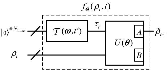
Figure 2: The denoising process framework, $f_{\boldsymbol{\Theta}}(\rho_{t},t)$, is composed of a timestep embedding circuit $\mathcal{T}(\boldsymbol{\omega},t^{\prime})$ and a denoising circuit $U(\boldsymbol{\theta})$, where $\boldsymbol{\Theta}=\{\boldsymbol{\omega},\boldsymbol{\theta}\}$. The timestep embedding circuit $\mathcal{T}(\boldsymbol{\omega},t^{\prime})$ acts on $N_{\text{time}}$ qubits initialized in the zero state to generate a quantum state $\tau_{t}$ containing temporal information, where $\boldsymbol{\omega}$ are the trainable parameters of $\mathcal{T}$, and $t^{\prime}=t\pi/T$ is a scalar mapping the timestep $t$ to the range [0, $\pi$]. The denoising circuit $U(\boldsymbol{\theta})$, parameterized by trainable parameters $\boldsymbol{\theta}$, acts on the composite system $\tau_{t}\otimes\rho_{t}$ and regroups the output qubits into a register A with $N$ qubits and a register B with $N_{\text{time}}$ qubits. The predicted quantum state $\tilde{\rho}_{t-1}$ in timestep $t-1$ is obtained by tracing out register B.

III-C1 Timestep Embedding Circuit

In $f_{\boldsymbol{\Theta}}(\rho_{t},t)$, which receives timestep $t$ and quantum state $\rho_{t}$ as inputs, a critical consideration is how to encode the temporal information $t$ into the quantum state. This is a classical-to-quantum encoding challenge, where methods such as qubit encoding [62, 63, 64] or amplitude encoding [65] could be employed to embed $t$ into a quantum system. In this work, we utilize the quantum embedding method [12] to obtain the timestep embedding state $\tau_{t}$. This technique employs additional rotation gates with trainable parameters, enabling the embedding of classical data into an appropriate position of the Hilbert space. When the trainable parameters of the additional rotation gates are set to zero, this method reduces to the qubit encoding method. Hence, the quantum embedding method offers greater capabilities than the qubit encoding method.

We use a timestep embedding circuit $\mathcal{T}$ with $N_{\text{time}}$ qubits to encode temporal information into a quantum state:

$$\tau_{t}=\mathcal{T}(\boldsymbol{\omega},t^{\prime})\left(\left|{\rm{0}}\right\rangle{\left\langle{\rm{0}}\right|}\right)^{\otimes N_{\text{time}}}\mathcal{T}^{\dagger}(\boldsymbol{\omega},t^{\prime}),$$ (8)

where $t^{\prime}=t\pi/T$ is a scalar mapping the timestep $t$ to the range [0, $\pi$], and $\boldsymbol{\omega}$ are the trainable parameters of $\mathcal{T}$. The structure of a 4 qubits timestep embedding circuit is shown in Fig. 3. As observed, the timestep embedding circuit is a multi-layer stacked structure with $L_{\mathcal{T}}$ layers of repeating circuits.

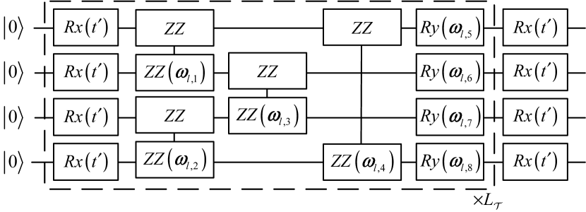
Figure 3: Architecture of the timestep embedding circuit with $\boldsymbol{\omega}$ as the trainable parameters of $\mathcal{T}$, and $t^{\prime}=t\pi/T$. The circuit includes single-qubit gates $Rx$ and $Ry$, and a two-qubit gate $ZZ(\phi)=\exp{(-i\phi(Z\otimes Z)/2)}$. To enhance the learning capability of the circuit, the part enclosed by the dashed lines is repeated $L_{\mathcal{T}}$ times.

III-C2 Denoising Circuit

The denoising circuit $U(\boldsymbol{\theta})$ acts on the composite system $\tau_{t}\otimes\rho_{t}$. Subsequently, all qubits are regrouped into subsystems A and B, where they possess $N$ and $N_{\text{time}}$ qubits, respectively. By tracing out subsystem B, we obtain the predicted output $\tilde{\rho}_{t-1}$:

$${{{\tilde{\rho}}_{{\rm{t}}-1}}} =f_{\boldsymbol{\Theta}}(\rho_{t},t)$$ (9)

$$=\text{tr}_{\text{B}}\left(U(\theta)\left(\tau_{t}\otimes\rho_{t}\right)U^{\dagger}(\theta)\right).$$

In our proposed design, subsystem A is explicitly engineered to generate the model-predicted denoised quantum state ${\tilde{\rho}}_{t-1}$, a task markedly different from that of subsystem B, which is designated for the input of $\rho_{t}$. This design requires register A to assimilate information from $\rho_{t}$ and synergize it with information from $\tau_{t}$. Initially, using register B to output ${\tilde{\rho}}_{t-1}$ might seem intuitive. However, this approach is eschewed due to its propensity to cause model failure. This failure stems from the minimal discrepancy between $\rho_{t}$ and the ground truth $\rho_{t-1}$, leading to a training challenge where the optimizer, instead of learning to generate the desired output, tends to trivially replicate its input. This phenomenon and its implications are thoroughly examined in Section V, complemented by a numerical simulation to illustrate the concept.

The architecture of a 4 qubits denoising circuit $U(\boldsymbol{\theta})$ is shown in Fig. 4. Such circuit architecture is characterized by the use of $\mathcal{O}(N^{2})$ two-qubit gates, an aspect that may compromise its efficiency. However, our primary objective in this study is to validate the efficacy of our proposed method. Acknowledging that an inferior circuit design could adversely affect this validation, we employ a sophisticated circuit architecture. This choice, admittedly leading to increased gate complexity, is imperative to isolate the method’s performance from limitations inherent in simpler designs. By doing so, we ensure that our results truly reflect the potential of our method, free from the constraints of suboptimal circuits. Moreover, in our design, the circuit structure used at each timestep $t$ is the same, which may be unnecessary. Circuits designed to adapt their architecture at different timesteps can be used to reduce the total number of gates in the entire QGDM model. We leave the task of designing efficient circuit architectures for QGDM for future work. An effective approach is to use quantum architecture search algorithms [66, 67, 68, 69, 70, 71, 72].

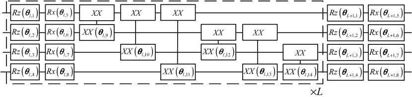
Figure 4: The architecture of a 4 qubits denoising circuit $U(\boldsymbol{\theta})$, where $\boldsymbol{\theta}$ are trainable parameters. The circuit includes single-qubit gates $Rz$ and $Rx$, and a two-qubit gate $XX(\phi)=\exp{(-i\phi(X\otimes X)/2)}$. To enhance the learning capability of the circuit, the part enclosed by the dashed lines is repeated $L$ times.

III-D Training and Generation

The training objective of QGDM is to maximize the quantum fidelity between the predicted $\tilde{\rho}_{t-1}$ and ground truth $\rho_{t-1}$. The loss function is constructed as follows:

$$\min_{\boldsymbol{w},\boldsymbol{\theta}}\mathcal{L}=\mathcal{L}_{0}+\lambda\mathbb{E}_{t\in\text{Uniform}([2,\dots,T])}\left[\mathcal{L}_{t-1}\right],$$ (10)

where $\lambda$ is a hyperparameter used to balance the losses $\mathcal{L}_{0}$ and $\mathbb{E}_{t\in\text{Uniform}([2,\dots,T])}\left[\mathcal{L}_{t-1}\right]$, and we find that setting a small $\lambda$ helps improve the generative effect of QGDM. $\text{Uniform}([2,\dots,T])$ represents a uniform distribution that gives scalar values from 2 to $T$, and $\mathcal{L}_{t}$ is calculated by:

$${\mathcal{L}_{t}}=1-F\left({{\rho_{{\rm{t}}}},{{\tilde{\rho}}_{{\rm{t}}}}}\right),$$ (11)

where ${\tilde{\rho}}_{{\rm{t}}-1}$ is the prediction of $f_{\boldsymbol{\Theta}}(\rho_{t},t)$ for ground truth $\rho_{t-1}$. $F(\cdot,\cdot)$ is the quantum fidelity function [57, 59], used to measure the distance between any two quantum states $\rho$ and $\sigma$:

$$F(\rho,\sigma)=\left(\operatorname{tr}\sqrt{\rho^{1/2}\sigma\rho^{1/2}}\right)^{2}.$$ (12)

The QGDM training algorithm is presented in Algorithm 1. Once the parameters are trained, we can iteratively obtain the target state $\rho_{0}$ from the completely mixed state $\rho_{T}$ using $\boldsymbol{\omega}^{*}$ and $\boldsymbol{\theta}^{*}$. The target quantum state $\rho_{0}$ can be generated using Algorithm 2 after the completion of training.

Algorithm 1 QGDM training algorithm.

1:  Input: Noise schedule parameters $\{\bar{\alpha_{t}}\}_{t=1}^{T}$. Batch size BS. Weight parameter $\lambda$. Number of qubits of the target state $N$. Number of qubits of the timesetp embedding state $N_{\text{time}}$. Total timestep of the diffusion process $T$. Target quantum state $\rho_{0}$. Learning rate $\eta$. Completely mixed state $\mathbb{I}/d$.

2:  $\boldsymbol{\theta}\sim\text{Uniform}(0,\pi)$, $\boldsymbol{\omega}\sim\text{Uniform}(0,\pi)$

3:  repeat

4:     $\rho_{1}\leftarrow\left(1-\bar{\alpha}_{\mathrm{1}}\right)\mathbb{I}/d+\bar{\alpha}_{\mathrm{1}}\rho_{0}$

5:     $t^{\prime}\leftarrow 1\pi/T$

6:     $\tau_{1}\leftarrow\mathcal{T}(\boldsymbol{\omega},t^{\prime})\left(\left|{\rm{0}}\right\rangle{\left\langle{\rm{0}}\right|}\right)^{\otimes N_{\text{time}}}\mathcal{T}^{\dagger}(\boldsymbol{\omega},t^{\prime})$

7:     $\tilde{\rho}_{0}\leftarrow\text{tr}_{\text{B}}\left(U(\boldsymbol{\theta})\left(\tau_{1}\otimes\rho_{1}\right)U^{\dagger}(\boldsymbol{\theta})\right)$

8:     $\mathcal{L}_{0}\leftarrow 1-F(\rho_{0},\tilde{\rho}_{0})$

9:     $\mathcal{L}\leftarrow 0$

10:     for $i$ from 1 to BS do

11:        Sample a unique timestep $t$ from the uniform distribution $\text{Uniform}([2,\dots,T])$

12:        $\rho_{t}\leftarrow\left(1-\bar{\alpha}_{\mathrm{t}}\right)\mathbb{I}/d+\bar{\alpha}_{\mathrm{t}}\rho_{0}$

13:        $t^{\prime}\leftarrow t\pi/T$

14:        $\tau_{t}\leftarrow\mathcal{T}(\boldsymbol{\omega},t^{\prime})\left(\left|{\rm{0}}\right\rangle{\left\langle{\rm{0}}\right|}\right)^{\otimes N_{\text{time}}}\mathcal{T}^{\dagger}(\boldsymbol{\omega},t^{\prime})$

15:        $\tilde{\rho}_{t-1}\leftarrow\text{tr}_{\text{B}}\left(U(\boldsymbol{\theta})\left(\tau_{t}\otimes\rho_{t}\right)U^{\dagger}(\boldsymbol{\theta})\right)$

16:        $\rho_{t-1}\leftarrow\left(1-\bar{\alpha}_{\mathrm{t-1}}\right)\mathbb{I}/d+\bar{\alpha}_{\mathrm{t-1}}\rho_{0}$

17:        $\mathcal{L}\leftarrow\mathcal{L}+1-F\left(\rho_{t-1},\tilde{\rho}_{t-1}\right)$

18:     end for

19:     $\mathcal{L}\leftarrow\mathcal{L}_{0}+\lambda\frac{1}{\textbf{\text{BS}}}\mathcal{L}$

20:     $\boldsymbol{\omega}\leftarrow\boldsymbol{\omega}-\eta\nabla_{\boldsymbol{\omega}}\mathcal{L}$

21:     $\boldsymbol{\theta}\leftarrow\boldsymbol{\theta}-\eta\nabla_{\boldsymbol{\theta}}\mathcal{L}$

22:  until converged

23:  Output: Optimal parameters $\boldsymbol{\omega}^{*},\boldsymbol{\theta}^{*}$

Algorithm 2 QGDM generation algorithm.

1:  Input: Number of qubits of the timesetp embedding state $N_{\text{time}}$. Total timestep of the diffusion process $T$. The optimal parameters $\boldsymbol{\omega}^{*},\boldsymbol{\theta}^{*}$. Completely mixed state $\rho_{T}=\mathbb{I}/d$.

2:  Initialize $\tilde{\rho}$ as completely mixed state: $\tilde{\rho}\leftarrow\rho_{T}$

3:  for $t$ from $T$ to 1 do

4:     $t^{\prime}\leftarrow t\pi/T$

5:     $\tau_{t}\leftarrow\mathcal{T}(\boldsymbol{\omega}^{*},t^{\prime})\left(\left|{\rm{0}}\right\rangle{\left\langle{\rm{0}}\right|}\right)^{\otimes N_{\text{time}}}\mathcal{T}^{\dagger}(\boldsymbol{\omega}^{*},t^{\prime})$

6:     Update the generation state: $\tilde{\rho}\leftarrow\text{tr}_{\text{B}}\left(U(\boldsymbol{\theta}^{*})\left(\tau_{t}\otimes\tilde{\rho}\right)U^{\dagger}(\boldsymbol{\theta}^{*})\right)$ using the previous value of $\tilde{\rho}$.

7:  end for

8:  Output: The final generation state $\tilde{\rho}_{0}=\tilde{\rho}$

IV Resource-Efficient Quantum Generative Diffusion Model (RE-QGDM)

In Section III-C, we described our construction of the denoising process $f_{\boldsymbol{\Theta}}(\rho_{t},t)$. The number of qubits required for such denoising process is $N_{\text{time}}+N$. To reduce the use of auxiliary qubits, we propose a new design for the denoising process $f_{\boldsymbol{\Theta}}(\rho_{t},t)$ in this section.

Figure 5: The denoising process design in Resource-Efficient Quantum Generative Diffusion Models (RE-QGDM) is described as follows. $U_{1}(\boldsymbol{\theta}_{1})$ compresses the information of the input $\rho_{t}$ into the last qubit. We combine the timestep embedding quantum state $\tau_{t}$, obtained from the timestep embedding circuit, with the compressed qubit into a composite system and apply a parameterized quantum circuit $U_{2}(\boldsymbol{\theta}_{2})$. Subsequently, tracing out the last qubit yields the predicted quantum state $\tilde{\rho}_{t-1}$.

In the newly developed Resource-Efficient Quantum Gate Denoising Model (RE-QGDM), only $N+1$ qubits are needed to generate a quantum state of $N$ qubits, enhancing its efficiency in terms of resource utilization. Figure 5 illustrates the denoising process circuit for a target state of 3 qubits using RE-QGDM. Initially, the target state $\rho_{t}$ undergoes compression through a Parameterized Quantum Circuit (PQC) denoted as $U_{1}(\boldsymbol{\theta}_{1})$, where $\boldsymbol{\theta}_{1}$ represents its trainable parameters. This process effectively condenses the information from $\rho_{t}$ into the final qubit. Subsequently, this information-rich qubit is merged with the state $\tau_{t}$, forming a composite system. This system is then processed by another PQC, $U_{2}(\boldsymbol{\theta}_{2})$, which operates on the $N+1$ qubits. Following this, the last qubit of the $N+1$-qubit system is traced out, and the remaining $N$ qubits’ reduced density matrix is obtained as the predicted output state ${\tilde{\rho}}{{\rm{t}}-1}$:

$$\tilde{\rho}_{t-1}={\rm{t}}{{\rm{r}}_{4}}\left[{U_{2}\left({{\boldsymbol{\theta}_{2}}}\right)\left({{\tau_{t}}\otimes\rho_{t}^{{}^{\prime}}}\right){U_{2}^{\dagger}}\left({{\boldsymbol{\theta}_{2}}}\right)}\right],$$ (13)

where the timestep embedding state $\tau_{t}$ is given by Eq. (8) and $\rho_{t}^{{}^{\prime}}$ is calculated by:

$$\rho_{t}^{{}^{\prime}}={\rm{t}}{{\rm{r}}_{12}}\left({U_{1}\left({{\boldsymbol{\theta}_{1}}}\right){\rho_{t}}{U_{1}^{\dagger}}\left({{\boldsymbol{\theta}_{1}}}\right)}\right).$$ (14)

Therefore, the trainable parameters for the denoising process $f_{\boldsymbol{\Theta}}(\rho_{t},t)$ of RE-QGDM are $\boldsymbol{\Theta}=\{\boldsymbol{\omega},\boldsymbol{\theta}_{1},\boldsymbol{\theta}_{2}\}$. Apart from the difference in the denoising process used to generate $\tilde{\rho}_{t-1}$, RE-QGDM and QGDM share the same diffusion process, training algorithm, and generation algorithm.

V Critical Evaluation of Denoising in Quantum Generative Diffusion Models

A straightforward design for the denoising process $f_{\boldsymbol{\Theta}}(\rho_{t},t)$ involves using a trainable circuit $U(\boldsymbol{\theta})$ acting on the extended system $\tau_{t}\otimes\rho_{t}$ and then tracing out the qubits of $\tau_{t}$. However, recalling that the noise added to the quantum state in the diffusion process is negligible, this leads to only a trivial difference in noise between $\rho_{t}$ and $\rho_{t-1}$. Oriented by the goal of minimizing the loss function, the learning algorithm easily adapts the circuit $U(\boldsymbol{\theta})$, creating an output nearly identical to its input, thus reducing training losses. However, this adaptation deviates from the intended purpose of $U(\boldsymbol{\theta})$ in QGDM, as it compromises the model’s effectiveness by failing to fulfill its primary function.

The numerical simulation results illustrating the limitations of this design approach are shown in Fig. 6. Part (a) of the figure displays the decreasing trend of the training loss over epochs. Part (b) details the Hilbert-Schmidt (HS) distance [59] between the input and output states of the circuit $U(\boldsymbol{\theta})$ during training. HS distance, a measure used in quantum information to quantify the dissimilarity between two quantum states, is defined as $D_{\text{HS}}(\rho,\sigma)=\sqrt{\text{tr}[(\rho-\sigma)^{2}]}$. Part (c) of the figure shows the fidelity variation between the QGDM-generated state and the target state, indicating the model’s inability to significantly alter the input state during the generation process. The orange solid line represents the fidelity variation of the generated states, while the blue dashed line represents the theoretical fidelity variation curve that QGDM should achieve.

Fig. 6 (a) and (b) indicate that with increasing epochs, both the training loss and HS distance rapidly decrease. A reduction in HS distance implies that the difference between the input state $\tau_{t}\otimes\rho_{t}$ and the output state $U(\boldsymbol{\theta})(\tau_{t}\otimes\rho_{t})U^{\dagger}(\boldsymbol{\theta})$ becomes minimal, ultimately converging towards zero. At this point, tracing over the subsystem containing $\tau_{t}$ would yield a result close to $\rho_{t}$. Fig. 6 (c) shows that QGDM lacks the ability to alter the input state during the generation process. The denoising process merely outputs the quantum state fed into it, hence the fidelity between the generated quantum state and the target remains unchanged.

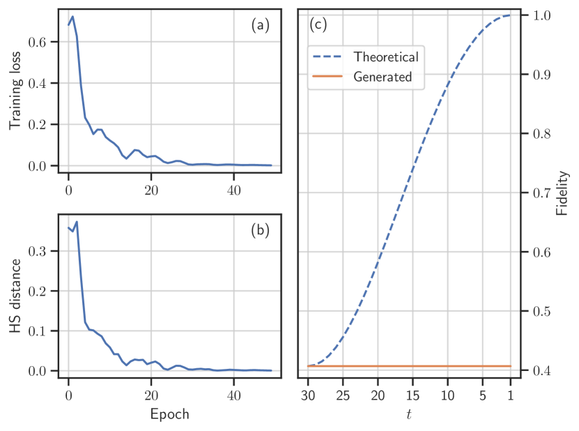
Figure 6: (a) Training loss with respect to the iterations of training. (b) Hilbert-Schmidt (HS) distance between the input and output state of denoising circuit $U(\boldsymbol{\theta})$. (c) After training, the generation fidelity of QGDM with respect to the timestep. The blue dashed line represents the theoretical fidelity that QGDM should achieve, showing the change in the generation process fidelity over timestep $t$. The orange solid line represents the actual generation fidelity.

The comparison between the final generated quantum state $\tilde{\rho}_{0}$ (shown in the first row) and the target quantum state $\rho_{0}$ (displayed in the second row) is illustrated in Fig. 7. Given the complex nature of each entries in a density matrix, the figure separately depicts the real and imaginary parts, with the former on the left and the latter on the right. This visualization clearly shows that $\tilde{\rho}_{0}$ closely resembles the completely mixed state $\rho_{T}$ , indicating that $U(\boldsymbol{\theta})$ essentially reproduces the input state. This highlights the critical need for a well-designed denoising process in QGDM that effectively integrates information between the noisy input state $\rho_{t}$ and the timestep embedding state $\tau_{t}$, especially considering the minor differences in quantum states across adjacent timesteps. The results and discussion in our study provide valuable insights for future development of similar quantum machine learning models.

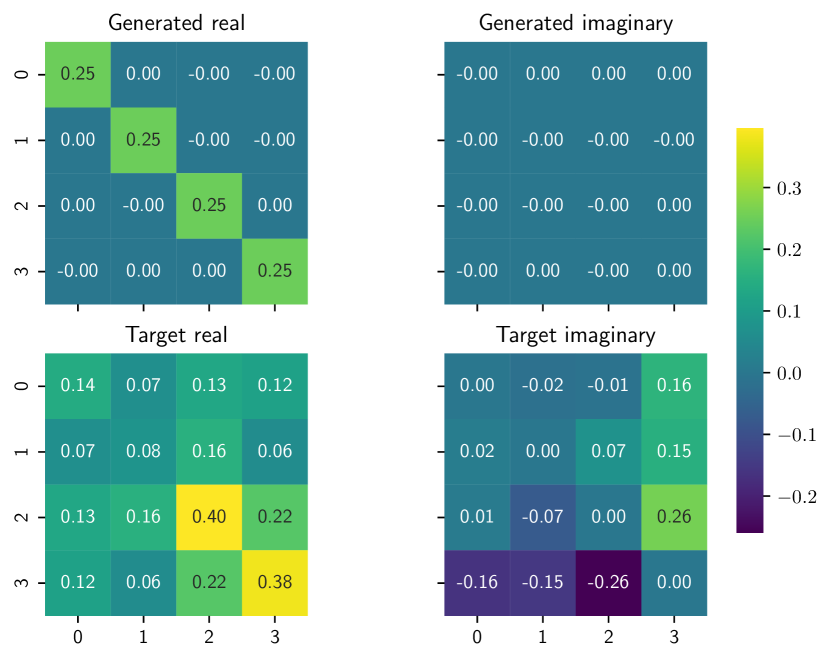
Figure 7: Visualization of the generated density matrix and target density matrix.

Finally, it is important to note that even though using the identity matrix $\mathbb{I}$ as a simple method to maintain the same input and output states for $U(\boldsymbol{\theta})$ seems straightforward, the learning algorithm does not always choose to do so. This is because different ensembles of quantum states, even when distinct at the microscopic level, can still be mapped to other ensembles with identical density matrices after transformation by $U(\boldsymbol{\theta})$. Essentially, these quantum state ensembles, despite their differences at the microscopic level, are capable of exhibiting similar statistical behaviors at the macroscopic scale. Consider the following simple example of a mixed state:

$$\sigma=0.5|0\rangle\langle 0|+0.5|1\rangle\langle 1|.$$ (15)

To ensure the input and output states of $U(\boldsymbol{\theta})$ remain identical, $i.e.$, satisfying the condition $U(\boldsymbol{\theta})\sigma U^{\dagger}(\boldsymbol{\theta})=\sigma$, we consider possible forms of $U(\boldsymbol{\theta})$. These could include the identity matrix $\mathbb{I}=\left[{\begin{array}[]{*{20}{c}}{\rm{1}}&{\rm{0}}\\ {\rm{0}}&{\rm{1}}\end{array}}\right]$ or the Hadamard matrix $H=\frac{1}{\sqrt{2}}\left[{\begin{array}[]{*{20}{c}}{\rm{1}}&{\rm{1}}\\ {\rm{1}}&{\rm{-1}}\end{array}}\right]$. The suitability of the Hadamard matrix, for instance, can be demonstrated as follows:

$$H\sigma H^{\dagger} =0.5|+\rangle\langle+|+0.5|-\rangle\langle-|$$ (16)

$$=0.5|0\rangle\langle 0|+0.5|1\rangle\langle 1|.$$

The learning algorithm does not necessarily adjust $U(\boldsymbol{\theta})$ to become the identity matrix $\mathbb{I}$, as various transformations within the hypothesis space can satisfy this condition. Which transformation is selected depends on where $U(\boldsymbol{\theta})$ is placed in the hypothesis space during parameter initialization.

VI Numerical Simulations

VI-A Setup

Our evaluation of the proposed models involved generating a variety of random quantum states, encompassing both pure and mixed states. We conducted a comparative analysis of our models against the QuGAN [13]. The implementation of the QuGAN is based on the original framework in Pennylane [73]. In our work, we use the Tensorcircuit framework [74] for simulating quantum circuits and the Tensorflow framework [75] for parameter optimization, with the optimizer Adam [76]. Due to our limited device resources, our numerical simulations covered qubits ranging from 1 to 8. QGDM results were achievable up to $N=4$, and RE-QGDM degenerates to QGDM at $N=1$. Therefore, in the next two subsection, results for QGBM at $N>4$ and RE-QGDM at $N=1$ are excluded. All simulations were repeated 10 times with different random seeds to ensure the robustness and reproducibility of our results.

VI-A1 Target Pure State Preparation

Fig. 8 illustrates our approach to obtaining a target quantum pure state $|\psi\rangle$. We utilize a combination of single-qubit gates and controlled $Rx$ blocks, as the $Rx$-$Rz$-$Rx$ gate combination can rotate the quantum state to any point on the surface of the Bloch Sphere. The controlled $Rx$ gates provide entanglement between the qubits. All parameters in the target state generation circuit are uniformly sampled from the range $[0,\pi]$.

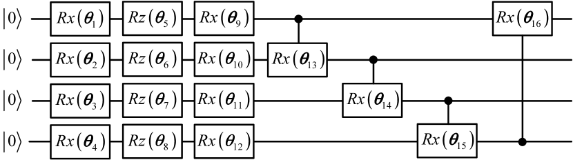
Figure 8: The architecture of a 4 qubits circuit to prepare a target pure state. All the parameters $\theta$ are initialize in $[0,\pi]$.

VI-A2 Target Mixed State Preparation

Quantum mixed states are generated through $\rho=\sum_{i}{p_{i}\left|\psi_{i}\right\rangle\left\langle\psi_{i}\right|}$, where $\{\left|\psi_{i}\right\rangle\}$ are randomly produced by the circuit shown in Fig. 8. The probability vector ${p_{i}}$ is obtained by uniform sampling from $(0,1]$ and normalized through a softmax operation to ensure $\sum_{i}{p_{i}}=1$ and $p_{i}>0$ for any index $i$.

VI-B Pure State Generation

We investigated the impact of $N_{\text{time}}$ on the generation of target pure states, with results shown in Fig. 9. This figure plots the fidelity of generated states against $N_{\text{time}}$ for systems with 1 to 4 qubits ($N$=1, 2, 3, 4), over a range of $N_{\text{time}}$ from 1 to $N+1$. In Fig. 9, generation fidelity improves with $N_{\text{time}}$ when $N_{\text{time}}\leq N$, achieving optimality at $N_{\text{time}}=N$ for all $N$.

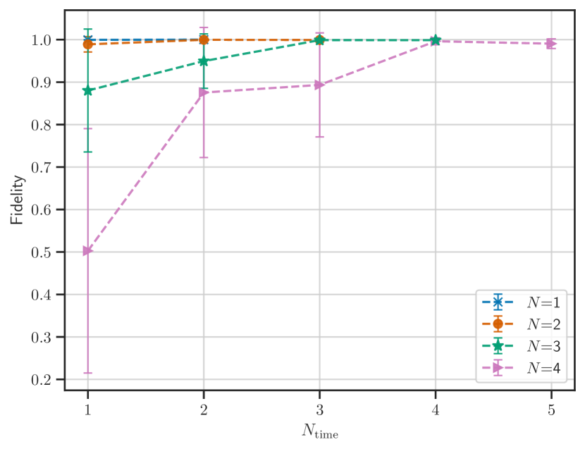
Figure 9: The generation fidelity of QGDM in generating target pure states for different qubits with respect to $N_{\text{time}}$. All data represent the average of 10 parallel experiments, and the error bars indicate the standard deviation.

However, when $N_{\text{time}}>N$, except for $N=1$, fidelity slightly decreases in other cases. The reason for this may be the following analysis. The circuit $U(\boldsymbol{\theta})$ operates on the combined system of $\tau_{t}$ and $\rho_{t}$, with the objective of merging their information and projecting the output onto the first $N$ qubits of the $\tau_{t}$ state system. It is worth noting that these first $N$ qubits of $\tau_{t}$ correspond to register A in Fig. 2. In cases when $N_{\text{time}}>N$, there is an extra qubit in the $\tau_{t}$ state system compared to $\rho_{t}$. This additional qubit from $\tau_{t}$, being redundant, complicates the process of merging and output prediction. Consequently, this leads to a slight decrease in model performance in scenarios when $N_{\text{time}}>N$.

When $N_{\text{time}}<N$, register A, which houses $\tau_{t}$, has an overlap of qubits from $\rho_{t}$. This overlap eases the integration task for $U(\theta)$ as part of the information from $\rho_{t}$ is already present in register A, potentially diminishing $U(\theta)$’s effectiveness in these instances. Section V explores a well-intentioned but flawed denoising design. This approach incorporates all qubits of $\rho_{t}$ into the output register, thus maximizing their overlap with the input qubits. Such results reinforce our previous observations, exemplifying the most extreme scenarios of this effect.

Based on the results in Fig. 9, subsequent simulations default to $N_{\text{time}}=N$ as this setting yields the best generative results with our proposed method.

TABLE II: Comparison of pure state generation between QuGAN and our proposed methods.

$N$	1	2	3	4	5	6	7	8
QuGAN[13]	0.999$\pm$5e-5	0.996$\pm$4e-3	0.995$\pm$4e-3	0.993$\pm$3e-3	0.990$\pm$4e-3	0.986$\pm$3e-3	0.978$\pm$6e-3	0.971$\pm$0.12
QGDM (Ours)	0.999$\pm$3e-5	0.999$\pm$2e-4	0.999$\pm$2e-3	0.996$\pm$8e-3	/	/	/	/
RE-QGDM (Ours)	/	0.994$\pm$8e-3	0.999$\pm$6e-4	0.999$\pm$4e-4	0.997$\pm$4e-3	0.995$\pm$0.011	0.994$\pm$4e-3	0.990$\pm$0.011

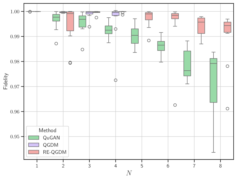
Figure 10: Pure state generation results.

In Fig. 10, we compared three quantum generative models: QuGAN[13], QGDM, and RE-QGDM, to assess their fidelity performance in generating target pure states with different qubit numbers. Using box plots to represent the distribution of results from 10 parallel experiments, the results indicate that the fidelity of all models decreases as the number of qubits in the target state increases. Specifically, the QuGAN model exhibits higher fidelity with lower qubit numbers, but as the number of qubits increases, its median fidelity rapidly decreases, and the variability in data distribution increases, indicating more outliers. At $N\geq 7$, all QuGAN data points fall below 0.99, suggesting potential limitations in handling more complex quantum states. Our two proposed methods (RE-) QGDM mostly maintain fidelity above 0.99 for all $N$, with relatively concentrated data distributions, demonstrating their stronger scalability. The QGDM model exhibits a moderate level of fidelity, performing better than the others at $N=1,2$. RE-QGDM’s median fidelity surpasses the other two models in most cases and shows greater stability with higher qubit numbers compared to QuGAN. In summary, QGDM demonstrates strong performance with smaller quantum systems, whereas RE-QGDM provides a more robust solution across a broader range of qubit configurations.

To more accurately assess the performance differences, we compare the pure state generation fidelity of QuGAN with our QGDM and RE-QGDM models at various qubit numbers, as detailed in Table II. QuGAN’s fidelity gradually declines with increasing $N$, from 0.999$\pm$5e-5 at $N=1$ to 0.971$\pm$0.12 at $N=8$. Notably, its fidelity falls below 0.99 for $N\geq 6$, indicating a decreasing trend in performance for larger quantum systems. QuGAN’s fidelity remains above 0.99 for $N=1$ to 5, though these values are consistently lower than those achieved by our proposed methods.

In comparison, QGDM maintains stable fidelity, averaging 0.999 at $N=1,2,3$, and sustaining a level of 0.996$\pm$8e-3 up to $N=4$. Significantly, the RE-QGDM model consistently exhibits high fidelity across all qubit numbers, reaching 0.99 even at $N=8$. This demonstrates RE-QGDM’s superior robustness in accurately generating states, underscoring the effectiveness and scalability of our approaches.

VI-C Mixed State Generation

Generating mixed states carries more substantial practical implications than pure states and presents increased challenges. Evaluating quantum generative models in the context of mixed state generation more effectively distinguishes their capabilities.

In Fig. 11, we assess the fidelity of three quantum generative models in generating mixed states. The findings show that while the QuGAN model experiences a fidelity decrease as the number of qubits ($N$) increases, both QGDM and RE-QGDM exhibit remarkable robustness, particularly at large-scale tasks. Specifically, QuGAN demonstrates a consistent drop in fidelity with increasing $N$, starting above 0.9 at $N=1$ but then falling sharply, with most fidelity scores and median values around 0.3. By contrast, QGDM outperforms QuGAN at $N=1$, with most results concentrated around 0.99. For $N=2,3$, and 4, RE-QGDM shows a slight edge over QGDM. Notably, at $N\geq 5$, RE-QGDM clearly surpasses QuGAN, maintaining all fidelity scores above 0.9.

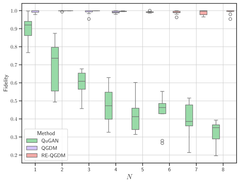
Figure 11: Mixed state generation results.

TABLE III: Comparison of mixed state generation performance between QuGAN and our proposed methods.

$N$	1	2	3	4	5	6	7	8
QuGAN[13]	0.902$\pm$0.066	0.694$\pm$0.134	0.598$\pm$0.069	0.477$\pm$0.092	0.414$\pm$0.084	0.439$\pm$0.092	0.396$\pm$0.089	0.324$\pm$0.062
QGDM (Ours)	0.995$\pm$7e-3	0.999$\pm$1e-3	0.992$\pm$0.013	0.992$\pm$7e-3	/	/	/	/
RE-QGDM (Ours)	/	0.999$\pm$6e-4	0.999$\pm$5e-4	0.996$\pm$2e-3	0.993$\pm$4e-3	0.990$\pm$0.011	0.992$\pm$0.018	0.993$\pm$0.015

In Table III, we present a detailed comparison of generation fidelity for mixed states among the three methods. QuGAN shows a fidelity of 0.902$\pm$0.066 starting from $N=1$, which declines to 0.324$\pm$0.062 at $N=8$. This trend reveals that QuGAN struggles with increasing $N$, highlighting its limited scalability in generating complex states. In contrast, QGDM and RE-QGDM consistently maintain a fidelity above 0.99 across all results, coupled with a low standard deviation. This consistency indicates that their performance is robust against random parameter variations. Notably, in some instances, our methods achieve a fidelity exceeding 0.999, showcasing their superior generative capabilities. Specifically, RE-QGDM reaches 0.992$\pm$0.018 at $N=7$ and maintains 0.993$\pm$0.015 at $N=8$, demonstrating our model’s ability to preserve high generation fidelity even with larger-scale problems. This consistent performance underscores our model’s aptitude for addressing complex, large-scale quantum generation tasks.

VII Conclusion

Drawing inspiration from classical diffusion models, this paper introduces the Quantum Generative Diffusion Models (QGDM), a novel quantum generative approach for producing quantum state ensembles. Similar to its classical counterparts, QGDM encompasses both a diffusion and a denoising process. In the diffusion phase, a timestep-dependent depolarizing channel incrementally converts the input state into a maximally random state, known as a completely mixed state. The denoising phase involves a parameterized function composed of a timestep embedding circuit and a denoising circuit, employing the concept of parameter sharing. Specifically, the timestep embedding circuit embeds temporal data into a quantum state, while the denoising circuit processes the noise-infused quantum state along with the timestep-embedded state to produce a denoised output, achieved by tracing out the noise component. To optimize QGDM’s resource efficiency, particularly regarding auxiliary qubit usage, we introduce the Resource-Efficient QGDM (RE-QGDM). Numerical simulations, conducted up to 8 qubits, compare our models with QuGAN. The results clearly indicate that both QGDM and RE-QGDM surpass QuGAN in generating both pure and mixed quantum states, highlighting their enhanced performance and scalability. Future endeavors will involve benchmarking (RE-) QGDM against other quantum generative models and delving deeper into the potential applications and capabilities of (RE-) QGDM.

References

- [1] S. Bond-Taylor, A. Leach, Y. Long, and C. G. Willcocks, “Deep generative modelling: A comparative review of vaes, gans, normalizing flows, energy-based and autoregressive models,” IEEE transactions on pattern analysis and machine intelligence, 2021.
- [2] Y. Cao, S. Li, Y. Liu, Z. Yan, Y. Dai, P. S. Yu, and L. Sun, “A comprehensive survey of ai-generated content (aigc): A history of generative ai from gan to chatgpt,” arxiv:2303.04226, 2023.
- [3] OpenAI, “Gpt-4 technical report,” https://cdn.openai.com/papers/gpt-4.pdf, 2023.
- [4] R. Rombach, A. Blattmann, D. Lorenz, P. Esser, and B. Ommer, “High-resolution image synthesis with latent diffusion models,” in Proceedings of the IEEE/CVF conference on computer vision and pattern recognition, 2022, pp. 10 684–10 695.
- [5] T. Wu, S. He, J. Liu, S. Sun, K. Liu, Q.-L. Han, and Y. Tang, “A brief overview of chatgpt: The history, status quo and potential future development,” IEEE/CAA Journal of Automatica Sinica, vol. 10, no. 5, pp. 1122–1136, 2023.
- [6] J. Tian, X. Sun, Y. Du, S. Zhao, Q. Liu, K. Zhang, W. Yi, W. Huang, C. Wang, X. Wu et al., “Recent advances for quantum neural networks in generative learning,” IEEE Transactions on Pattern Analysis and Machine Intelligence, 2023.
- [7] J. Biamonte, P. Wittek, N. Pancotti, P. Rebentrost, N. Wiebe, and S. Lloyd, “Quantum machine learning,” Nature, vol. 549, no. 7671, pp. 195–202, 2017.
- [8] M. Schuld and N. Killoran, “Quantum machine learning in feature hilbert spaces,” Physical review letters, vol. 122, no. 4, p. 040504, 2019.
- [9] M. Cerezo, A. Arrasmith, R. Babbush, S. C. Benjamin, S. Endo, K. Fujii, J. R. McClean, K. Mitarai, X. Yuan, L. Cincio et al., “Variational quantum algorithms,” Nature Reviews Physics, vol. 3, no. 9, pp. 625–644, 2021.
- [10] M. Cerezo, G. Verdon, H.-Y. Huang, L. Cincio, and P. J. Coles, “Challenges and opportunities in quantum machine learning,” Nature Computational Science, vol. 2, no. 9, pp. 567–576, 2022.
- [11] J. Shi, W. Wang, X. Lou, S. Zhang, and X. Li, “Parameterized hamiltonian learning with quantum circuit,” IEEE Transactions on Pattern Analysis and Machine Intelligence, vol. 45, no. 5, pp. 6086–6095, 2022.
- [12] S. Lloyd and C. Weedbrook, “Quantum generative adversarial learning,” Physical review letters, vol. 121, no. 4, p. 040502, 2018.
- [13] P.-L. Dallaire-Demers and N. Killoran, “Quantum generative adversarial networks,” Physical Review A, vol. 98, no. 1, p. 012324, 2018.
- [14] H. Situ, Z. He, Y. Wang, L. Li, and S. Zheng, “Quantum generative adversarial network for generating discrete distribution,” Information Sciences, vol. 538, pp. 193–208, 2020.
- [15] M. Benedetti, D. Garcia-Pintos, O. Perdomo, V. Leyton-Ortega, Y. Nam, and A. Perdomo-Ortiz, “A generative modeling approach for benchmarking and training shallow quantum circuits,” npj Quantum Information, vol. 5, no. 1, p. 45, 2019.
- [16] J.-G. Liu and L. Wang, “Differentiable learning of quantum circuit born machines,” Physical Review A, vol. 98, no. 6, p. 062324, 2018.
- [17] A. Khoshaman, W. Vinci, B. Denis, E. Andriyash, H. Sadeghi, and M. H. Amin, “Quantum variational autoencoder,” Quantum Science and Technology, vol. 4, no. 1, p. 014001, 2018.
- [18] M. H. Amin, E. Andriyash, J. Rolfe, B. Kulchytskyy, and R. Melko, “Quantum boltzmann machine,” Physical Review X, vol. 8, no. 2, p. 021050, 2018.
- [19] I. Goodfellow, J. Pouget-Abadie, M. Mirza, B. Xu, D. Warde-Farley, S. Ozair, A. Courville, and Y. Bengio, “Generative adversarial nets,” Advances in neural information processing systems, vol. 27, 2014.
- [20] S. Chakrabarti, H. Yiming, T. Li, S. Feizi, and X. Wu, “Quantum wasserstein generative adversarial networks,” Advances in Neural Information Processing Systems, vol. 32, 2019.
- [21] M. Y. Niu, A. Zlokapa, M. Broughton, S. Boixo, M. Mohseni, V. Smelyanskyi, and H. Neven, “Entangling quantum generative adversarial networks,” Physical Review Letters, vol. 128, no. 22, p. 220505, 2022.
- [22] H.-L. Huang, Y. Du, M. Gong, Y. Zhao, Y. Wu, C. Wang, S. Li, F. Liang, J. Lin, Y. Xu et al., “Experimental quantum generative adversarial networks for image generation,” Physical Review Applied, vol. 16, no. 2, p. 024051, 2021.
- [23] D. Silver, T. Patel, W. Cutler, A. Ranjan, H. Gandhi, and D. Tiwari, “Mosaiq: Quantum generative adversarial networks for image generation on nisq computers,” in Proceedings of the IEEE/CVF International Conference on Computer Vision, 2023, pp. 7030–7039.
- [24] S. L. Tsang, M. T. West, S. M. Erfani, and M. Usman, “Hybrid quantum-classical generative adversarial network for high resolution image generation,” IEEE Transactions on Quantum Engineering, 2023.
- [25] J. Zeng, Y. Wu, J.-G. Liu, L. Wang, and J. Hu, “Learning and inference on generative adversarial quantum circuits,” Physical Review A, vol. 99, no. 5, p. 052306, 2019.
- [26] S. Chaudhary, P. Huembeli, I. MacCormack, T. L. Patti, J. Kossaifi, and A. Galda, “Towards a scalable discrete quantum generative adversarial neural network,” Quantum Science and Technology, vol. 8, no. 3, p. 035002, 2023.
- [27] P. Braccia, F. Caruso, and L. Banchi, “How to enhance quantum generative adversarial learning of noisy information,” New Journal of Physics, vol. 23, no. 5, p. 053024, 2021.
- [28] J. Sohl-Dickstein, E. Weiss, N. Maheswaranathan, and S. Ganguli, “Deep unsupervised learning using nonequilibrium thermodynamics,” in International conference on machine learning. PMLR, 2015, pp. 2256–2265.
- [29] J. Ho, A. Jain, and P. Abbeel, “Denoising diffusion probabilistic models,” Advances in neural information processing systems, vol. 33, pp. 6840–6851, 2020.
- [30] J. Song, C. Meng, and S. Ermon, “Denoising diffusion implicit models,” in International Conference on Learning Representations, 2020.
- [31] A. Q. Nichol and P. Dhariwal, “Improved denoising diffusion probabilistic models,” in International Conference on Machine Learning. PMLR, 2021, pp. 8162–8171.
- [32] P. Dhariwal and A. Nichol, “Diffusion models beat gans on image synthesis,” Advances in neural information processing systems, vol. 34, pp. 8780–8794, 2021.
- [33] C. Luo, “Understanding diffusion models: A unified perspective,” arxiv:2208.11970, 2022.
- [34] Y. Du, M.-H. Hsieh, T. Liu, and D. Tao, “Expressive power of parametrized quantum circuits,” Physical Review Research, vol. 2, no. 3, p. 033125, 2020.
- [35] D. Zhu, N. M. Linke, M. Benedetti, K. A. Landsman, N. H. Nguyen, C. H. Alderete, A. Perdomo-Ortiz, N. Korda, A. Garfoot, C. Brecque et al., “Training of quantum circuits on a hybrid quantum computer,” Science advances, vol. 5, no. 10, p. eaaw9918, 2019.
- [36] B. Coyle, D. Mills, V. Danos, and E. Kashefi, “The born supremacy: quantum advantage and training of an ising born machine,” npj Quantum Information, vol. 6, no. 1, p. 60, 2020.
- [37] O. Kiss, M. Grossi, E. Kajomovitz, and S. Vallecorsa, “Conditional born machine for monte carlo event generation,” Physical Review A, vol. 106, no. 2, p. 022612, 2022.
- [38] B. Coyle, M. Henderson, J. C. J. Le, N. Kumar, M. Paini, and E. Kashefi, “Quantum versus classical generative modelling in finance,” Quantum Science and Technology, vol. 6, no. 2, p. 024013, 2021.
- [39] J. Alcazar, V. Leyton-Ortega, and A. Perdomo-Ortiz, “Classical versus quantum models in machine learning: insights from a finance application,” Machine Learning: Science and Technology, vol. 1, no. 3, p. 035003, 2020.
- [40] E. Y. Zhu, S. Johri, D. Bacon, M. Esencan, J. Kim, M. Muir, N. Murgai, J. Nguyen, N. Pisenti, A. Schouela et al., “Generative quantum learning of joint probability distribution functions,” Physical Review Research, vol. 4, no. 4, p. 043092, 2022.
- [41] S. E. Fahlman, G. E. Hinton, and T. J. Sejnowski, “Massively parallel architectures for al: Netl, thistle, and boltzmann machines,” in National Conference on Artificial Intelligence, AAAI, 1983.
- [42] D. H. Ackley, G. E. Hinton, and T. J. Sejnowski, “A learning algorithm for boltzmann machines,” Cognitive science, vol. 9, no. 1, pp. 147–169, 1985.
- [43] M. Kieferová and N. Wiebe, “Tomography and generative training with quantum boltzmann machines,” Physical Review A, vol. 96, no. 6, p. 062327, 2017.
- [44] D. Crawford, A. Levit, N. Ghadermarzy, J. S. Oberoi, and P. Ronagh, “Reinforcement learning using quantum boltzmann machines,” arxiv:1612.05695, 2016.
- [45] C. Zoufal, A. Lucchi, and S. Woerner, “Variational quantum boltzmann machines,” Quantum Machine Intelligence, vol. 3, pp. 1–15, 2021.
- [46] J. T. Rolfe, “Discrete variational autoencoders,” arxiv:1609.02200, 2016.
- [47] N. Gao, M. Wilson, T. Vandal, W. Vinci, R. Nemani, and E. Rieffel, “High-dimensional similarity search with quantum-assisted variational autoencoder,” in Proceedings of the 26th ACM SIGKDD international conference on knowledge discovery & data mining, 2020, pp. 956–964.
- [48] J. Li and S. Ghosh, “Scalable variational quantum circuits for autoencoder-based drug discovery,” in 2022 Design, Automation & Test in Europe Conference & Exhibition (DATE). IEEE, 2022, pp. 340–345.
- [49] M. Benedetti, E. Grant, L. Wossnig, and S. Severini, “Adversarial quantum circuit learning for pure state approximation,” New Journal of Physics, vol. 21, no. 4, p. 043023, 2019.
- [50] M. Parigi, S. Martina, and F. Caruso, “Quantum-noise-driven generative diffusion models,” arxiv:2308.12013, 2023.
- [51] B. Zhang, P. Xu, X. Chen, and Q. Zhuang, “Generative quantum machine learning via denoising diffusion probabilistic models,” arxiv:2310.05866, 2023.
- [52] A. Cacioppo, L. Colantonio, S. Bordoni, and S. Giagu, “Quantum diffusion models,” arxiv:2311.15444, 2023.
- [53] W. H. Zurek, “Decoherence, einselection, and the quantum origins of the classical,” Reviews of modern physics, vol. 75, no. 3, p. 715, 2003.
- [54] R. Horodecki, P. Horodecki, M. Horodecki, and K. Horodecki, “Quantum entanglement,” Reviews of modern physics, vol. 81, no. 2, p. 865, 2009.
- [55] A. Streltsov, G. Adesso, and M. B. Plenio, “Colloquium: Quantum coherence as a resource,” Reviews of Modern Physics, vol. 89, no. 4, p. 041003, 2017.
- [56] I. M. Georgescu, S. Ashhab, and F. Nori, “Quantum simulation,” Reviews of Modern Physics, vol. 86, no. 1, p. 153, 2014.
- [57] M. A. Nielsen and I. L. Chuang, Quantum computation and quantum information. Cambridge university press, 2010.
- [58] S. R. De Groot and P. Mazur, Non-equilibrium thermodynamics. Courier Corporation, 2013.
- [59] M. M. Wilde, Quantum information theory. Cambridge university press, 2013.
- [60] D. P. Kingma and M. Welling, “Auto-encoding variational bayes,” arxiv:1312.6114, 2013.
- [61] D. Kingma, T. Salimans, B. Poole, and J. Ho, “Variational diffusion models,” Advances in neural information processing systems, vol. 34, pp. 21 696–21 707, 2021.
- [62] E. Stoudenmire and D. J. Schwab, “Supervised learning with tensor networks,” Advances in neural information processing systems, vol. 29, 2016.
- [63] E. Grant, M. Benedetti, S. Cao, A. Hallam, J. Lockhart, V. Stojevic, A. G. Green, and S. Severini, “Hierarchical quantum classifiers,” npj Quantum Information, vol. 4, no. 1, p. 65, 2018.
- [64] M. Schuld and F. Petruccione, Supervised learning with quantum computers. Springer, 2018, vol. 17.
- [65] P. Rebentrost, M. Mohseni, and S. Lloyd, “Quantum support vector machine for big data classification,” Physical review letters, vol. 113, no. 13, p. 130503, 2014.
- [66] Z. He, L. Li, S. Zheng, Y. Li, and H. Situ, “Variational quantum compiling with double q-learning,” New Journal of Physics, vol. 23, no. 3, p. 033002, 2021.
- [67] M. Ostaszewski, L. M. Trenkwalder, W. Masarczyk, E. Scerri, and V. Dunjko, “Reinforcement learning for optimization of variational quantum circuit architectures,” Advances in Neural Information Processing Systems, vol. 34, pp. 18 182–18 194, 2021.
- [68] S.-X. Zhang, C.-Y. Hsieh, S. Zhang, and H. Yao, “Differentiable quantum architecture search,” Quantum Science and Technology, vol. 7, no. 4, p. 045023, 2022.
- [69] Y. Du, T. Huang, S. You, M.-H. Hsieh, and D. Tao, “Quantum circuit architecture search for variational quantum algorithms,” npj Quantum Information, vol. 8, no. 1, p. 62, 2022.
- [70] Z. He, C. Chen, L. Li, S. Zheng, and H. Situ, “Quantum architecture search with meta-learning,” Advanced Quantum Technologies, vol. 5, no. 8, p. 2100134, 2022.
- [71] Z. He, M. Deng, S. Zheng, L. Li, and H. Situ, “Gsqas: Graph self-supervised quantum architecture search,” Physica A: Statistical Mechanics and its Applications, vol. 630, p. 129286, 2023.
- [72] Z. He, X. Zhang, C. Chen, Z. Huang, Y. Zhou, and H. Situ, “A gnn-based predictor for quantum architecture search,” Quantum Information Processing, vol. 22, no. 2, p. 128, 2023.
- [73] V. Bergholm, J. Izaac, M. Schuld, C. Gogolin, S. Ahmed, V. Ajith, M. S. Alam, G. Alonso-Linaje, B. AkashNarayanan, A. Asadi et al., “Pennylane: Automatic differentiation of hybrid quantum-classical computations,” arxiv:1811.04968, 2018.
- [74] S.-X. Zhang, J. Allcock, Z.-Q. Wan, S. Liu, J. Sun, H. Yu, X.-H. Yang, J. Qiu, Z. Ye, Y.-Q. Chen et al., “Tensorcircuit: a quantum software framework for the nisq era,” Quantum, vol. 7, p. 912, 2023.
- [75] M. Abadi, A. Agarwal, P. Barham, E. Brevdo, Z. Chen, C. Citro, G. S. Corrado, A. Davis, J. Dean, M. Devin, S. Ghemawat, I. Goodfellow, A. Harp, G. Irving, M. Isard, Y. Jia, R. Jozefowicz, L. Kaiser, M. Kudlur, J. Levenberg, D. Mané, R. Monga, S. Moore, D. Murray, C. Olah, M. Schuster, J. Shlens, B. Steiner, I. Sutskever, K. Talwar, P. Tucker, V. Vanhoucke, V. Vasudevan, F. Viégas, O. Vinyals, P. Warden, M. Wattenberg, M. Wicke, Y. Yu, and X. Zheng, “TensorFlow: Large-scale machine learning on heterogeneous systems,” 2015, software available from tensorflow.org. [Online]. Available: https://www.tensorflow.org/
- [76] D. P. Kingma and J. Ba, “Adam: A method for stochastic optimization,” arxiv:1412.6980, 2014.