A simple stochastic nonlinear AR model with application to bubble

Abstract

Economic and financial time series can feature locally explosive behavior when a bubble is formed. The economic or financial bubble, especially its dynamics, is an intriguing topic that has been attracting longstanding attention. To illustrate the dynamics of the local explosion itself, the paper presents a novel, simple, yet useful time series model, called the stochastic nonlinear autoregressive model, which is always strictly stationary and geometrically ergodic and can create long swings or persistence observed in many macroeconomic variables. When a nonlinear autoregressive coefficient is outside of a certain range, the model has periodically explosive behaviors and can then be used to portray the bubble dynamics. Further, the quasi-maximum likelihood estimation (QMLE) of our model is considered, and its strong consistency and asymptotic normality are established under minimal assumptions on innovation. A new model diagnostic checking statistic is developed for model fitting adequacy. In addition two methods for bubble tagging are proposed, one from the residual perspective and the other from the null-state perspective. Monte Carlo simulation studies are conducted to assess the performances of the QMLE and the two bubble tagging methods in finite samples. Finally, the usefulness of the model is illustrated by an empirical application to the monthly Hang Seng Index.

Keywords: Causal process, QMLE, Rational expectation, SNAR model, Speculative bubble.

1 Introduction

Financial speculative bubbles have been attracting longstanding attention of economists and financial practitioners as an economic crisis often originates along with a burst of a bubble. In reality, however, economic or financial bubbles cannot be avoided. The presence of bubbles is partially evidenced by that many economic or financial time series possess locally explosive behavior and a subsequent burst, with such a phenomenon appearing periodically. Studying the dynamics of bubble thus becomes important and intriguing.

One classical definition of the bubble is the deviation of the market price from its fundamental value (a sum of discounted future dividends) in rational expectation price models. An important model of the rational bubble is initiated by Blanchard and Watson (1982), where the bubble process is captured via a simple stochastic autoregression (AR) with a fixed explosive rate and an absorbing state zero. Their model is then extended by Evans (1991) via adopting a stochastic rate of explosion. Primarily, the bubble is regarded as an explosive nonstationary process, which motivates to test its presence via unit root and cointegration tests (Diba and Grossman, 1988a, b). Recently, this idea is further developed by Phillips and Yu (2011), Phillips et al. (2011, 2015a, 2015b), Harvey et al. (2019, 2020), Tao et al. (2019), Kurozumi et al. (2022), Esteve and Prats (2023) and references therein. On the other hand, Evans (1991) also notes that periodical collapse of bubbles makes the bubble paths look more like a stationary process. Within a stationary framework, Gouriéroux and Zakoïan (2017) find that noncausal AR(1) models can characterize multiple local explosions in time series. Then this noncausal approach to bubble modelling has been extended to high-order mixed causal-noncausal time series models, see, for example, Gouriéroux and Jasiak (2016), Fries and Zakoïan (2019), Cavaliere et al. (2020), Davis and Song (2020), and Fries (2022). However, one shortcoming of the noncausal approach invites computational challenge and many resampling methods are needed. To bypass this shortcoming, Blasques et al. (2022) propose a new observation driven model with time-varying parameters and study its probabilistic properties and statistical inference. Nevertheless, their estimation heavily depends on the choice of the survival function and the asymptotics can be obtained only for a part of parameters. Motivated by all above facts, we here present a new simple time series model to describe the dynamics of bubbles.

In this paper, a first-order stochastic nonlinear autoregressive (SNAR) model $\{y_{t}\}$ is defined as

$$y_{t}=s_{t}\phi_{0}|y_{t-1}|+\varepsilon_{t},\quad t\in\mathbb{Z}:=\{0,\pm 1,\pm 2,...\},$$ (1)

where $\phi_{0}\in\mathbb{R}$, $\{\varepsilon_{t}:\,t\in\mathbb{Z}\}$ is a sequence of independent and identically distributed (i.i.d.) random variables on some basic probability space $(\Omega,\mathcal{F},\mathbb{P})$, and independent of i.i.d. binary variables $\{s_{t}:\,t\in\mathbb{Z}\}$ with $\mathbb{P}(s_{t}=1)=p_{0}=1-\mathbb{P}(s_{t}=0)$, $p_{0}\in[0,1)$.

Clearly, when $\phi_{0}>1$, $y_{t}$ is explosive in the periods where $s_{t}=1$ and creates an excursion which stops once $s_{t}=0$. Fig. 1 illustrates two simulated paths of the SNAR model (1) with $\varepsilon_{t}\stackrel{{\scriptstyle i.i.d}}{{\sim}}\mathcal{N}(0,6^{2})$. We can observe periodically local explosions followed by bursts. Further, when $\mathbb{P}(s_{t}=1)=1$, the SNAR model (1) reduces to an absolute AR model or a special threshold AR model with threshold parameter zero, which is studied in Tong (1990), Li and Tong (2020) and references therein.

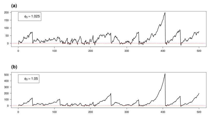
Figure 1: Simulated paths of model (1) with $\varepsilon_{t}\sim\mathcal{N}(0,6^{2})$, $p_{0}=0.977$, and (a) $\phi_{0}=1.025$ and (b) $\phi_{0}=1.05$.

Major contributions of our paper are as follows.

First, we introduce a simple yet useful time series model, a SNAR model, for modeling the dynamics of bubble process. We then prove that the model is always strictly stationary and geometrically ergodic under minimal assumptions on innovation and the probability $p_{0}$. Within a causal and stationary framework, when the parameter $\phi_{0}>1$, our SNAR model still displays periodically local explosions and collapses. It can create long swings or persistence and can then be used to portray the bubble dynamics. More importantly, our model is always causal in the classical sense of time series. Compared with the noncausal bubble models in the literature, our model facilitates the understanding of the dynamics of bubble, and is quite simpler and more convenient in application. Additionally, our model avoids computational burden of the noncausal approach and keeps away from the choice of the survival function in the time-varying parameter model in Blasques et al. (2022).

It is worth mentioning that a related model to ours is a stochastic AR initiated by Blanchard and Watson (1982), which is defined as $y_{t}=s_{t}\phi_{0}y_{t-1}+\varepsilon_{t}$, $t\in\mathbb{Z}$, where $\{s_{t}\}$ and $\{\varepsilon_{t}\}$ are defined in (1). It can also create long swings or persistence (Johansen and Lange, 2013). Unfortunately, it can usually generate many negative local explosions even if $\phi_{0}>1$ and $\varepsilon_{t}\stackrel{{\scriptstyle i.i.d}}{{\sim}}\mathcal{N}(0,1)$. This does not meet our common sense on financial bubble.

Second, we consider the quasi-maximum likelihood estimation (QMLE) of the SNAR model and establish its strong consistency and asymptotic normality under minimal assumptions on innovation and probability parameter $p_{0}$, regardless of infinite variance or heavy-tailedness of the model.

Third, we develop a new model diagnostic checking statistic since the classical portmanteau test is invalid for our model.

Fourth, we consider two methods for tagging the bubbles, one from the residual point of view and the other from the null-state perspective. The problem of bubble detection has been studied in the literature; see for example Phillips and Yu (2011), Phillips et al. (2015a), Phillips et al. (2015b), Blasques et al. (2022), Kurozumi and Skrobotov (2023), and references therein. Existing results in this direction, however, have been mainly developed by viewing the bubble as a separate process occurring on an unknown but deterministic time interval within the observation period. The current paper, on the other hand, aims to incorporate the bubble mechanism into the data generating process to provide a stationary statistical model that can capture and interpret bubbles, including their formations and collapses. As a result, unlike existing results that typically assume the bubbles to persist for an adequate duration to achieve their consistent detection, the bubbles in the current model can be transient and thus the problem of bubble tagging can be more challenging in the current setting. For this, we consider two approaches, where the first one utilizes the nonlinear autoregressive residual from the proposed model and the second one is constructed from a hypothesis testing point of view. For both methods, we provide theoretical quantification on the finite-sample probability of correct tagging under reasonably mild conditions. Monte Carlo simulation results are provided to assess the finite-sample performance of the proposed QMLE and bubble tagging methods.

The remainder of the paper is organized as follows. Section 2 investigates strict stationarity and geometric ergodicity of model (1). Section 3 considers the QMLE with its asymptotics. Section 4 studies model diagnostic checking. Section 5 considers the problem of bubble tagging, where two approaches are considered with their finite-sample probability bounds studied. Section 6 carries out Monte Carlo simulation studies to assess the finite-sample performances of the QMLE and the two bubble tagging methods. Section 7 gives an empirical application to illustrate the usefulness of the model. Section 8 concludes. All technical proofs are relegated to the Supplementary Material.

2 Probabilistic Properties of the SNAR Model

The aim of this section is to prove the strict stationarity and geometric ergodicity of model (1) under a very mild condition. We will prove the following result, using the approach developed by Meyn and Tweedie (2009) for establishing the geometric ergodicity of Markov chains. This result is important and is a theoretical foundation of statistical inference for model (1).

Theorem 1

Suppose that $\mathrm{(i)}$ $\{\varepsilon_{t}\}$ is i.i.d. and independent of i.i.d. binary variables $\{s_{t}\}$ with $0\leq p_{0}<1$, and $\mathrm{(ii)}$ $\varepsilon_{1}$ has a positive density on $\mathbb{R}$ with $\mathbb{E}(\log^{+}|\varepsilon_{1}|)<\infty$. Then there exists a strictly stationary, nonanticipative solution to $\{y_{t}\}$ in model $(\ref{eq.model})$ and the solution is unique and geometrically ergodic.

Next, consider the existence conditions on moments of $y_{t}$. Clearly, when $\mathbb{E}\varepsilon_{t}=0$, $\mathbb{E}\varepsilon_{t}^{2}<\infty$, and both $\varepsilon_{t}$ and $s_{t}$ are independent, then $\mathbb{E}y_{t}^{2}=\mathbb{E}\varepsilon_{t}^{2}/(1-p_{0}\phi_{0}^{2})<\infty$ if $p_{0}\phi_{0}^{2}<1$. Fig. 2 plots the strict stationarity region of $y_{t}$ with $\mathbb{E}y_{t}^{2}<\infty$.

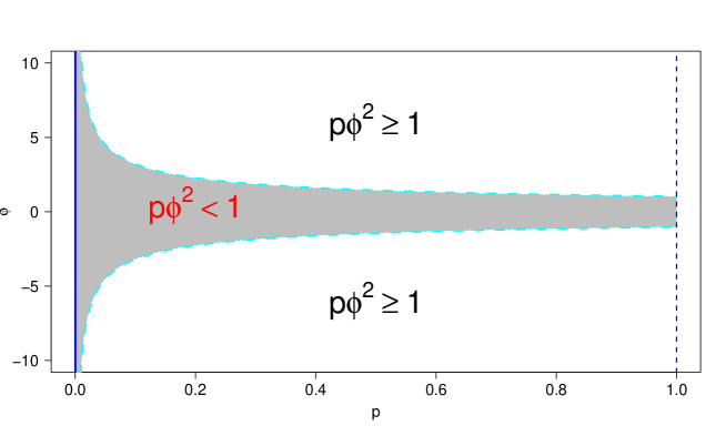
Figure 2: The strict stationarity region $\{(p,\phi):\,\phi\in\mathbb{R},\,p\phi^{2}<1,\,0\leq p<1\}$ of $y_{t}$ with finite second moment.

Further, if $\mathbb{E}\varepsilon_{t}^{3}=0$, then a simple algebraic calculation gives the kurtosis of $y_{t}$:

$$\mathrm{kurtosis}(y_{t})=\frac{\left\{6p_{0}\phi_{0}^{2}+\mathrm{kurtosis(\varepsilon_{t})}(1-p_{0}\phi_{0}^{2})\right\}(1-p_{0}\phi_{0}^{2})}{1-p_{0}\phi_{0}^{4}},\quad\mbox{if}\quad p_{0}\phi_{0}^{4}<1.$$

In particular, when $\varepsilon_{t}\sim\mathcal{N}(0,1)$, then

$$\mathrm{kurtosis}(y_{t})=\frac{3(1-p_{0}^{2}\phi_{0}^{4})}{1-p_{0}\phi_{0}^{4}}>3,\quad\mbox{if}\quad 0<p_{0}\phi_{0}^{4}<1,$$

which implies that $\{y_{t}\}$ must be heavy-tailed.

3 Quasi-Maximum Likelihood Estimation

Let $\theta_{0}=(\phi_{0},p_{0},\sigma_{0}^{2})^{\prime}$ be the true parameter with $\sigma^{2}_{0}=\mathbb{E}\varepsilon_{t}^{2}$. Denote by $\theta=(\phi,p,\sigma^{2})^{\prime}$ be the parameter and by $\Theta$ be the parameter space. Assume that the observations $\{y_{0},y_{1},...,y_{n}\}$ are from model (1) with the true value $\theta_{0}$. Clearly, under Assumption 1 below, it follows that $\mathbb{E}(y_{t}|y_{t-1})=p\phi|y_{t-1}|$ and $\mathrm{Var}(y_{t}|y_{t-1})=p(1-p)\phi^{2}y_{t-1}^{2}+\sigma^{2}$. Then the (conditional) log-quasi-likelihood function (omitting a constant) is

$$L_{n}(\theta)=\sum_{t=1}^{n}\ell_{t}(\theta):=\sum_{t=1}^{n}\left\{\log\left[p(1-p)\phi^{2}y_{t-1}^{2}+\sigma^{2}\right]+\frac{(y_{t}-p\phi|y_{t-1}|)^{2}}{p(1-p)\phi^{2}y_{t-1}^{2}+\sigma^{2}}\right\}.$$

The QMLE of $\theta_{0}$ is defined as

$$\widehat{\theta}_{n}=\arg\min_{\theta\in\Theta}L_{n}(\theta).$$

To study the asymptotics of $\widehat{\theta}_{n}$, the following two assumptions are needed.

Assumption 1

$\{\varepsilon_{t}\}$ is i.i.d. and independent of i.i.d. binary variables $\{s_{t}\}$ with $p_{0}<1$. Further, $\varepsilon_{1}$ has a positive density on $\mathbb{R}$ with zero mean and finite variance.

Assumption 2

The parameter space $\Theta$ is a compact subset of $\{\theta=(\phi,p,\sigma^{2})^{\prime}:\phi\neq 0,\,0<p<1,\,0<\sigma^{2}<\infty\}$.

The following theorems states the strong consistency and the asymptotic normality of $\widehat{\theta}_{n}$.

Theorem 2

If Assumptions 1-2 hold, then $\widehat{\theta}_{n}\rightarrow\theta_{0}$ a.s. as $n\rightarrow\infty$.

Theorem 3

If Assumptions 1-2 hold, $\mathbb{E}(\varepsilon_{t}^{4})<\infty$, and $\theta_{0}$ is an interior point of $\Theta$, then

$$\sqrt{n}\big{(}\widehat{\theta}_{n}-\theta_{0}\big{)}\stackrel{{\scriptstyle d}}{{\longrightarrow}}\mathcal{N}\left(0,\,\mathcal{J}^{-1}\mathcal{I}\mathcal{J}^{-1}\right),\quad\mbox{as $n\to\infty$},$$

where ‘$\stackrel{{\scriptstyle d}}{{\longrightarrow}}$’ stands for convergence in distribution,

$$\mathcal{J}=\mathbb{E}\left\{\frac{1}{[p_{0}(1-p_{0})\phi^{2}_{0}y_{t}^{2}+\sigma^{2}_{0}]^{2}}\mathbf{A}_{t}\right\}+\mathbb{E}\left\{\frac{2y_{t}^{2}}{p_{0}(1-p_{0})\phi^{2}_{0}y_{t}^{2}+\sigma^{2}_{0}}\right\}\mathbf{D},$$

$$\mathcal{I} =\mathbb{E}\left\{\frac{p_{0}(1-p_{0})(1-2p_{0})^{2}\phi^{4}_{0}y_{t}^{4}+4\sigma_{0}^{2}p_{0}(1-p_{0})\phi_{0}^{2}y_{t}^{2}+(\kappa_{4}-\sigma^{4}_{0})}{[p_{0}(1-p_{0})\phi^{2}_{0}y_{t}^{2}+\sigma^{2}_{0}]^{4}}\mathbf{A}_{t}\right\}$$

$$\quad+\mathbb{E}\left\{\frac{4y^{2}_{t}}{p_{0}(1-p_{0})\phi^{2}_{0}y_{t}^{2}+\sigma^{2}_{0}}\right\}\mathbf{D}+\mathbb{E}\left\{\frac{2p_{0}(1-p_{0})(1-2p_{0})\phi_{0}^{3}y_{t}^{4}+2|y_{t}|\kappa_{3}}{[p_{0}(1-p_{0})\phi^{2}_{0}y_{t}^{2}+\sigma^{2}_{0}]^{3}}\mathbf{B}_{t}\right\}$$

with $\kappa_{3}=\mathbb{E}(\varepsilon_{t}^{3})$, $\kappa_{4}=\mathbb{E}(\varepsilon_{t}^{4})$, and

$$\mathbf{A}_{t} =\left(\begin{array}[]{ccc}4p^{2}_{0}(1-p_{0})^{2}\phi^{2}_{0}y_{t}^{4}&2p_{0}(1-p_{0})(1-2p_{0})\phi^{3}_{0}y_{t}^{4}&2p_{0}(1-p_{0})\phi_{0}y_{t}^{2}\\ &(1-2p_{0})^{2}\phi^{4}_{0}y_{t}^{4}&(1-2p_{0})\phi^{2}_{0}y_{t}^{2}\\ &&1\end{array}\right),$$

$$\mathbf{B}_{t} =\left(\begin{array}[]{ccc}4p_{0}^{2}(1-p_{0})\phi_{0}y_{t}^{2}&p_{0}(3-4p_{0})\phi^{2}_{0}y_{t}^{2}&p_{0}\\ &2(1-2p_{0})\phi^{3}_{0}y_{t}^{2}&\phi_{0}\\ &&0\end{array}\right),\quad\mbox{and}\quad\mathbf{D}=\left(\begin{array}[]{ccc}p^{2}_{0}&p_{0}\phi_{0}&0\\ &\phi^{2}_{0}&0\\ &&0\end{array}\right).$$

Here, the elements in the lower triangles can be completed by symmetry.

Remark 1. From the expressions of the matrices $\mathcal{I}$ and $\mathcal{J}$ in Theorem 3, we can see that each element of random matrices within the expectation is bounded and thus it is unnecessary to require moment conditions on $y_{t}$ for the asymptotics of $\widehat{\theta}_{n}$.

Remark 2. In practice, to make statistical inference on $\theta_{0}$, we must estimate the matrices $\mathcal{I}$ and $\mathcal{J}$. From the proof of Theorem 3, they can be consistently estimated by

$$\widehat{\mathcal{I}}_{n}=\frac{1}{n}\sum_{t=1}^{n}\frac{\partial\ell_{t}(\widehat{\theta}_{n})}{\partial\theta}\frac{\partial\ell_{t}(\widehat{\theta}_{n})}{\partial\theta^{\prime}}\quad\mbox{and}\quad\widehat{\mathcal{J}}_{n}=\frac{1}{n}\sum_{t=1}^{n}\frac{\partial^{2}\ell_{t}(\widehat{\theta}_{n})}{\partial\theta\partial\theta^{\prime}},$$

respectively. Note that the plug-in method is here invalid since both $\kappa_{3}$ and $\kappa_{4}$ in $\mathcal{I}$ cannot be estimated from the residuals. Additionally, due to the constraint $p_{0}\in(0,1)$, the Delta method may be needed to construct confidence intervals of $p_{0}$. If necessary, for example, we can consider the transformation $g(p)=\log[(1-p)/p]$ for $p\in(0,1)$. Note that

$$\sqrt{n}\big{(}g(\widehat{p}_{n})-g(p_{0})\big{)}\stackrel{{\scriptstyle d}}{{\longrightarrow}}\frac{\lambda_{p}}{p_{0}(1-p_{0})}\mathcal{N}(0,1),$$

if $\sqrt{n}(\widehat{p}_{n}-p_{0})\stackrel{{\scriptstyle d}}{{\longrightarrow}}\mathcal{N}(0,\lambda_{p}^{2})$. Then, for any fixed $\alpha\in(0,1)$, a $100(1-\alpha)\%$ confidence interval of $p_{0}$ is

$$\left[\Big{\{}1+\exp\Big{[}g(\widehat{p}_{n})-\frac{\lambda_{p}\,z_{\alpha/2}}{\sqrt{n}\widehat{p}_{n}(1-\widehat{p}_{n})}\Big{]}\Big{\}}^{-1},\,\>\Big{\{}1+\exp\Big{[}g(\widehat{p}_{n})+\frac{\lambda_{p}\,z_{\alpha/2}}{\sqrt{n}\widehat{p}_{n}(1-\widehat{p}_{n})}\Big{]}\Big{\}}^{-1}\right],$$

where $z_{\alpha/2}$ is the lower $\alpha/2$-quantile of the standard normal.

4 Model Diagnostic Checking

Diagnostic checking is important for time series modeling. The most commonly used tool is the portmanteau test, which depends on the autocorrelation of the residuals or the squared residuals, see, e.g., McLeod and Li (1983), Li and Mak (1994), Li (2004), and Chen and Zhu (2015). However, such the portmanteau test fails for the adequacy of model (1) since the residuals cannot be obtained. In fact, the residuals should be theoretically calculated by $\widehat{\varepsilon}_{t}=y_{t}-s_{t}\widehat{\phi}_{n}|y_{t-1}|$ with the initial value $y_{0}$ for $i=1,...,n$. Unfortunately, the latent variables $\{s_{t}:1\leq t\leq n\}$ are unknown and prevent us from getting $\{\widehat{\varepsilon}_{t}\}$.

To check the adequacy of model (1), we introduce a new portmanteau test, which is constructed via a transformation of an uncorrelated sequence. Note that the sequence $\{y_{t}-p_{0}\phi_{0}|y_{t-1}|:t\in\mathbb{Z}\}$ is still uncorrelated when $\mathbb{E}y_{t}^{2}<\infty$ after replacing $s_{t}$ by its mean $p_{0}$ in (1). To reduce the dependence on the moments of $y_{t}$, similar to Ling (2005, 2007), we adopt a self-weight method and then define a new sequence $\{\eta_{t}\}$ by

$$\begin{split}\eta_{t}:=&\eta_{t,a}=(y_{t}-p_{0}\phi_{0}|y_{t-1}|)I(|y_{t-1}|\leq a)\\ =&\phi_{0}(s_{t}-p_{0})|y_{t-1}|I(|y_{t-1}|\leq a)+\varepsilon_{t}I(|y_{t-1}|\leq a),\quad t\in\mathbb{Z},\end{split}$$ (2)

where the constant $a$ is positive and is called a tuning parameter, and $I(\cdot)$ is an indicator function. Clearly, $\{\eta_{t}\}$ is strictly stationary and ergodic since it is a measurable function of strictly stationary and ergodic sequence $(y_{t-1},s_{t},\varepsilon_{t})^{\prime}$. Further, by the mutually independence among $s_{t}$, $\varepsilon_{t}$, and $y_{t-1}$, a simple calculation yields that

$$\mathbb{E}\eta_{t}=0,\,\,\sigma_{\eta}^{2}:=\mathbb{E}\eta_{t}^{2}=p_{0}(1-p_{0})\phi_{0}^{2}\mathbb{E}\left\{y_{1}^{2}I(|y_{1}|\leq a)\right\}+\sigma_{0}^{2}\mathbb{P}(|y_{1}|\leq a),\,\,\mathbb{E}(\eta_{t}\eta_{t-k})=0,$$ (3)

for $k\geq 1$. That is, $\{\eta_{t}\}$ is always a white noise under Assumption 1. Moreover, it is also a martingale difference sequence.

Let $\widehat{\eta}_{t}=(y_{t}-\widehat{p}_{n}\widehat{\phi}_{n}|y_{t-1}|)I(|y_{t-1}|\leq a)$, $1\leq t\leq n$. Intuitively, its sample autocorrelation $\widehat{\rho}_{nk}$ should be close to zero if model specification is correct, where

$$\widehat{\rho}_{nk}=\frac{\sum_{t=k+1}^{n}(\widehat{\eta}_{t}-\bar{\eta})(\widehat{\eta}_{t-k}-\bar{\eta})}{\sum_{t=1}^{n}(\widehat{\eta}_{t}-\bar{\eta})^{2}}\quad\mbox{with}\quad\bar{\eta}=n^{-1}\sum_{t=1}^{n}\widehat{\eta}_{t}.$$

Denote $\widehat{\bm{\rho}}_{n}=(\widehat{\rho}_{n1},\dots,\widehat{\rho}_{nM})^{\prime}$, where $M\geq 1$ is a fixed positive integer. The following theorem gives the limiting distribution of $\widehat{\bm{\rho}}_{n}$.

Theorem 4

Suppose the conditions in Theorem 3 hold. If model (1) is correctly specified, then $\sqrt{n}\widehat{\bm{\rho}}_{n}\stackrel{{\scriptstyle d}}{{\longrightarrow}}\ \mathcal{N}(0,\,\mathbf{UGU}^{\prime})$, where $\mathbf{G}=\mathbb{E}[v_{t}v_{t}^{\prime}]$ with

$$v_{t}=\left(\frac{\eta_{t}\eta_{t-1}}{\sigma_{\eta}^{2}},\dots,\frac{\eta_{t}\eta_{t-M}}{\sigma_{\eta}^{2}},\left(-\mathcal{J}^{-1}\frac{\partial\ell_{t}(\theta_{0})}{\partial\theta}\right)^{\prime}\,\right)^{\prime},$$

and $\mathbf{U}=[\mathbf{I}_{M},\sigma_{\eta}^{-2}(u_{1},\dots,u_{M})^{\prime}(p_{0},\phi_{0},0)]$ with $u_{k}=-\mathbb{E}\{\eta_{t-k}|y_{t-1}|I(|y_{t-1}|\leq a)\}$ and $\sigma_{\eta}^{2}$ being defined in $(\ref{eta_sigma})$.

Based on Theorem 4, our portmanteau test statistic is defined as

$$Q_{M}=n\widehat{\bm{\rho}}_{n}^{\,{}^{\prime}}\big{(}\widehat{\mathbf{U}}_{n}\widehat{\mathbf{G}}_{n}\widehat{\mathbf{U}}_{n}^{\prime}\big{)}^{-1}\widehat{\bm{\rho}}_{n},$$

where $\widehat{\mathbf{U}}_{n}$ and $\widehat{\mathbf{G}}_{n}$ are consistently sample counterparts of $\mathbf{U}$ and $\mathbf{G}$, respectively. Under conditions of Theorem 4, we have that $Q_{M}\stackrel{{\scriptstyle d}}{{\longrightarrow}}\ \chi^{2}_{M}$.

Remark 3. In application, we must choose the tuning parameter $a$ when our test statistic $Q_{M}$ is used. According to the suggestion in the literature, see, for example, Ling (2005, 2007), we can let $a$ be the 90% or 95% quantile of data $\{|y_{1}|,...,|y_{n}|\}$. Many practical experience shows that this self weight performs well, although it may not be optimal and there exist some other choices. Further, from Section 2, we can see that $\mathbb{E}y_{t}^{4}<\infty$ if $p_{0}\phi_{0}^{4}<1$. Note that the condition $p_{0}\phi_{0}^{4}<1$ is verifiable or testable. Thus, if $\widehat{p}_{n}\widehat{\phi}_{n}^{\,4}<1$, then we can let $a=+\infty$, that is, the self-weight is redundant.

5 Bubble Tagging

An important problem in economic or financial data analysis is to tag the bubbles, which can help the government or financial institutions to respond timely to resolve a potential financial crisis. Being able to successfully tag a bubble can also create lucrative trading opportunities. On the other hand, many economic studies can benefit from meaningful tagging of history bubbles to help understand the economic status and explain the reasoning behind certain economic behaviors in the history. The problem of bubble tagging, however, is often not easy and requires sophisticated statistical modeling and treatment. For this, Phillips and Yu (2011) considered decomposing the asset price process into a fundamental component determined by expected future dividends and an explosive bubble component, and proposed a recursive testing procedure. Phillips et al. (2015b) modeled the null hypothesis as a random walk with asymptotically negligible drift and studied the limit theory of a dating algorithm for bubble detection; see also Phillips et al. (2015a). We also refer to recent papers by Blasques et al. (2022) and Kurozumi and Skrobotov (2023), and references therein, for additional literature. Existing results on bubble detection, nevertheless, were mainly developed in a nonstationary framework for which the bubble mechanism is not incorporated into the underlying stationary process and treated as a separated period on the timeline.

A distinguishable feature of the current paper is to incorporate the bubble mechanism into the data generating process to provide a stationary statistical model that can capture and interpret bubbles. Unlike existing results where bubbles are assumed to persist for an adequate duration to achieve consistent detection, bubble tagging in the current stationary framework can be more challenging as bubbles, especially transient bubbles or bubbles that only last for a very short time, can be easily mixed with large white noise observations. We in the following provide two different methods for bubble tagging in the current stationary framework.

5.1 A Residual-Based Method for Bubble Tagging

Given model (1), we consider the difference

$$r_{t}:=y_{t}-\phi_{0}|y_{t-1}|=\left\{\begin{array}[]{ll}\varepsilon_{t},&\mbox{if $s_{t}=1$},\\ \varepsilon_{t}-\phi_{0}|y_{t-1}|,&\mbox{if $s_{t}=0$}.\end{array}\right.$$ (6)

Since $\phi_{0}>1$ is generally assumed in real applications, it is expected that $r_{t}$ will be relatively smaller for time points where $s_{t}=0$. Therefore, a natural approach is to tag $s_{t}=0$ if the difference $r_{t}\leq c_{r}$ for some threshold $c_{r}$. We in the following provide some theoretical understanding of such a tagging method. To this end, we introduce an auxiliary process $\{z_{t}\}$, where $z_{0}=\epsilon_{0}$ and

$$z_{t}=\phi_{0}|z_{t-1}|+\varepsilon_{t},\quad t=1,2,\ldots.$$ (7)

Unlike the full model specified in (1) that is stationary for which a bubble can collapse, the process $\{z_{t}\}$ defined above is a pure bubble process that is explosive and nonstationary. In particular, for any $k\geq 1$, $z_{k}$ shares the same distribution as $y_{t+k}$ if a bubble forms at time $t+1$ and persists through time $t+k$, which we call a $k$-th cumulative bubble. This also relates to the excursive period with duration $k$ in financial applications; see for example our data analysis in Section 7. For consistent tagging of bubbles, it is generally required that $k\to\infty$, namely the bubble has to persist for a growing horizon of time; see for example Phillips et al. (2015b) and references therein.

Proposition 1

For any time $t$, if the innovation distribution is symmetric, then the conditional probability that the collapse of a $k$-th cumulative bubble will be correctly tagged by the aforementioned method equals to $\mathbb{P}(z_{k}\geq-c_{r})$, namely the marginal probability that the auxiliary explosive bubble process will exceed the same threshold in the other direction.

In practice, a threshold of $c_{r}<0$ is typically chosen for $r_{t}$ defined in (6), and as a result $-c_{r}>0$ will be a positive threshold for $z_{k}$. Given the explosive nature of the bubble process $\{z_{k}\}$, it is expected that $\mathbb{P}(z_{k}>-c_{r})\to 1$ as $k\to\infty$ for any chosen threshold $-c_{r}>0$, and as a result the probability that the collapse of a $k$-th cumulative bubble will be correctly tagged increases to one as $k\to\infty$. This resonates the result of Phillips et al. (2015b) but in very different settings. To be more specific, Phillips et al. (2015b) assumed that the bubble period is a deterministic segment with an increasing number of time points within the whole observation period, while the current setting treats the bubble as an integrated part of an underlying stationary process in (1).

In real applications the parameter $\phi_{0}$ in (6) is unknown and we propose to plug in the QMLE and tag $\widehat{s}_{t}=0$ if the residual $\widehat{r}_{t}=y_{t}-\widehat{\phi}_{n}|y_{t-1}|<c_{r}$ for some threshold $c_{r}$. We in the following provide some empirical reference rules for choosing the threshold $c_{r}$.

• Rule 1 (hard threshold). Set $c_{r}$ as the $(1-\widehat{p}_{n})$-th quantile of $\{\widehat{r}_{t}\}$. Such a choice is simple yet effective, and it can be seen from our simulation results in Section 6 that it is also reasonably robust to different choices of innovation distributions.

If in particular the innovations are normal with $\varepsilon_{t}\sim\mathcal{N}(0,\sigma_{0}^{2})$, then we can in addition consider the following choice of thresholds. For this, we use $(\widehat{\phi}_{n},\widehat{p}_{n},\widehat{\sigma}^{2}_{n})$ to denote the QMLE of $(\phi_{0},p_{0},\sigma_{0}^{2})$ as in Section 3.

• Rule 2 (conditional likelihood). From (6), conditioning on $y_{t-1}$, $r_{t}=\varepsilon_{t}+\mu$, where $\mu$ can be considered as a location parameter and takes only two values, i.e., $\mu=0$ or $-\phi_{0}|y_{t-1}|$, corresponding to $s_{t}=1$ or $s_{t}=0$, respectively. By comparing conditional likelihood of $r_{t}$ given $y_{t-1}$ for each time $t$, we can determine the value $\mu=0$ or $-\phi_{0}|y_{t-1}|$ and then determine whether we need to tag this time $t$. Equivalently, for each time $t$, we can set $c_{r,t}=-\widehat{\phi}_{n}|y_{t-1}|/2$ and tag the time $t$ if $\widehat{r}_{t}<c_{r,t}$.

• Rule 3 (time-varying quantile). Conditioning on $y_{t-1}$, we have $r_{t}\sim p_{0}\mathcal{N}(0,\sigma_{0}^{2})+(1-p_{0})\mathcal{N}(-\phi_{0}|y_{t-1}|,\sigma_{0}^{2})$. Based on such a conditional distribution, a natural choice for $c_{r,t}$ is

  $$c_{r,t}=\inf\left\{r\in\mathbb{R}:\widehat{p}_{n}\Phi\left(r/\widehat{\sigma}_{n}\right)+(1-\widehat{p}_{n})\Phi\big{(}(r+\widehat{\phi}_{n}|y_{t-1}|)/\widehat{\sigma}_{n}\big{)}>1-\widehat{p}_{n}\right\}$$

  for each time $t$, where $\Phi(\cdot)$ is the cdf of $\mathcal{N}(0,1)$.

• Rule 4 (Bayesian). Based on the Bayes’ rule, conditioning on $y_{t-1}$, we can obtain the posterior probability mass function of $s_{t}$ given $r_{t}$, that is, $\mathbb{P}(s_{t}=1|r_{t})$ and $\mathbb{P}(s_{t}=0|r_{t})$. Theoretically, for each time $t$, if $\mathbb{P}(s_{t}=1|r_{t})<\mathbb{P}(s_{t}=0|r_{t})$, then, we can tag this time $t$. Otherwise, we do not do it. Equivalently, we can tag the time $t$ if

  $$(1-p_{0})f((r_{t}+\phi_{0}|y_{t-1}|)/\sigma_{0})<p_{0}f(r_{t}/\sigma_{0}),$$

  where $f(\cdot)$ is the density of $\mathcal{N}(0,1)$. Using $\{\widehat{r}_{t}\}$, we can tag the time $t$ if

  $$(1-\widehat{p}_{n})f\big{(}\big{(}\widehat{r}_{t}+\widehat{\phi}_{n}|y_{t-1}|\big{)}/\widehat{\sigma}_{n}\big{)}<\widehat{p}_{n}f\left(\widehat{r}_{t}/\widehat{\sigma}_{n}\right).$$

5.2 A Null-Based Method for Bubble Tagging

The method described in Section 5.1 relies on residuals from the one-step ahead recursion specified by model (1) to tag the collapse of bubbles. In essence, it treats the explosive bubble alternative as the default and aims at detecting the null of no bubble as an anomaly. We shall here consider its complement which sets the null of no bubble as the baseline and detects the formation of a bubble as an anomaly. To be more specific, when $s_{t}=0$ and there is no bubble at time $t$, we have $y_{t}=\varepsilon_{t}$ which forms a stationary white noise sequence. When the bubble starts to form at time $t$, however, an explosive drift $\phi_{0}|y_{t-1}|$ will be cumulatively added to the otherwise white noise sequence during the whole bubble period making the observed $y_{t}$ to cumulatively deviate away from the baseline. Therefore, it becomes natural to tag time $t$ as a bubble if $y_{t}>c$ for some threshold $c$. In contrast to the approach in Section 5.1 which relies exclusively on model (1) to compute the residuals $\{\widehat{r}_{t}\}$, this null-based method directly works on the original observations $\{y_{t}\}$ and can be less model dependent. In addition, since $y_{t}$ is distributed as a white noise sequence under the null of no bubble, the threshold $c$ can be taken as a uniform constant, which can be a convenient feature that facilitates the decision rule visualization. It can also be more advantageous in situations when bubbles are not prevailing in the observation period. Let $\{z_{t}\}$ be the auxiliary process defined in (7), and we in the following provide some theoretical understanding of such a null-based bubble tagging method under the fixed horizon domain.

Proposition 2

For any time $t$, the conditional probability that a $k$-th cumulative bubble will be correctly tagged by the null-based method equals to $\mathbb{P}(z_{k}>c)$, namely the marginal probability that the auxiliary explosive bubble process will exceed the same threshold.

For bubbles that persist for a growing horizon of time, by the explosive nature of the auxiliary bubble process it is expected that $\mathbb{P}(z_{k}>c)\to 1$ as $k\to\infty$ for any given threshold $c$, and as a result the aforementioned null-based bubble tagging method can identify such a persistent bubble with probability tending to one. Phillips et al. (2015b) treated the bubble period as a fixed but unknown deterministic section of the whole observation time, and provided the consistency when the length of the bubble section grows proportionally with the sample size. In contrast, the current paper treats the bubble as an intrinsic feature of a stationary data generating mechanism, which serves as an important step to provide a statistical model to understand the mechanism of an economic phenomenon. We also remark that, unlike the QMLE discussed in Section 3, the aforementioned null-based bubble tagging method and Proposition 2 will continue to hold for situations when the hidden state process $\{s_{t}\}$ exhibits dependence and forms a stationary or nonstationary process by itself. For example, it can be a stationary Markov chain or a nonstationary Markov chain with time-varying transition matrices. In addition, the proof of Proposition 2 can be readily generalized to handle bubble mechanisms other than the one-step autoregressive recursion specified in (1).

6 Simulation Studies

To assess the performance of the QMLE of $\theta_{0}$ and Rules 1-4 in finite samples, we use the sample size $n=200$, 400, and 800, each with 1000 replications for model (1). The error $\varepsilon_{t}$ follows

• $\mathcal{N}(0,1)$;

• the Laplace distribution with density

  $$h(x)=\frac{1}{\sqrt{2}}\exp\big{(}-\sqrt{2}|x|\big{)},\quad x\in\mathbb{R};$$

• the standardized Student’s $t_{5}$ $(\mathrm{st}_{5})$ with density

  $$h(x)=\frac{8}{3\pi\sqrt{3}}\Big{(}1+\frac{x^{2}}{3}\Big{)}^{-3},\quad x\in\mathbb{R}.$$

Three different true values of $\theta_{0}=(\phi_{0},p_{0},\sigma^{2}_{0})^{\prime}$ are used, respectively, i.e.,

• Case I: $\theta_{0}=(1,0.9,1)^{\prime}$;

• Case II: $\theta_{0}=(\sqrt{10/9},0.9,1)^{\prime}$;

• Case III: $\theta_{0}=(1.2,0.9,1)^{\prime}$.

For Case I, $y_{t}$ is weakly stationary since $p_{0}\phi_{0}^{2}<1$, while $y_{t}$ is an infinite-variance process in Case III since $p_{0}\phi_{0}^{2}>1$. For Case II, $\theta_{0}$ is on the boundary, i.e., $p_{0}\phi_{0}^{2}=1$, which is never considered in the literature.

Table 1 reports the bias, empirical standard deviation (ESD), and asymptotic standard deviation (ASD) of the QMLE $\widehat{\theta}_{n}$ for Cases I-III. Here, the ASD of $\theta_{0}$ is simulated by extra time series of length 10,000, and 2,000 replications are used to reduce the estimated bias. From the table, we can see that the QMLE performs well irrespective of infinite variance or heavy-tailedness issues. The biases are small and all the ESDs are close to the corresponding ASDs.

Table 1: Numerical simulation results.

$n$		$(\phi_{0},p_{0},\sigma_{0}^{2})$
		$(1,0.9,1)$				$(\sqrt{10/9},0.9,1)$				$(1.2,0.9,1)$
		$\widehat{\phi}_{n}$	$\widehat{p}_{n}$	$\widehat{\sigma}^{2}_{n}$		$\widehat{\phi}_{n}$	$\widehat{p}_{n}$	$\widehat{\sigma}^{2}_{n}$		$\widehat{\phi}_{n}$	$\widehat{p}_{n}$	$\widehat{\sigma}^{2}_{n}$
	$\varepsilon_{t}\sim\mathcal{N}(0,1)$
200	Bias	-0.0012	-0.0042	0.0098		0.0026	-0.0077	-0.0059		0.0018	-0.0038	-0.0060
	ESD	0.0431	0.0467	0.1673		0.0307	0.0376	0.2047		0.0185	0.0284	0.1993
	ASD	0.0367	0.0438	0.1559		0.0274	0.0373	0.1652		0.0176	0.0297	0.1913
400	Bias	-0.0002	-0.0026	0.0044		0.0009	-0.0030	0.0014		0.0007	-0.0020	0.0056
	ESD	0.0265	0.0321	0.1112		0.0193	0.0266	0.1160		0.0126	0.0220	0.1378
	ASD	0.0259	0.0310	0.1102		0.0194	0.0263	0.1168		0.0124	0.0210	0.1353
800	Bias	0.0002	-0.0010	0.0009		0.0009	-0.0021	-0.0006		0.0005	-0.0004	-0.0009
	ESD	0.0192	0.0217	0.0774		0.0145	0.0193	0.0864		0.0087	0.0145	0.0979
	ASD	0.0183	0.0219	0.0779		0.0137	0.0186	0.0826		0.0088	0.0148	0.0957
	$\varepsilon_{t}\sim$ Laplace
200	Bias	0.0020	-0.0068	0.0143		0.0036	-0.0093	-0.0067		0.0035	-0.0045	-0.0098
	ESD	0.0465	0.0492	0.2341		0.0323	0.0400	0.2350		0.0205	0.0313	0.2738
	ASD	0.0399	0.0463	0.2199		0.0292	0.0384	0.2299		0.0183	0.0301	0.2626
400	Bias	0.0015	-0.0056	-0.0070		0.0018	-0.0037	0.0034		0.0006	-0.0015	0.0004
	ESD	0.0289	0.0326	0.1545		0.0227	0.0286	0.1580		0.0135	0.0201	0.1950
	ASD	0.0282	0.0328	0.1555		0.0206	0.0272	0.1626		0.0129	0.0213	0.1857
800	Bias	-0.0001	-0.0007	0.0034		0.0015	-0.0024	0.0000		0.0007	-0.0014	-0.0040
	ESD	0.0214	0.0235	0.1116		0.0150	0.0201	0.1179		0.0093	0.0151	0.1314
	ASD	0.0199	0.0232	0.1099		0.0146	0.0192	0.1150		0.0092	0.0151	0.1313
	$\varepsilon_{t}\sim\text{st}_{5}$
200	Bias	0.0002	-0.0062	0.0046		0.0031	-0.0085	-0.0101		0.0029	-0.0042	-0.0074
	ESD	0.0541	0.0527	0.2512		0.0345	0.0416	0.2461		0.0209	0.0315	0.2948
	ASD	0.0433	0.0487	0.2712		0.0309	0.0395	0.2824		0.0191	0.0304	0.3224
400	Bias	0.0021	-0.0050	0.0016		0.0018	-0.0043	0.0063		0.0019	-0.0028	-0.0071
	ESD	0.0312	0.0354	0.1833		0.0234	0.0291	0.1880		0.0149	0.0215	0.1910
	ASD	0.0306	0.0345	0.1918		0.0219	0.0279	0.1997		0.0135	0.0215	0.2280
800	Bias	-0.0001	-0.0014	0.0083		0.0004	-0.0019	0.0019		0.0009	-0.0013	-0.0033
	ESD	0.0224	0.0239	0.1353		0.0150	0.0195	0.1312		0.0091	0.0151	0.1523
	ASD	0.0216	0.0244	0.1356		0.0155	0.0197	0.1412		0.0096	0.0152	0.1612

To see the overall approximation of the QMLE $\widehat{\phi}_{n}$, Fig. 3 displays the histogram of $\sqrt{n}\big{(}\widehat{\phi}_{n}-\phi_{0}\big{)}$ when the sample size $n=400$. From the figure, we can see that $\sqrt{n}\big{(}\widehat{\phi}_{n}-\phi_{0}\big{)}$ is always asymptotically normal irrespective of infinite variance or heavy-tailedness of $y_{t}$.

Figure 3: The histogram of $\sqrt{n}\big{(}\widehat{\phi}_{n}-\phi_{0}\big{)}$ with the sample size $n=400$. The left column panel corresponds to Case I, i.e., $y_{t}$ is weakly stationary; the middle to Case II, and the right to Case III, i.e., $y_{t}$ has an infinite variance, respectively. The upper row panel is when $\varepsilon_{t}\sim\mathcal{N}(0,1)$, the middle when $\varepsilon_{t}\sim$ the Laplace distribution, and the lower when $\varepsilon_{t}\sim\mathrm{st}_{5}$, respectively.

We shall here examine the finite-sample performance of the two bubble tagging methods described in Section 5. For the residual-based tagging method in Section 5.1 with reference rules 1–4 we denote them by RBT₁–RBT₄ respectively in our numerical study, and we abbreviate the null-based tagging method in Section 5.2 as NBT hereafter. For each generated process, let $\{\widehat{s}_{t}:1\leq t\leq n\}$ be the estimated bubble tags and $\#$ denote the set cardinality. We consider the following evaluation metrics:

• P: the overall proportion of correct tagging $\#\{t:\widehat{s}_{t}=s_{t}\}/n$;

• P0: the proportion of correctly tagged null states $\#\{t:\widehat{s}_{t}=0,s_{t}=0\}/\#\{t:s_{t}=0\}$;

• P1: the proportion of correctly tagged bubbles $\#\{t:\widehat{s}_{t}=1,s_{t}=1\}/\#\{t:s_{t}=1\}$.

The results are summarized in Tables 2 and 3 based on 1000 replications for each configuration. To provide a fair comparison, we set the thresholds of different tagging methods so their estimated bubble ratios $\#\{t:\widehat{s}_{t}=1\}/n$ are controlled at the same level. From Tables 2 and 3, we can observe the followings.

1. For both the RBT and NBT methods, the results are reasonably close across different error types. This indicates that the bubble tagging methods considered in Sections 5.1 and 5.2 possess a certain degree of robustness with respect to the error distribution.

2. For each of the method considered, the performance in general improves when the nonlinear autoregressive coefficient $\phi_{0}$ increases. This is mainly because a larger value of the parameter $\phi_{0}$ in general leads to a stronger degree of explosiveness during the bubble period, making it relatively easier to distinguish between bubbles and null-states.

3. When $p_{0}=0.9$ as in Table 2, the performance of the RBT method can vary depending on which reference rule is used to obtain the threshold. The NBT method, on the other hand, seems to deliver a performance that is between the best and worst performed RBT methods. Note that the RBT method is deigned using the residuals that are more related to the bubble alternative, it meets with our intuition that the RBT method in general outperforms the NBT for most of the threshold choices when the bubble state probability $p_{0}=0.9$ is relatively high as in Table 2.

4. When the true underlying bubble state probability $p_{0}$ decreases to 0.5 as in Table 3, the bubble state no longer dominates and as a result the difference between the RBT and NBT methods becomes less noticeable and all the methods considered delivered quite similar performance.

Table 2: The values (in percentage) of P, P0, and P1 for RBT₁-RBT₄ and NBT when $n=200$.

	$\phi_{0}=1,p_{0}=0.9$				$\phi_{0}=\sqrt{10/9},p_{0}=0.9$				$\phi_{0}=1.2,p_{0}=0.9$
Method	P	P0	P1		P	P0	P1		P	P0	P1
	$\varepsilon_{t}\sim\mathcal{N}(0,1)$
RBT1	90.93	53.15	94.73		92.15	59.34	95.37		93.44	65.62	96.12
RBT2	84.64	21.33	91.25		85.45	25.99	91.67		87.81	38.80	93.01
RBT3	90.47	51.22	94.48		91.68	57.51	95.11		93.75	67.68	96.25
RBT4	91.49	56.11	95.04		92.81	62.85	95.73		95.02	74.09	96.99
NBT	87.01	33.20	92.56		87.63	36.48	92.87		89.16	44.62	93.75
	$\varepsilon_{t}\sim$ Laplace
RBT1	90.56	51.39	94.51		91.66	56.92	95.12		92.89	62.91	95.85
RBT2	84.50	20.82	91.16		85.24	24.77	91.58		88.02	39.95	93.16
RBT3	90.24	50.10	94.33		91.40	55.91	94.98		93.58	66.95	96.19
RBT4	91.42	55.71	94.98		92.55	61.56	95.62		94.88	73.72	96.95
NBT	86.53	30.93	92.28		87.22	34.55	92.67		89.11	44.52	93.76
	$\varepsilon_{t}\sim\text{st}_{5}$
RBT1	90.63	51.80	94.56		91.87	58.01	95.20		93.10	63.99	95.94
RBT2	84.49	20.64	91.16		85.33	25.62	91.59		87.97	39.76	93.10
RBT3	90.36	50.61	94.41		91.61	57.11	95.06		93.77	67.86	96.26
RBT4	91.40	55.71	94.98		92.81	62.86	95.72		94.97	74.05	96.97
NBT	86.69	31.66	92.38		87.47	35.97	92.77		89.22	44.92	93.79

Table 3: The values (in percentage) of P, P0, and P1 for RBT₁-RBT₄ and NBT when $n=200$.

	$\phi_{0}=1,p_{0}=0.5$				$\phi_{0}=\sqrt{10/9},p_{0}=0.5$				$\phi_{0}=1.2,p_{0}=0.5$
Method	P	P0	P1		P	P0	P1		P	P0	P1
	$\varepsilon_{t}\sim\mathcal{N}(0,1)$
RBT1	66.70	66.79	66.69		67.77	67.87	67.75		69.93	70.05	69.92
RBT2	68.13	68.24	68.11		69.45	69.56	69.43		72.16	72.32	72.15
RBT3	68.09	68.20	68.08		69.37	69.48	69.35		71.93	72.09	71.92
RBT4	68.32	68.43	68.31		69.55	69.66	69.53		72.42	72.58	72.41
NBT	66.85	66.95	66.83		67.97	68.07	67.95		70.00	70.16	69.99
	$\varepsilon_{t}\sim$ Laplace
RBT1	67.84	68.01	67.98		68.75	68.85	68.73		70.60	70.72	70.63
RBT2	70.07	70.26	70.21		71.28	71.41	71.26		73.55	73.70	73.58
RBT3	69.95	70.15	70.09		71.25	71.38	71.24		73.53	73.67	73.55
RBT4	70.18	70.38	70.32		71.39	71.52	71.37		73.81	73.97	73.83
NBT	68.13	68.32	68.28		69.00	69.12	68.99		70.75	70.88	70.77
	$\varepsilon_{t}\sim\text{st}_{5}$
RBT1	67.05	67.16	67.12		67.92	67.97	67.78		69.83	69.91	69.77
RBT2	68.93	69.07	69.00		70.16	70.23	70.03		72.74	72.85	72.68
RBT3	68.88	69.02	68.95		70.08	70.14	69.94		72.55	72.66	72.49
RBT4	68.99	69.13	69.06		70.20	70.28	70.07		72.92	73.04	72.85
NBT	67.33	67.47	67.40		68.30	68.37	68.16		70.31	70.42	70.24

7 An empirical example

In this section, we analyze the monthly Hang Seng Index (HSI) from December 1986 to December 2017 with a total of 373 observations. To eliminate the effect of inflation on price, we transform nominal prices into real prices by the consumer price index, which can be obtained from the Federal Reserve Bank of St Louis. Fig 4 (a) displays the real HSI prices, from which one can see an ascendant linear trend in the time series.

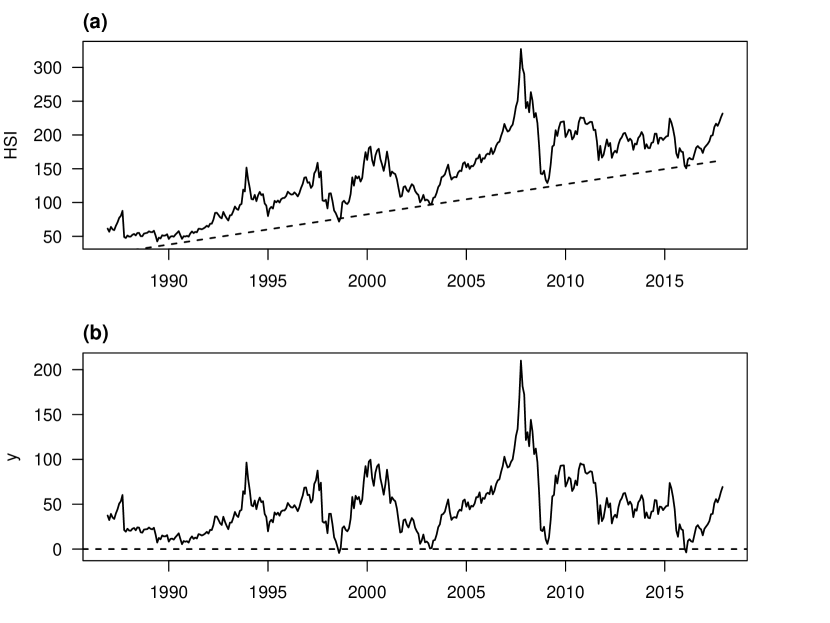
Figure 4: (a) Real HSI prices with the fitted linear trend (the dotted line); (b) $y_{t}$ series.

Thus, we first subtract such a linear trend from the series. That is, we assume that the HSI real price $x_{t}$ is decomposed into

$$x_{t}=b_{0}+b_{1}t+y_{t},$$

where $b_{0}+b_{1}t$ denotes the linear trend and $y_{t}$ follows a SNAR model. Note that $b_{i},i=0,1$ can be seen as unknown parameters and can be estimated jointly. Their estimates are $\widehat{b}_{0}=23.661$ and $\widehat{b}_{1}=0.372$, respectively. The linear time trend is plotted in Fig. 4 (a) by the dotted line and $\{y_{t}\}$ in Fig. 4 (b). The estimates with standard deviations (SDs) of the SNAR model $\{y_{t}\}$ are reported in Table 4.

Table 4: The estimate with standard deviations (SD) of the fitted SNAR model.

	$\phi_{0}$	$p_{0}$	$\sigma_{0}^{2}$
Estimate	1.026	0.977	36.314
SD	0.011	0.005	8.649

All estimates are statistically significant at the $5\%$ level since their corresponding $p$-values are extremely small which are thus not reported in the table. The estimate of $\phi_{0}$ is large than one, and its $95\%$ confidence interval is $(1.005,1.047)$, conforming to the locally explosive behavior of series $y_{t}$. For the fitting adequacy, we calculate the $p$-values of the test statistic $Q_{M}$ with $M=6,12,18$, and $24$ when the tuning parameter $a$ is the 90% or 95% quantile of $\{|y_{t}|,t=1\dots,n\}$, respectively. The results are summarized in Table 5, which implies that the fitting is adequate at the $5\%$ level.

Table 5: The $p$-values of $Q_{M}$.

$a\backslash M$	6	12	18	24
90%	0.7099	0.2427	0.3087	0.1549
95%	0.8588	0.7489	0.4898	0.1876

We then apply the bubble tagging methods described in Section 5 to label each time point as either being in a bubble state or being in the null. Since the estimated bubble probability $\widehat{p}_{0}=0.977$ from Table 4 which is very high, in view of the simulation results in Section 6, we shall here consider using the residual-based method in Section 5.1 to tag the collapses of bubbles for the series $\{y_{t}\}$. In particular, Fig. 5 displays the selected dates of $\widehat{s}_{t}=0$ under Rules 1–4. It can be seen from Fig. 5 that the tagging times can vary based on which Rule is used, but several important dates are identified simultaneously by at least two rules. Table 6 summarizes such these dates,

Table 6: The selected important dates of $s_{t}=0$.

Date	1987-10	1997-10	2008-01	2008-10	2011-09	2016-01
Rule	{1,2,3,4}	{1,2,3,4}	{1, 3}	{1,2,3,4}	{1,2}	{2,3,4}

which coinside with historical financial crises, i.e., the depression started from the Black Monday in 1987, the Asian financial crises in 1997, the global financial turmoil caused by the subprime crisis over 2007-2009, and the Hong Kong stock market plummeting in 2016.

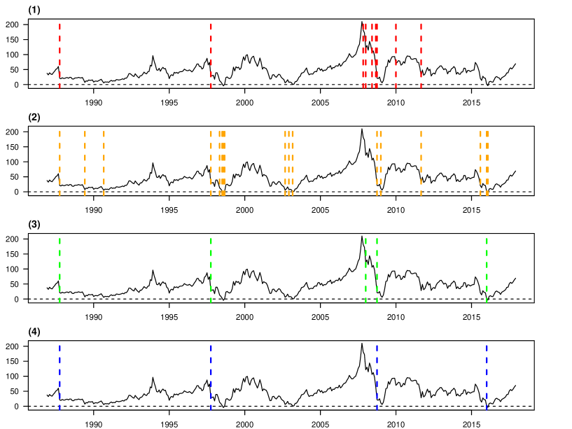
Figure 5: Selected dates of $\widehat{s}_{t}=0$ by Rules 1–4.

Although the collapse of a bubble can be dated by $\widehat{s}_{t}=0$, the emergence and exuberance of a bubble can not be asserted by $\widehat{s}_{t}=1$ immediately. After all, a short-period deviation of the price is reasonable due to the market fluctuations. Of course, a short-period deviation might be regarded as a small bubble in some sense, which bursts quickly by the market adjustment, thus we could pay little attention and ignore them afterwards. What we really need to worry about is the bubble that can trigger tremendous harm, which emerges as the accumulation of long-lasting excursion. Specifically, if $s_{t}=0,s_{t+1}=s_{t+2}=\dots=s_{t+k-1}=1,s_{t+k}=0$, then we call it an excursive period that starts from $t+1$ and ends at $t+k$, and define its duration as $k$. Within an excursive period, the presence of a bubble can be supported if the duration exceeds some time span, for example, one or two years. For our application, the time span is set to be 18 months. Table 7 summarizes the periods whose durations exceed 18 months, as well as their start and end dates.

Table 7: Excursive period with duration exceeding 18 months.

start	end	duration
1987-11	1989-06	20
1990-10	1997-10	85
1998-10	2002-09	48
2003-04	2007-11	56
2010-02	2011-09	20
2011-10	2015-08	47
2016-03	2017-12	22

Fig. 6 plots those periods by gray shadows.

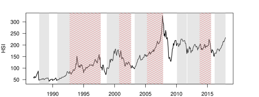
Figure 6: Excursive periods with duration exceeding 18 months shown by gray shadows; bubbles last over 24 months plotted by the shadow with red backslash.

We can see explosive behaviors in most of the periods, indicating the presence and accumulation of bubbles. By Proposition 2 in Section 5.1, the RBT method is capable of detecting the collapse of an accumulated bubble when its duration $k\to\infty$; see also the same proposition for a probabilistic bound with a finite duration. Another finding is that the magnitude of a bubble is larger as the period lasts longer possibly, for example, the one reaches a value of 210 in October 2007, corresponding to the period from April 2003 to November 2007 with the duration of 56 months. Investors should be alert to such a long-time excursion along with the potential of disastrous bubbles. In the periods where the bubble lasts over 24 months (plotted by the shadow with red backslash in Fig. 6), one should be aware of the false boom in financial markets, and adjust asset allocation to hedge the risk of a potential bubble burst.

8 Conclusions

The paper has introduced a novel stochastic nonlinear autoregressive model to describe the dynamics of economic or financial bubbles within a causal and stationary framework, and discussed its strict stationarity and geometric ergodicity. The paper has further studied the quasi-maximum likelihood estimation of the model and established the asymptotics under minimal assumptions on innovation. Due to the unobservability of the latent variable $s_{t}$ and the resulting unavailability of the residuals, a new model diagnostic checking tool has been proposed for the adequacy of the fitting. Finally, the paper considers two approaches, one from the residual perspective and the other from the null perspective, for bubble tagging.

Although our new model is useful, the model assumption on the independence between $\{\varepsilon_{t}\}$ and $\{s_{t}\}$ seems a little bit stronger from the perspective of empirical pragmatism. To obtain more reasonable interpretation or approximation of the bubble, such an independence assumption can be relaxed. For instance, we can assume that $s_{t}$ depends on the history of the observed process. Specifically, we can let $\mathbb{P}(s_{t}=1|\mathcal{F}_{t-1})=g(\bm{\beta}^{\prime}\mathbf{y}_{t-1})$, where $\mathcal{F}_{t-1}=\sigma(y_{t-j}:j\geq 1)$ be a sigma-field, $\mathbf{y}_{t-1}=(1,y_{t-1},...,y_{t-q})^{\prime}$, and $g$ is a measurable function (e.g. a logistic function). Furthermore, we can also restrict the form of $s_{t}$ in macroeconomic time series analysis and let $s_{t}=I(\bm{\beta}^{\prime}\mathbf{x}_{t}>c)$, where $\mathbf{x}_{t}$ may contain many exogenous macroeconomic variables or indexes and $c$ is a threshold parameter. In addition, it is possible to consider the situation when the hidden state process $\{s_{t}\}$ exhibits temporal dependence and forms a Markov chain. In this case, the null-based bubble tagging method in Section 5.2 can be more advantageous when bubbles occur in separated but persistent clusters. Another potential topic is to study multivariate stochastic nonlinear AR models. We leave these topics for future research.

Appendix A Technical Proofs

A.1 Proof of Theorem 1

When $\phi_{0}=0$, then $\{y_{t}\}$ reduces to an i.i.d. sequence $\{\varepsilon_{t}\}$, and in this case all results hold clearly. Without loss of generality, we assume that $\phi_{0}\neq 0$ in what follows. It suffices to verify the conditions in Theorem 19.1.3 in Meyn and Tweedie (2009). It is clear that $\{y_{t}\}$ defined by (1), with initial value $y_{0}$, is an homogeneous Markov chain on $\mathbb{R}$ endowed with its Borel $\sigma$-field $\mathcal{B}(\mathbb{R})$. Denote by $\lambda$ the Lebesgue measure on $(\mathbb{R},\mathcal{B}(\mathbb{R}))$. The transition probabilities of $\{y_{t}\}$ are given, for $y\in\mathbb{R}$, $B\in\mathcal{B}(\mathbb{R})$, by

$$\mathbf{P}(y,B)=\mathbb{P}(y_{t}\in B|y_{t-1}=y)=p_{0}\mathbb{P}(\varepsilon_{1}+\phi_{0}|y|\in B)+(1-p_{0})\mathbb{P}(\varepsilon_{1}\in B).$$

First, since $\mathbf{P}(\cdot,B)$ is continuous, for any $B\in\mathcal{B}(\mathbb{R})$, the chain $\{y_{t}\}$ has the Feller property.

Second, note that the density of $\varepsilon_{1}$ is positive over $\mathbb{R}$, we have $\mathbf{P}(y,B)>0$ whenever $\lambda(B)>0$. Thus the chain $\{y_{t}\}$ is $\lambda$-irreducible. Further, it can also be shown that the $k$-step transition probabilities $\mathbf{P}^{k}(y,B)=\mathbb{P}(y_{t}\in B|y_{t-k}=y)=\int_{\mathbb{R}}\mathbf{P}^{k-1}(x,B)\mathbf{P}(y,dx)>0$ by an inductive approach for any integer $k\geq 1$, whenever $\lambda(B)>0$, which establishes the aperiodicity of the chain $\{y_{t}\}$.

Third, let $V(x)=\log(1+|x|)$, $x\in\mathbb{R}$. Then, by a simple calculation, it follows that

$$\mathbb{E}\{V(y_{t})|y_{t-1}=y\}=(1-p_{0})\mathbb{E}\log(1+|\varepsilon_{1}|)+p_{0}\mathbb{E}\log(1+|\phi_{0}|y|+\varepsilon_{1}|).$$

Thus, we have that

$$\lim_{|y|\rightarrow\infty}\frac{\mathbb{E}\{V(y_{t})|y_{t-1}=y\}}{V(y)} =\lim_{|y|\rightarrow\infty}\frac{(1-p_{0})\mathbb{E}\log(1+|\varepsilon_{1}|)}{\log(1+|y|)}+p_{0}\lim_{|y|\rightarrow\infty}\frac{\mathbb{E}\log(1+|\phi_{0}|y|+\varepsilon_{1}|)}{\log(1+|y|)}$$

$$=0+p_{0}\lim_{|y|\rightarrow\infty}\left(\frac{\log|y|}{\log(1+|y|)}+\frac{\mathbb{E}\log\Big{(}\frac{1}{|y|}+\big{|}\phi_{0}+\frac{\varepsilon_{1}}{|y|}\big{|}\Big{)}}{\log(1+|y|)}\right)$$

$$=p_{0}.$$

Since $p_{0}\in[0,1)$, for fixed $\delta\in(0,1-p_{0})$, i.e., $p_{0}<1-\delta<1$, there exists a constant $M>0$ such that

$$\mathbb{E}\{V(y_{t})|y_{t-1}=y\}\leq(1-\delta)V(y),\quad\mbox{when $|y|>M$}.$$

To sum up the above arguments, by Theorem 19.1.3 in Meyn and Tweedie (2009), there exists a geometrically ergodic solution to model (1). The solution is unique since $\mathbb{E}\log|s_{t}\phi_{0}|=-\infty$. Thus, the results hold and then the proof is complete. $\square$

A.2 Proof of Theorem 2

Consider $\beta_{n}(\theta):=\{L_{n}(\theta)-L_{n}(\theta_{0})\}/n$, $\theta\in\Theta$. By the strong law of large numbers for stationary and ergodic sequences and the inequality $\log x+x^{-1}-1\geq 0$ for $x>0$, a conditional argument yields that

$$\beta_{n}(\theta) =\frac{1}{n}\sum_{t=1}^{n}\left\{\log\frac{p(1-p)\phi^{2}y_{t-1}^{2}+\sigma^{2}}{p_{0}(1-p_{0})\phi_{0}^{2}y_{t-1}^{2}+\sigma_{0}^{2}}+\frac{(y_{t}-p\phi|y_{t-1}|)^{2}}{p(1-p)\phi^{2}y_{t-1}^{2}+\sigma^{2}}-\frac{(y_{t}-p_{0}\phi_{0}|y_{t-1}|)^{2}}{p_{0}(1-p_{0})\phi_{0}^{2}y_{t-1}^{2}+\sigma_{0}^{2}}\right\}$$

$$\stackrel{{\scriptstyle\mathrm{a.s.}}}{{\longrightarrow}}\mathbb{E}\left\{\log\frac{p(1-p)\phi^{2}y_{t-1}^{2}+\sigma^{2}}{p_{0}(1-p_{0})\phi_{0}^{2}y_{t-1}^{2}+\sigma_{0}^{2}}+\frac{(y_{t}-p\phi|y_{t-1}|)^{2}}{p(1-p)\phi^{2}y_{t-1}^{2}+\sigma^{2}}-\frac{(y_{t}-p_{0}\phi_{0}|y_{t-1}|)^{2}}{p_{0}(1-p_{0})\phi_{0}^{2}y_{t-1}^{2}+\sigma_{0}^{2}}\right\}$$

$$=\mathbb{E}\left\{\log\frac{p(1-p)\phi^{2}y_{t-1}^{2}+\sigma^{2}}{p_{0}(1-p_{0})\phi_{0}^{2}y_{t-1}^{2}+\sigma_{0}^{2}}+\frac{p_{0}(1-p_{0})\phi_{0}^{2}y_{t-1}^{2}+\sigma_{0}^{2}}{p(1-p)\phi^{2}y_{t-1}^{2}+\sigma^{2}}-1+\frac{(p\phi-p_{0}\phi_{0})^{2}y_{t-1}^{2}}{p(1-p)\phi^{2}y_{t-1}^{2}+\sigma^{2}}\right\}\geq 0,$$

where the equality holds if and only if

$$p(1-p)\phi^{2}y_{t-1}^{2}+\sigma^{2}=p_{0}(1-p_{0})\phi_{0}^{2}y_{t-1}^{2}+\sigma_{0}^{2}\quad\mbox{and}\quad(p\phi-p_{0}\phi_{0})^{2}=0\quad\mbox{a.s.},$$

equivalently, $\left\{p(1-p)\phi^{2}-p_{0}(1-p_{0})\phi_{0}^{2}\right\}y_{t-1}^{2}=\sigma_{0}^{2}-\sigma^{2}$ a.s. Then

$$p(1-p)\phi^{2}-p_{0}(1-p_{0})\phi_{0}^{2}=0,\quad\sigma_{0}^{2}-\sigma^{2}=0.$$

Combining with $(p\phi-p_{0}\phi_{0})^{2}=0$, we have $\phi=\phi_{0}$, $p=p_{0}$ and $\sigma^{2}=\sigma_{0}^{2}$, i.e., $\theta=\theta_{0}$. The remainder of the proof can be completed by a standard compactness argument and it is thus omitted. $\square$

A.3 Proof of Theorem 3

Let $q_{t}(\theta)=p(1-p)\phi^{2}y_{t-1}^{2}+\sigma^{2}$ and $q_{t}:=q_{t}(\theta_{0})$. Then the first- and second-order partial derivatives of $q_{t}(\theta)$ with respect to $\theta$ are respectively as follows

$$\frac{\partial q_{t}(\theta)}{\partial\theta}=\left(\begin{array}[]{c}2p(1-p)\phi y_{t-1}^{2}\\ (1-2p)\phi^{2}y_{t-1}^{2}\\ 1\end{array}\right),\quad\frac{\partial^{2}q_{t}(\theta)}{\partial\theta\partial\theta^{\prime}}=\left(\begin{array}[]{ccc}2p(1-p)y_{t-1}^{2}&2(1-2p)\phi y_{t-1}^{2}&0\\ &-2\phi^{2}y_{t-1}^{2}&0\\ &&0\end{array}\right).$$ (14)

Using the notation $q_{t}(\theta)$, we have

$$\ell_{t}(\theta)=\log\left[q_{t}(\theta)\right]+\frac{(y_{t}-p\phi|y_{t-1}|)^{2}}{q_{t}(\theta)}.$$

A simple calculation yields the first-order partial derivatives of $\ell_{t}(\theta)$ with respect to $\theta$

$$\frac{\partial\ell_{t}(\theta)}{\partial\theta} =\frac{1}{q_{t}(\theta)}\frac{\partial q_{t}(\theta)}{\partial\theta}-\frac{2|y_{t-1}|(y_{t}-p\phi|y_{t-1}|)}{q_{t}(\theta)}\vartheta-\frac{(y_{t}-p\phi|y_{t-1}|)^{2}}{\left[q_{t}(\theta)\right]^{2}}\frac{\partial q_{t}(\theta)}{\partial\theta},$$ (15)

where $\vartheta=(p,\phi,0)^{\prime}$, and the second-order partial derivatives

$$\frac{\partial^{2}\ell_{t}(\theta)}{\partial\theta\partial\theta^{\prime}} =\left\{\frac{1}{q_{t}(\theta)}-\frac{(y_{t}-p\phi|y_{t-1}|)^{2}}{[q_{t}(\theta)]^{2}}\right\}\frac{\partial^{2}q_{t}(\theta)}{\partial\theta\partial\theta^{\prime}}+\left\{\frac{2(y_{t}-p\phi|y_{t-1}|)^{2}}{[q_{t}(\theta)]^{3}}-\frac{1}{[q_{t}(\theta)]^{2}}\right\}\frac{\partial q_{t}(\theta)}{\partial\theta}\frac{\partial q_{t}(\theta)}{\partial\theta^{\prime}}$$

$$\quad+\frac{2|y_{t-1}|(y_{t}-p\phi|y_{t-1}|)}{[q_{t}(\theta)]^{2}}\left\{\frac{\partial q_{t}(\theta)}{\partial\theta}\vartheta^{\prime}+\vartheta\frac{\partial q_{t}(\theta)}{\partial\theta^{\prime}}\right\}+\frac{2y_{t-1}^{2}}{q_{t}(\theta)}\vartheta\vartheta^{\prime}$$

$$\quad-\frac{2|y_{t-1}|(y_{t}-p\phi|y_{t-1}|)}{q_{t}(\theta)}\begin{bmatrix}0&1&0\\ 1&0&0\\ 0&0&0\end{bmatrix}.$$

By the Taylor expansion, by the definition of $\widehat{\theta}_{n}$, we have

$$0=\frac{1}{\sqrt{n}}\frac{\partial L_{n}(\widehat{\theta}_{n})}{\partial\theta}=\frac{1}{\sqrt{n}}\frac{\partial L_{n}(\theta_{0})}{\partial\theta}+\frac{1}{n}\frac{\partial^{2}L_{n}(\theta^{*})}{\partial\theta\partial\theta^{\prime}}\sqrt{n}\big{(}\widehat{\theta}_{n}-\theta_{0}\big{)},$$

where $\theta^{*}\in\Theta$ and satisfies $\|\theta^{*}-\theta_{0}\|\leq\|\widehat{\theta}_{n}-\theta_{0}\|$. Note that the continuity of $\partial^{2}\ell_{t}(\theta)/\partial\theta\partial\theta^{\prime}$ in $\theta$ and the strong law of large numbers for stationary and ergodic sequences, it is not hard to get

$$\frac{1}{n}\frac{\partial^{2}L_{n}(\theta^{*})}{\partial\theta\partial\theta^{\prime}}=\frac{1}{n}\frac{\partial^{2}L_{n}(\theta_{0})}{\partial\theta\partial\theta^{\prime}}+o_{p}(1)=\mathcal{J}+o_{p}(1).$$

Further, let $\mathcal{F}_{t}=\sigma(y_{j}:j\leq t)$ be the $\sigma$-algebra generated by the random variables $\{y_{j}:j\leq t\}$. By the expressions in (14) and (15), and the following facts

$$\begin{split}\mathbb{E}[y_{t}-p_{0}\phi_{0}|y_{t-1}||\mathcal{F}_{t-1}]&=\mathbb{E}[(s_{t}-p_{0})\phi_{0}|y_{t-1}|+\varepsilon_{t}|\mathcal{F}_{t-1}]=0,\\ \mathbb{E}[(y_{t}-p_{0}\phi_{0}|y_{t-1}|)^{2}|\mathcal{F}_{t-1}]&=p_{0}(1-p_{0})\phi^{2}_{0}y_{t-1}^{2}+\sigma^{2}_{0}=q_{t},\end{split}$$ (16)

we have that

$$\mathbb{E}\Big{\{}\frac{\partial\ell_{t}(\theta_{0})}{\partial\theta}\Big{|}\mathcal{F}_{t-1}\Big{\}}=0,$$

i.e., $\{\partial\ell_{t}(\theta_{0})/\partial\theta\}$ is a martingale difference sequence with respect to $\{\mathcal{F}_{t}\}$. Thus, by the martingale central limit theorem in Brown (1971), it follows that

$$\frac{1}{\sqrt{n}}\frac{\partial L_{n}(\theta_{0})}{\partial\theta}=\frac{1}{\sqrt{n}}\sum_{t=1}^{n}\frac{\partial\ell_{t}(\theta_{0})}{\partial\theta}\stackrel{{\scriptstyle d}}{{\longrightarrow}}\mathcal{N}(0,\mathcal{I}),$$

where

$$\mathcal{I}=\mathbb{E}\left\{\frac{\partial\ell_{t}(\theta_{0})}{\partial\theta}\frac{\partial\ell_{t}(\theta_{0})}{\partial\theta^{\prime}}\right\}.$$ (17)

Finally, we have

$$\sqrt{n}\big{(}\widehat{\theta}_{n}-\theta_{0}\big{)}=-[\mathcal{J}+o_{p}(1)]^{-1}\frac{1}{\sqrt{n}}\frac{\partial L_{n}(\theta_{0})}{\partial\theta}\stackrel{{\scriptstyle d}}{{\longrightarrow}}\mathcal{N}(0,\mathcal{J}^{-1}\mathcal{I}\mathcal{J}^{-1}).$$ (18)

As for the explicit expressions of $\mathcal{I}$ and $\mathcal{J}$, by (14), (16), and the following facts

$$\mathbb{E}[(y_{t}-p_{0}\phi_{0}|y_{t-1}|)^{3}|\mathcal{F}_{t-1}] =p_{0}(1-p_{0})(1-2p_{0})\phi_{0}^{3}|y_{t-1}|^{3}+\kappa_{3},$$

$$\mathbb{E}[(y_{t}-p_{0}\phi_{0}|y_{t-1}|)^{4}|\mathcal{F}_{t-1}] =p_{0}(1-p_{0})(1-3p_{0}+3p_{0}^{2})\phi_{0}^{4}y_{t-1}^{4}+6\sigma_{0}^{2}p_{0}(1-p_{0})\phi_{0}^{2}y_{t-1}^{2}+\kappa_{4},$$

a tedious algebraic calculation can yield them and the detail is omitted. The proof is complete. $\square$

A.4 Proof of Theorem 4

According to the definition of $\widehat{\eta}_{t}$, by Theorem 2 and the strong law of large numbers for a stationary and ergodic sequence, we first have the following facts, as $n\rightarrow\infty$,

$$\bar{\eta} =\phi_{0}\frac{1}{n}\sum_{t=1}^{n}(s_{t}-p_{0})|y_{t-1}|I(|y_{t-1}|\leq a)+\frac{1}{n}\sum_{t=1}^{n}\varepsilon_{t}I(|y_{t-1}|\leq a)$$

$$\qquad+(p_{0}\phi_{0}-\widehat{p}_{n}\widehat{\phi}_{n})\frac{1}{n}\sum_{t=1}^{n}|y_{t-1}|I(|y_{t-1}|\leq a)$$

$$\stackrel{{\scriptstyle a.s.}}{{\rightarrow}}\phi_{0}\mathbb{E}(s_{t}-p_{0})\mathbb{E}[|y_{t-1}|I(|y_{t-1}|\leq a)]+(\mathbb{E}\varepsilon_{t})\mathbb{P}(|y_{t-1}|\leq a)+0\cdot\mathbb{E}[|y_{t-1}|I(|y_{t-1}|\leq a)]=0$$

and

$$\frac{1}{n}\sum_{t=1}^{n}(\widehat{\eta}_{t}-\bar{\eta})^{2} =\frac{1}{n}\sum_{t=1}^{n}\widehat{\eta}_{t}^{2}-\bar{\eta}^{2}$$

$$=\phi_{0}^{2}\frac{1}{n}\sum_{t=1}^{n}(s_{t}-p_{0})^{2}y_{t-1}^{2}I(|y_{t-1}|\leq a)+\frac{1}{n}\sum_{t=1}^{n}\varepsilon_{t}^{2}I(|y_{t-1}|\leq a)$$

$$\quad+(p_{0}\phi_{0}-\widehat{p}_{n}\widehat{\phi}_{n})^{2}\frac{1}{n}\sum_{t=1}^{n}y_{t-1}^{2}I(|y_{t-1}|\leq a)$$

$$\quad+2\phi_{0}\frac{1}{n}\sum_{t=1}^{n}(s_{t}-p_{0})\varepsilon_{t}|y_{t-1}|I(|y_{t-1}|\leq a)$$

$$\quad+2\phi_{0}(p_{0}\phi_{0}-\widehat{p}_{n}\widehat{\phi}_{n})\frac{1}{n}\sum_{t=1}^{n}(s_{t}-p_{0})y^{2}_{t-1}I(|y_{t-1}|\leq a)$$ (19)

$$\quad+2(p_{0}\phi_{0}-\widehat{p}_{n}\widehat{\phi}_{n})\frac{1}{n}\sum_{t=1}^{n}\varepsilon_{t}|y_{t-1}|I(|y_{t-1}|\leq a)$$

$$\stackrel{{\scriptstyle a.s.}}{{\rightarrow}}p_{0}(1-p_{0})\phi_{0}^{2}\mathbb{E}\{y_{t-1}^{2}I(|y_{t-1}|\leq a)\}+\sigma_{0}^{2}\mathbb{P}(|y_{t-1}|\leq a)=\sigma_{\eta}^{2},$$

where $\sigma_{\eta}^{2}$ is defined in (3). Further, using the preceding expression of $\bar{\eta}$, we have that $\bar{\eta}=O_{p}(1/\sqrt{n})$ by the martingale central limit theorem in Brown (1971) and Theorems 2-3. Similarly, we can get

$$\frac{1}{n}\sum_{t=k+1}^{n}(\widehat{\eta}_{t}-\bar{\eta})(\widehat{\eta}_{t-k}-\bar{\eta})-\frac{1}{n}\sum_{t=k+1}^{n}\widehat{\eta}_{t}\widehat{\eta}_{t-k}=\frac{n-k}{n}\bar{\eta}^{2}-\bar{\eta}\frac{1}{n}\sum_{t=k+1}^{n}\widehat{\eta}_{t}-\bar{\eta}\frac{1}{n}\sum_{t=k+1}^{n}\widehat{\eta}_{t-k}=O_{p}(1/n)$$

for each fixed $k\geq 0$. Using above facts, we have that

$$\sqrt{n}\widehat{\rho}_{nk}=(1+o_{p}(1))\left\{\frac{1}{\sigma_{\eta}^{2}\sqrt{n}}\sum_{t=k+1}^{n}\widehat{\eta}_{t}\widehat{\eta}_{t-k}\right\}+o_{p}(1).$$ (20)

Next, it suffices to consider the joint limiting distribution of $(\sigma_{\eta}^{2}\sqrt{n})^{-1}\sum_{t=k+1}^{n}\widehat{\eta}_{t}\widehat{\eta}_{t-k}$, $k=1,...,M$. To this end, let $\eta_{t}(\theta)=(y_{t}-p\phi|y_{t-1}|)I(|y_{t-1}|\leq a)$, then $\widehat{\eta}_{t}=\eta_{t}(\widehat{\theta}_{n})$ and $\eta_{t}=\eta_{t}(\theta_{0})$ in (2). Denote

$$\rho_{nk}(\theta)=\frac{1}{n\sigma_{\eta}^{2}}\sum_{t=k+1}^{n}\eta_{t}(\theta)\,\eta_{t-k}(\theta),\quad\theta\in\Theta,\quad k\geq 1.$$

Note that $\partial\eta_{t}(\theta)/\partial\theta=-\vartheta|y_{t-1}|I(|y_{t-1}|\leq a)$, where $\vartheta=(p,\phi,0)^{\prime}$, and

$$\frac{\partial\rho_{nk}(\theta_{0})}{\partial\theta^{\prime}} =\frac{1}{n\sigma_{\eta}^{2}}\sum_{t=k+1}^{n}\frac{\partial\eta_{t}(\theta_{0})}{\partial\theta^{\prime}}\,\eta_{t-k}+\frac{1}{n\sigma_{\eta}^{2}}\sum_{t=k+1}^{n}\eta_{t}\frac{\partial\eta_{t-k}(\theta_{0})}{\partial\theta^{\prime}}$$

$$=-\vartheta_{0}^{\prime}\left\{\frac{1}{n\sigma_{\eta}^{2}}\sum_{t=k+1}^{n}\eta_{t-k}|y_{t-1}|I(|y_{t-1}|\leq a)+\frac{1}{n\sigma_{\eta}^{2}}\sum_{t=k+1}^{n}\eta_{t}|y_{t-k-1}|I(|y_{t-k-1}|\leq a)\right\}$$

$$=\frac{u_{k}}{\sigma_{\eta}^{2}}\vartheta_{0}^{\prime}+o_{p}(1)$$

with $u_{k}=-\mathbb{E}\{\eta_{t-k}|y_{t-1}|I(|y_{t-1}|\leq a)$, by the law of large numbers and $\mathbb{E}\eta_{t}=0$. Then, by the Taylor expansion, the law of large numbers, and Theorems 2-3, it follows that

$$\sqrt{n}\big{(}\rho_{nk}(\widehat{\theta}_{n})-\rho_{nk}(\theta_{0})\big{)}=\frac{\partial\rho_{nk}(\theta_{0})}{\partial\theta^{\prime}}\sqrt{n}(\widehat{\theta}_{n}-\theta_{0})+o_{p}(1)=\frac{u_{k}}{\sigma_{\eta}^{2}}\vartheta_{0}^{\prime}\sqrt{n}(\widehat{\theta}_{n}-\theta_{0})+o_{p}(1).$$

Let ${\bm{\rho}}_{n}(\theta)=(\rho_{n1}(\theta),...,\rho_{nM}(\theta))^{\prime}$. It follows that

$$\sqrt{n}{\bm{\rho}}_{n}(\widehat{\theta}_{n})=\sqrt{n}{\bm{\rho}}_{n}(\theta_{0})+\frac{1}{\sigma_{\eta}^{2}}\left(\begin{array}[]{c}u_{1}\\ \vdots\\ u_{M}\end{array}\right)\vartheta_{0}^{\prime}\sqrt{n}(\widehat{\theta}_{n}-\theta_{0})+o_{p}(1).$$

By (18), we have

$$\sqrt{n}(\widehat{\theta}_{n}-\theta_{0})=-\mathcal{J}^{-1}\frac{1}{\sqrt{n}}\sum_{t=1}^{n}\frac{\partial\ell_{t}(\theta_{0})}{\partial\theta}+o_{p}(1).$$

The martingale central limit theorem in Brown (1971) gives that

$$\left(\begin{array}[]{c}\sqrt{n}{\bm{\rho}}_{n}(\theta_{0})\\ \sqrt{n}(\widehat{\theta}_{n}-\theta_{0})\end{array}\right)\stackrel{{\scriptstyle d}}{{\longrightarrow}}\mathcal{N}(0,\mathbf{G}).$$

Thus, $\sqrt{n}{\bm{\rho}}_{n}(\widehat{\theta}_{n})\stackrel{{\scriptstyle d}}{{\longrightarrow}}\ \mathcal{N}(0,\mathbf{UGU}^{\prime})$ by a matrix linear transformation.

Finally, note that, by (A.4)-(20),

$$\sqrt{n}\big{(}\widehat{\bm{\rho}}_{n}-{\bm{\rho}}_{n}(\widehat{\theta}_{n})\big{)}=o_{p}(1)\sqrt{n}{\bm{\rho}}_{n}(\widehat{\theta}_{n})+o_{p}(1)=o_{p}(1)O_{p}(1)+o_{p}(1)=o_{p}(1).$$

Thus, $\sqrt{n}\widehat{\bm{\rho}}_{n}\stackrel{{\scriptstyle d}}{{\longrightarrow}}\mathcal{N}(0,\mathbf{UGU}^{\prime})$. The proof is complete. $\square$

A.5 Proof of Proposition 1

For any time point $t$, a $k$-th cumulative bubble collapses if $s_{t}=0$, $s_{t-l}=1$ for $1\leq l\leq k$ and $s_{t-k-1}=0$. Let $\{z_{s}^{\diamond}\}$ be a new auxiliary process that satisfies the recursion

$$z_{s}^{\diamond}=\left\{\begin{array}[]{ll}\varepsilon_{s},&\mbox{if $s\leq t-k-1$},\\ \phi_{0}|z_{s-1}^{\diamond}|+\varepsilon_{s},&\mbox{if $s>t-k-1$},\end{array}\right.$$

then $y_{t-1}=z_{t-1}^{\diamond}$ if a $k$-th cumulative bubble is formed at time $t-1$ to be collapsed at time $t$. Note that the process $\{z_{s}^{\diamond}\}$ is constructed using the innovation sequence $\{\varepsilon_{t}\}$, which is independent of the sequence $\{s_{t}\}$, we can show that the joint probability

$$\mathbb{P}(r_{t}\leq c_{r},s_{t}=0,s_{t-1}=\cdots=s_{t-k}=1,s_{t-k-1}=0)$$

$$=\ \mathbb{P}(\varepsilon_{t}-\phi_{0}|z_{t-1}^{\diamond}|\leq c_{r},s_{t}=0,s_{t-1}=\cdots=s_{t-k}=1,s_{t-k-1}=0)$$

$$=\ p_{0}^{k}(1-p_{0})^{2}\mathbb{P}(\varepsilon_{t}-\phi_{0}|z_{t-1}^{\diamond}|\leq c_{r}).$$

On the other hand, the marginal probability that a $k$-th cumulative bubble collapses at time $t$ equals to $\mathbb{P}(s_{t}=0,s_{t-1}=\cdots=s_{t-k}=1,s_{t-k-1}=0)=p_{0}^{k}(1-p_{0})^{2}$, and thus it suffices to show that

$$\mathbb{P}(\varepsilon_{t}-\phi_{0}|z_{t-1}^{\diamond}|\leq c_{r})=\mathbb{P}(z_{k}\geq-c_{r}).$$

For this, note that the two vectors $(\varepsilon_{t-k},\ldots,\varepsilon_{t})$ and $(\varepsilon_{0},\ldots,\varepsilon_{k})$ share the same distribution, and thus by definition the two vectors $(z_{t-1}^{\diamond},\ldots,z_{t-k-1}^{\diamond})$ and $(z_{k},\ldots,z_{0})$ have the same joint distribution. By independence of $\varepsilon_{t}$ and $z_{t-1}^{\diamond}$ we can then conclude that

$$\mathbb{P}(\varepsilon_{t}-\phi_{0}|z_{t-1}^{\diamond}|\leq c_{r})=\mathbb{P}(\varepsilon_{k}-\phi_{0}|z_{k-1}|\leq c_{r})=\mathbb{P}(\phi_{0}|z_{k-1}|-\varepsilon_{k}\geq-c_{r}).$$

If the innovation sequence $\{\varepsilon_{t}\}$ has a symmetric distribution, then $z_{k}=\phi_{0}|z_{k-1}|+\varepsilon_{k}$ has the same distribution as $\phi_{0}|z_{k-1}|-\varepsilon_{k}$, and the result follows. $\square$

A.6 Proof of Proposition 2

For any time point $t$, it constitutes a $k$-th cumulative bubble if $s_{t-l}=1$ for $0\leq l\leq k-1$ and $s_{t-k}=0$. Let $\{z_{s}^{\circ}\}$ be a new auxiliary process that satisfies the recursion

$$z_{s}^{\circ}=\left\{\begin{array}[]{ll}\varepsilon_{s},&\mbox{if $s\leq t-k$},\\ \phi_{0}|z_{s-1}^{\circ}|+\varepsilon_{s},&\mbox{if $s>t-k$},\end{array}\right.$$

then by the independence of $\{\varepsilon_{t}\}$ and $\{s_{t}\}$ we can show that the joint probability

$$\mathbb{P}(y_{t}>c,s_{t}=\cdots=s_{t-k+1}=1,s_{t-k}=0) =\mathbb{P}(z_{t}^{\circ}>c,s_{t}=\cdots=s_{t-k+1}=1,s_{t-k}=0)$$

$$=\mathbb{P}(z_{t}^{\circ}>c)\cdot\mathbb{P}(s_{t}=\cdots=s_{t-k+1}=1,s_{t-k}=0)$$

$$=p_{0}^{k}(1-p_{0})\mathbb{P}(z_{t}^{\circ}>c).$$

On the other hand, the marginal probability that time $t$ is a $k$-th cumulative bubble equals to $\mathbb{P}(s_{t}=\cdots=s_{t-k+1}=1,s_{t-k}=0)=p_{0}^{k}(1-p_{0})$, and thus it suffices to show that $\{z_{s}^{\circ}\}_{t-k<s\leq t}$ and $\{z_{s^{\prime}}\}_{1\leq s^{\prime}\leq k}$ share the same distribution. For this, note that the two vectors $(\varepsilon_{t-k},\ldots,\varepsilon_{t})$ and $(\varepsilon_{0},\ldots,\varepsilon_{k})$ share the same distribution, and they drive $z_{s}^{\circ}$, $t-k<s\leq t$, and $z_{s^{\prime}}$, $1\leq s^{\prime}\leq k$, based on the same recursion, the result then follows. $\square$

References

- Blanchard and Watson (1982) Blanchard, O. J. and M. W. Watson (1982). Bubbles, rational expectations and financial markets. in: Wachter, Paul (Ed.), Crises in the Economic and Financial Structure. Lexington Books, Lexington, MA. pp. 295–315.
- Blasques et al. (2022) Blasques, F., S. J. Koopman, and M. Nientker (2022). A time-varying parameter model for local explosions. J. Econometrics 227, 65–84.
- Brockwell and Davis (1991) Brockwell, P. J. and R. A. Davis (1991). Time Series: Theory and Methods (2nd ed.). Springer-Verlag, New York.
- Brown (1971) Brown, B. M. (1971). Martingale central limit theorems. Ann. Math. Statist. 42, 59–66.
- Cavaliere et al. (2020) Cavaliere, G., H. B. Nielsen, and A. Rahbek (2020). Bootstrapping noncausal autoregressions: With applications to explosive bubble modeling. J. Bus. Econom. Statist. 38(1), 55–67.
- Chen and Zhu (2015) Chen, M. and K. Zhu (2015). Sign-based portmanteau test for ARCH-type models with heavy-tailed innovations. J. Econometrics 189(2), 313–320.
- Davis and Song (2020) Davis, R. A. and L. Song (2020). Noncausal vector AR processes with application to economic time series. J. Econometrics 216(1), 246–267.
- Diba and Grossman (1988a) Diba, B. T. and H. I. Grossman (1988a). Explosive rational bubbles in stock prices? Am. Econ. Rev. 78(3), 520–530.
- Diba and Grossman (1988b) Diba, B. T. and H. I. Grossman (1988b). The theory of rational bubbles in stock prices. The Economic Journal 98(392), 746–754.
- Esteve and Prats (2023) Esteve, V. and M. A. Prats (2023). Testing explosive bubbles with time-varying volatility: The case of spanish public debt. Finance Research Letters 51, 103330.
- Evans (1991) Evans, G. W. (1991). Pitfalls in testing for explosive bubbles in asset prices. Am. Econ. Rev. 81(4), 922–930.
- Fries (2022) Fries, S. (2022). Conditional moments of noncausal alpha-stable processes and the prediction of bubble crash odds. J. Bus. Econom. Statist. 40(4), 1596–1616.
- Fries and Zakoïan (2019) Fries, S. and J.-M. Zakoïan (2019). Mixed causal-noncausal AR processes and the modelling of explosive bubbles. Econom. Theory 35(6), 1234–1270.
- Gouriéroux and Jasiak (2016) Gouriéroux, C. and J. Jasiak (2016). Filtering, prediction and simulation methods for noncausal processes. J. Time Series Anal. 37(3), 405–430.
- Gouriéroux and Zakoïan (2017) Gouriéroux, C. and J.-M. Zakoïan (2017). Local explosion modelling by non-causal process. J. R. Stat. Soc. Ser. B. Stat. Methodol. 79(3), 737–756.
- Harvey et al. (2019) Harvey, D. I., S. J. Leybourne, and Y. Zu (2019). Testing explosive bubbles with time-varying volatility. Econom. Rev. 38(10), 1131–1151.
- Harvey et al. (2020) Harvey, D. I., S. J. Leybourne, and Y. Zu (2020). Sign-based unit root tests for explosive financial bubbles in the presence of deterministically time-varying volatility. Econom. Theory 36(1), 122–169.
- Johansen and Lange (2013) Johansen, S. and T. Lange (2013). Least squares estimation in a simple random coefficient autoregressive model. J. Econometrics 177(2), 285–288.
- Kurozumi and Skrobotov (2023) Kurozumi, E. and A. Skrobotov (2023). On the asymptotic behavior of bubble date estimators. J. Time Series Anal. 44(4), 359–373.
- Kurozumi et al. (2022) Kurozumi, E., A. Skrobotov, and A. Tsarev (2022). Time-transformed test for bubbles under non-stationary volatility. J. Financial Econom.. (In Press).
- Lanne and Saikkonen (2011) Lanne, M. and P. Saikkonen (2011). Noncausal autoregressions for economic time series. J. Time Ser. Econom. 3(3), Art. 2, 32.
- Li and Tong (2020) Li, D. and H. Tong (2020). On an absolute autoregressive model and skew symmetric distributions. Statistica 80(2), 177–198.
- Li (2004) Li, W. K. (2004). Diagnostic Checks in Time Series. Chapman & Hall/CRC.
- Li and Mak (1994) Li, W. K. and T. K. Mak (1994). On the least squared residual autocorrelations in non-linear times series with conditional heterscedasticity. J. Time Series Anal. 15(6), 627–636.
- Ling (2005) Ling, S. (2005). Self-weighted least absolute deviation estimation for infinite variance autoregressive models. J. R. Stat. Soc. Ser. B Stat. Methodol. 67(3), 381–393.
- Ling (2007) Ling, S. (2007). Self-weighted and local quasi-maximum likelihood estimators for ARMA-GARCH/IGARCH models. J. Econometrics 140(2), 849–873.
- McLeod and Li (1983) McLeod, A. I. and W. K. Li (1983). Diagnostic checking ARMA time series models using squared-residual autocorrelations. J. Time Series Anal. 4(4), 269–273.
- Meyn and Tweedie (2009) Meyn, S. and R. L. Tweedie (2009). Markov Chains and Stochastic Stability (2nd ed.). Cambridge University Press, Cambridge.
- Nicholls and Quinn (1982) Nicholls, D. F. and B. G. Quinn (1982). Random Coefficient Autoregressive Models: An Introduction. Springer, New York.
- Phillips et al. (2015a) Phillips, P. C. B., S. Shi, and J. Yu (2015a). Testing for multiple bubbles: Historical episodes of exuberance and collapse in the S&P 500. Internat. Econom. Rev. 56(4), 1043–1078.
- Phillips et al. (2015b) Phillips, P. C. B., S. Shi, and J. Yu (2015b). Testing for multiple bubbles: Limit theory of real-time detectors. Internat. Econom. Rev. 56(4), 1079–1133.
- Phillips et al. (2011) Phillips, P. C. B., Y. Wu, and J. Yu (2011). Explosive behavior in the 1990s Nasdaq: When did exuberance escalate asset values? Internat. Econom. Rev. 52(1), 201–226.
- Phillips and Yu (2011) Phillips, P. C. B. and J. Yu (2011). Dating the timeline of financial bubbles during the subprime crisis. Quant. Econ. 2(3), 455–491.
- Tao et al. (2019) Tao, Y., P. C. B. Phillips, and J. Yu (2019). Random coefficient continuous systems: Testing for extreme sample path behavior. J. Econometrics 209(2), 208–237.
- Tong (1990) Tong, H. (1990). Non-Linear Time Series: A Dynamical System Approach. Oxford University Press, New York.