MedTransformer: Accurate Alzheimer’s Disease Diagnosis for 3D MRI Images through 2D Vision Transformers

Abstract

Automated diagnosis of Alzheimer’s Disease (AD) in brain images is becoming a clinically important technique to support precision and efficient diagnosis and treatment planning. A few efforts have been made to automatically diagnose AD in magnetic resonance imaging (MRI) using three-dimensional CNNs. However, due to the complexity of 3D models, the performance is still unsatisfactory, both in terms of accuracy and efficiency. To overcome the complexities of 3D images and 3D models, in this study, we aim to attack this problem with 2D vision Transformers. We propose a 2D transformer-based medical image model with various transformer attention encoders to diagnose Alzheimer’s disease (AD) in 3D MRI images, by cutting the 3D images into multiple 2D slices. The model consists of four main components: shared encoders across three dimensions, dimension-specific encoders, attention across images from the same dimension, and attention across three dimensions. It is used to obtain attention relationships among multiple sequences from different dimensions (axial, coronal, and sagittal) and multiple slices. We also propose morphology augmentation, an erosion and dilation based method to increase the structural difference between AD and normal images. In this experiment, we use multiple datasets from ADNI, AIBL, MIRAID, OASIS to show the performance of our model. Our proposed MedTransformer demonstrates a strong ability in diagnosing AD. These results demonstrate the effectiveness of MedTransformer in learning from 3D data using a much smaller model and its capability to generalize among different medical tasks, which provides a possibility to help doctors diagnose AD in a simpler way.

1 Introduction

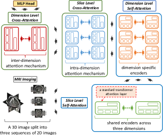
Figure 1: The overall framework of our proposed 2D ViT-Based Model for 3D Medical Imaging (MedTransformer).

Alzheimer’s disease (AD) is a highly common neurodegenerative disorder that is usually diagnosed by structural alterations of the brain mass. Therefore, investigating the structural changes in the brain is usually a critical step in diagnosing AD. To study the structural changes, the physicians usually need to read slices of brain images, typically magnetic resonance imaging (MRI), from the patients and study the structural alterations.

However, the analysis of large and intricate MRI images and the manual extraction of crucial information can pose challenges for physicians. Furthermore, the time-consuming nature of manually analyzing brain 3D MRI, coupled with potential inter- or intra-operator variability issues, increases the vulnerability to misdiagnosis [10]. Therefore, the community has been using machine intelligence to help physicians diagnose AD diseases [28]. In recent years, Convolutional Neural Networks (CNN) have been established with a dominant performance in the medical imaging field [38, 13], due to their effectiveness in extracting meaningful spatial hierarchical features from complex image data.

At the same time, transformers and self-attention mechanisms [45] have gradually surpassed CNNs, becoming a trend in the deep learning arena. The Vision Transformer [12] first demonstrated the effective application of transformer networks to image processing, achieving impressive results. Subsequently, transformer networks have gained widespread adoption in computer vision tasks, including image classification [6], object detection [5], and segmentation [49]. Additionally, ViT shows performance on par with traditional CNN-based methods for extensive databases, presenting the transformer model as a viable competitor to other advanced techniques. However, its performance is less convincing on smaller datasets compared to CNN models. A primary reason is that due to a lack of inductive bias of locality, lower layers of ViT can not learn the local relations well, leading to the representation being unreliable [57]. Moreover, in 3D medical imaging, the scarcity of datasets, largely due to ethical considerations that restrict access [39, 41], costly annotations [54, 50], class imbalance challenges [52], and the significant computational demands of processing high-dimensional data [42], is a notable issue. As a result, purely transformer-based methods have yet to see widespread use in 3D medical image diagnosis.

In addition, CNNs often struggle with high-dimensional data due to their limited receptive field [31, 12]. On the other hand, transformer models, through their self-attention mechanisms, analyze relationships between all elements in the input sequence simultaneously. This capability enables transformers to effectively capture global context and dependencies, proving advantageous in tasks requiring long-range interaction analysis. Such spatial relationships are crucial in 3D MRI images for Alzheimer’s diagnosis [26], where understanding cross-sectional interdependencies is the key.

However, vision transformers are facing new challenges when the data are 3D images. With increased spatial dimensions, the self-attention mechanism demands significantly more computational resources, which can lead to suboptimal outcomes. Some works, such as Axial-DeepLab [47], address this by factorizing 2D attention into two 1D attentions along the height and width axes, sequentially improving results. Moreover, the challenge of overfitting is exacerbated in 3D MRI image analysis. This is primarily due to 3D models having considerably more parameters than their 2D counterparts, posing difficulties in training with the limited medical data available.

Inspired by the problems mentioned above, we propose MedTransformer, a pure transformer-based model that factorizes 3D MRI images into three 2D sequences of slices along axial, coronal and sagittal dimensions. Our goal is to classify Alzheimer’s disease (AD) and normal states in 3D MRI images. The overall architecture of the proposed MedTransformer model is shown in Fig 1. Similar to [27], we also combine multi 2D slices as input and use transformer models to classify. However, unlike their model, which uses 3D+2D CNNs to extract the features among the same dimension, we directly use 2D separate transformer encoders. At the same time, we also build attention encoders across slices from the same dimension and the attention encoders across three dimensions. These encoders can help to efficiently combine the feature information better than just keep training using the slices altogether. Our contribution is as follows:

• We proposed a new transformer-based architecture to fully combine the feature information among multiple slices and multiple planes. These encoders can maximize the receptive field and combine the features thoroughly and capture the long-range relationship in 3D MRI images. This results in state-of-the-art performance among all the baselines.

• Inspired by [25, 47], we cut the 3D MRI images into different sequences along axial, coronal, and sagittal dimensions. Each sequence consists of multiple slices from that axis. We use encoder blocks to extract and combine the information. In this way, MedTransformer maintains the same ability to extract the whole features and relationships of 3D MRI images as 3D models, but with less model size which results in a more reliable performance.

• We proposed a novel cross-attention mechanism and a novel guide patch embedding layer, which can better combine the information between slices and sequences. The cross-attention mechanism can help to combine the feature information more efficiently, and the guide patch embedding layer can provide extra global pattern information to each slice.

• Considering the structure and difference between AD and normal MRI images, we designed the morphology augmentation methods to augment the data. These methods can not only widen the difference between AD and normal images, but also can help to augment the mild cognitive impairment images, a kind of image representing the prodromal stage of AD.

2 Related Works

2.1 3D Vision Transformer

The recent success of the transformer architecture in natural language processing [45] has garnered significant attention in the computer vision domain. The transformer has emerged as a substitute for traditional convolution operators, owing to its capacity to capture long-range dependencies. Vision Transformer (ViT) [12] introduces transformer architecture into the computer vision field and starts a craze in combining transformers and images together. Many works have demonstrated remarkable achievements across various tasks, with several cutting-edge methods incorporating transformers for enhanced learning.

Numerous attention-based methods have been proposed for 3D image classification. Point-BERT [55] first partitions the input point cloud into point patches, and uses a miniPointnet [37] to generate a sequence of point embeddings. 3DMedPT [53] embeds local point cloud context by downsampling the points and then grouping local features similar to DGCNN [48]. At the same time, many existing works also deal with 3D object detection problems. Pointformer [34] captures and aggregates local and global features together to do both indoor and outdoor object detection. 3DERT [32] proposes an encoder-decoder module that can be applied directly on the point cloud for extracting feature information, and then predicting 3D bounding boxes. M3DETR [20] aggregates information from raw points, voxels, and bird-eye view, under a unified transformer-based architecture which enables interactions among multi-representation, multi-scale, multi-location feature attention. Also, image segmentation is a hot topic in the medical imaging field, especially in 3D. UNETR [23] employs a strategy of dividing the input 3D MRI images into non-overlapping patches of uniform size. These patches are subsequently projected into an embedding space using a linear layer. By applying a transformer to the projected patches, UNETR [23] learns sequence representations of the input volume (encoder) and effectively captures global multi-scale information. At the same time, Swin UNETR [22] projects multi-modal input data into a 1D sequence of embedding and uses it as input to an encoder composed of a hierarchical Swin Transformer [29].

Key Differences: These models are all using 3D architecture to deal with 3D input, which is insufficient in medical field due to the high value of medical images and limited dataset size. M3T [27] uses a multi-slice and multi-plane transformer. However, they also use 3D CNN for better feature extraction. At the same time, they only use a traditional transformer encoder to extract attention on all slices from axial, coronal, and sagittal dimensions directly. Unlike them, our 2D MedTransformer utilizes different blocks to first extract features among different slices and dimensions, then use a cross-attention mechanism to combine these features together, which can better release the abilities of transformer architecture.

2.2 Deep Learning for Medical Image Analysis

With the success of deep learning models, extensive research interest has been devoted to deep learning for the development of novel medical image processing algorithms, resulting in remarkably successful deep learning-based models that effectively support disease detection and diagnosis in various medical imaging tasks [9]. U-Net and its variants dominate medical image analysis, which is widely used in image segmentation. Attention U-Net [33] incorporates attention gates into the U-Net architecture to learn important salient features and suppress irrelevant features. Phiseg [3] applys conditional VAE for inference in the U-Net architecture and Uses a separate latent variable to control segmentation at each resolution level to hierarchically generate final segmentations.

For medical image classification, AG-CNN [19] uses the attention mechanism to identify discriminative regions from the global image and fuse the global and local information together to better diagnose thorax disease from chest X-rays. MedicalNet [8] uses the resnet-based [24] model with transfer learning to solve the problem of lacking datasets.  [7] proposes a new self-supervised pretext task based on context restoration to learn high-quality features from unlabeled images.  [40] cuts 3D images into 2D slices and uses paralleled CNNs for each slice with KNN, SVM, and Random forest for classification.

Key Differences: These methods usually focus on CNN based model, which has been outperformed by transformer-based models. In our work, we use a pure transformer-based model to do Alzheimer’s classification and have demonstrated MedTransformer can outperform CNN-based models in classification accuracy results.

3 Methods

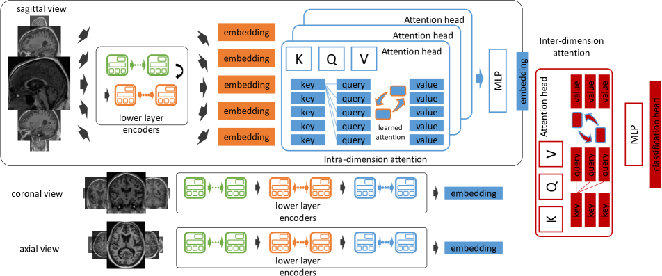
Figure 2: The detailed architecture for our MedTransformer.

3.1 An Overview of Vision Transformer

Vision Transformer(ViT) [12] is becoming more and more popular because of its ability to extract long-range features of an image. It reshapes a 2D image x $\in$ $\mathbb{R}^{H\times W\times C}$ into an embedding sequence $\textbf{x}_{p}$ $\in$ $\mathbb{R}^{N\times(P^{2}\cdot C)}$ with image patch patch $\in$ $\mathbb{R}^{P\times P}$. Because that Transformer uses constant latent vector size D through all of its layers, so ViT flattens the patches and map to D dimensions with a trainable fully connected layer. The output patch embedding is $\textbf{x}_{p}$ $\in$ $\mathbb{R}^{N\times D}$. Then ViT concatenates a learnable $[class]$ token $\textbf{x}_{class}$ $\in$ $\mathbb{R}^{1\times D}$ at the first position of the embedding sequence similar to BERT [11] for classification. At the same time, to better learn the position relationship between different image patches, ViT also directly adds a learnable position embedding $\textbf{E}_{pos}$ $\in$ $\mathbb{R}^{(N+1)\times D}$ into the input sequence for learning the relationship.

$$\textbf{S}_{0} =\textbf{x}_{class}\oplus\textbf{x}_{p}+\textbf{E}_{pos}\quad\quad \textbf{S}\in\mathbb{R}^{(N+1)\times D}$$ (1)

$$\textbf{S}_{l}^{\prime} ={\rm MSA(LN(}\textbf{S}_{l-1}))+\textbf{S}_{l-1} l=1...L$$ (2)

$$\textbf{S}_{l} ={\rm MLP(LN(}\textbf{S}_{l}^{\prime}))+\textbf{S}_{l}^{\prime} l=1...L$$ (3)

out $$={\rm LN(}(\textbf{x}_{class})_{L})$$ (4)

label $$={\rm MLP}(\textbf{out})$$ (5)

The Transformer Encoder has $L$ layers of multiheaded self-attention (MSA) and MLP blocks. At the same time, Layer Norm (LN) and residual connections are applied before and after blocks.

3.2 MedTransformer Architecture

To better utilize the attention ability but avoid the weakness that ViT is highly sensitive to position information, we propose MedTransformer: a pure transformer-based 2D architecture that focuses on multiple slices and multiple views of 3D images. Figure 2 shows the details. MedTransformer mainly consists of 4 blocks:

• Self-Attention Encoders (SAE) across three views

• Dimension-specific Self-Attention Encoders (DS-AE)

• Intra-dimension Cross-Attention Encoders (IntraCAE)

• Inter-dimension Cross-Attention Encoders (InterCAE)

First, we cut the 3D image into multiple slices along different views. To better obtain the complete information of the 3D image, we cut each image along three views: sagittal view, coronal view, and axial view. We use $n$ images from each view as the model input. Then similar to ViT, MedTransformer also uses the image patch and patch embedding method to embed the 2D images into 3 sequences including $3\times n$ slices with guide patch embedding layer $\textbf{x}_{guide}$, then concatenates them together as the input to the transformer encoders (Eq. 6). The guide patch embedding aims to reshape the whole sequence into a sequence of flattened 2D patches that has the same shape as the sequence after the normal patch, which means the guide patch embedding has the input channel with the number $3\times n$. By doing this, we can simply add the global information into each special slice sequence. MedTransformer adds learnable position embedding to $\textbf{S}_{0}$ for the patch embedding sequence. (Eq. 7).

$$\textbf{S}_{0}=[\textbf{x}_{class};\underbrace{\textbf{x}_{p_{1}}+\textbf{x}_{guide};\cdots;\textbf{x}_{p_{n}}+\textbf{x}_{guide}}_{sagittal};$$ (6)

$$\underbrace{\cdots;\textbf{x}_{p_{2n}}+\textbf{x}_{guide}}_{coronal};\underbrace{\cdots;\textbf{x}_{p_{3n}}+\textbf{x}_{guide}}_{axial}]$$

$$\textbf{S}_{0}=\textbf{S}_{0}+\textbf{E}_{pos}\quad\quad\textbf{E}_{pos}\in\mathbb{R}^{(3\cdot n\cdot N+1)\times D}$$ (7)

Second, the lower layer encoders take $\textbf{S}_{0}$ as input and learn the bias attention among multiple slices and multiple views. To be more specific, the shared Self-Attention Encoders (SAE) across three view dimensions are designed to learn not only the attention of the slice itself but also the relationship between all slices. These networks are Siamese networks [21] which share the same weights. Also, we set the $[class]$ token of each slice $\textbf{x}_{class}^{s}=\textbf{x}_{class}$ before training the network.

$$\textbf{S}_{0}^{s}=[\textbf{x}_{class}^{s};\textbf{x}_{p_{s}}]\quad\quad s\in(1,3\cdot n)$$ (8)

$$\textbf{S}_{l}^{s}={\rm SAE(\textbf{S}_{\textit{l-1}}^{\textit{s}})}\quad\quad l=1...L_{\textnormal{SAE}}$$ (9)

The Dimension-specific Self-Attention Encoders (DS-AE) also aim to learn the attention of the slice itself. However, compared with SAE, these encoders only learn the relationship between the slices from the same dimension sequence. So in MedTransformer design, there will be three different encoders, each having the same number of layers $L_{\textnormal{DSAE}}$. In the following equation, t means the three different views.

$$\textbf{S}_{l}^{t\cdot s}={\rm DSAE_{t}}(\textbf{S}_{\textit{l-1}}^{t\cdot s}{\rm)}\quad\quad s\in(1,n),t\in(1,3)$$ (10)

$$l=(L_{\textnormal{SAE}}+1)...(L_{\textnormal{SAE}}+L_{\textnormal{DSAE}})$$

Then the output of DSAE from each view will be the input of Intra-dimension Cross-Attention Encoders (IntraCAE) of each view. Here MedTransformer will apply cross embedding mechanism to the input embeddings. (Details are in section 3.3.) After the IntraCAE, the embeddings will combine the features from different slices of the same view sufficiently. Following the architecture of DSAE, each view-dependent encoder will have $L_{\textnormal{IntraCAE}}$ layers.

$$\textbf{S}_{l}^{t\cdot s}= {\rm IntraCAE_{t}}(\textbf{S}_{\textit{l-1}}^{t\cdot s}{\rm)}\quad\quad s\in(1,n),t\in(1,3)$$ (11)

$$l= (L_{\textnormal{SAE}}+L_{\textnormal{DSAE}}+1)...$$

$$(L_{\textnormal{SAE}}+L_{\textnormal{DSAE}}+L_{\textnormal{IntraCAE}})$$

After combining the features between slices of the same dimension independently, the Inter-dimension Cross-Attention Encoders (InterCAE) are proposed to learn the inter-dimension relationship between different sequences from different views. InterCAE will apply cross embedding mechanism again into the view-dependent embeddings. Here MedTransformer only has one encoder with $L_{\textnormal{InterCAE}}$ layers.

$$\textbf{S}_{l}^{t} ={\rm InterCAE_{t}}(\textbf{S}_{\textit{l-1}}^{t}{\rm)}\quad\quad t\in(1,3)$$ (12)

$$l =(L_{\textnormal{SAE}}+L_{\textnormal{DSAE}}+L_{\textnormal{IntraCAE}}+1)...$$

$$(L_{\textnormal{SAE}}+L_{\textnormal{DSAE}}+L_{\textnormal{IntraCAE}}+L_{\textnormal{InterCAE}})$$

Finally, the $[class]$ tokens of the output from three dimensions will be averaged and sent to Layer Norm and classification MLP head as Eq. 4 and Eq. 5 to get the final diagnosis result: AD or normal.

3.3 Fusion Attention Mechanism

To better combine the information among different slices and different views, we propose a simple but novel cross-attention mechanism. We call this mechanism fusion attention. The fusion attention mechanism tries to add the embeddings together directly. However, different from simply adding them together one by one, it adds the embeddings representing the patches but not the tokens. Please note that the $[class]$ token of each embedding has aggregated the information from one slice in previous encoders, so this operation aims to let the embeddings more focus on themselves when learning attention. At the same time, it can also extract the feature information from other slices or dimensions. Here also takes IntraCAE as an example:

$$\textbf{S}_{l}^{t\cdot s}=\textbf{x}_{class}^{t\cdot s}\oplus(\textbf{x}_{p_{(t-1)\cdot n+1}}+\cdots+\textbf{x}_{p_{t\cdot n}})$$ (13)

$${\rm where}\quad s\in(1,n),t\in(1,3)$$

Let’s consider it using a more mathematical way with the example of two embeddings. The traditional attention mechanism is shown as Eq. 14. After fusing these two embeddings, the K matrix of the first embedding will consist of the K value corresponding to the $[class]$ token from the first embedding, and the K matrix corresponding to fusion embedding. The Q matrix is similar. After the matrix calculation, Eq. 16 greatly fuses the information from two embeddings while keeping some unique information from the special $[class]$ token.

$$H=softmax(\frac{QK^{T}}{\sqrt{d_{k}}})V$$ (14)

$$K_{1}=[K_{class_{1}},K_{1}+K_{2}],Q_{1}=[Q_{class_{1}},Q_{1}+Q_{2}]$$ (15)

$$QK^{T}=\begin{bmatrix}Q_{class_{1}}K_{class_{1}}&(Q_{1}+Q_{2})K_{class_{1}}\\ Q_{class_{1}}(K_{1}+K_{2})&(Q_{1}+Q_{2})(K_{1}+K_{2})\end{bmatrix}$$ (16)

3.4 Morphology Augmentation

After visualizing the AD and normal images, we uncover a crucial insight: the atrophy of the brain mass size between these two kinds of images are significantly different. Based on this finding, we propose morphology augmentation, an augmentation method which can help to expand and reduce the size of the atrophy, causing the improvement of the model in distinguishing the two classes. This augmentation is based on scale erosion and dilation shown in Eq.  17, 18. f is the input image, $b_{N}$ is the erosion or dilation element, (x,y) and (s,t) are the coordinates in f and $b_{N}$ respectively.

$$[f\ominus b_{N}](x,y)=\min\limits_{(s,t)\in b_{N}}\left\{f(x+s,y+t)-b_{N}(s,t)\right\}$$ (17)

$$[f\oplus b_{N}](x,y)=\max\limits_{(s,t)\in b_{N}}\left\{f(x-s,y-t)+b_{N}(s,t)\right\}$$ (18)

The visualization of morphology augmentation is shown in Fig. 3. We do erosion-based morphology augmentation to the Alzheimer’s Disease(AD) image and dilation-based morphology augmentation to the Normal Control(NC) image. The size of the atrophy is increased in AD but decreased in NC. With the morphology augmentation, we can not only augment the AD and NC images but also utilize the MCI data more efficiently. Because the MCI is the prodromal stage of AD, so we can do erosion-based morphology augmentation to the MCI data and classify them as AD, while doing dilation-based morphology augmentation to the MCI data and then classify them as normal data.

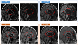
Figure 3: The Alzheimer’s Disease (AD) image, Normal Control (NC) image, and Mild Cognitive Impairment (MCI) image before (left) and after (right) morphology augmentation.

4 Experiments

Model name	ADNI		AIBL	MIRIAD	OASIS
	val acc.	test acc.	test acc.	test acc.	test acc.
MedicalNet-18	0.827	0.793	0.856	0.847	0.793
MedicalNet-18	0.756	0.743	0.820	0.800	0.809
MedicalNet-34	0.571	0.669	0.847	0.782	0.585
MedicalNet-50	0.588	0.471	0.303	0.706	0.317
MedicalNet-101	0.558	0.425	0.320	0.656	0.291
MedicalNet-152	0.564	0.381	0.175	0.662	0.239
MedicalNet-200	0.556	0.361	0.125	0.665	0.220
COVID-ViT	0.506	0.573	0.644	0.338	0.715
Uni4Eye	0.622	0.646	0.697	0.647	0.688
MedTransformer	0.781	0.810	0.863	0.756	0.811

Table 1: Comparison of accuracy various 3D CNN-based and transformer-based models on multi-institutional Alzheimer’s disease dataset.

4.1 Experimental Dataset

To verify the efficiency of our MedTransformer, we use the dataset from the Alzheimer’s Disease Neuroimaging Initiative (ADNI) for the training process. This dataset consists of MRI images of T1-weighted magnetic resonance imaging subjects. There are a total of 3,891 3D MR images in the dataset, including 1,216 normal cases (NC), 1,110 AD cases and 1,565 MCI cases. During the training, 878 normal images, 884 AD images and 1565 MCI images were split into the training set, with 72 normal images and 81 AD images as a validation set, together with 266 normal images and 145 AD images as a testing set.

At the same time, to evaluate the performance of our MedTransformer and other deep learning baseline models, we also consider other datasets as test sets. We mainly acquire them from three other institutions with the ADNI test dataset: Australian Imaging, Biomarker and Lifestyle Flagship Study of Ageing (AIBL), Minimal Interval Resonance Imaging in Alzheimer’s Disease (MIRIAD), and The Open Access Series of Imaging Studies (OASIS). The AIBL dataset contains a total of 481 cases which consist of 363 NC, 50 AD cases and 68 MCI cases. Note that when testing, we drop all the MCI cases. So there are total 413 images with 363 NC and 50 AD in AIBL dataset. The MIRIAD dataset contains a total of 523 cases which consist of 177 NC and 346 AD cases. The OASIS dataset contains a total of 2157 cases which consist of 1692 NC and 465 AD cases. Each of the images for any dataset is a 3D grayscale image, meaning that only has 1 channel as input.

4.2 Implementation Details

We implement consistent data pre-processing techniques to normalize and standardize MR images sourced from a multi-institutional database. We first do data augmentation in the following steps. we have followed closely the recommended protocol from the medical community [51] to process the data. Firstly, we do bias field correction with N4ITK method [44]. Next, we register each image to the MNI space [15, 14] with the ICBM 2009c nonlinear symmetric template by performing a affine registration using the SyN algorithm [2] from ANTs [1]. At the same time, the registered images were further cropped to remove the background to improve the computational efficiency. These operations result in images of size 169 × 208 × 179, with 1 mm isotropic voxels. Intensity rescaling, which was performed based on the minimum and maximum values, denoted as MinMax, was also set to be optional to study its influence on the classification results. Finally, the deep QC system [16] is performed to check the quality of the linearly registered data. The software outputs a probability indicating how accurate the registration is. We excluded the scans with a probability lower than 0.5. Overall, the registration process we perform on the data maps different sets of images into a single coordinate system to prepare the data for our later usage.

We also use the Torchio library [36] to do data augmentation. We only apply this augmentation to the training dataset while keeping the validation and testing dataset unchanged. At the same time, we resize all the MR images with Scipy library [46] into 224$\times$224$\times$224 to better fit the input of our MedTransformer. Finally, we employed the zero-mean unit-variance method to normalize the intensity of all voxels within the images.

For the training dataset, we leverage MCI data more smartly. We do morphology augmentation to the same MCI data, classify the MCI into NC after doing dilation-based augmentation, and classify it into AD after doing erosion-based augmentation. In this way, each MCI is used twice, significantly enlarging the dataset. At the same time, we also do morphology augmentation to AD and NC images randomly, with a probability of 0.5.

After preprocessing the 3D MR images, we cut them into 2D slices along sagittal, coronal and axial views. Then we choose a number of slices in each view and concatenate them into a sequence. We choose 20 equidistant slices on each view and embed them into patch embedding similar to ViT. Here we choose the embed layer from  [43]. Then we use a total of 12 standard transformer attention layers, and 3 layers in each encoder, with 4 heads. At last, because we have three $[class]$ tokens, each representing a special view dimension, we use a classification MLP head, with input feature number 3$\times$256 and output feature number 2, aiming to figure out whether the image is from a disease or not.

We implemented MedTransformer using a Pytorch library [35]. MedTransformer was trained using an AdamW optimizer with learning rate 0.00005. All other parameters are default. At the same time, we also took the advantage of cosine learning rate from [30]. Because this is a binary classification task, we used cross-entropy loss [56]. The training process used five 24G NVIDIA A5000 GPUs. Due to the memory capacity, we use 2 batches on each GPU, meaning a total batch size of 10.

4.3 Evaluation Between Baselines

Our MedTransformer was compared with various baseline models, including 3D CNN-based models: MedicalNet [8] and 3D transformer-based models: COVID-VIT [18], Uni4Eye [4]. There are various versions of MedicalNet, each of which is based on a basic Resnet [24] model, such that MedicalNet-10 is based on Resnet-10 respectively.

In this experiment, we chose a total of 90 slices as input, meaning 30 equidistant slices on each view. Because we found that the central part of the 3D images would be more important and consist of more useful information, we applied the important sampling method in our slice-picking stage. To be more specific, for a 224$\times$224$\times 2$24 image, we pick equidistant slices from $\rm 52^{nd}$ to $\rm 172^{nd}$ on each view.

The quantitative performance is presented in Table 1. We chose the model with the best validation accuracy on ADNI and then tested it on various Alzheimer’s disease datasets. Overall, MedTransformer achieves the best performance on i.i.d testing scenario (ADNI) as well as two of the three out-of-domain testing scenario (AIBL and OASIS). We believe these results show that MedTransformer is not only superior in Alzheimer’s diagnosis in i.i.d setting, but also fairly robust when the testing data is collected from different facilities. For MIRIAD dataset, MedTransformer also achieves a considerable result although not the best-performing one. We conjecture this is due to the disparity of data characteristics between ADNI and MIRIAD. In particular, we notice that MIRIAD has a distinct ratio of AD vs. normal control in the dataset in comparison to others.

4.4 Ablation Study

Slice Number	ADNI		AIBL	MIRIAD	OASIS
	Val acc.	Test acc.	Test acc.	Test acc.	Test acc.
15	0.679	0.690	0.778	0.536	0.781
20	0.638	0.738	0.846	0.402	0.777
45	0.669	0.721	0.797	0.561	0.771
Ours (30)	0.781	0.810	0.863	0.756	0.811

Table 2: Comparison of accuracy between MedTransformer and three variants ablating with different numbers of 2D slices on each axial, coronal, and sagittal dimension in the four datasets.

Layer Number	ADNI		AIBL	MIRIAD	OASIS
	Val acc.	Test acc.	Test acc.	Test acc.	Test acc.
1+1+2+2	0.713	0.776	0.800	0.685	0.793
2+2+1+1	0.708	0.719	0.769	0.674	0.744
4+4+4+4	0.523	0.670	0.814	0.355	0.789
Ours (3+3+3+3)	0.781	0.810	0.863	0.756	0.811

Table 3: Comparison of accuracy between MedTransformer and three variants ablating with different numbers of transformer layers in each encoder in the four datasets.

Cross-Attention Mechanism	ADNI		AIBL	MIRIAD	OASIS
	Val acc.	Test acc.	Test acc.	Test acc.	Test acc.
No Cross-Attension	0.571	0.683	0.838	0.485	0.785
Class Token Cross-Attention	0.656	0.637	0.654	0.710	0.606
Easy Concat Cross-Attention	0.622	0.655	0.719	0.653	0.681
Ours (Fusion Attention)	0.781	0.810	0.863	0.756	0.811

Table 4: Comparison of accuracy between MedTransformer and three variants ablating different cross attention mechanisms in the four datasets.

Models	ADNI		AIBL	MIRIAD	OASIS
	Val acc.	Test acc.	Test acc.	Test acc.	Test acc.
w/o Morphology Augmentation	0.727	0.714	0.731	0.410	0.698
w/o Guide Eembedding	0.75	0.717	0.814	0.602	0.777
w/o Torchio	0.682	0.710	0.796	0.521	0.781
w/o Pretrained Weights	0.644	0.644	0.702	0.714	0.650
w/o Important Sampling	0.544	0.603	0.508	0.531	0.719
MedTransformer	0.781	0.810	0.863	0.756	0.811

Table 5: Comparison of accuracy between MedTransformer and five variants ablating different training augmentation settings in the four datasets.

To evaluate how effective each block is, we compared our MedTransformer with other variants, changing one setting each time. We first compare how different numbers of slices on each dimension will affect the final result. We chose numbers 15, 20, and 45 as comparisons, and our MedTransformer chooses 30 slices on each view dimension. Table 2 shows that fewer slices may not be enough for transformer encoders to extract all the useful information. However, more slices may lead to overfitting problems due to noisy information extracted.

Then we also changed the transformer attention layers of each encoder. ViT uses 12 layers to embed the sequence, so we also tried to cut 12 layers into 4 encoder blocks equally, meaning 3 layers for each encoder block. At the same time, we also investigate into how the number of layers will affect our MedTransformer performance. The results are shown in Table 3, there are four numbers in each variant, each one corresponding to an encoder block. Such as 1+1+2+2 meaning that the shared self-attention encoders, dimension-specific self-attention encoders, intra-dimension cross-attention encoders and inter-dimension cross-attention encoders have 1, 1, 2, 2 transformer attention layer respectively. The result shows that MedTransformer outperforms all the variants on test accuracy in four different datasets, meaning that 3 layers for each block has its superiority.

Table 4 shows how different cross-attention mechanisms will affect the final result. The first variant: No Cross-Attention, meaning that we didn’t apply any cross-attention mechanism in the last two encoder blocks. Class Token Cross-Attention is a variant of Eq. 15. It adds the $[class]$ token embedding up but not the embedding behind the $[class]$ token. For the easy concat cross-attention mechanism, it simply concatenates the embeddings from different slices and view dimensions into a whole large embedding. Our proposed Fusion Attention achieves more than 12% improvements to the ADNI test result while demonstrating superiority on other testing datasets, verifying that fusion attention cannot only fuse the information while keeping the unique information in each embedding.

Table 5 shows other variables in our settings. We delete one important setting in each variant to see the results. MedTransformer outperforms all variant models in all four datasets by 9.03%, 4.3%, 4.2% and 2.8%, respectively. The results show the great capability of different settings in augmenting the model learning ability to classify 3D MRI.

4.5 Visualization Result

We visualize the activated area our model focusing on based on the transformer attention map. Figure 4 shows a NC-related attention map in 3D MRI images from ADNI dataset in axial, sagittal and coronal views. Because our transformer model has 4 special encoders, we visualize the attention result after each encoder.

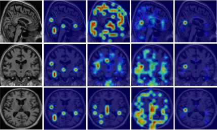
Figure 4: Attention map for Normal Control result.

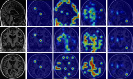
Figure 5: Attention map for Alzheimer’s Disease result.

The attention mostly focuses on the areas that are without the brain mass (thus the atrophic areas of the brain), connecting to the recommended diagnosis procedure of Alzheimer’s from MRI, based on the understanding of its pathology [17].

5 Conclusions

We proposed a 3D medical image classification method, called MedTransformer, that uses various 2D transformer encoder blocks for Alzheimer’s disease diagnosis. The proposed method uses shared self-attention encoders across different view dimensions, dimension-specific self-attention encoders, intra-dimension cross-attention encoders, and inter-dimension cross-attention encoders to extract and combine information from high-dimensional 3D MR images, with novel techniques such as fusion attention mechanism and morphology augmentation. The experiments show that MedTransformer can achieve outstanding performance compared to various 3D image classification networks in multi-institutional test datasets. The visualization results show that MedTransformer can successfully focus on AD-related regions of 3D MRI images, guiding clinical research on Alzheimer’s Disease.

References

- Avants et al. [2008] Brian B Avants, Charles L Epstein, Murray Grossman, and James C Gee. Symmetric diffeomorphic image registration with cross-correlation: evaluating automated labeling of elderly and neurodegenerative brain. Medical image analysis, 12(1):26–41, 2008.
- Avants et al. [2014] Brian B Avants, Nicholas J Tustison, Michael Stauffer, Gang Song, Baohua Wu, and James C Gee. The insight toolkit image registration framework. Frontiers in neuroinformatics, 8:44, 2014.
- Baumgartner et al. [2019] Christian F Baumgartner, Kerem C Tezcan, Krishna Chaitanya, Andreas M Hötker, Urs J Muehlematter, Khoschy Schawkat, Anton S Becker, Olivio Donati, and Ender Konukoglu. Phiseg: Capturing uncertainty in medical image segmentation. In Medical Image Computing and Computer Assisted Intervention–MICCAI 2019: 22nd International Conference, Shenzhen, China, October 13–17, 2019, Proceedings, Part II 22, pages 119–127. Springer, 2019.
- Cai et al. [2022] Zhiyuan Cai, Li Lin, Huaqing He, and Xiaoying Tang. Uni4eye: Unified 2d and 3d self-supervised pre-training via masked image modeling transformer for ophthalmic image classification. In International Conference on Medical Image Computing and Computer-Assisted Intervention, pages 88–98. Springer, 2022.
- Carion et al. [2020] Nicolas Carion, Francisco Massa, Gabriel Synnaeve, Nicolas Usunier, Alexander Kirillov, and Sergey Zagoruyko. End-to-end object detection with transformers. In European conference on computer vision, pages 213–229. Springer, 2020.
- Chen et al. [2021] Chun-Fu Richard Chen, Quanfu Fan, and Rameswar Panda. Crossvit: Cross-attention multi-scale vision transformer for image classification. In Proceedings of the IEEE/CVF international conference on computer vision, pages 357–366, 2021.
- Chen et al. [2019a] Liang Chen, Paul Bentley, Kensaku Mori, Kazunari Misawa, Michitaka Fujiwara, and Daniel Rueckert. Self-supervised learning for medical image analysis using image context restoration. Medical image analysis, 58:101539, 2019a.
- Chen et al. [2019b] Sihong Chen, Kai Ma, and Yefeng Zheng. Med3d: Transfer learning for 3d medical image analysis. arXiv preprint arXiv:1904.00625, 2019b.
- Chen et al. [2022] Xuxin Chen, Ximin Wang, Ke Zhang, Kar-Ming Fung, Theresa C Thai, Kathleen Moore, Robert S Mannel, Hong Liu, Bin Zheng, and Yuchen Qiu. Recent advances and clinical applications of deep learning in medical image analysis. Medical Image Analysis, 79:102444, 2022.
- Despotović et al. [2015] Ivana Despotović, Bart Goossens, Wilfried Philips, et al. Mri segmentation of the human brain: challenges, methods, and applications. Computational and mathematical methods in medicine, 2015, 2015.
- Devlin et al. [2018] Jacob Devlin, Ming-Wei Chang, Kenton Lee, and Kristina Toutanova. Bert: Pre-training of deep bidirectional transformers for language understanding. arXiv preprint arXiv:1810.04805, 2018.
- Dosovitskiy et al. [2020] Alexey Dosovitskiy, Lucas Beyer, Alexander Kolesnikov, Dirk Weissenborn, Xiaohua Zhai, Thomas Unterthiner, Mostafa Dehghani, Matthias Minderer, Georg Heigold, Sylvain Gelly, et al. An image is worth 16x16 words: Transformers for image recognition at scale. arXiv preprint arXiv:2010.11929, 2020.
- Farooq et al. [2017] Ammarah Farooq, SyedMuhammad Anwar, Muhammad Awais, and Saad Rehman. A deep cnn based multi-class classification of alzheimer’s disease using mri. In 2017 IEEE International Conference on Imaging systems and techniques (IST), pages 1–6. IEEE, 2017.
- Fonov et al. [2011] Vladimir Fonov, Alan C Evans, Kelly Botteron, C Robert Almli, Robert C McKinstry, D Louis Collins, Brain Development Cooperative Group, et al. Unbiased average age-appropriate atlases for pediatric studies. Neuroimage, 54(1):313–327, 2011.
- Fonov et al. [2009] Vladimir S Fonov, Alan C Evans, Robert C McKinstry, C Robert Almli, and DL Collins. Unbiased nonlinear average age-appropriate brain templates from birth to adulthood. NeuroImage, 47:S102, 2009.
- Fonov et al. [2018] Vladimir S Fonov, Mahsa Dadar, Prevent-Ad Research Group, and D Louis Collins. Deep learning of quality control for stereotaxic registration of human brain mri. bioRxiv, page 303487, 2018.
- Frisoni et al. [2010] Giovanni B Frisoni, Nick C Fox, Clifford R Jack Jr, Philip Scheltens, and Paul M Thompson. The clinical use of structural mri in alzheimer disease. Nature Reviews Neurology, 6(2):67–77, 2010.
- Gao et al. [2021] Xiaohong Gao, Yu Qian, and Alice Gao. Covid-vit: Classification of covid-19 from ct chest images based on vision transformer models. arXiv preprint arXiv:2107.01682, 2021.
- Guan et al. [2018] Qingji Guan, Yaping Huang, Zhun Zhong, Zhedong Zheng, Liang Zheng, and Yi Yang. Diagnose like a radiologist: Attention guided convolutional neural network for thorax disease classification. arXiv preprint arXiv:1801.09927, 2018.
- Guan et al. [2022] Tianrui Guan, Jun Wang, Shiyi Lan, Rohan Chandra, Zuxuan Wu, Larry Davis, and Dinesh Manocha. M3detr: Multi-representation, multi-scale, mutual-relation 3d object detection with transformers. In Proceedings of the IEEE/CVF winter conference on applications of computer vision, pages 772–782, 2022.
- Guo et al. [2017] Qing Guo, Wei Feng, Ce Zhou, Rui Huang, Liang Wan, and Song Wang. Learning dynamic siamese network for visual object tracking. In Proceedings of the IEEE international conference on computer vision, pages 1763–1771, 2017.
- Hatamizadeh et al. [2021] Ali Hatamizadeh, Vishwesh Nath, Yucheng Tang, Dong Yang, Holger R Roth, and Daguang Xu. Swin unetr: Swin transformers for semantic segmentation of brain tumors in mri images. In International MICCAI Brainlesion Workshop, pages 272–284. Springer, 2021.
- Hatamizadeh et al. [2022] Ali Hatamizadeh, Yucheng Tang, Vishwesh Nath, Dong Yang, Andriy Myronenko, Bennett Landman, Holger R Roth, and Daguang Xu. Unetr: Transformers for 3d medical image segmentation. In Proceedings of the IEEE/CVF winter conference on applications of computer vision, pages 574–584, 2022.
- He et al. [2016] Kaiming He, Xiangyu Zhang, Shaoqing Ren, and Jian Sun. Deep residual learning for image recognition. In Proceedings of the IEEE conference on computer vision and pattern recognition, pages 770–778, 2016.
- Henschel et al. [2020] Leonie Henschel, Sailesh Conjeti, Santiago Estrada, Kersten Diers, Bruce Fischl, and Martin Reuter. Fastsurfer-a fast and accurate deep learning based neuroimaging pipeline. NeuroImage, 219:117012, 2020.
- Iaccarino et al. [2021] Leonardo Iaccarino, Renaud La Joie, Lauren Edwards, Amelia Strom, Daniel R Schonhaut, Rik Ossenkoppele, Julie Pham, Taylor Mellinger, Mustafa Janabi, Suzanne L Baker, et al. Spatial relationships between molecular pathology and neurodegeneration in the alzheimer’s disease continuum. Cerebral Cortex, 31(1):1–14, 2021.
- Jang and Hwang [2022] Jinseong Jang and Dosik Hwang. M3t: three-dimensional medical image classifier using multi-plane and multi-slice transformer. In Proceedings of the IEEE/CVF conference on computer vision and pattern recognition, pages 20718–20729, 2022.
- Jo et al. [2019] Taeho Jo, Kwangsik Nho, and Andrew J Saykin. Deep learning in alzheimer’s disease: diagnostic classification and prognostic prediction using neuroimaging data. Frontiers in aging neuroscience, 11:220, 2019.
- Liu et al. [2021] Ze Liu, Yutong Lin, Yue Cao, Han Hu, Yixuan Wei, Zheng Zhang, Stephen Lin, and Baining Guo. Swin transformer: Hierarchical vision transformer using shifted windows. In Proceedings of the IEEE/CVF international conference on computer vision, pages 10012–10022, 2021.
- Loshchilov and Hutter [2016] Ilya Loshchilov and Frank Hutter. Sgdr: Stochastic gradient descent with warm restarts. arXiv preprint arXiv:1608.03983, 2016.
- Luo et al. [2016] Wenjie Luo, Yujia Li, Raquel Urtasun, and Richard Zemel. Understanding the effective receptive field in deep convolutional neural networks. Advances in neural information processing systems, 29, 2016.
- Misra et al. [2021] Ishan Misra, Rohit Girdhar, and Armand Joulin. An end-to-end transformer model for 3d object detection. In Proceedings of the IEEE/CVF International Conference on Computer Vision, pages 2906–2917, 2021.
- Oktay et al. [2018] Ozan Oktay, Jo Schlemper, Loic Le Folgoc, Matthew Lee, Mattias Heinrich, Kazunari Misawa, Kensaku Mori, Steven McDonagh, Nils Y Hammerla, Bernhard Kainz, et al. Attention u-net: Learning where to look for the pancreas. arXiv preprint arXiv:1804.03999, 2018.
- Pan et al. [2021] Xuran Pan, Zhuofan Xia, Shiji Song, Li Erran Li, and Gao Huang. 3d object detection with pointformer. In Proceedings of the IEEE/CVF Conference on Computer Vision and Pattern Recognition, pages 7463–7472, 2021.
- Paszke et al. [2019] Adam Paszke, Sam Gross, Francisco Massa, Adam Lerer, James Bradbury, Gregory Chanan, Trevor Killeen, Zeming Lin, Natalia Gimelshein, Luca Antiga, et al. Pytorch: An imperative style, high-performance deep learning library. Advances in neural information processing systems, 32, 2019.
- Pérez-García et al. [2021] Fernando Pérez-García, Rachel Sparks, and Sébastien Ourselin. Torchio: a python library for efficient loading, preprocessing, augmentation and patch-based sampling of medical images in deep learning. Computer Methods and Programs in Biomedicine, 208:106236, 2021.
- Qi et al. [2017] Charles R Qi, Hao Su, Kaichun Mo, and Leonidas J Guibas. Pointnet: Deep learning on point sets for 3d classification and segmentation. In Proceedings of the IEEE conference on computer vision and pattern recognition, pages 652–660, 2017.
- Salehi et al. [2020] Ahmad Waleed Salehi, Preety Baglat, Brij Bhushan Sharma, Gaurav Gupta, and Ankita Upadhya. A cnn model: earlier diagnosis and classification of alzheimer disease using mri. In 2020 International Conference on Smart Electronics and Communication (ICOSEC), pages 156–161. IEEE, 2020.
- Setio et al. [2017] Arnaud Arindra Adiyoso Setio, Alberto Traverso, Thomas De Bel, Moira SN Berens, Cas Van Den Bogaard, Piergiorgio Cerello, Hao Chen, Qi Dou, Maria Evelina Fantacci, Bram Geurts, et al. Validation, comparison, and combination of algorithms for automatic detection of pulmonary nodules in computed tomography images: the luna16 challenge. Medical image analysis, 42:1–13, 2017.
- Silva et al. [2019] Iago RR Silva, Gabriela SL Silva, Rodrigo G de Souza, Wellington P dos Santos, and Roberta A de A Fagundes. Model based on deep feature extraction for diagnosis of alzheimer’s disease. In 2019 international joint conference on neural networks (IJCNN), pages 1–7. IEEE, 2019.
- Simpson et al. [2019] Amber L Simpson, Michela Antonelli, Spyridon Bakas, Michel Bilello, Keyvan Farahani, Bram Van Ginneken, Annette Kopp-Schneider, Bennett A Landman, Geert Litjens, Bjoern Menze, et al. A large annotated medical image dataset for the development and evaluation of segmentation algorithms. arXiv preprint arXiv:1902.09063, 2019.
- Tajbakhsh et al. [2020] Nima Tajbakhsh, Laura Jeyaseelan, Qian Li, Jeffrey N Chiang, Zhihao Wu, and Xiaowei Ding. Embracing imperfect datasets: A review of deep learning solutions for medical image segmentation. Medical Image Analysis, 63:101693, 2020.
- Touvron et al. [2022] Hugo Touvron, Matthieu Cord, Alaaeldin El-Nouby, Jakob Verbeek, and Hervé Jégou. Three things everyone should know about vision transformers. In European Conference on Computer Vision, pages 497–515. Springer, 2022.
- Tustison et al. [2010] Nicholas J Tustison, Brian B Avants, Philip A Cook, Yuanjie Zheng, Alexander Egan, Paul A Yushkevich, and James C Gee. N4itk: improved n3 bias correction. IEEE transactions on medical imaging, 29(6):1310–1320, 2010.
- Vaswani et al. [2017] Ashish Vaswani, Noam Shazeer, Niki Parmar, Jakob Uszkoreit, Llion Jones, Aidan N Gomez, Łukasz Kaiser, and Illia Polosukhin. Attention is all you need. Advances in neural information processing systems, 30, 2017.
- Virtanen et al. [2020] Pauli Virtanen, Ralf Gommers, Travis E Oliphant, Matt Haberland, Tyler Reddy, David Cournapeau, Evgeni Burovski, Pearu Peterson, Warren Weckesser, Jonathan Bright, et al. Scipy 1.0: fundamental algorithms for scientific computing in python. Nature methods, 17(3):261–272, 2020.
- Wang et al. [2020] Huiyu Wang, Yukun Zhu, Bradley Green, Hartwig Adam, Alan Yuille, and Liang-Chieh Chen. Axial-deeplab: Stand-alone axial-attention for panoptic segmentation. In European conference on computer vision, pages 108–126. Springer, 2020.
- Wang et al. [2019] Yue Wang, Yongbin Sun, Ziwei Liu, Sanjay E Sarma, Michael M Bronstein, and Justin M Solomon. Dynamic graph cnn for learning on point clouds. ACM Transactions on Graphics (tog), 38(5):1–12, 2019.
- Wang et al. [2021] Yuqing Wang, Zhaoliang Xu, Xinlong Wang, Chunhua Shen, Baoshan Cheng, Hao Shen, and Huaxia Xia. End-to-end video instance segmentation with transformers. In Proceedings of the IEEE/CVF conference on computer vision and pattern recognition, pages 8741–8750, 2021.
- Wang et al. [2023] Yifeng Wang, Zhi Tu, Yiwen Xiang, Shiyuan Zhou, Xiyuan Chen, Bingxuan Li, and Tianyi Zhang. Rapid image labeling via neuro-symbolic learning. arXiv preprint arXiv:2306.10490, 2023.
- Wen et al. [2020] Junhao Wen, Elina Thibeau-Sutre, Mauricio Diaz-Melo, Jorge Samper-González, Alexandre Routier, Simona Bottani, Didier Dormont, Stanley Durrleman, Ninon Burgos, Olivier Colliot, et al. Convolutional neural networks for classification of alzheimer’s disease: Overview and reproducible evaluation. Medical image analysis, 63:101694, 2020.
- Yan et al. [2019] Ke Yan, Yifan Peng, Veit Sandfort, Mohammadhadi Bagheri, Zhiyong Lu, and Ronald M Summers. Holistic and comprehensive annotation of clinically significant findings on diverse ct images: learning from radiology reports and label ontology. In Proceedings of the IEEE/CVF Conference on Computer Vision and Pattern Recognition, pages 8523–8532, 2019.
- Yu et al. [2021] Jianhui Yu, Chaoyi Zhang, Heng Wang, Dingxin Zhang, Yang Song, Tiange Xiang, Dongnan Liu, and Weidong Cai. 3d medical point transformer: Introducing convolution to attention networks for medical point cloud analysis. arXiv preprint arXiv:2112.04863, 2021.
- Yu et al. [2019] Lequan Yu, Shujun Wang, Xiaomeng Li, Chi-Wing Fu, and Pheng-Ann Heng. Uncertainty-aware self-ensembling model for semi-supervised 3d left atrium segmentation. In Medical Image Computing and Computer Assisted Intervention–MICCAI 2019: 22nd International Conference, Shenzhen, China, October 13–17, 2019, Proceedings, Part II 22, pages 605–613. Springer, 2019.
- Yu et al. [2022] Xumin Yu, Lulu Tang, Yongming Rao, Tiejun Huang, Jie Zhou, and Jiwen Lu. Point-bert: Pre-training 3d point cloud transformers with masked point modeling. In Proceedings of the IEEE/CVF Conference on Computer Vision and Pattern Recognition, pages 19313–19322, 2022.
- Zhang and Sabuncu [2018] Zhilu Zhang and Mert Sabuncu. Generalized cross entropy loss for training deep neural networks with noisy labels. Advances in neural information processing systems, 31, 2018.
- Zhu et al. [2023] Haoran Zhu, Boyuan Chen, and Carter Yang. Understanding why vit trains badly on small datasets: An intuitive perspective. arXiv preprint arXiv:2302.03751, 2023.