A Fully Bayesian Approach for Comprehensive Mapping of Magnitude and Phase Brain Activation in Complex-Valued fMRI Data

Abstract

Functional magnetic resonance imaging (fMRI) plays a crucial role in neuroimaging, enabling the exploration of brain activity through complex-valued signals. These signals, composed of magnitude and phase, offer a rich source of information for understanding brain functions. Traditional fMRI analyses have largely focused on magnitude information, often overlooking the potential insights offered by phase data. In this paper, we propose a novel fully Bayesian model designed for analyzing single-subject complex-valued fMRI (cv-fMRI) data. Our model, which we refer to as the CV-M&P model, is distinctive in its comprehensive utilization of both magnitude and phase information in fMRI signals, allowing for independent prediction of different types of activation maps. We incorporate Gaussian Markov random fields (GMRFs) to capture spatial correlations within the data, and employ image partitioning and parallel computation to enhance computational efficiency. Our model is rigorously tested through simulation studies, and then applied to a real dataset from a unilateral finger-tapping experiment. The results demonstrate the model’s effectiveness in accurately identifying brain regions activated in response to specific tasks, distinguishing between magnitude and phase activation.

Key words and phrases: Gibbs sampling, parallel computation, phase analysis, Rowe–Logan, spike and slab prior, variable selection.

1 Introduction

Magnetic resonance imaging (MRI) is a non-invasive imaging technique that has revolutionized the field of medical diagnostics and research, particularly in the realm of neuroimaging. Functional magnetic resonance imaging (fMRI) is a subtype of MRI specifically optimized for higher temporal resolution. While conventional MRI captures static anatomical details, fMRI extends the utility by enabling the examination of metabolic functions over time. It has become indispensable in a variety of applications ranging from diagnosis of pathological conditions to the investigation of complex physiological processes in the human brain.

FMRI inherently generates complex-valued signals characterized by real and imaginary components, and further summarized as magnitude and phase. This complex structure arises from the forward and inverse Fourier transformations executed in the data collection process, which are affected by phase imperfections (Brown et al., 2014). These signals may exhibit changes in magnitude, phase, or both over time in response to a stimulus, as shown in Figure 1.

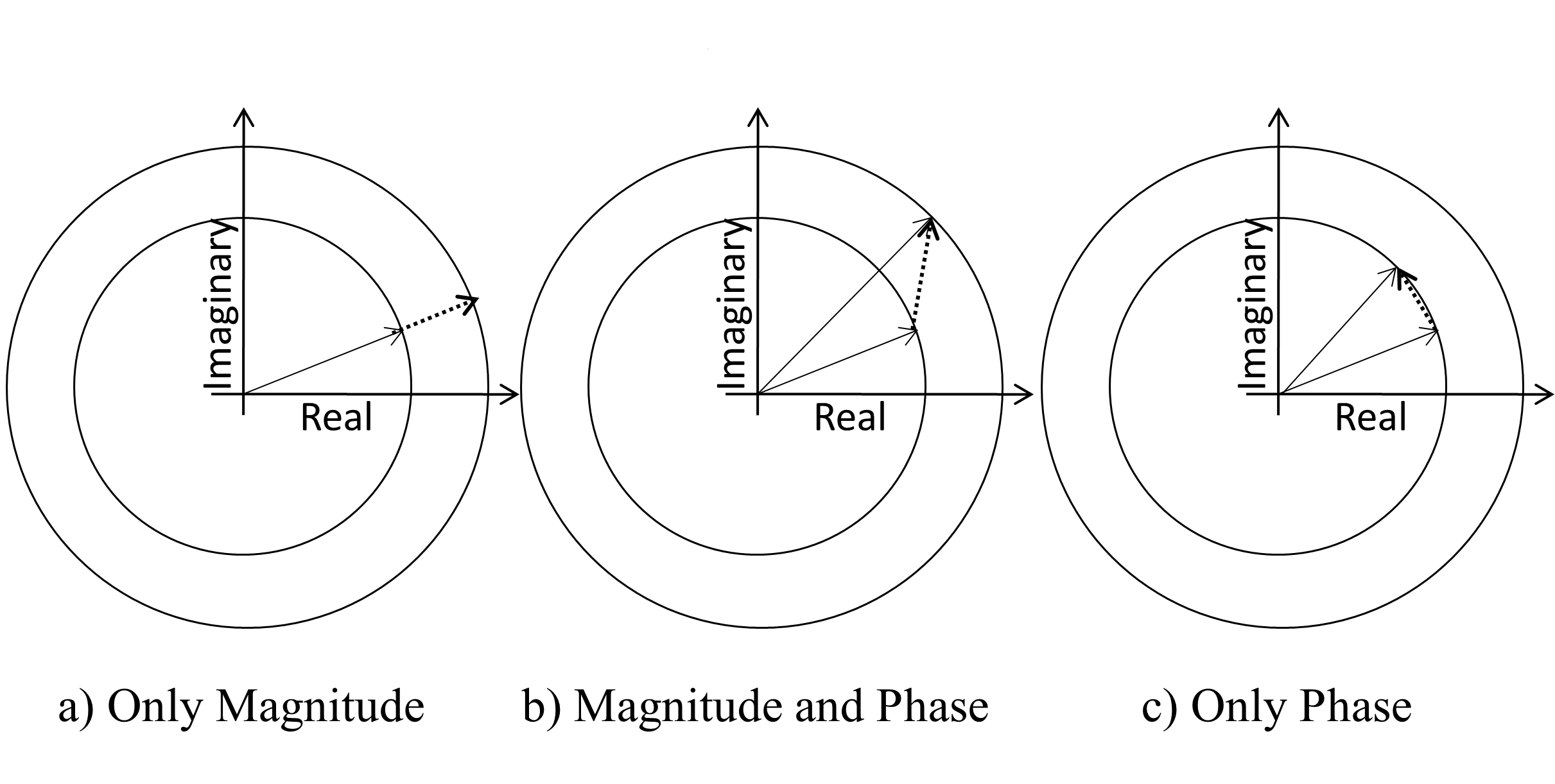
Figure 1: Illustration of potential changes in complex-valued fMRI time series (Rowe, 2019).

The magnitude changes in complex-valued fMRI (cv-fMRI) are fundamentally driven by the blood-oxygenation-level-dependent (BOLD) effect, which operates through a cascade of hemodynamic responses. Neuronal activity leads to increased demand of oxygen, so the freshly oxygenated blood fluxes into the active region and displaces deoxygenated blood, leading to an overall increase in the oxygenation level of the blood in that region. These changes in blood oxygenation cause a change in BOLD signal and magnetic susceptibility, affecting the magnitude of MR signal. Thus, the BOLD effect can be considered an indirect measure of neuronal activity, mediated through vascular changes (Boynton et al., 1996; Logothetis, 2008).

On the other hand, phase changes are influenced not only by the BOLD effect but also by the electrical neuronal activities directly. These activities generate moving charges, and therefore create magnetic field which changes the phase of MRI signal. For this reason, the phase changes are able to reveal the aspects of neuronal activity or other phenomena that might be undetected by magnitude-based analyses (Petridou et al., 2006). By accurately modeling these phase changes, researchers can gain insights into the more direct effects of neuronal activity on the MRI signal, potentially leading to more precise and informative interpretations of fMRI data (Feng et al., 2009). This is especially crucial in understanding complex brain functions and improving the accuracy of fMRI in research and clinical applications.

Traditionally, fMRI studies that aim to map brain activity have predominantly focused on analyzing only the magnitude of these MR signals (Friston et al., 1994; Lindquist, 2008). The phase components are frequently disregarded during the preprocessing steps. The magnitude-only analytical framework has its limitations. The first major limitation is that the omission of phase data results in the underutilization of valuable information that could be pertinent to understanding neurophysiological mechanisms. The second limitation, particularly relevant in studies that employ linear modeling (Friston et al., 1994; Lindquist, 2008), concerns the statistical assumptions made during the identification of active voxels (volumetric pixels in the imaging data). In such analyses, the expected BOLD response is usually modeled by the convolution of a “boxcar” binary stimulus function with either a gamma or double-gamma hemodynamic response function (HRF), then a voxel is identified as “active” if the magnitude of its complex-valued fMRI signal significantly varies with the expected BOLD response. This practice assumes that the error terms in the models are normally distributed. However, while the original real and imaginary components may follow a normal distribution, the magnitude actually adheres to a Ricean distribution that approximates a normal distribution only when the signal-to-noise ratios (SNRs) are sufficiently large (Rice, 1944; Gudbjartsson and Patz, 1995). Given that large SNRs are not universally guaranteed in fMRI studies, this statistical assumption becomes less reliable and exacerbates the limitation, consequently diminishing the power and reliability of the analysis.

In contrast, emerging research utilizing cv-fMRI data offers a more nuanced and comprehensive approach. By incorporating both the magnitude and phase of the MR signals (Rowe and Logan, 2004, 2005; Rowe, 2005b, a; Rowe et al., 2007; Rowe, 2009; Adrian et al., 2018), or modeling real and imaginary components that both contain magnitude and phase information (Lee et al., 2007; Yu et al., 2018), cv-fMRI studies pave the way for the development of more robust and statistically powerful models. These models are better to handle variations in SNR and can fully exploit the available data, thereby offering potentially deeper and more accurate insights into task-related neuronal activity.

To accurately determine task-related brain activation maps from fMRI signals, fully Bayesian approaches have garnered attention due to their capacity to effectively model both spatial and temporal correlations. However, existing implementations of fully Bayesian methods in fMRI analysis have demonstrated notable shortcomings. For instance, certain studies have applied the fully Bayesian approach only to magnitude data (Woolrich et al., 2004; Musgrove et al., 2016), leading to underutilization of available data and flawed statistical assumptions as previously discussed. Additionally, others have employed fully Bayesian methods on cv-fMRI data, yet relied on a Cartesian model (Yu et al., 2023; Wang et al., 2023), which is limited to identifying active voxels without providing specific insights into the type of activation, be it in terms of magnitude, phase, or a combination of both.

In this paper, we propose a novel fully Bayesian model for mapping brain activity using single-subject cv-fMRI time series. Our model is designed to determine which voxels exhibit significant fMRI signal changes in response to a particular task, specifying the type and strength of these changes. This proposed Bayesian approach for fMRI data analysis is distinctive in its comprehensive utilization of both the real and imaginary components of fMRI data. It is capable of independently predicting different types of activation maps, in terms of magnitude, or phase, or both, capturing spatial correlations, and ensuring computational efficiency.

To achieve this, our approach incorporates Gaussian Markov random fields (GMRFs; Rue and Held, 2005) to effectively capture spatial associations present in cv-fMRI data. Moreover, we enhance computational efficiency by employing image partitioning and parallel computation strategies in our Markov chain Monte Carlo (MCMC; Gelfand and Smith, 1990) algorithms.

The paper is structured as follows: Section 2 introduces our proposed model, its parameters, and brain parcellation strategy. Section 3 presents simulation studies and compares our approach with existing methods. In Section 4, we apply our model to a real finger-tapping experiment dataset. Section 5 summarizes our findings and suggests future research directions.

2 Model

In this section, we present our model designed for mapping brain activity using cv-fMRI data. Additionally, we introduce the brain parcellation strategy, which facilitates the parallel computation. Following this, we detail the implementation of a GMRF prior that effectively captures the spatial correlations inherent within the fMRI data. Finally, we describe an MCMC algorithm for approximating the posterior distribution of the parameters of interest.

2.1 Model Formulation

The polar model of Rowe (2005b) has gained significant attention for modeling complex-valued fMRI data. Originating from the initial formulation with dynamic magnitude and constant phase (Rowe and Logan, 2004), the model has undergone several iterations (Rowe and Logan, 2005; Rowe, 2005a) to arrive at its current version to model both dynamic magnitude and dynamic phase. For a certain voxel $v$ (where $v=1,\ldots,V$) at time $t$ (where $t=1,\ldots,T$), its real and imaginary parts of complex-valued fMRI signal, $y_{v,Rt}$ and $y_{v,It}$, can be modeled as:

$$\begin{pmatrix}y_{v,Rt}\\ y_{v,It}\end{pmatrix}=\begin{pmatrix}\rho_{v,t}\cos{\theta_{v,t}}\\ \rho_{v,t}\sin{\theta_{v,t}}\end{pmatrix}+\begin{pmatrix}\varepsilon_{v,Rt}\\ \varepsilon_{v,It}\end{pmatrix},\quad\begin{pmatrix}\varepsilon_{v,Rt}\\ \varepsilon_{v,It}\end{pmatrix}\sim\mathcal{N}(\mathbf{0},\sigma_{v}^{2}\mathbf{I}_{2}),$$ (1)

where $\rho_{v,t}$ and $\theta_{v,t}$ are temporally varying magnitude and phase given by:

$$\begin{split}\rho_{v,t}&=\beta_{v,0}+x_{t}\beta_{v,1},\\ \theta_{v,t}&=\gamma_{v,0}+u_{t}\gamma_{v,1},\\ \end{split}$$ (2)

where $x_{t}$ and $u_{t}$ are the expected BOLD response and neuronal electromagnetic signal, respectively, at time $t$. Thus, for all time points:

$$\mathbf{y}_{v}=\begin{pmatrix}\mathbf{A}_{R}(\boldsymbol{\gamma}_{v})\\ \mathbf{A}_{I}(\boldsymbol{\gamma}_{v})\end{pmatrix}\mathbf{X}\boldsymbol{\beta}_{v}+\boldsymbol{\varepsilon}_{v},\quad\boldsymbol{\varepsilon}_{v}\sim\mathcal{N}(\mathbf{0},\sigma_{v}^{2}\mathbf{I}_{2T}),$$ (3)

where $\mathbf{y}_{v}=\left[(\mathbf{y}_{v,R})^{\prime},(\mathbf{y}_{v,I})^{\prime}\right]^{\prime}\in\mathbb{R}^{2T}$ stacks real and imaginary components of cv-fMRI signal, and $\mathbf{X}=[\mathbf{1},\mathbf{x}]\in\mathbb{R}^{T\times 2}$ is the design matrix for the magnitude composed of ones and expected BOLD response $\mathbf{x}$. The matrices $\mathbf{A}_{R}(\boldsymbol{\gamma}_{v}),\mathbf{A}_{I}(\boldsymbol{\gamma}_{v})\in\mathbb{R}^{T\times T}$ are diagonal as:

$$\begin{split}\mathbf{A}_{R}(\boldsymbol{\gamma}_{v})&=\begin{pmatrix}\cos(\gamma_{v,0}+u_{1}\gamma_{v,1})&0&\cdots&0\\ 0&\cos(\gamma_{v,0}+u_{2}\gamma_{v,1})&\cdots&0\\ \vdots&\vdots&\ddots&\vdots\\ 0&0&\cdots&\cos(\gamma_{v,0}+u_{t}\gamma_{v,1})\end{pmatrix},\\ \mathbf{A}_{I}(\boldsymbol{\gamma}_{v})&=\begin{pmatrix}\sin(\gamma_{v,0}+u_{1}\gamma_{v,1})&0&\cdots&0\\ 0&\sin(\gamma_{v,0}+u_{2}\gamma_{v,1})&\cdots&0\\ \vdots&\vdots&\ddots&\vdots\\ 0&0&\cdots&\sin(\gamma_{v,0}+u_{t}\gamma_{v,1})\end{pmatrix},\end{split}$$ (4)

with a more compact form:

$$\mathbf{A}_{R}(\boldsymbol{\gamma}_{v})=\text{diag}\left[\cos{\left(\mathbf{U}\boldsymbol{\gamma}_{v}\right)}\right],\quad\mathbf{A}_{I}(\boldsymbol{\gamma}_{v})=\text{diag}\left[\sin{\left(\mathbf{U}\boldsymbol{\gamma}_{v}\right)}\right],\\$$ (5)

where $\mathbf{U}=[\mathbf{1},\mathbf{u}]\in\mathbb{R}^{T\times 2}$ is the design matrix for the phase composed of ones and neuronal electromagnetic signal $\mathbf{u}$. Therefore, $\boldsymbol{\beta}_{v}=\left[\beta_{v,0},\beta_{v,1}\right]^{\prime}\in\mathbb{R}^{2}$ and $\boldsymbol{\gamma}_{v}=\left[\gamma_{v,0},\gamma_{v,1}\right]^{\prime}\in\mathbb{R}^{2}$ are magnitude- and phase-related regression coefficients, respectively. The voxel-specific error term $\boldsymbol{\varepsilon}_{v}$ follows a multivariate normal distribution with the variance-covariance matrix $\sigma_{v}^{2}\mathbf{I}_{2T}$, and a Jeffreys prior can be assigned to $\sigma_{v}^{2}$ as $p(\sigma_{v}^{2})\propto 1/\sigma_{v}^{2}$.

2.2 Brain Parcellation and Spatial Priors

Spatial correlations are a notable characteristic in fMRI signal data. Given that voxels represent an artificial segmentation of the brain’s structure, they frequently display behaviors that are closely aligned with adjacent voxels (Rowe et al., 2009; Nenckaa et al., 2009; Karaman et al., 2014; Rowe, 2019). To effectively model these spatial dependencies, it is beneficial to incorporate spatial structuring in the priors of $\boldsymbol{\gamma}_{v}$ and $\boldsymbol{\beta}_{v}$ or in the hyperparameters of these priors. Moreover, a strategy of brain parcellation is applied to facilitate the parallel computation.

2.2.1 Brain parcellation

In the study by Musgrove et al. (2016), a technique for brain parcellation was introduced, focusing on the identification of active voxels within individual parcels before integrating these findings into a comprehensive map of brain activity. This approach involves dividing brain images into parcels, each containing around 500 voxels. By processing each parcel independently using an identical model and method, the technique allowed for parallel computation, enhancing computational efficiency. Similarly, Wang et al. (2023) adopted a comparable approach but differed in their strategy of dividing the brain into parcels of roughly equal geometric size. Both studies demonstrated that this parcellation strategy effectively minimizes edge effects, ensuring that the classification of border voxels in each parcel remains largely unaffected. Following the methodology of Wang et al. (2023), we partitioned two- or three-dimensional fMRI images into a set number, $G$, of parcels, each of approximately equal geometric size. The choice of $G$ is based on empirical judgment, and as indicated by both Musgrove et al. (2016) and Wang et al. (2023), variations within a reasonable range of $G$ do not significantly impact the results.

2.2.2 Prior distributions of $\boldsymbol{\beta}_{v}$ and $\boldsymbol{\gamma}_{v}$

For each parcel $g$ (where $g=1,\ldots,G$) encompassing $V_{g}$ voxels, we classify a voxel $v$ (where $v=1,\ldots,V_{g}$) based on its activity. Specifically, a voxel is classified magnitude-active if $\beta_{v,1}\neq 0$, and phase-active if $\gamma_{v,1}\neq 0$. Adhering to the spike-and-slab prior (Mitchell and Beauchamp, 1988), the model is expressed as follows:

$$\begin{split}\boldsymbol{\beta}_{v}\mid\lambda_{v},\tau_{g}^{2}&\sim\lambda_{v}\mathcal{N}_{2}\left(\mathbf{0},\tau_{g}^{2}\mathbf{I}\right)+(1-\lambda_{v})\mathcal{N}_{2}\left(\mathbf{0},\begin{pmatrix}\tau_{g}^{2}&0\\ 0&0\end{pmatrix}\right),\\ \boldsymbol{\gamma}_{v}\mid\omega_{v},\xi_{b}^{2}&\sim\omega_{v}\mathcal{N}_{2}\left(\mathbf{0},\xi_{g}^{2}\mathbf{I}\right)+(1-\omega_{v})\mathcal{N}_{2}\left(\mathbf{0},\begin{pmatrix}\xi_{g}^{2}&0\\ 0&0\end{pmatrix}\right).\end{split}$$ (6)

In this formulation, $\lambda_{v},\omega_{v}\in\{0,1\}$ indicate the status of voxel $v$: $\lambda_{v}=1$ for a magnitude-active voxel and $\omega_{v}=1$ for a phase-active voxel, with 0 indicating inactivity in respective domains. The parameters $\tau_{g}^{2}$ and $\xi_{g}^{2}$ represent parcel-specific variances. These variances are constant for all voxels within a particular parcel but may vary across different parcels, and are assigned a Jeffreys prior, that is, $p(\tau_{g}^{2})\propto 1/\tau_{g}^{2}$ and $p(\xi_{g}^{2})\propto 1/\xi_{g}^{2}$, for $g=1,\ldots,G$. The prior distributions can be succinctly represented as:

$$\begin{split}\boldsymbol{\beta}_{v}\mid\lambda_{v},\tau_{g}^{2}&\sim\mathcal{N}_{2}\left(\mathbf{0},\tau_{g}^{2}\mathbf{\Lambda}_{v}\right),\quad\text{where }\mathbf{\Lambda}_{v}=\begin{pmatrix}1&0\\ 0&\lambda_{v}\end{pmatrix},\\ \boldsymbol{\gamma}_{v}\mid\omega_{v},\xi_{g}^{2}&\sim\mathcal{N}_{2}\left(\mathbf{0},\xi_{g}^{2}\mathbf{\Omega}_{v}\right),\quad\text{where }\mathbf{\Omega}_{v}=\begin{pmatrix}1&0\\ 0&\omega_{v}\end{pmatrix}.\end{split}$$ (7)

2.2.3 Spatial prior on $\lambda_{v}$ and $\omega_{v}$

To capture both spatial dependencies and the sparsity of active voxels in brain imaging, we implement a prior distribution for $\lambda_{v}$ and $\omega_{v}$. This approach is rooted in the hypothesis that voxels are more likely to mirror the activity (active/inactive) of their neighboring voxels (Friston et al., 1994; Smith and Fahrmeir, 2007), and there should be only a few active voxels across the entire brain from a simple task experiment (Rao et al., 1996; Epstein and Kanwisher, 1998). We employ the sparse spatial generalized linear mixed model (sSGLMM) prior, formulated by Reich et al. (2006), and later adopted by Hughes and Haran (2013); Musgrove et al. (2016); Wang et al. (2023). For voxel $v$ (where $v=1,...,V_{g}$) within parcel $g$ (where $g=1,...,G$), from the perspective of the magnitude, we suppose that:

$$\begin{split}\lambda_{v}\mid\eta_{\lambda,v}&\stackrel{{\scriptstyle iid}}{{\sim}}{\mathcal{B}}ern\left\{\mathbf{\Phi}(\psi_{\lambda}+\eta_{\lambda,v})\right\},\\ \eta_{\lambda,v}\mid\boldsymbol{\delta}_{\lambda,g}&\sim\mathcal{N}_{1}\left(\mathbf{m}_{v}^{\prime}\boldsymbol{\delta}_{\lambda,g},1\right),\\ \boldsymbol{\delta}_{\lambda,g}\mid\kappa_{\lambda,g}&\sim\mathcal{N}_{q}\left\{\mathbf{0},(\kappa_{\lambda,g}\mathbf{M}_{g}{{}^{\prime}}\mathbf{Q}_{g}\mathbf{M}_{g})^{-1}\right\},\\ \kappa_{\lambda,g}&\sim{\mathcal{G}}amma\left(a_{\kappa},b_{\kappa}\right).\end{split}$$ (8)

From the perspective of the phase:

$$\begin{split}\omega_{v}\mid\eta_{\omega,v}&\stackrel{{\scriptstyle iid}}{{\sim}}{\mathcal{B}}ern\left\{\mathbf{\Phi}(\psi_{\omega}+\eta_{\omega,v})\right\},\\ \eta_{\omega,v}\mid\boldsymbol{\delta}_{\omega,g}&\sim\mathcal{N}_{1}\left(\mathbf{m}_{v}^{\prime}\boldsymbol{\delta}_{\omega,g},1\right),\\ \boldsymbol{\delta}_{\omega,g}\mid\kappa_{\omega,g}&\sim\mathcal{N}_{q}\left\{\mathbf{0},(\kappa_{\omega,g}\mathbf{M}_{g}{{}^{\prime}}\mathbf{Q}_{g}\mathbf{M}_{g})^{-1}\right\},\\ \kappa_{\omega,g}&\sim{\mathcal{G}}amma\left(a_{\kappa},b_{\kappa}\right).\end{split}$$ (9)

In this sSGLMM prior, $\mathbf{\Phi}(\cdot)$ represents the cumulative distribution function (CDF) of the standard normal distribution. The terms $\psi_{\lambda},\psi_{\omega}\in\mathbb{R}$ are fixed tuning parameters. The terms $\eta_{\lambda,v},\eta_{\omega,v}\in\mathbb{R}$ are auxiliary parameters for the probit link functions. Spatial dependencies are modeled through constructs derived from the adjacency matrix $\mathbf{A}_{g}$ of parcel $g$. This matrix, $\mathbf{A}_{g}\in\{0,1\}^{V_{g}\times V_{g}}$, specifies neighborhood relations among voxels, with $\mathbf{A}_{g,uv}=1$ indicating neighboring voxels $u$ and $v$ (based on user-defined criteria, typically voxels sharing an edge or a corner), and 0 otherwise. The matrix $\mathbf{M}_{g}\in\mathbb{R}^{V_{g}\times q}$ is composed of the first $q$ principal eigenvectors of $\mathbf{A}_{g}$. The row vector $\mathbf{m}_{v}^{\prime}\in\mathbb{R}^{1\times{q}}$ is the $v^{\text{th}}$ row of $\mathbf{M}_{g}$, which is called “synthetic spatial predictors” (Hughes and Haran, 2013). The matrix $\mathbf{Q}_{g}\in\mathbb{R}^{{V_{g}}\times{V_{g}}}$ is the graph Laplacian, that is, $\mathbf{Q}_{g}=\text{diag}(\mathbf{A}_{g}{\mathbf{1}}_{V_{g}})-\mathbf{A}_{g}$. The vectors $\boldsymbol{\delta}_{\lambda,g},\boldsymbol{\delta}_{\omega,g}\in\mathbb{R}^{q\times 1}$ are spatial random effects, and $\kappa_{\lambda,g},\kappa_{\omega,g}\in\mathbb{R}$ are spatial smoothing parameters.

This sSGLMM prior captures the spatial correlations by using GMRFs, and introduces the sparsity by the selective inclusion of eigenvectors in $\mathbf{M}_{g}$. Both Musgrove et al. (2016) and Wang et al. (2023) show it is good to capture the spatial correlations in fMRI data that align well with the parcellation strategy. In our simulation studies, the best-performing values of $\psi_{\lambda}$ and $\psi_{\omega}$ are pre-selected from a candidate list. For the real data, Musgrove et al. (2016) suggests the initial setting of $\mathbf{\Phi}^{-1}(0.02)=-2.05$, with later adjustments based on previous experiments’ active voxel proportions. Moreover, we adopt $q=5$ (when $V_{g}\approx 200$), as shown by Hughes and Haran (2013) that $q$ can be remarkably smaller than $V_{g}$. The Gamma distribution parameters, $a_{\kappa}=\frac{1}{2}$ and $b_{\kappa}=2000$ are the same for both magnitude and phase, leading to a large mean for $\kappa_{\lambda,g}$ and $\kappa_{\omega,g}$ ($a_{\kappa}b_{\kappa}$=1000), minimizing the risk of detecting spurious activity due to noise or other confounding factors.

2.3 MCMC Algorithm and Posterior Distributions

We employ Gibbs sampling to obtain the joint and marginal conditional distributions of parameters of interest. Only the full conditional posterior distribution of $\boldsymbol{\gamma}_{v}$ is accessed via the Metropolis–Hastings algorithm (Metropolis et al., 1953; Hastings, 1970), the others follow known and available distributions. Detailed derivations and the required full conditional distributions are provided in the online supplementary material. To assess the convergence of the algorithm, we adopt the fixed-width diagnostic technique suggested by Flegal et al. (2008). Convergence is considered achieved when the Monte Carlo Standard Error (MCSE) for all $\lambda_{v}$ and $\omega_{v}$ drops below 0.05, leading us to run $10^{3}$ iterations. After discarding the burn-in phase, the means of the sampled parameters are taken as point estimates. If $\widehat{\lambda}_{v}>0.925$, the voxel is magnitude-active; if $\widehat{\omega}_{v}>0.925$, it is phase-active. Smith and Fahrmeir (2007) proposed the threshold of 0.8722 regarding the significance level $\alpha=0.05$. Since our approach is similar to a two-step sequential test, we use Bonferroni correction to make $\alpha=0.05/2=0.025$, leading to the adjustment of threshold from 0.8722 to 0.925.

3 Simulation Studies

This section presents two distinct simulation studies. The first study focuses on a single map that comprises three types of active regions: one region is solely magnitude-active, another is solely phase-active, and the third is both magnitude- and phase-active. The second study involves multiple datasets, each containing only one type of activation on their maps. For comparative evaluation, we consider the following models:

• The model proposed by Musgrove et al. (2016), referred to as MO, models magnitude-only data. For a certain voxel $v$, $v=1,\ldots,V$, over time $T$:

  $$\begin{aligned} \mathbf{y}_{v,M}=\mathbf{X}\boldsymbol{\beta}_{v,M}+\boldsymbol{\varepsilon}_{v},\end{aligned}\qquad\begin{aligned} \boldsymbol{\varepsilon}_{v}\sim\mathcal{N}(\mathbf{0},\sigma_{v}^{2}\mathbf{I}_{T})\end{aligned}$$ (10)

  where $\mathbf{y}_{v,M}\in\mathbb{R}^{T}$ is the magnitude of complex-valued fMRI signal, and $\mathbf{X}=[\mathbf{1},\mathbf{x}]\in\mathbb{R}^{T\times 2}$ is the design matrix composed of ones and expected BOLD response $\mathbf{x}$. The vector $\boldsymbol{\beta}_{v,M}=(\beta_{v,M_{0}},\beta_{v,M_{1}})^{\prime}$ are regression coefficients.

• The model delineated by Wang et al. (2023), based on Lee et al. (2007)’s Cartesian model and referred to as CV-R&I, models complex-valued data by modeling the real and imaginary components:

  $$\mathbf{y}_{v}=\begin{pmatrix}\mathbf{X}&\mathbf{0}\\ \mathbf{0}&\mathbf{X}\end{pmatrix}\begin{pmatrix}\boldsymbol{\beta}_{v,R}\\ \boldsymbol{\beta}_{v,I}\end{pmatrix}+\boldsymbol{\varepsilon}_{v},\quad\boldsymbol{\varepsilon}_{v}\sim\mathcal{N}(\mathbf{0},\sigma_{v}^{2}\mathbf{I}_{2T}),$$ (11)

  where $\mathbf{y}_{v}=\left[(\mathbf{y}_{v,R})^{\prime},(\mathbf{y}_{v,I})^{\prime}\right]^{\prime}\in\mathbb{R}^{2T}$ is the stack of real and imaginary components of cv-fMRI signal. The vectors $\boldsymbol{\beta}_{v,R}=(\beta_{v,R_{0}},\beta_{v,R_{1}})^{\prime}$ and $\boldsymbol{\beta}_{v,I}=(\beta_{v,I_{0}},\beta_{v,I_{1}})^{\prime}$ are regression coefficients regarding real and imaginary components of cv-fMRI signal, respectively.

• The model (3), referred to as CV-M&P, is based on Rowe (2005b)’s polar model and models complex-valued data while characterizing magnitude and phase.

All three models adhere to a fully Bayesian approach, employ the sSGLMM spatial prior with brain parcellation strategy, and utilize Gibbs sampling to approximate their respective posterior distributions. The number of parcels $G$ is set to 16 for all models. Other tuning parameters, such as $\psi=\Phi^{-1}(0.35)$ for MO, $\psi=\Phi^{-1}(0.30)$ for CV-R&I, and $\psi=\omega=\Phi^{-1}(0.42)$ for CV-M&P, are predetermined to optimize prediction accuracy. The thresholds for identifying active voxels are set at 0.8722 for MO and CV-R&I, as specified in their work, while CV-M&P employs a threshold of 0.925, in accordance with Section 2.3.

All results are generated by running the code on a custom-built desktop computer with an Intel Core i9-9980XE CPU (3.00GHz, 3001 Mhz, 18 cores, 36 logical processors), NVIDIA GeForce RTX 2080 Ti GPU, 64 GB RAM, and operating on Windows 10 Pro.

3.1 Single Simulation

3.1.1 Designed stimulus and expected BOLD response

The designed stimulus $\mathbf{s}$ is a binary signal comprised of five repeated epochs, each spanning 40 time points, resulting in a total duration of $T=200$ time points. Each epoch features the stimulus being alternately active and inactive, with both states persisting for 20 time points. We model the expected BOLD response $\mathbf{x}$ by convolving this stimulus with a double-gamma HRF. Illustrations of both the designed stimulus and the expected BOLD response are provided in Figures 2a and 2b, respectively, and are consistently used across all our simulation datasets.

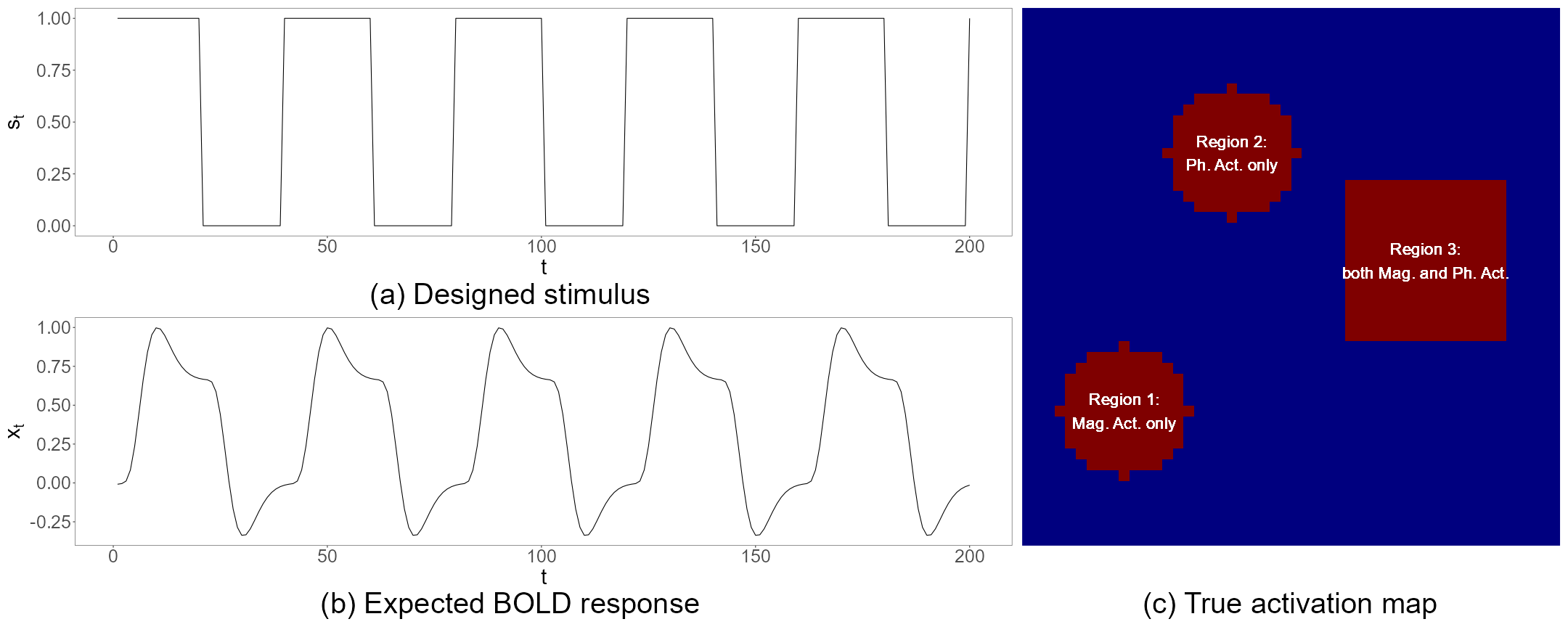
Figure 2: (a) Designed stimulus; (b) Expected BOLD response; (c) True activation map.

3.1.2 True activation map and true strength map

The true activation map contains three active regions on a $50\times 50$ panel, comprising two circles and one square, each with a radius of five. The exact locations of these regions are depicted in Figure 2c. We want to assign distinct types of activation to each region: region 1 exhibits only magnitude activation, region 2 exhibits only phase activation, and region 3 exhibits both magnitude and phase activation, corresponding to the types illustrated in Figures 1a, 1c, and 1b, respectively.

Utilizing the specifyregion function in the neuRosim library (Welvaert et al., 2011) in R (R Core Team, 2023), we initially generate a strength map with decay rates of 0.05, 0.05, and 0.15 for the three regions, respectively. This setup ensures that the central voxel of each active region has a strength of one, diminishing to zero towards the edges at the specified decay rate. For the true magnitude strengths, indicative of voxel response in magnitude to the stimulus, we multiply the strengths in regions 1 and 3 by 0.04909 and nullify the strengths in region 2, as represented in Figure 3c. Similarly, for the true phase strengths, reflective of voxel response in phase, we multiply the strengths in regions 2 and 3 by a factor of $\pi/36$ and reduce the strengths in region 1 to zero, as illustrated in Figure 3g. This methodology ensures that each region’s activation profile is accurately mapped according to its designated stimulus response type.

3.1.3 Simulating fMRI signals

We then simulate data according to Eq. (12):

$$\begin{split}y_{v,Rt}&=(\beta_{0}+x_{t}\beta_{v,1}){\rm cos}(\gamma_{0}+u_{t}\gamma_{v,1})+\varepsilon_{v,Rt},\quad\varepsilon_{v,Rt}\sim\mathcal{N}(0,\sigma^{2}),\\ y_{v,It}&=(\beta_{0}+x_{t}\beta_{v,1}){\rm sin}(\gamma_{0}+u_{t}\gamma_{v,1})+\varepsilon_{v,It},\quad\varepsilon_{v,It}\sim\mathcal{N}(0,\sigma^{2}),\end{split}$$ (12)

where $\beta_{0}=0.4909$, $\gamma_{0}=\pi/4$, and $\sigma=0.04909$ are set constant for all voxels, and $x_{t}$ is the expected BOLD response $\mathbf{x}$ from Figure 2b at time $t$. It should be noted that we also use $\mathbf{u}=\mathbf{x}$ as the regressor for phase here when generating the data, but it could be its own neuronal electromagnetic signal $\mathbf{u}$ for the phase in some cases. The signal-to-noise ratio for the magnitude (SNR${}_{\text{Mag}}$) is thereby fixed at $\beta_{0}/\sigma=10$. The true values of $\beta_{1}$ and $\gamma_{1}$ generated previously in Figures 3c and 3g are used, yielding the contrast-to-noise ratios for magnitude ($\text{CNR}_{\text{Mag}}$) and phase ($\text{CNR}_{\text{Ph}}$) as detailed in Eq. (13):

$$\begin{split}\text{CNR}_{\text{Mag}}&=(\max{\beta_{v,1}})/\sigma=0.04909/0.04909=1,\\ \text{CNR}_{\text{Ph}}&=(\max{\gamma_{v,1}})/{\text{SNR}_{\text{Mag}}}=(\pi/36)/10.\end{split}$$ (13)

3.1.4 Results

Figure 3 presents both the true and estimated activation maps for magnitude and phase as derived from the CV-M&P model, alongside the corresponding true and estimated parameters $\beta_{1}$ and $\gamma_{1}$. Notably, CV-M&P effectively identifies separate regions that are active in magnitude and phase, and provides proper estimates for the parameters $\beta_{1}$ and $\gamma_{1}$. In the estimated activation maps (Figures 3b and 3f), the overlap in the predicted active regions corresponds to the square-shaped region 3 in the true map (Figure 2c), which is characterized by both magnitude and phase activation. When the predicted region 3 is excluded from these estimated maps, the remaining areas align well with the circular regions 1 and 2 in Figure 2c, representing solely magnitude-active and solely phase-active voxels, respectively.

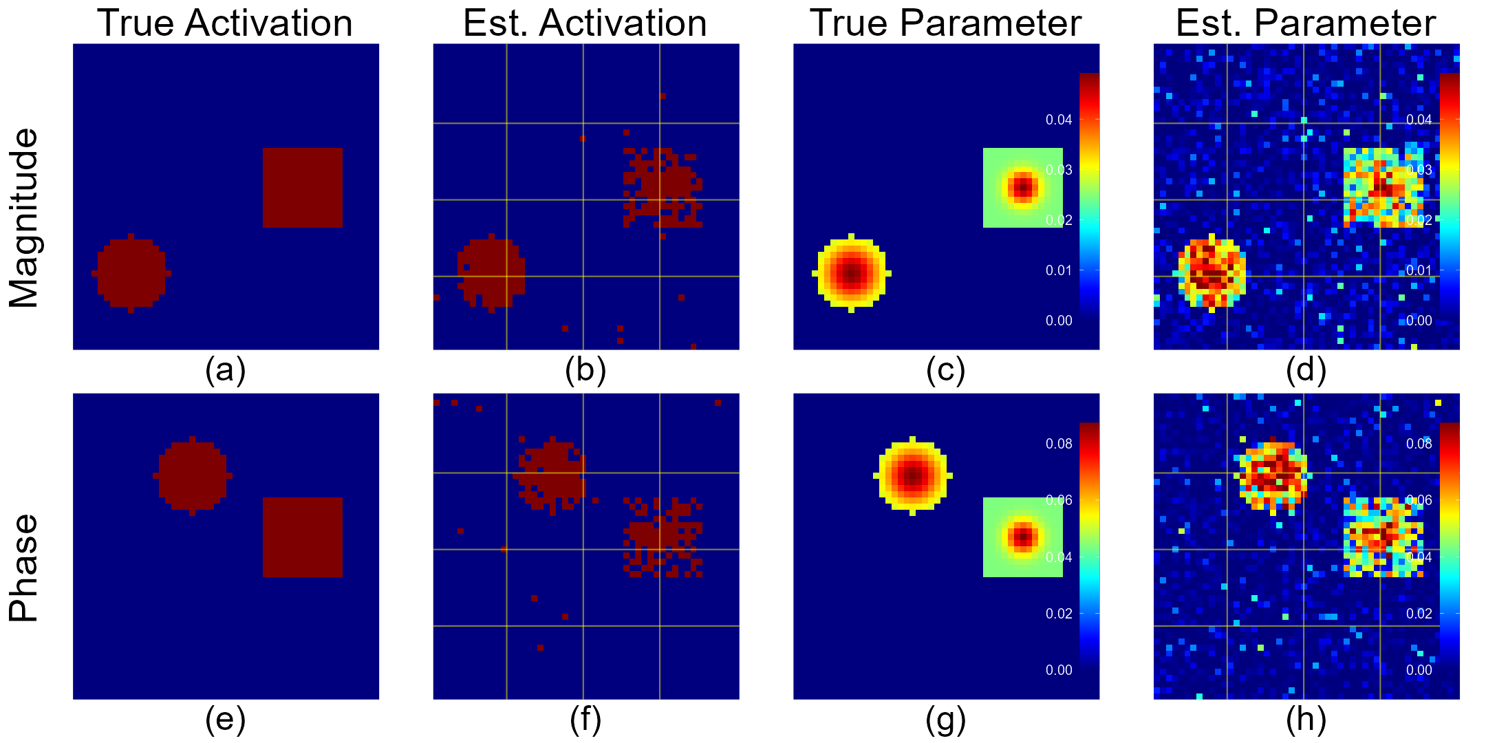
Figure 3: (a) and (e) are true magnitude and phase activation maps; (b) and (f) are estimated activation maps as derived from CV-M&P; (c) and (g) are true $\beta_{1}$ and $\gamma_{1}$; (d) and (h) are estimated $\beta_{1}$ and $\gamma_{1}$ as derived from CV-M&P.

By synthesizing the estimated activation maps for both magnitude and phase (Figures 3b and 3f), we construct a composite activation map and compare it against results from MO and CV-R&I. Figure 4 presents these comparative maps. Performance evaluation reveals that MO fails the competition, primarily due to its inability to detect the phase-only active region 2. Conversely, both CV-R&I and CV-M&P deliver competitive results.

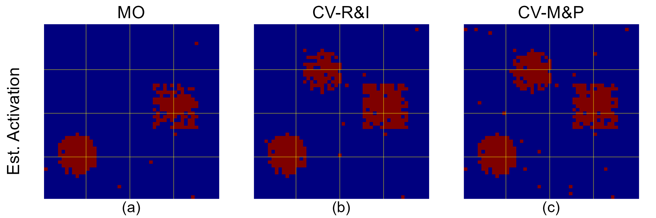
Figure 4: (a)-(c) are estimated activation maps as derived from MO, CV-R&I, and CV-M&P, respectively.

The analysis also extends to comparing the parameter estimations across the three models. As MO and CV-R&I do not explicitly characterize parameters $\beta_{1}$ and $\gamma_{1}$ in their models, we resort to indirect methods for their estimation. For MO model, we use the estimated slope of the BOLD signal, $\widehat{\beta}_{v,M_{1}}$, as an estimate for $\beta_{v,1}$, while for CV-R&I, the square root of the sum of squares of the estimated slopes, $\sqrt{\left(\widehat{\beta}_{v,R_{1}}\right)^{2}+\left(\widehat{\beta}_{v,I_{1}}\right)^{2}}$, serves as an estimate for $\beta_{v,1}$. As for $\gamma_{1}$, MO cannot estimate this parameter due to its limitation to magnitude-only data. In contrast, CV-R&I employs $\text{arctan}_{4}\left(\widehat{\beta}_{v,I_{1}}/\widehat{\beta}_{v,R_{1}}\right)$ as an estimate for $\gamma_{1}$. These results are illustrated in Figure 5. Upon examination of Figure 5a, we observe that while MO’s estimated $\beta_{1}$ map appears to closely align with the true $\beta_{1}$ map (Figure 3c), it still slightly underestimates values in region 3. Similarly, as seen in Figure 5b, CV-R&I not only falsely estimates the non-existent $\beta_{1}$ in the phase-only active region 2, but also tends to overestimate $\beta_{1}$ in region 3. This overestimation of $\beta_{1}$ in region 3 where voxels exhibit both magnitude- and phase-active, is consistent with the findings in Wang et al. (2023). Lastly, Figure 5c reveals the CV-R&I’s estimated $\gamma_{1}$ map significantly deviates from the true $\gamma_{1}$ map, as showcased in Figure 3g.

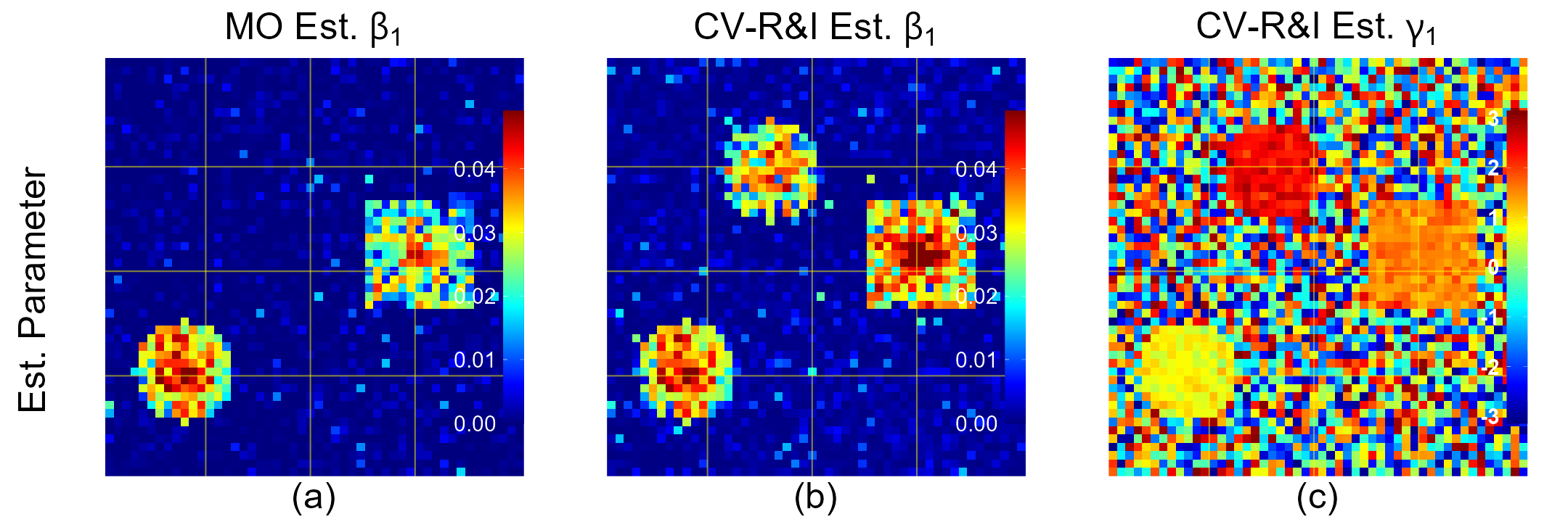
Figure 5: (a)-(c) are improperly estimated parameters as derived from MO and CV-R&I.

The numerical evaluation metrics are summarized in Table 1, where we employ accuracy, precision, recall, F1-score, and the area under the receiver operating characteristic curve (ROC-AUC) to gauge classification performance. We also employ the regression slope between true and estimated parameters to quantify the estimation performance, to expect it be close to one. In terms of classification, CV-M&P outperforms its counterparts in various key metrics, including recall, F1-score, and AUC. While the margin of superiority may not be pronounced, CV-M&P offers two distinct advantages over its counterparts: it allows for the independent prediction of magnitude and phase activation maps, as shown in Figure 3b and 3f, while the other two approaches cannot, and provides accurate estimation for both $\beta_{1}$ and $\gamma_{1}$, as the slopes (0.9731 and 0.9462) are close to one. Further evidence from multiple simulation studies, to be discussed in the subsequent section, will reinforce these findings.

Table 1: Metrics of a single simulated dataset produced by the MO, CV-R&I, and CV-M&P models.

Model	Accuracy	Precision	Recall	F1 Score	AUC	$\beta_{1}$ slope	$\gamma_{1}$ slope	Time (s)
MO	0.9248	0.9726	0.5392	0.6938	0.8910	0.8630	NA	1.54
CV-R&I	0.9688	0.9731	0.8253	0.8931	0.9868	1.0301	33.427	3.93
CV-M&P	0.9680	0.9436	0.8481	0.8933	0.9896	0.9731	0.9462	17.87

3.2 Multiple Simulations

3.2.1 Generating random maps and simulating fMRI signals

We generate 100 random true strength maps using the parameters outlined in Table 2 and the specifyregion function. The true strength maps are then scaled by factors of 0.04909 and $\pi/36$ to obtain 100 true $\beta_{1}$ maps and 100 true $\gamma_{1}$ maps, respectively. Using Eq. (12) and the expected BOLD response $\mathbf{x}$ in Figure 2b, we generate three datasets from each pair of true $\beta_{1}$ and $\gamma_{1}$ maps with the following assignments:

• $\beta_{1}$ present, $\gamma_{1}$ absent (all active voxels are solely magnitude-active)

• $\beta_{1}$ absent, $\gamma_{1}$ present (all active voxels are solely phase-active)

• $\beta_{1}$ present, $\gamma_{1}$ present (all active voxels are both magnitude- and phase-active)

The values for $\beta_{0}$, $\gamma_{0}$, and $\sigma$ are held constant as specified in Section 3.1, with values 0.4909, $\pi/4$, and 0.04909, respectively, resulting $\text{CNR}_{\text{Mag}}=1$ and $\text{CNR}_{\text{Ph}}=(\pi/36)/10$. In total, we have 300 datasets for analysis.

Table 2: Characteristics of true maps.

Map size	Number of active regions	Radius	Shape	Decay rate $(\varrho)$
50$\times$50	3	2 to 6	sphere or cube	0 to 0.3

3.2.2 Results

Table 3 presents the performance metrics for each method across these diverse datasets. In terms of classification, MO delivers superior performance in almost all evaluated metrics for datasets featuring exclusively magnitude-active voxels, which is expected given its design specificity for magnitude-based activity. However, such an assumption of magnitude-only activity is often unrealistic in real-world applications. When considering datasets comprising solely phase-active voxels, CV-M&P excels in all metrics except precision, thereby establishing its superiority in detecting phase-based activity. For mixed activity involving both magnitude and phase, CV-R&I takes the lead in accuracy, precision, and F1-score metrics, whereas CV-M&P dominates in recall and AUC.

Table 3: Summary of average metrics across 100 simulated datasets produced by the MO, CV-R&I, and CV-M&P models. The values in parentheses are min, max, and standard deviation.

Data Type	Measure	MO	CV-R&I	CV-M&P
Mag. -only	Accuracy	0.9645(0.9208, 0.9940, 0.0153)	0.9555(0.9032, 0.9916, 0.0188)	0.9598(0.9132, 0.9900, 0.0160)
	Precision	0.9647(0.9157, 0.9917, 0.0164)	0.9601(0.9078, 0.9964, 0.0166)	0.9317(0.8515, 0.9805, 0.0224)
	Recall	0.7629(0.6052, 0.9680, 0.0707)	0.6966(0.5263, 0.9406, 0.0840)	0.7534(0.6111, 0.9634, 0.0721)
	F1 Score	0.8502(0.7366, 0.9716, 0.0437)	0.8046(0.6741, 0.9515, 0.0557)	0.8311(0.7294, 0.9444, 0.0435)
	AUC	0.9760(0.9485, 0.9991, 0.0107)	0.9605(0.9227, 0.9963, 0.0154)	0.9793(0.9605, 0.9983, 0.0081)
	$\beta_{1}$ slope	0.8696(0.7927, 0.9466, 0.0327)	0.8337(0.7451, 0.9356, 0.0406)	0.9771(0.9337, 1.0170, 0.0190)
	$\gamma_{1}$ slope	NA	NA	NA
Ph. -only	Accuracy	0.8638(0.7576, 0.9428, 0.0418)	0.9390(0.8696, 0.9848, 0.0234)	0.9459(0.8868, 0.9832, 0.0201)
	Precision	0.2102(0.0714, 0.6000, 0.1097)	0.9481(0.8829, 0.9862, 0.0207)	0.9192(0.8324, 0.9735, 0.0303)
	Recall	0.0059(0.0017, 0.0201, 0.0034)	0.5718(0.4207, 0.9026, 0.0970)	0.6481(0.5146, 0.9090, 0.0881)
	F1 Score	0.0114(0.0034, 0.0373, 0.0065)	0.7088(0.5831, 0.9269, 0.0725)	0.7569(0.6456, 0.9225, 0.0604)
	AUC	0.5277(0.4898, 0.6001, 0.0214)	0.9326(0.8844, 0.9930, 0.0237)	0.9544(0.9216, 0.9952, 0.0150)
	$\beta_{1}$ slope	NA	NA	NA
	$\gamma_{1}$ slope	NA	39.813(30.031, 45.799, 3.3285)	0.9439(0.8744, 1.0271, 0.0289)
Both	Accuracy	0.9644(0.9192, 0.9912, 0.0144)	0.9835(0.9616, 0.9984, 0.0071)	0.9769(0.9544, 0.9896, 0.0069)
	Precision	0.9643(0.9017, 0.9892, 0.0146)	0.9798(0.9354, 0.9967, 0.0106)	0.9134(0.7870, 0.9617, 0.0294)
	Recall	0.7606(0.6358, 0.9662, 0.0651)	0.8949(0.8216, 0.9925, 0.0362)	0.9073(0.8457, 0.9927, 0.0329)
	F1 Score	0.8489(0.7703, 0.9592, 0.0398)	0.9350(0.8926, 0.9908, 0.0202)	0.9097(0.8299, 0.9539, 0.0208)
	AUC	0.9763(0.9537, 0.9992, 0.0103)	0.9939(0.9846, 0.9999, 0.0035)	0.9940(0.9873, 0.9997, 0.0026)
	$\beta_{1}$ slope	0.8710(0.7879, 0.9789, 0.0321)	1.2346(1.1693, 1.3360, 0.0305)	0.9843(0.9365, 1.0316, 0.0183)
	$\gamma_{1}$ slope	NA	26.643(19.307, 30.993, 2.4747)	0.9534(0.8958, 1.0146, 0.0253)

CV-M&P once again stands out with respect to parameter estimation. Specifically, its true vs estimated parameter slopes are close to one when the parameters are present in the simulation, indicating accurate estimations. In contrast, this metric from both MO and CV-R&I deviates from the ideal value of one. As explained by Wang et al. (2023), under conditions where all active voxels are solely magnitude-active, the Cartesian model of Lee et al. (2007) and the polar model of Rowe (2005b) (CV-R&I and CV-M&P, respectively) are approximately equivalent. Hence, in such scenario, CV-R&I can properly estimate $\beta_{1}$, although not surpassing the performance of CV-M&P. In other scenarios, both MO and CV-R&I fall short, either failing to estimate $\gamma_{1}$ or inaccurately estimating both $\beta_{1}$ and $\gamma_{1}$.

4 Analysis of Human CV-fMRI Data

In this study, we employ the experimental data previously analyzed by Yu et al. (2018, 2023) and Wang et al. (2023). This dataset originates from a unilateral finger-tapping experiment conducted using a 3.0-Tesla General Electric Signa LX MRI scanner. The experimental design comprises 16.33 epochs, each consisting of alternating periods of 15s on and 15s off. Consequently, the total number of time points is $T=490$, excluding the warm-up phase. The acquired dataset has seven slices, each with dimensions $96\times 96$, and our analysis focuses on the initial six slices. For all examined models, we set the number of parcels $G=25$. Specific tuning parameters are fixed based on the experience: for the MO model, $\psi=\Phi^{-1}(0.02)$; for CV-R&I, $\psi=\Phi^{-1}(0.1)$; and for CV-M&P, $\psi=\omega=\Phi^{-1}(0.20)$. The thresholds for identifying active voxels are set to values as follows: 0.8722 for both MO and CV-R&I, and 0.925 for CV-M&P, in alignment with Section 2.3 and the simulation studies.

In Figure 6, we present the results derived from the CV-M&P model. Distinct patterns are observed: the estimated $\beta_{0}$ maps mirror the patterns of magnitude in the background, the estimated $\gamma_{0}$ maps highlight the phase’s transition lines across different color zones, and both the estimated $\beta_{1}$ and $\gamma_{1}$ maps reflect patterns consistent with the estimated magnitude and phase activation maps. Such patterns are indicative of the accuracy of our approach in both classification and estimation.

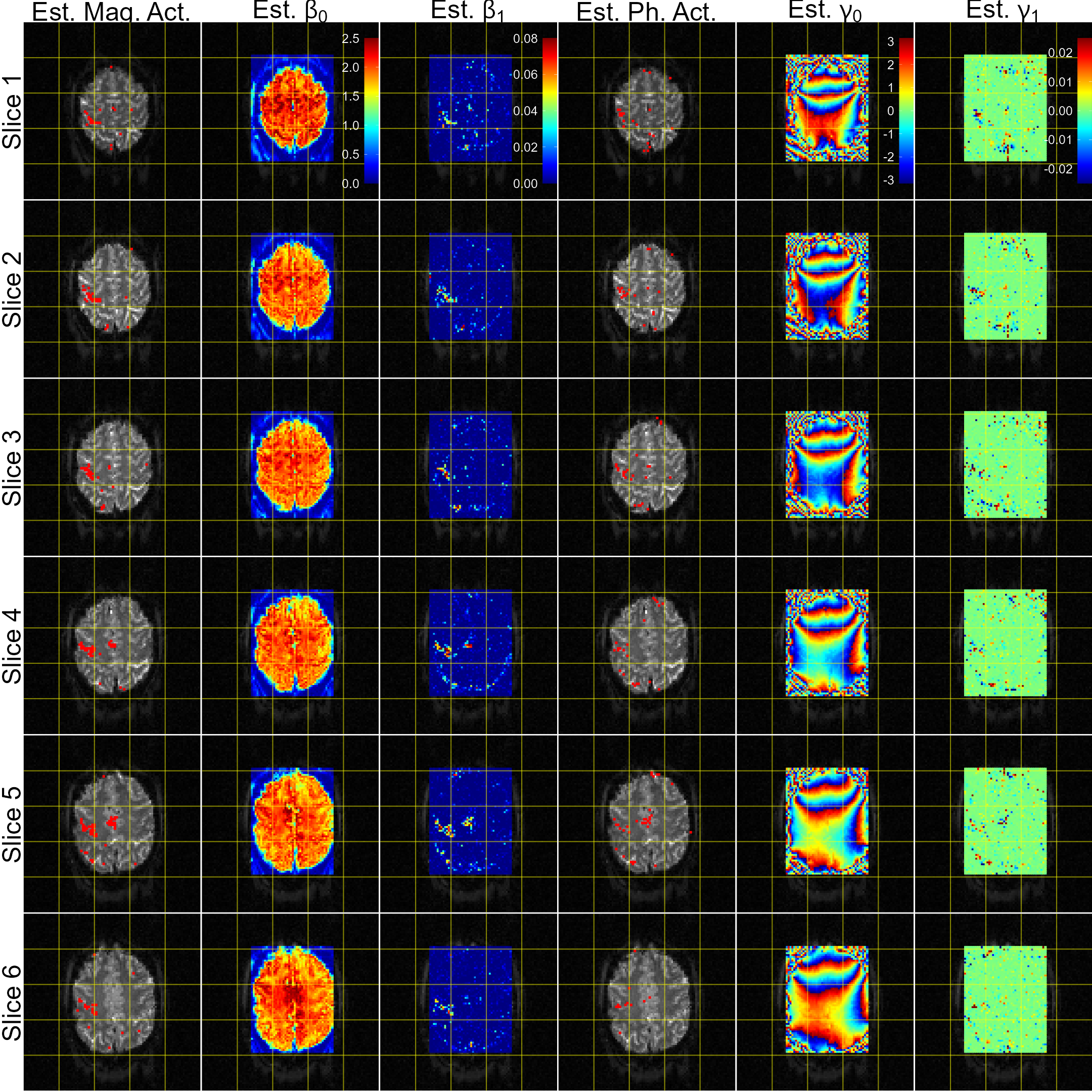
Figure 6: Estimated magnitude activation, $\beta_{0}$, $\beta_{1}$, phase activation, $\gamma_{1}$, $\gamma_{0}$ maps for a real human brain dataset as derived by the CV-M&P model.

By integrating the magnitude- and phase-activation maps derived by CV-M&P model, we form comprehensive estimated activation maps. They are subsequently compared with activation maps estimated by MO and CV-R&I models, as shown in Figure 7, revealing significant alignment. Specifically, the two central and central-left active regions detected by CV-M&P are consistent with the findings reported in Yu et al. (2018, 2023) and Wang et al. (2023). Furthermore, these regions align with known anatomical areas typically activated during finger-tapping tasks. The central region may correspond to the Primary Motor Cortex (M1) or Supplementary Motor Area (SMA), both of which play pivotal roles in voluntary movement and motor planning (Wilder Penfield, 1937; Geyer et al., 1996). Adjacently, the central-left region might represent the Primary Somatosensory Cortex (S1) or the Posterior Parietal Cortex, responsible for tactile sensory information processing and sensory-motor integration, respectively (Culham and Valyear, 2006). Notably, beyond these well-established regions, CV-M&P uncovers additional active regions at the posterior of the brain image. These could be caused by the motion of brain during the data collection.

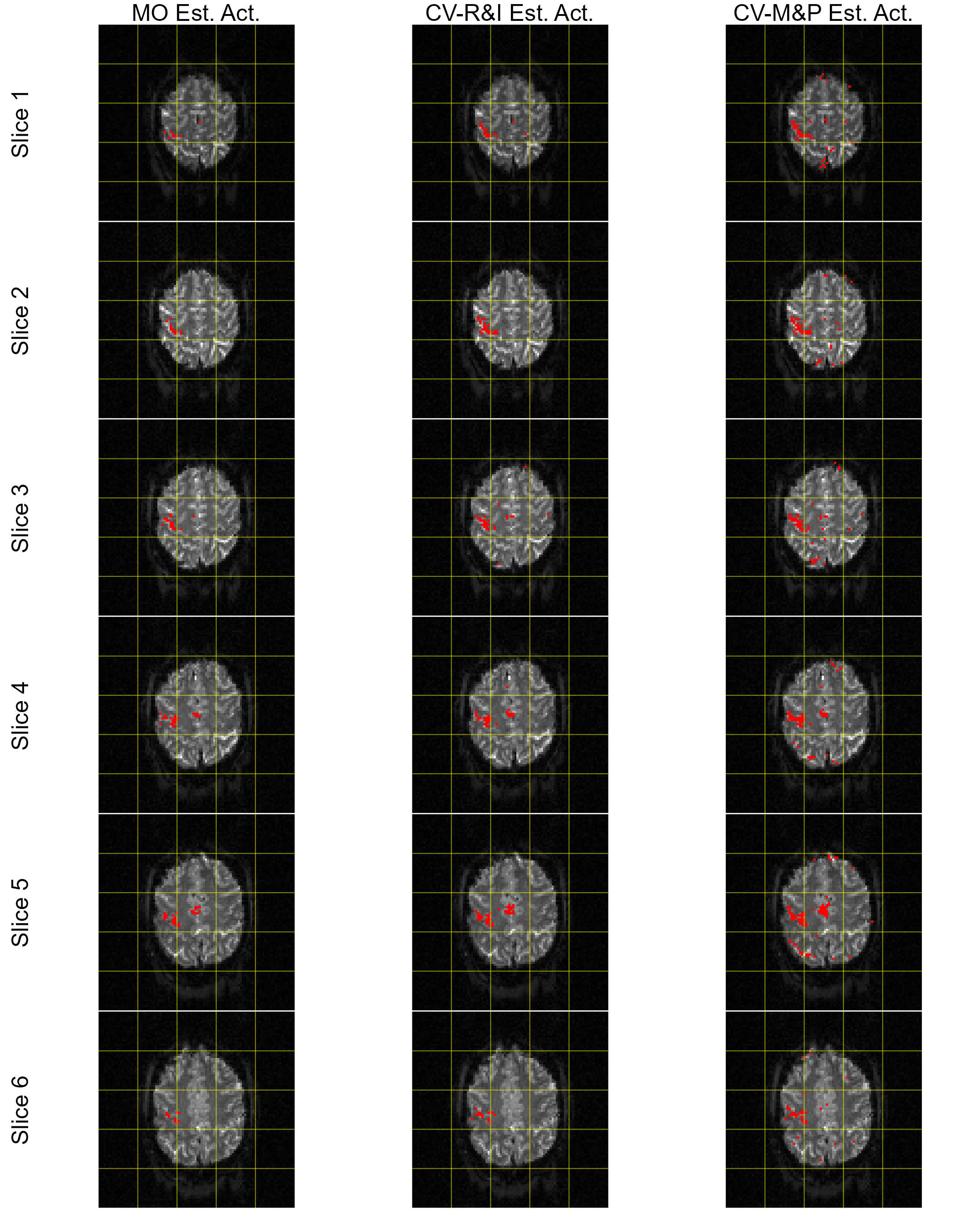
Figure 7: Estimated activation maps for a real human brain dataset as derived by the MO, CV-R&I, and CV-M&P models.

In terms of computational efficiency, MO, CV-R&I, and CV-M&P required 12.32 seconds, 32.59 seconds, and 910.2 seconds, respectively, to complete $10^{3}$ iterations. Despite CV-M&P’s computational demand and increased execution time, its drawbacks are mitigated by its potential for scalability. As highlighted in the works of Musgrove et al. (2016) and Wang et al. (2023), the employment of a brain parcellation strategy along with the sSGLMM spatial prior has minimal effects on the prediction results, as long as the total parcel number $G$ is in a reasonable range. Given that this dataset can be further divided into more parcels for parallel processing, and considering our computational resources are currently limited to 16 CPU cores, the computational efficiency of the CV-M&P model can be substantially improved.

5 Conclusion

Throughout our investigations on both simulated and real human datasets, the CV-M&P model consistently demonstrates its capability to precisely identify voxels that exhibit significant reactions to stimuli, whether in magnitude, in phase, or in a combination of both. Comparing with the polar model of Rowe (2005b), but using hypothesis testing approaches (Rowe and Logan, 2004, 2005; Rowe, 2005b, a; Rowe et al., 2007; Rowe, 2009; Adrian et al., 2018), our fully Bayesian framework can capture the spatial correlations of fMRI data, and therefore improve the model flexibility. On the other hand, comparing with other fully Bayesian approaches, but based on the Cartesian model of Lee et al. (2007) (Yu et al., 2023; Wang et al., 2023), our CV-M&P model rectifies the constraints inherent in the Cartesian models, which can detect active voxels but remains ambiguous about the exact type of the activation (Rowe, 2009). Moreover, the CV-M&P model excels in providing precise parameter estimates, offering a more nuanced framework for delineating brain activation patterns in task-based fMRI analyses.

There are multiple avenues for advancing this research. These include the exploration of more complex models that account for temporal correlations, models that fit the non-circular data wherein the real and imaginary components of the signal are correlated, and efforts aimed at optimizing computational efficiency.

Appendix

Appendix A Conditional Posterior Distributions for Gibbs Sampling

We need the full conditional posterior distributions of

$$\boldsymbol{\beta}_{v},\lambda_{v},\boldsymbol{\gamma}_{v},\omega_{v},\sigma_{v}^{2},\tau_{g}^{2},\xi_{g}^{2},\eta_{\lambda,v},\boldsymbol{\delta}_{\lambda,g},\kappa_{\lambda,g},\eta_{\omega,v},\boldsymbol{\delta}_{\omega,g},\kappa_{\omega,g}$$ (14)

for the Gibbs sampling. All derivations will omit the subscript of $g$ (parcel index) from the parcel-level parameters $\tau_{g}^{2},\xi_{g}^{2},\boldsymbol{\delta}_{\lambda,g},\kappa_{\lambda,g},\boldsymbol{\delta}_{\omega,g},\kappa_{\omega,g}$, since all parcels run the algorithm identically.

A.1 Full conditional distributions of $\lambda_{v}$ and $\omega_{v}$

The full conditional distribution of $\lambda_{v}$ is

$$\pi(\lambda_{v}\mid\mathbf{y}_{r}^{v},\boldsymbol{\beta}_{v},\boldsymbol{\gamma}_{v},\omega_{v},\sigma_{v}^{2},\tau^{2},\xi^{2},\eta_{\lambda,v})={\mathcal{B}}ern\left(P_{\lambda_{v}}\right),$$ (15)

where

$$\begin{split}P_{\lambda_{v}}&=p(\lambda_{v}=1\mid\mathbf{y}_{r}^{v},\boldsymbol{\beta}_{v},\boldsymbol{\gamma}_{v},\omega_{v},\sigma_{v}^{2},\tau^{2},\xi^{2},\eta_{\lambda,v})\\ &=\frac{p(\lambda_{v}=1\mid\eta_{\lambda,v})}{p(\lambda_{v}=1\mid\eta_{\lambda,v})+\frac{L_{0}}{L_{1}}{\cdot}p(\lambda_{v}=0\mid\eta_{\lambda,v})}\\ &=\frac{\mathbf{\Phi}(\psi_{\lambda}+\eta_{\lambda,v})}{\mathbf{\Phi}(\psi_{\lambda}+\eta_{\lambda,v})+\frac{L_{0}}{L_{1}}{\cdot}\left[1-\mathbf{\Phi}(\psi_{\lambda}+\eta_{\lambda,v})\right]},\end{split}$$ (16)

and $L_{0}$ and $L_{1}$ are the joint densities of $\mathbf{y}_{v},\boldsymbol{\beta}_{v},\lambda_{v},\boldsymbol{\gamma}_{v},\omega_{v},\sigma_{v}^{2},\tau^{2},\xi^{2}$ given $\lambda_{v}=0$ and $\lambda_{v}=1$. Let $L$ be such joint density, that is,

$$L=p(\mathbf{y}_{v},\boldsymbol{\beta}_{v},\lambda_{v},\boldsymbol{\gamma}_{v},\omega_{v},\sigma_{v}^{2},\tau^{2},\xi^{2})\propto p(\mathbf{y}_{v}\mid\boldsymbol{\beta}_{v},\lambda_{v},\boldsymbol{\gamma}_{v},\omega_{v},\sigma_{v}^{2})p(\boldsymbol{\beta}_{v}\mid\lambda_{v},\tau^{2}).$$ (17)

Define:

$$\mathbf{A}_{v}=\begin{pmatrix}\mathbf{C}_{v}\\ \mathbf{S}_{v}\\ \end{pmatrix},\quad\text{where }\mathbf{C}_{v}=\text{diag}\left[\cos{\left(\mathbf{U}\mathbf{\Omega}_{v}\boldsymbol{\gamma}_{v}\right)}\right],\quad\mathbf{S}_{v}=\text{diag}\left[\sin{\left(\mathbf{U}\mathbf{\Omega}_{v}\boldsymbol{\gamma}_{v}\right)}\right],\\$$ (18)

(Note, $\mathbf{A}_{v}$ is orthogonal, i.e., $\mathbf{A}_{v}^{\prime}\mathbf{A}_{v}=\mathbf{I}_{2T}$.), then,

$$\begin{split}&\quad p(\mathbf{y}_{v}\mid\boldsymbol{\beta}_{v},\lambda_{v},\boldsymbol{\gamma}_{v},\omega_{v},\sigma_{v}^{2})\\ &=(2\pi\sigma_{v}^{2})^{-\frac{2T}{2}}\exp{\left\{-\frac{1}{2\sigma_{v}^{2}}\left(\mathbf{y}_{v}-\mathbf{A}_{v}\mathbf{X}\mathbf{\Lambda}_{v}\boldsymbol{\beta}_{v}\right)^{\prime}\left(\mathbf{y}_{v}-\mathbf{A}_{v}\mathbf{X}\mathbf{\Lambda}_{v}\boldsymbol{\beta}_{v}\right)\right\}}\\ &=(2\pi\sigma_{v}^{2})^{-\frac{2T}{2}}\exp{\left\{-\frac{1}{2\sigma_{v}^{2}}\left[\mathbf{y}_{v}^{\prime}\mathbf{y}_{v}-2\left(\mathbf{A}_{v}\mathbf{X}\mathbf{\Lambda}_{v}\boldsymbol{\beta}_{v}\right)^{\prime}\mathbf{y}_{v}+\left(\mathbf{\Lambda}_{v}\boldsymbol{\beta}_{v}\right)^{\prime}\mathbf{X}^{\prime}\mathbf{X}\mathbf{\Lambda}_{v}\boldsymbol{\beta}_{v}\right]\right\}},\end{split}$$ (19)

and

$$p(\boldsymbol{\beta}_{v}\mid\lambda_{v},\tau^{2})=(2\pi\tau^{2})^{-\frac{1+\lambda_{v}}{2}}\exp{\left\{-\frac{1}{2\tau^{2}}\boldsymbol{\beta}_{v}^{\prime}\mathbf{\Lambda}_{v}\boldsymbol{\beta}_{v}\right\}}.$$ (20)

Thus,

$$L\propto(2\pi\tau^{2})^{-\frac{1+\lambda_{v}}{2}}\exp{\left\{-\frac{1}{2\sigma_{v}^{2}}\left[-2\left(\mathbf{A}_{v}\mathbf{X}\mathbf{\Lambda}_{v}\boldsymbol{\beta}_{v}\right)^{\prime}\mathbf{y}_{v}+\left(\mathbf{\Lambda}_{v}\boldsymbol{\beta}_{v}\right)^{\prime}\mathbf{X}^{\prime}\mathbf{X}\mathbf{\Lambda}_{v}\boldsymbol{\beta}_{v}\right]-\frac{1}{2\tau^{2}}\boldsymbol{\beta}_{v}^{\prime}\mathbf{\Lambda}_{v}\boldsymbol{\beta}_{v}\right\}}.$$ (21)

Let $\mathbf{a}_{v}$ be the flattened version of $\mathbf{A}_{v}$, that is, $\mathbf{a}_{v}$ is a $2T\times 1$ vector as

$$\mathbf{a}_{v}=\mathbf{A}_{v}\mathbf{1}_{T}=\begin{pmatrix}\cos{\left(\mathbf{U}\mathbf{\Omega}_{v}\boldsymbol{\gamma}_{v}\right)}\\ \sin{\left(\mathbf{U}\mathbf{\Omega}_{v}\boldsymbol{\gamma}_{v}\right)}\end{pmatrix}$$ (22)

Also, define $\mathbf{x}_{(2)}$ as the second column of $\mathbf{X}$, thus, $\mathbf{x}_{(2)}$ is a $T\times 1$ vector of expected BOLD response; define $\mathbf{x}_{(2)}^{*}=\begin{pmatrix}\mathbf{x}_{(2)}\\ \mathbf{x}_{(2)}\end{pmatrix}$ as a $2T\times 1$ vector to match the dimension, then,

$$\begin{split}\frac{L_{0}}{L_{1}}&=\frac{L\mid_{\lambda_{v}=0}}{L\mid_{\lambda_{v}=1}}\\ &=(2\pi\tau^{2})^{\frac{1}{2}}\exp{\left\{-\frac{1}{2\sigma_{v}^{2}}\left[2\beta_{v,1}\left(\mathbf{x}_{(2)}^{*}\odot\mathbf{a}_{v}\right)^{\prime}\mathbf{y}_{v}-2\beta_{v,0}\beta_{v,1}\mathbf{x}_{(2)}^{\prime}\mathbf{1}_{T}-\beta_{v,1}^{2}\mathbf{x}_{(2)}^{\prime}\mathbf{x}_{(2)}\right]+\frac{1}{2\tau^{2}}\beta_{v,1}^{2}\right\}}.\end{split}$$ (23)

We flatten $\mathbf{A}_{v}$ and use Hadamard product $\odot$ here to lessen the computational burden. Similarly, the full conditional distribution of $\omega_{v}$ is

$$\pi(\omega_{v}\mid\mathbf{y}_{r}^{v},\boldsymbol{\beta}_{v},\lambda_{v},\boldsymbol{\gamma}_{v},\sigma_{v}^{2},\tau^{2},\xi^{2},\eta_{v})={\mathcal{B}}ern\left(P_{\omega_{v}}\right),$$ (24)

where

$$P_{\omega_{v}}=\frac{\mathbf{\Phi}(\psi_{\omega}+\eta_{\omega,v})}{\mathbf{\Phi}(\psi_{\omega}+\eta_{\omega,v})+\frac{L_{0}}{L_{1}}{\cdot}\left[1-\mathbf{\Phi}(\psi_{\omega}+\eta_{\omega,v})\right]},$$ (25)

where

$$L\propto(2\pi\xi^{2})^{-\frac{1+\omega_{v}}{2}}\exp{\left\{\frac{1}{\sigma_{v}^{2}}\left(\mathbf{A}_{v}\mathbf{X}\mathbf{\Lambda}_{v}\boldsymbol{\beta}_{v}\right)^{\prime}\mathbf{y}_{v}-\frac{1}{2\xi^{2}}\boldsymbol{\gamma}_{v}^{\prime}\mathbf{\Omega}_{v}\boldsymbol{\gamma}_{v}\right\}},$$ (26)

and

$$\begin{split}\frac{L_{0}}{L_{1}}&=\frac{L\mid_{\omega_{v}=0}}{L\mid_{\omega_{v}=1}}\\ &=(2\pi\xi^{2})^{\frac{1}{2}}\exp{\left\{\frac{1}{\sigma_{v}^{2}}\left[\left(\mathbf{A}_{v}\mid_{\omega_{v}=0}-\mathbf{A}_{v}\mid_{\omega_{v}=1}\right)\mathbf{X}\mathbf{\Lambda}_{v}\boldsymbol{\beta}_{v}\right]^{\prime}\mathbf{y}_{v}+\frac{1}{2\xi^{2}}\gamma_{v,1}^{2}\right\}}.\end{split}$$ (27)

Keep simplifying it, when $\lambda_{v}=0$,

$$\frac{L_{0}}{L_{1}}=(2\pi\xi^{2})^{\frac{1}{2}}\exp{\left\{\frac{1}{\sigma_{v}^{2}}\beta_{v,0}\left(\mathbf{a}_{v}\mid_{\omega_{v}=0}-\mathbf{a}_{v}\mid_{\omega_{v}=1}\right)^{\prime}\mathbf{y}_{v}+\frac{1}{2\xi^{2}}\gamma_{v,1}^{2}\right\}}.$$ (28)

When $\lambda_{v}=1$,

$$\frac{L_{0}}{L_{1}}=(2\pi\xi^{2})^{\frac{1}{2}}\exp{\left\{\frac{1}{\sigma_{v}^{2}}\left[\left(\beta_{v,0}\mathbf{1}_{2T}+\beta_{v,1}\mathbf{x}_{(2)}^{*}\right)\odot\left(\mathbf{a}_{v}\mid_{\omega_{v}=0}-\mathbf{a}_{v}\mid_{\omega_{v}=1}\right)\right]^{\prime}\mathbf{y}_{v}+\frac{1}{2\xi^{2}}\gamma_{v,1}^{2}\right\}}.$$ (29)

A.2 Full conditional distribution of $\boldsymbol{\beta}_{v}$

When $\lambda_{v}=1$, the full conditional distribution of $\boldsymbol{\beta}_{v}$ is

$$\begin{split}&\quad\pi(\boldsymbol{\beta}_{v}\mid\mathbf{y}_{v},\lambda_{v}=1,\boldsymbol{\gamma}_{v},\omega_{v},\sigma_{v}^{2},\tau^{2},\xi^{2})\\ &\propto p(\mathbf{y}_{v},\boldsymbol{\beta}_{v},\lambda_{v}=1,\boldsymbol{\gamma}_{v},\omega_{v},\sigma_{v}^{2},\tau^{2},\xi^{2})\\ &\propto p(\mathbf{y}_{v}\mid\boldsymbol{\beta}_{v},\lambda_{v}=1,\boldsymbol{\gamma}_{v},\omega_{v},\sigma_{v}^{2})p(\boldsymbol{\beta}_{v}\mid\lambda_{v}=1,\tau^{2})\\ &\propto\exp{\left\{-\frac{1}{2\sigma_{v}^{2}}\left(\mathbf{y}_{v}-\mathbf{A}_{v}\mathbf{X}\boldsymbol{\beta}_{v}\right)^{\prime}\left(\mathbf{y}_{v}-\mathbf{A}_{v}\mathbf{X}\boldsymbol{\beta}_{v}\right)\right\}}\exp{\left\{-\frac{1}{2\tau^{2}}\boldsymbol{\beta}_{v}^{\prime}\boldsymbol{\beta}_{v}\right\}}\\ &\propto\exp{\left\{-\frac{1}{2}\left[\boldsymbol{\beta}_{v}^{\prime}\frac{\left(\mathbf{A}_{v}\mathbf{X}\right)^{\prime}\left(\mathbf{A}_{v}\mathbf{X}\right)}{\sigma_{v}^{2}}\boldsymbol{\beta}_{v}-2\boldsymbol{\beta}_{v}^{\prime}\frac{\left(\mathbf{A}_{v}\mathbf{X}\right)^{\prime}}{\sigma_{v}^{2}}\mathbf{y}_{v}+\boldsymbol{\beta}_{v}^{\prime}\frac{1}{\tau^{2}}\boldsymbol{\beta}_{v}\right]\right\}}\\ &=\exp{\left\{-\frac{1}{2}\left[\boldsymbol{\beta}_{v}^{\prime}\frac{\left(\mathbf{A}_{v}\mathbf{X}\right)^{\prime}\left(\mathbf{A}_{v}\mathbf{X}\right)+\frac{\sigma_{v}^{2}}{\tau^{2}}\mathbf{I}}{\sigma_{v}^{2}}\boldsymbol{\beta}_{v}-2\boldsymbol{\beta}_{v}^{\prime}\frac{\left(\mathbf{A}_{v}\mathbf{X}\right)^{\prime}}{\sigma_{v}^{2}}\mathbf{y}_{v}\right]\right\}}\\ &=\exp{\left\{-\frac{1}{2}\left[\boldsymbol{\beta}_{v}^{\prime}\frac{\mathbf{X}^{\prime}\mathbf{X}+\frac{\sigma_{v}^{2}}{\tau^{2}}\mathbf{I}}{\sigma_{v}^{2}}\boldsymbol{\beta}_{v}-2\boldsymbol{\beta}_{v}^{\prime}\frac{\left(\mathbf{A}_{v}\mathbf{X}\right)^{\prime}}{\sigma_{v}^{2}}\mathbf{y}_{v}\right]\right\}}.\end{split}$$ (30)

Therefore,

$$\pi(\boldsymbol{\beta}_{v}\mid\mathbf{y}_{v},\lambda_{v}=1,\boldsymbol{\gamma}_{v},\omega_{v},\sigma_{v}^{2},\tau^{2},\xi^{2})=\mathcal{N}_{2}(\boldsymbol{\mu}_{\boldsymbol{\beta}_{v}},\boldsymbol{\Sigma}_{\boldsymbol{\beta}_{v}}),$$ (31)

where

$$\begin{split}\boldsymbol{\mu}_{\boldsymbol{\beta}_{v}}&=\left(\mathbf{X}^{\prime}\mathbf{X}+\frac{\sigma_{v}^{2}}{\tau^{2}}\mathbf{I}\right)^{-1}\left(\mathbf{A}_{v}\mathbf{X}\right)^{\prime}\mathbf{y}_{v},\\ \boldsymbol{\Sigma}_{\boldsymbol{\beta}_{v}}&=\sigma_{v}^{2}\left(\mathbf{X}^{\prime}\mathbf{X}+\frac{\sigma_{v}^{2}}{\tau^{2}}\mathbf{I}\right)^{-1},\end{split}$$ (32)

where $\mathbf{A}_{v}\mathbf{X}$ can be calculated as $\left[\mathbf{a}_{v},\mathbf{x}_{(2)}^{*}\odot\mathbf{a}_{v}\right]$ for faster computation. When $\lambda_{v}=0$, it’s easy to show:

$$\pi(\boldsymbol{\beta}_{v,0}\mid\mathbf{y}_{v},\lambda_{v}=0,\boldsymbol{\gamma}_{v},\omega_{v},\sigma_{v}^{2},\tau^{2},\xi^{2})=\mathcal{N}(\frac{\left(\mathbf{A}_{v}\mathbf{1}_{T}\right)^{\prime}\mathbf{y}_{v}}{T+\frac{\sigma_{v}^{2}}{\tau^{2}}},\frac{\sigma_{v}^{2}}{T+\frac{\sigma_{v}^{2}}{\tau^{2}}}),$$ (33)

and $\boldsymbol{\beta}_{v,1}=0$ with probability 1, where $\mathbf{A}_{v}\mathbf{1}_{T}$ is just $\mathbf{a}_{v}$.

A.3 Sampling $\boldsymbol{\gamma}_{v}$

We apply Metropolis-Hastings algorithm to sample $\boldsymbol{\gamma}_{v}$. A random walk proposal,

$$\boldsymbol{\gamma}_{v}^{*}\mid\boldsymbol{\gamma}_{v}\sim\mathcal{N}_{2}\left(\mathbf{\Omega}_{v}\boldsymbol{\gamma}_{v},\quad\mathbf{\Omega}_{v}^{\prime}\boldsymbol{\Sigma}_{\boldsymbol{\gamma}_{v}}\mathbf{\Omega}_{v}\right),$$ (34)

is used, where $\boldsymbol{\gamma}_{v}^{*}$ and $\boldsymbol{\gamma}_{v}$ are proposed parameter and current state, respectively, and $\boldsymbol{\Sigma}_{\boldsymbol{\gamma}_{v}}$ is a tuning parameter. We use the current indicator of phase status, $\mathbf{\Omega}_{v}$, to secure it proposes $\boldsymbol{\gamma}_{v}^{*}=\begin{pmatrix}\gamma_{v,0}^{*}\neq 0\\ \gamma_{v,1}^{*}=0\end{pmatrix}$ when the phase is inactive. Let $p_{\boldsymbol{\gamma}_{v}}(\cdot)$ be the proposal density, then the acceptance ratio is

$$\begin{split}r_{\boldsymbol{\gamma}_{v}}&=\frac{\pi(\boldsymbol{\gamma}_{v}^{*}\mid\mathbf{y}_{v},\boldsymbol{\beta}_{v},\lambda_{v},\omega_{v},\sigma_{v}^{2},\tau^{2},\xi^{2})p_{\boldsymbol{\gamma}_{v}}(\boldsymbol{\gamma}_{v}\mid\boldsymbol{\gamma}_{v}^{*})}{\pi(\boldsymbol{\gamma}_{v}\mid\mathbf{y}_{v},\boldsymbol{\beta}_{v},\lambda_{v},\omega_{v},\sigma_{v}^{2},\tau^{2},\xi^{2})p_{\boldsymbol{\gamma}_{v}}(\boldsymbol{\gamma}_{v}^{*}\mid\boldsymbol{\gamma}_{v})}\\ &=\frac{p(\mathbf{y}_{v}\mid\boldsymbol{\beta}_{v},\lambda_{v},\boldsymbol{\gamma}_{v}^{*},\omega_{v},\sigma_{v}^{2})p(\boldsymbol{\gamma}_{v}^{*}\mid\omega_{v},\xi^{2})}{p(\mathbf{y}_{v}\mid\boldsymbol{\beta}_{v},\lambda_{v},\boldsymbol{\gamma}_{v},\omega_{v},\sigma_{v}^{2})p(\boldsymbol{\gamma}_{v}\mid\omega_{v},\xi^{2})},\end{split}$$ (35)

where

$$\begin{split}p(\mathbf{y}_{v}\mid\boldsymbol{\beta}_{v},\lambda_{v},\boldsymbol{\gamma}_{v},\omega_{v},\sigma_{v}^{2})&\propto\exp{\left\{-\frac{1}{2\sigma_{v}^{2}}\left(\mathbf{y}_{v}-\mathbf{A}_{v}\mathbf{X}\mathbf{\Lambda}_{v}\boldsymbol{\beta}_{v}\right)^{\prime}\left(\mathbf{y}_{v}-\mathbf{A}_{v}\mathbf{X}\mathbf{\Lambda}_{v}\boldsymbol{\beta}_{v}\right)\right\}}\\ &\propto\exp{\left\{\frac{1}{\sigma_{v}^{2}}\left(\mathbf{A}_{v}\mathbf{X}\mathbf{\Lambda}_{v}\boldsymbol{\beta}_{v}\right)^{\prime}\mathbf{y}_{v}\right\}},\\ p(\boldsymbol{\gamma}_{v}\mid\omega_{v},\xi^{2})&\propto\exp{\left\{-\frac{1}{2\xi^{2}}\boldsymbol{\gamma}_{v}^{\prime}\mathbf{\Omega}_{v}\boldsymbol{\gamma}_{v}\right\}}.\end{split}$$ (36)

Simplify the ratio, when $\lambda_{v}=0$,

$$r_{\boldsymbol{\gamma}_{v}}=\exp{\left\{\frac{1}{\sigma_{v}^{2}}\beta_{v,0}\left(\mathbf{a}_{v}\mid_{\boldsymbol{\gamma}_{v}=\boldsymbol{\gamma}_{v}^{*}}-\mathbf{a}_{v}\mid_{\boldsymbol{\gamma}_{v}=\boldsymbol{\gamma}_{v}}\right)^{\prime}\mathbf{y}_{v}-\frac{1}{2\xi^{2}}\left(\gamma_{v,0}^{*,2}-\gamma_{v,0}^{2}\right)\right\}}.$$ (37)

When $\lambda_{v}=1$,

$$r_{\boldsymbol{\gamma}_{v}}=\exp{\left\{\frac{1}{\sigma_{v}^{2}}\left[\left(\beta_{v,0}\mathbf{1}_{2T}+\beta_{v,1}\mathbf{x}_{(2)}^{*}\right)\odot\left(\mathbf{a}_{v}\mid_{\boldsymbol{\gamma}_{v}=\boldsymbol{\gamma}_{v}^{*}}-\mathbf{a}_{v}\mid_{\boldsymbol{\gamma}_{v}=\boldsymbol{\gamma}_{v}}\right)\right]^{\prime}\mathbf{y}_{v}-\frac{1}{2\xi^{2}}\left(\boldsymbol{\gamma}_{v}^{*^{\prime}}\boldsymbol{\gamma}_{v}^{*}-\boldsymbol{\gamma}_{v}^{\prime}\boldsymbol{\gamma}_{v}\right)\right\}}.$$ (38)

We generate a dummy variable $d_{\boldsymbol{\gamma}_{v}}\sim\mathcal{U}(0,1)$, and if $d_{\boldsymbol{\gamma}_{v}}<r_{\boldsymbol{\gamma}_{v}}$, we update $\boldsymbol{\gamma}_{v}$ by $\boldsymbol{\gamma}_{v}^{*}$, otherwise remain $\boldsymbol{\gamma}_{v}$.

A.4 Full conditional distribution of $\sigma_{v}^{2}$

Assigning a Jeffreys prior, $p(\sigma_{v}^{2})\propto 1/\sigma_{v}^{2}$, we have:

$$\pi(\sigma_{v}^{2}\mid\mathbf{y}_{v},\cdot)=\mathcal{I}\mathcal{G}\left(\frac{2T}{2},\quad\frac{1}{2}\left(\mathbf{y}_{v}-\mathbf{A}_{v}\mathbf{X}\mathbf{\Lambda}_{v}\boldsymbol{\beta}_{v}\right)^{\prime}\left(\mathbf{y}_{v}-\mathbf{A}_{v}\mathbf{X}\mathbf{\Lambda}_{v}\boldsymbol{\beta}_{v}\right)\right).$$ (39)

Again, to save computational time, $\mathbf{A}_{v}\mathbf{X}\mathbf{\Lambda}_{v}\boldsymbol{\beta}_{v}$ can be calculated as $\beta_{v,0}\mathbf{a}_{v}$ when $\lambda_{v}=0$, or $\left(\beta_{v,0}\mathbf{1}_{2T}+\beta_{v,1}\mathbf{x}_{(2)}^{*}\right)\odot\mathbf{a}_{v}$ when $\lambda_{v}=1$.

A.5 Full conditional distributions of $\tau^{2}$ and $\xi^{2}$

The full conditional distribution of $\tau^{2}$ should be related to all voxels’ $\beta_{0}$’s and magnitude-active voxels’ $\beta_{1}$’s. Assigning a Jeffreys prior, $p(\tau^{2})\propto 1/\tau^{2}$, we have:

$$\pi(\tau^{2}\mid\mathbf{y}_{v},\cdot)=\mathcal{I}\mathcal{G}\left(\frac{1}{2}\sum_{v=1}^{V}\mathbf{1}_{2}^{\prime}\mathbf{\Lambda}_{v}\mathbf{1}_{2},\quad\frac{1}{2}\sum_{v=1}^{V}\boldsymbol{\beta}_{v}^{\prime}\mathbf{\Lambda}_{v}\boldsymbol{\beta}_{v}\right).$$ (40)

Equivalently,

$$\pi(\tau^{2}\mid\mathbf{y}_{v},\cdot)=\mathcal{I}\mathcal{G}\left(\frac{1}{2}\left(V+\sum_{v=1}^{V}\lambda_{v}\right),\quad\frac{1}{2}\sum_{v=1}^{V}\left[\beta_{v,0}^{2}+\left(\lambda_{v}\beta_{v,1}\right)^{2}\right]\right).$$ (41)

Similarly, the full conditional distribution of $\xi^{2}$ should be related to all voxels’ $\gamma_{0}$’s and phase-active voxels’ $\gamma_{1}$’s, that is,

$$\pi(\xi^{2}\mid\mathbf{y}_{v},\cdot)=\mathcal{I}\mathcal{G}\left(\frac{1}{2}\sum_{v=1}^{V}\mathbf{1}_{2}^{\prime}\mathbf{\Omega}_{v}\mathbf{1}_{2},\quad\frac{1}{2}\sum_{v=1}^{V}\boldsymbol{\gamma}_{v}^{\prime}\mathbf{\Omega}_{v}\boldsymbol{\gamma}_{v}\right).$$ (42)

Equivalently,

$$\pi(\xi^{2}\mid\mathbf{y}_{v},\cdot)=\mathcal{I}\mathcal{G}\left(\frac{1}{2}\left(V+\sum_{v=1}^{V}\omega_{v}\right),\quad\frac{1}{2}\sum_{v=1}^{V}\left[\gamma_{v,0}^{2}+\left(\omega_{v}\gamma_{v,1}\right)^{2}\right]\right).$$ (43)

A.6 Full conditional distributions of $\eta_{v}$, $\boldsymbol{\delta}$, and $\kappa$

Let $\mathbf{Q}_{s}=\mathbf{M}^{\prime}\mathbf{Q}\mathbf{M}$. then we follow the supplementary material in Wang et al. [2023], we have:

$$\pi(\eta_{\lambda,v}\mid\lambda_{v},\kappa_{\lambda})=\begin{cases}\mathcal{T}\mathcal{N}(0,\;\frac{1}{\kappa_{\lambda}}\left(1+\mathbf{m}_{v}{{}^{\prime}}\mathbf{Q}_{s}^{-1}\mathbf{m}_{v}\right),\;0,\;\infty)&{{\rm if}\;\lambda_{v}=1}\\ \mathcal{T}\mathcal{N}(0,\;\frac{1}{\kappa_{\lambda}}\left(1+\mathbf{m}_{v}{{}^{\prime}}\mathbf{Q}_{s}^{-1}\mathbf{m}_{v}\right),\;-\infty,\;0)&{{\rm if}\;\lambda_{v}=0}\end{cases},$$ (44)

$$\pi(\eta_{\omega,v}\mid\omega_{v},\kappa_{\omega})=\begin{cases}\mathcal{T}\mathcal{N}(0,\;\frac{1}{\kappa_{\omega}}\left(1+\mathbf{m}_{v}{{}^{\prime}}\mathbf{Q}_{s}^{-1}\mathbf{m}_{v}\right),\;0,\;\infty)&{{\rm if}\;\omega_{v}=1}\\ \mathcal{T}\mathcal{N}(0,\;\frac{1}{\kappa_{\omega}}\left(1+\mathbf{m}_{v}{{}^{\prime}}\mathbf{Q}_{s}^{-1}\mathbf{m}_{v}\right),\;-\infty,\;0)&{{\rm if}\;\omega_{v}=0}\end{cases},$$ (45)

where $\mathcal{T}\mathcal{N}$ denotes the truncated normal distribution. Let $\boldsymbol{\eta}_{\lambda}=(\eta_{\lambda,1},\ldots,\eta_{{\lambda,V}})^{\prime}$ and $\boldsymbol{\eta}_{\omega}=(\eta_{\omega,1},\ldots,\eta_{{\omega,V}})^{\prime}$, then:

$$\pi(\boldsymbol{\delta}_{\lambda}\mid\boldsymbol{\eta}_{\lambda},\kappa_{\lambda})=\mathcal{N}_{q}\left(\frac{1}{\kappa_{\lambda}}\left(\mathbf{Q}_{s}+\mathbf{M}{{}^{\prime}}\mathbf{M}\right)^{-1}\mathbf{M}{{}^{\prime}}\boldsymbol{\eta}_{\lambda},\quad\frac{1}{\kappa_{\lambda}}\left(\mathbf{Q}_{s}+\mathbf{M}{{}^{\prime}}\mathbf{M}\right)^{-1}\right),$$ (46)

$$\pi(\boldsymbol{\delta}_{\omega}\mid\boldsymbol{\eta}_{\omega},\kappa_{\omega})=\mathcal{N}_{q}\left(\frac{1}{\kappa_{\omega}}\left(\mathbf{Q}_{s}+\mathbf{M}{{}^{\prime}}\mathbf{M}\right)^{-1}\mathbf{M}{{}^{\prime}}\boldsymbol{\eta}_{\omega},\quad\frac{1}{\kappa_{\omega}}\left(\mathbf{Q}_{s}+\mathbf{M}{{}^{\prime}}\mathbf{M}\right)^{-1}\right).$$ (47)

Moreover,

$$\pi(\kappa_{\lambda}\mid\boldsymbol{\eta}_{\lambda})=\mathcal{G}amma\left(a=\frac{V+1}{2},\quad b=\left[\frac{1}{2}\left(\sum_{v=1}^{V}\frac{\eta_{\lambda,v}^{2}}{(1+\mathbf{m}_{v}{{}^{\prime}}\mathbf{Q}_{s}^{-1}\mathbf{m}_{v})}\right)+\frac{1}{2000}\right]^{-1}\right),$$ (48)

$$\pi(\kappa_{\omega}\mid\boldsymbol{\eta}_{\omega})=\mathcal{G}amma\left(a=\frac{V+1}{2},\quad b=\left[\frac{1}{2}\left(\sum_{v=1}^{V}\frac{\eta_{\omega,v}^{2}}{(1+\mathbf{m}_{v}{{}^{\prime}}\mathbf{Q}_{s}^{-1}\mathbf{m}_{v})}\right)+\frac{1}{2000}\right]^{-1}\right),$$ (49)

where $b$ is the scale.

References

- Adrian et al. [2018] Daniel W. Adrian, Ranjan Maitra, and Daniel B. Rowe. Complex-valued time series modeling for improved activation detection in fmri studies. Annals of Applied Statistics, 12(3):1451–1478, 2018.
- Boynton et al. [1996] Geoffrey M. Boynton, Stephen A. Engel, Gary H. Glover, and David J. Heeger. Linear systems analysis of functional magnetic resonance imaging in human v1. Journal of Neuroscience, 16(13):4207–4221, 1996.
- Brown et al. [2014] Robert W. Brown, Yu-Chung N. Cheng, E. Mark Haacke, Michael R. Thompson, and Ramesh Venkatesan. Magnetic Resonance Imaging: Physical Principles and Sequence Design. John Wiley & Sons, Inc., Hoboken, New Jersey, 2nd edition, 2014.
- Culham and Valyear [2006] Jody C. Culham and Kenneth F. Valyear. Human parietal cortex in action. Current Opinion in Neurobiology, 16(2):205–212, 2006.
- Epstein and Kanwisher [1998] Russell Epstein and Nancy Kanwisher. A cortical representation of the local visual environment. Nature, 392(6676):598–601, 1998.
- Feng et al. [2009] Zhaomei Feng, Arvind Caprihan, Krastan B. Blagoev c, and Vince D. Calhoun. Biophysical modeling of phase changes in BOLD fMRI. NeuroImage, 47(2):540–548, 2009.
- Flegal et al. [2008] James M. Flegal, Murali Haran, and Galin L. Jones. Markov chain monte carlo: can we trust the third significant figure? Statistical Science, 23(2):250–260, 2008.
- Friston et al. [1994] K. J. Friston, A. P. Holmes, K. J. Worsley, J.-P. Poline, C. D. Frith, and R. S. J. Frackowiak. Statistical parametric maps in functional imaging: A general linear approach. Human Brain Mapping, 2(4):189–210, 1994.
- Gelfand and Smith [1990] A. E. Gelfand and A. F. M. Smith. Sampling-based approaches to calculating marginal densities. Journal of the American Statistical Association, 85(410):398–409, 1990.
- Geyer et al. [1996] Stefan Geyer, Anders Ledberg, Axel Schleicher, Shigeo Kinomura, Thorsten Schormann, Uli Bürgel, Torkel Klingberg, Jonas Larsson, Karl Zilles, and Per E. Roland. Two different areas within the primary motor cortex of man. Nature, 382(6594):805–807, 1996.
- Gudbjartsson and Patz [1995] Hákon Gudbjartsson and Samuel Patz. The rician distribution of noisy mri data. Magnetic Resonance in Medicine, 34(6):910–914, 1995.
- Hastings [1970] W. K. Hastings. Monte Carlo sampling methods using Markov chains and their applications. Biometrika, 57(1):97–109, 1970.
- Hughes and Haran [2013] John Hughes and Murali Haran. Dimension reduction and alleviation of confounding for spatial generalized linear mixed models. Journal of the Royal Statistical Society. Series B (Statistical Methodology), 75(1):139–159, 2013.
- Karaman et al. [2014] Muge Karaman, Andrew S. Nencka, Iain P. Bruce, and Daniel B. Rowe. Quantification of the statistical effects of spatiotemporal processing of nontask FMRI data. Brain Connectivity, 4(9):649–661, 2014.
- Lee et al. [2007] Jongho Lee, Morteza Shahram, Armin Schwartzman, and John M. Pauly. Complex data analysis in high-resolution ssfp fmri. Magnetic Resonance in Medicine, 57(5):905–917, 2007.
- Lindquist [2008] Martin A. Lindquist. The statistical analysis of fmri data. Statistical Science, 23(4):439–464, 2008.
- Logothetis [2008] Nikos K. Logothetis. What we can do and what we cannot do with fMRI. Nature, 453(7197):869–878, 2008.
- Metropolis et al. [1953] Nicholas Metropolis, Arianna W. Rosenbluth, Marshall N. Rosenbluth, Augusta H. Teller, and Edward Teller. Equation of state calculations by fast computing machines. Journal of Chemical Physics, 21(6):1087–1092, 1953.
- Mitchell and Beauchamp [1988] T. J. Mitchell and J. J. Beauchamp. Bayesian variable selection in linear regression. Journal of the American Statistical Association, 83(404):1023–1032, 1988.
- Musgrove et al. [2016] Donald R Musgrove, John Hughes, and Lynn E Eberly. Fast, fully bayesian spatiotemporal inference for fmri data. Biostatistics, 17(2):291–303, 2016.
- Nenckaa et al. [2009] Andrew S. Nenckaa, Andrew D. Hahna, and Daniel B. Rowea. A mathematical model for understanding the statistical effects of k-space (AMMUST-k) preprocessing on observed voxel measurements in fcMRI and fMRI. Journal of Neuroscience Methods, 181(2):268–282, 2009.
- Petridou et al. [2006] Natalia Petridou, Dietmar Plenz, Afonso C Silva, Murray Loew, Jerzy Bodurka, and Peter A Bandettini. Direct magnetic resonance detection of neuronal electrical activity. Proceedings of the National Academy of Sciences, 103(43):16015–16020, 2006.
- R Core Team [2023] R Core Team. R: A Language and Environment for Statistical Computing. R Foundation for Statistical Computing, Vienna, Austria, 2023. URL https://www.R-project.org/.
- Rao et al. [1996] S. M. Rao, Peter A. Bandettini, J. R. Binder, J. A. Bobholz, T. A. Hammeke, E. A. Stein, and J. S. Hyde. Relationship between finger movement rate and functional magnetic resonance signal change in human primary motor cortex. Journal of Cerebral Blood Flow and Metabolism, 16(6):1250–1254, 1996.
- Reich et al. [2006] Brian J Reich, James S Hodges, and Vesna Zadnik. Effects of residual smoothing on the posterior of the fixed effects in disease-mapping models. Biometrics, 62(4):1197–1206, 2006.
- Rice [1944] S. O. Rice. Mathematical analysis of random noise. The Bell System Technical Journal, 23(3):282–332, 1944.
- Rowe [2005a] Daniel B. Rowe. Parameter estimation in the magnitude-only and complex-valued fmri data models. NeuroImage, 25(4):1124–1132, 2005a.
- Rowe [2005b] Daniel B. Rowe. Modeling both the magnitude and phase of complex-valued fmri data. NeuroImage, 25(4):1310–1324, 2005b.
- Rowe [2009] Daniel B. Rowe. Magnitude and phase signal detection in complex-valued fmri data. Magnetic Resonance in Medicine, 62(5):1356–1360, 2009.
- Rowe [2019] Daniel B. Rowe. Handbook of Neuroimaging Data Analysis, Chapter 8. Chapman & Hall, London, United Kingdom, 2019.
- Rowe and Logan [2004] Daniel B. Rowe and Brent R. Logan. A complex way to compute fmri activation. NeuroImage, 23(3):1078–1092, 2004.
- Rowe and Logan [2005] Daniel B. Rowe and Brent R. Logan. Complex fmri analysis with unrestricted phase is equivalent to a magnitude-only model. NeuroImage, 24(2):603–606, 2005.
- Rowe et al. [2007] Daniel B. Rowe, Christopher P. Meller, and Raymond G. Hoffmann. Characterizing phase-only fmri data with an angular regression model. Journal of Neuroscience Methods, 161(2):331–341, 2007.
- Rowe et al. [2009] Daniel B. Rowe, Andrew D. Hahn, and Andrew S. Nencka. Functional magnetic resonance imaging brain activation directly from k-space. Magnetic Resonance Imaging, 27(10):1370–1381, 2009.
- Rue and Held [2005] H. Rue and L. Held. Gaussian Markov Random Fields. Chapman & Hall/CRC, Boca Raton, 2005.
- Smith and Fahrmeir [2007] Michael Smith and Ludwig Fahrmeir. Spatial bayesian variable selection with application to functional magnetic resonance imaging. Journal of the American Statistical Association, 102(478):417–431, 2007.
- Wang et al. [2023] Zhengxin Wang, Daniel B. Rowe, Xinyi Li, and D. Andrew Brown. Efficient fully bayesian approach to brain activity mapping with complex-valued fmri data. arXiv preprint arXiv:2310.18536, 2023. Available at https://arxiv.org/abs/2310.18536.
- Welvaert et al. [2011] Marijke Welvaert, Joke Durnez, Beatrijs Moerkerke, Geert Berdoolaege, and Yves Rosseel. neurosim: an r package for generating fmri data. Journal of Statistical Software, 44(10):1–18, 2011.
- Wilder Penfield [1937] Edwin Boldrey Wilder Penfield. Somatic motor and sensory representation in the cerebral cortex of man as studied by electrical stimulation. Brain, 60(4):389–443, 1937.
- Woolrich et al. [2004] Mark W. Woolrich, Mark Jenkinson, J. Michael Brady, and Stephen M. Smith. Fully bayesian spatio-temporal modeling of fmri data. IEEE Transactions on Medical Imaging, 23(2):213–231, 2004.
- Yu et al. [2018] Cheng-Han Yu, Raquel Prado, Hernando Ombao, and Daniel B. Rowe. A bayesian variable selection approach yields improved detection of brain activation from complex-valued fmri. Journal of the American Statistical Association, 113(524):1395–1410, 2018.
- Yu et al. [2023] Cheng-Han Yu, Raquel Prado, Hernando Ombao, and Daniel B. Rowe. Bayesian spatiotemporal modeling on complex-valued fmri signals via kernel convolutions. Biometrics, 79(2):616–628, 2023.