Signature of anyonic statistics in the integer quantum Hall regime

Abstract

Anyons are exotic low-dimensional quasiparticles whose unconventional quantum statistics extends the binary particle division into fermions and bosons. The fractional quantum Hall regime provides a natural host, with first convincing anyon signatures recently observed through interferometry and cross-correlations of colliding beams. However, the fractional regime is rife with experimental complications, such as an anomalous tunneling density of states, which impede the manipulation of anyons. Here we show experimentally that the canonical integer quantum Hall regime can provide a robust anyon platform. Exploiting the Coulomb interaction between two co-propagating quantum Hall channels, an electron injected into one channel splits into two fractional charges behaving as abelian anyons. Their unconventional statistics is revealed by negative cross-correlations between dilute quasiparticle beams. Similarly to fractional quantum Hall observations, we show that the negative signal stems from a time-domain braiding process, here involving the incident fractional quasiparticles and spontaneously generated electron-hole pairs. Beyond the dilute limit, a theoretical understanding is achieved via the edge magnetoplasmon description of interacting integer quantum Hall channels. Our findings establish that, counter-intuitively, the integer quantum Hall regime provides a platform of choice for exploring and manipulating quasiparticles with fractional quantum statistics.

Integer and fractional quantum Hall effects ¹ are thought of as fundamentally separate. The main features of the integer quantum Hall (IQH) states are well described within the single-particle fermionic picture ^{1, 2, 3, 4}. In contrast, fractional quantum Hall (FQH) states inherently stem from strong Coulomb interactions, giving rise to anyons - composite quasiparticles which carry a fractional charge and exhibit anyonic exchange statistics ^{5, 6}. Abelian anyons acquire a phase upon exchange, whereas non-abelian anyons undergo a deeper transformation into different states⁷. Demonstrating the exchange statistics of anyons, in particular non-abelian, is a crucial stepping stone towards realizing topological quantum computing ⁸.

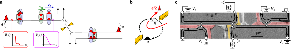
Figure 1: Experimental setup. a, In the presence of two strongly coupled quantum Hall channels at $\nu=2$, tunneling electrons $e$ (individual red wave-packets) progressively split into two pairs (circled). The fast ‘charge’ pair (blue background) consists of two co-propagating $e/2$ wave-packets, one in each channel, whereas the slow ‘neutral’ pair (green background) consists of opposite $\pm e/2$ charges. The fractionalized $e/2$ charges propagate toward a central QPC (yellow split gates) of transmission $\tau_{\mathrm{c}}$, used to investigate their quantum statistics from the outgoing current cross-correlations. The strong coupling regime and the degree of fractionalization at the level of the central QPC are established separately through the evolution of the electron energy distribution function $f(\varepsilon)$ from a non-equilibrium double step (red inset) to a smoother function (magenta inset). b, Illustration of the time-braiding mechanism, whereby an impinging fractionalized $e/2$ charge (red) braids with an electron-hole pair (black) spontaneously excited at the central QPC. c, E-beam micrograph of the sample. The two copropagating edge channels are drawn as black lines with arrows indicating the chirality. The aluminum gates used to form the QPCs by field effect are highlighted in false colors (sources in red, central analyzer in yellow). A negative voltage is applied to the non-colored gates to reflect the edge channels at all times. Tunneling at the sources is controlled by the applied dc voltages $V_{\mathrm{1,2,3,4}}$ and through their gate-controlled transmission probability $\tau_{\mathrm{s}}$.

Anyonic exchange statistics can be revealed via interferometry, whereby anyons along the edge move around those in the bulk, and acquire a braiding (double exchange) phase ^{6, 9, 10, 11}. An alternative probe, not requiring involved heterostructures with built-in screening, is provided by a mixing process at an ‘analyzer’ quantum point contact (QPC) ¹². If the impinging quasiparticle beams are dilute (Poissonian), the outgoing current cross-correlations carry a signature of anyonic statistics ^{12, 13, 14}. These dilute beams are created upstream by sources typically realized by voltage-biased QPCs set in the tunneling regime. The signature of anyonic statistics becomes particularly straightforward with two symmetric sources, a configuration often referred to as a ‘collider’ ¹⁴. In this simple case, the cross-correlations for free fermions vanish, whereas a negative signal is considered to be a strong marker of anyonic statistics^{14, 6, 15}. Such negative current cross-correlation signatures of anyons at filling factors $\nu=1/3$ and $2/5$ have recently been demonstrated ^{16, 17, 13, 18}.

However, FQH states present complications which impede the analysis and further manipulation of anyons: the edge structure is often undetermined between several alternatives ¹⁹, the tunneling density of states generally presents an anomalous voltage dependence ²⁰, and the decoherence along the edge appears to be very strong ^{11, 9, 10}. A promising alternative path is provided by the insight that fractional charges propagating along the edges of IQH states should also behave as fractional anyons ^{21, 22, 6}. Indeed, the exchange phase of two quasiparticles of charge $e^{*}$ propagating along an integer quantum Hall channel ²² is $\pi(e^{*}/e)^{2}$. This exchange phase can be linked to a dynamical Aharonov-Bohm effect ²⁴. In practice, such IQH fractional anyons could be obtained e.g. by driving the edge channel with a narrow voltage pulse, from the charge fractionalization across a Coulomb island, or by exploiting the intrinsic Coulomb coupling between co-propagating edge channels ^{25, 26, 22, 6}. The present work proposes and implements the latter strategy, and demonstrates the anyonic character of the resulting fractional charges from the emergence of negative cross-correlations.

We focus on the filling factor $\nu=2$, which has two copropagating edge channels and constitutes the most simple, canonical and robust IQH state with interacting channels. The edge physics is well described by a chiral Luttinger model involving two one-dimensional channels with a linear dispersion relation and short-range Coulomb interactions ^{27, 20, 28, 29, 30}. This theory, which has been successful in explaining many experimental findings such as multiple lobes in a Mach-Zehnder interferometer ^{31, 32, 33} or spin-charge separation ^{34, 35}, reformulates interacting fermionic edge states as two free edge magnetoplasmon (EMP) modes via bosonization. In the limit of weak inter-channel coupling, each EMP mode is localized in one different channel and the system can be mapped back into the free electron picture. In contrast, at strong coupling the two EMP modes are fully delocalized between the two quantum Hall channels and correspond to a charge mode, with identical charge density fluctuations on both channels, and a neutral mode, with opposite density fluctuations ^{36, 21, 26}. Experimentally, typical Al(Ga)As devices at $\nu=2$ often appear to be close to the strong coupling regime ^{37, 34, 35}.

Here we exploit such an inter-channel distribution of EMPs at strong coupling to split electrons into fractional charges. We start by injecting electrons into a single edge channel with a voltage-biased QPC. Then, downstream from the QPC, each injected electron progressively splits into two wave-packets. Assuming strong coupling, one is solely built upon charge EMPs propagating at velocity $v_{\mathrm{c}}$, and the other is constructed from neutral EMPs and has a slower velocity $v_{\mathrm{n}}$. If we consider separately the quantum Hall channel where the electron is injected, both wave-packets carry a fractional charge of $e/2$, whereas in the other channel they have opposite charges $\pm e/2$ (see Fig. 1a)^{26, 38}. Such fractional wave-packets propagate non-dispersively. Considered individually, they are predicted to behave as abelian anyons with non-trivial exchange phase ^{21, 6, 22, 6}.

To experimentally address the anyon character of fractional charges propagating along integer quantum Hall channels, we measure the current cross-correlations at the output of a ‘collider’ in the stationary regime (see Fig. 1a,c). As for the fractional quantum Hall version of the device¹⁴, direct anyon collisions are very rare and can be ignored in the relevant diluted beams limit^{15, 6}. The cross-correlation signal stems instead from a braiding in the time-domain between incident anyons and particle-hole pairs spontaneously excited at the QPC^{39, 12, 22, 15, 6, 13, 40, 41}, as illustrated in Fig. 1b. At integer filling factors, the pairs are always formed of fermionic particles (electrons and holes), whereas in the fractional quantum Hall regime they can consist of anyons. Therefore the time-braiding considered here takes place between two different types of quasiparticles, of fractional and integer charges. The braiding (double exchange) phase $2\theta$ acquired in such heterogeneous cases characterizes the so-called mutual quantum statistics. It is predicted to take the fractional value of $2\theta=\pi$ (compared to $0\,(\mathrm{mod}\,2\pi)$ for the braiding of fermions or bosons). Note that while the braiding mechanism is equally relevant for a single incident beam of fractional quasiparticles or for two symmetric beams, the latter ‘collider’ setup allows for a qualitative test of the unconventional anyon character from the mere emergence of non-zero cross-correlations at the output^{14, 15, 40, 41}.

Figure 2: Spectroscopy of the electron energy distribution $f(\varepsilon)$. The shape of $f(\varepsilon)$ reflects the inter-channel coupling regime and informs on the conditions for a complete charge fractionalization at the central QPC. One source is voltage biased at $V_{\mathrm{s}}$, here with $\tau_{\mathrm{s}}\approx 0.5$, and the same probe voltage $V_{\mathrm{p}}$ is applied across the other one (see schematic in a). Circles and triangles show data points with the voltage biased source QPC on the left and right side, respectively. Purple continuous lines and blue dashed lines represent exact theoretical predictions in the strong coupling regime for a time delay between charge and neutral pairs of $\delta t=$ $64\text{\,}\mathrm{p}\mathrm{s}$ and $\infty$, respectively (see Supplementary Information). Insets: Cross-correlations $S_{12}$ versus probe voltage $V_{\mathrm{p}}$. Main panels: $f(\varepsilon)$ obtained by differentiation of $S_{12}$, see Eq. (1) with $\tau_{\mathrm{c}}\simeq 0.5$. a,b,c: Data and theory at $T\simeq$$11\text{\,}\mathrm{m}\mathrm{K}$ for a source voltage $V_{\mathrm{s}}=\,$$23\text{\,}\mathrm{\SIUnitSymbolMicro V}$, $35\text{\,}\mathrm{\SIUnitSymbolMicro V}$, and $70\text{\,}\mathrm{\SIUnitSymbolMicro V}$, respectively.

The sample, shown in Fig. 1c, is nanostructured from an Al(Ga)As heterostructure and measured at $11\text{\,}\mathrm{m}\mathrm{K}$ and $5.2\text{\,}\mathrm{T}$. It consists of two source QPCs (metallic split gates colored red) located at a nominal distance $d=$ $3.1\text{\,}\mathrm{\SIUnitSymbolMicro m}$ from the central ‘analyzer’ QPC (yellow gates). If not stated otherwise, all QPCs are set to partially (fully) reflect the outer (inner) edge channel, and the analyzer QPC is tuned to an outer edge channel transmission probability $\tau_{\mathrm{c}}\simeq 0.5$. A negative voltage is also applied to the non-colored gates to reflect the edge channels at all times, as schematically depicted. Low-frequency current auto-correlations $\langle\delta I_{1}^{2}\rangle$ and $\langle\delta I_{2}^{2}\rangle$ on the left and right side, respectively, and cross-correlations $\langle\delta I_{1}\delta I_{2}\rangle$ across the analyzer QPC are measured simultaneously. In the following, the excess noises are denoted $S_{ij}\equiv\langle\delta I_{i}\delta I_{j}\rangle-\langle\delta I_{i}\delta I_{j}\rangle(V_{1,2,3,4}=0)$ with $i,j\in\{1,2\}$.

Electron fractionalization

First we need to ensure that the device is in the strong coupling regime, and to determine under which conditions the tunneling electrons are fractionalized into well-separated $e/2$ charges at the analyzer QPC.

Our straightforward approach is to inject energy into one edge channel at a source, and to probe the energy redistribution at the analyzer ⁴². Indeed, the fractionalization of the tunneling electron coincides with the emergence of charge pulses in the other, co-propagating edge channel and, consequently, with a transfer of energy. Furthermore, the full EMP delocalization between both channels, which is specific to the strong coupling limit, also translates into an equal redistribution of energy between the channels at long distances⁴³.

In this measurement, only one source QPC is used together with the analyzer. We inject energy into the outer channel by applying a constant dc voltage bias $V_{\mathrm{s}}$ across the source QPC (e.g., $V_{1}=V_{\mathrm{s}}/2$ and $V_{3}=-V_{\mathrm{s}}/2$ for the left source, Fig. 1c). The resulting electron energy distribution immediately downstream of the injection point $f_{\mathrm{inj}}$ takes the shape of a double step (red inset in Fig. 1a), where $f_{\mathrm{inj}}(\varepsilon)=\tau_{\mathrm{s}}f_{\mathrm{FD}}(\varepsilon+eV_{\mathrm{s}}/2)+(1-\tau_{\mathrm{s}})f_{\mathrm{FD}}(\varepsilon-eV_{\mathrm{s}}/2)$, with $\tau_{\mathrm{s}}$ the transmission probability of outer channel electrons across the source QPC, and $f_{\mathrm{FD}}$ the Fermi-Dirac distribution.

The electron energy distribution spectroscopy at the analyzer is performed in the out-of-equilibrium outer edge channel by measuring the cross-correlations $S_{12}$ vs the probe voltage $V_{\mathrm{p}}$ that controls the electrochemical potential of the equilibrium edge channel on the other side (e.g., $V_{2}=V_{4}=V_{\mathrm{p}}$). The latter’s cold Fermi distribution acts as a step filter^{44, 45, 46}, up to a $k_{\mathrm{B}}T\approx$ 0.1 µeV rounding. The probed out-of-equilibrium electron energy distributions $f$ displayed in Fig. 2 are computed from the measured $S_{12}$ (inset) using ^{47, 44}:

$$f(\varepsilon=eV_{\mathrm{p}})\equiv\frac{1}{2}\left(1+\frac{h}{2e^{2}\;\tau_{\mathrm{c}}(1-\tau_{\mathrm{c}})}\frac{\partial S_{12}(V_{\mathrm{p}})}{e\partial V_{\mathrm{p}}}\right).$$ (1)

The three panels in Fig. 2 show the evolution of $f$ with the source bias voltage $V_{\mathrm{s}}$, at $\tau_{\mathrm{s}}\simeq\tau_{\mathrm{c}}\simeq 0.5$. Whereas at low $V_{\mathrm{s}}=$ $23\text{\,}\mathrm{\SIUnitSymbolMicro V}$ (a) $f$ remains close to a double-step function, we observe a marked relaxation towards an intermediate shape at $V_{\mathrm{s}}=$ $35\text{\,}\mathrm{\SIUnitSymbolMicro V}$ (b) and, at high bias $V_{\mathrm{s}}=$ $70\text{\,}\mathrm{\SIUnitSymbolMicro V}$ (c), $f$ takes the shape of a broad single step closely matching the long distance prediction for the strong coupling limit (blue dashed lines). This last observation establishes that the present device is in the strong coupling limit. Furthermore, since only the data for $70\text{\,}\mathrm{\SIUnitSymbolMicro V}$ agrees well with the long distance prediction, this indicates that the fractionalized $e/2$ wave-packets become well-separated at the analyzer for a bias $V_{\mathrm{s}}$ between $35\text{\,}\mathrm{\SIUnitSymbolMicro V}$ and $70\text{\,}\mathrm{\SIUnitSymbolMicro V}$. In that case, the wave-packet time-width $h/eV_{\mathrm{s}}$⁴⁸ is smaller than the time delay between the arrival of fractionalized $e/2$ charges at the analyzer QPC $\delta t=d/v_{\mathrm{n}}-d/v_{\mathrm{c}}$.

Further evidence of the good theoretical description of the device is provided by the quality of the quantitative comparison between the data and the exact calculations of $f$ at finite distance (purple continuous lines). These predictions were obtained by an extension of the theory involving a subsequent refermionization of the bosonized Hamiltonian, which enables a full access to the cross-correlations and out-of-equilibrium electron distributions (see Supplementary Information). The only fitting parameter is the time delay $\delta t$. Here it is fixed to $\delta t=$ $64\text{\,}\mathrm{p}\mathrm{s}$, and its associated effective velocity $d/\delta t=$ $5\text{\times}{10}^{4}\text{\,}\mathrm{m}\leavevmode\nobreak\ \mathrm{s}^{-1}$ is comparable to EMP velocity measurements in similar samples³⁵. See also Extended Data Fig. 1 for a comparison at additional intermediate voltages, Extended Data Fig. 2 for measurements with a dilute quasiparticle beam, and Extended Data Fig. 3 for a (less-controlled) power injection in the inner edge channel.

Negative cross-correlation signature of anyon statistics

We now turn to the cross-correlation investigation of the fractional mutual braiding statistics between $e/2$ edge quasiparticles and electrons. Figure 3 displays the central measurement of cross-correlations in the configuration of two sources injecting symmetric dilute beams toward the analyzer. The source QPCs are biased at a voltage $V_{\mathrm{s}}$ equally distributed on the two inputs ($V_{1,2}=-V_{3,4}=V_{\mathrm{s}}/2$, Fig. 1c), and set to a transmission $\tau_{\mathrm{s}}\approx 0.05$ (top inset in Fig. 3).

The relevant parameter to investigate the cross-correlation signature of anyonic statistics is the generalized Fano factor ¹⁴

$$P\equiv\frac{S_{\mathrm{12}}}{\tau_{\mathrm{c}}(1-\tau_{\mathrm{c}})S_{\mathrm{\Sigma}}},$$ (2)

where $\tau_{\mathrm{c}}$ is the analyzer transmission, and $S_{\mathrm{\Sigma}}$ is the sum of the current noises emitted from the two source QPCs. $P$ carries information on the braiding statistics, with a high bias voltage limit that depends on the braiding phase ^{14, 41, 40}. If the (mutual) braiding statistics of free quasiparticles is trivial, such as for fermions or bosons, then $P$ is zero, whereas it is non-zero otherwise. The mere observation of a non-zero $P$ therefore provides a qualitative signature of an unconventional braiding statistics. However, we stress the importance of unambiguously establishing the underlying theoretical description of the system. For instance, negative cross-correlations could also be obtained with fermions, by phenomenologically introducing a redistribution of energy (see Supplementary Information). Here we have ascertained the suitability of the fractional charge picture through electron energy distribution spectroscopy. In practice, $P$ is extracted from the slope of $S_{\mathrm{12}}/(\tau_{\mathrm{c}}(1-\tau_{\mathrm{c}}))$ vs $S_{\mathrm{\Sigma}}$, as shown in Fig. 3 (green dashed line). Note that the measurements of $S_{\mathrm{\Sigma}}$ and $S_{\mathrm{12}}$ are performed simultaneously, by exploiting the current conservation relation $S_{\mathrm{\Sigma}}=S_{11}+S_{22}+2S_{12}$.

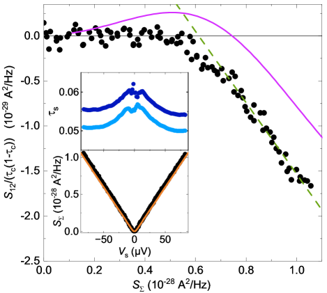
Figure 3: Cross-correlation signature of fractional statistics with symmetric dilute beams. Measured excess shot noise $S_{\mathrm{12}}/(\tau_{\mathrm{c}}(1-\tau_{\mathrm{c}}))$ as a function of source shot noise $S_{\mathrm{\Sigma}}$ for a small source QPC transmission $\tau_{\mathrm{s}}=0.05$. The purple continuous line displays the strong inter-channel coupling prediction for $\delta t=$ $64\text{\,}\mathrm{p}\mathrm{s}$. The dashed green line denotes the slope, i.e., the Fano factor (see Main text), yielding $P\simeq-0.38$. Top inset: Measured left/right source QPC dc transmission as a function of bias voltage, shown in light/dark blue, respectively. Bottom inset: Sum of sources’ shot noise $S_{\mathrm{\Sigma}}$ vs source bias voltage $V_{\mathrm{s}}$. The orange line displays Eq. (3) with $T=$ $11\text{\,}\mathrm{m}\mathrm{K}$, the independently measured temperature.

Figure 4: Cross-correlations vs dilution of symmetric beams. Main panels and insets show, respectively, the generalized Fano factor $P$ and the renormalized cross-correlations $S_{\mathrm{12}}(V_{\mathrm{s}}=$$70\text{\,}\mathrm{\SIUnitSymbolMicro V}$$)/(\tau_{\mathrm{c}}(1-\tau_{\mathrm{c}}))$ vs the outer edge channel transmission $\tau_{\mathrm{s}}$ of the symmetric source QPCs. Symbols are data points. Blue lines are high bias/long $\delta t$ predictions. Purple lines are $S_{\mathrm{12}}(V_{\mathrm{s}}=$$70\text{\,}\mathrm{\SIUnitSymbolMicro V}$$)/(\tau_{\mathrm{c}}(1-\tau_{\mathrm{c}}))$ predictions at $\delta t=$ $64\text{\,}\mathrm{p}\mathrm{s}$. a, The cross-correlation signal and corresponding $P_{\mathrm{outer}}$ (open circles) are measured by partially transmitting at the central QPC ($\tau_{\mathrm{c}}\approx 0.5$) the same outer edge channel (black) where electrons are tunneling at the sources (see schematics). This is the standard ‘collider’ configuration. b, The cross-correlation signal and corresponding $P_{\mathrm{inner}}$ are obtained by setting the central QPC to partially transmit ($\tau_{\mathrm{c}}\approx 0.5$) the inner edge channel (grey), whereas electrons are tunneling into the outer edge channel at the sources (see schematic). In this particular configuration, the source shot noise does not directly contribute to the cross-correlation signal. Filled symbols in the main panel display $P_{\mathrm{outer}}-1$, with $P_{\mathrm{outer}}$ the data in (a) and $-1$ corresponding to the subtraction of the source shot noise.

We first check that $S_{\mathrm{\Sigma}}$ reflects the charge $e$ of injected electrons (Fig. 3, bottom inset). This is attested by the good quantitative agreement, without any fit parameter, between the data (symbols) and the shot noise prediction for electrons (line) given by⁴⁷:

$$S_{\mathrm{\Sigma}}=2\frac{e^{2}}{h}\!\!\sum_{i=L,R}\!\!\tau_{\mathrm{i}}(1-\tau_{\mathrm{i}})eV_{\mathrm{s}}\!\left[\coth\!\left(\frac{eV_{\mathrm{s}}}{2k_{\mathrm{B}}T}\right)-\frac{2k_{\mathrm{B}}T}{eV_{\mathrm{s}}}\right]\!\!,$$ (3)

with $T=$ $11\text{\,}\mathrm{m}\mathrm{K}$ and $\tau_{\mathrm{L(R)}}$ the measured dc transmission of the left (right) source shown in the top inset.

We then focus on the cross-correlation investigation of anyonic behavior. As shown in Fig. 3, $S_{12}\approx 0$ at low bias, up to $S_{\Sigma}\approx$ $6\text{\times}{10}^{-29}\text{\,}\mathrm{A}^{2}\leavevmode\nobreak\ \mathrm{H}\mathrm{z}^{-1}$ corresponding to $|V_{\mathrm{s}}|\approx$ $45\text{\,}\mathrm{\SIUnitSymbolMicro V}$. This $P\approx 0$ signals a trivial mutual statistics, which is expected in the low bias regime where the injected electron is not fractionalized at the analyzer. Then, at $|V_{\mathrm{s}}|\gtrsim$ $45\text{\,}\mathrm{\SIUnitSymbolMicro V}$ where the fractionalization takes place according to $f(\varepsilon)$ spectroscopy, $S_{12}$ turns negative with a slope of $P\simeq-0.38$ (green dashed line). The clear negative signal with a fixed slope constitutes a strong qualitative marker of non-trivial mutual braiding statistics, as further discussed below.

The relationship between negative cross-correlations and anyonic mutual statistics in the dilute limit of small $\tau_{\mathrm{s}}$ (or, symmetrically, small $1-\tau_{s}$) is most clearly established in a perturbative analysis along the lines of Morel et al⁶. For $\tau_{\mathrm{s}}\ll 1$ and at long distances from the source, we find (see Supplementary Information):

$$P\simeq\frac{\sin^{2}\theta}{\theta^{2}}\ln{\tau_{\mathrm{s}}},$$ (4)

with $2\theta$ the mutual braiding (double exchange) phase. For quasiparticles of charges $q$ and $q^{\prime}$ along an integer quantum Hall channel, theory predicts $\theta=\pi qq^{\prime}/e^{2}$ (see, e.g., Ref. 22). In the present case of a braiding between incident fractional charges $e/2$ and spontaneously generated electron-hole pairs, we thus have $\theta=\pi/2$ and $P\simeq\frac{4}{\pi^{2}}\ln{\tau_{\mathrm{s}}}$ (see also Ref. 28 for the same prediction, but without the explicit connection to the fractional mutual statistics). Note that in the present integer quantum Hall implementation, the relationship between $P$ and $\theta$ is not complicated by additional parameters, such as the fractional quasiparticles’ scaling dimension and topological spin that both come into play in the fractional quantum Hall regime^{14, 15, 40, 41}. However, achieving $P\propto\ln\tau_{\mathrm{s}}$ requires large $|\ln\tau_{\mathrm{s}}|$ and thus exponentially small $\tau_{\mathrm{s}}$, which complicates a quantitative comparison of experimental data with Eq. (4). Accordingly, injecting $\tau_{\mathrm{s}}=0.05$ ($\ln\tau_{\mathrm{s}}\simeq-3$) into Eq. (4) gives a slope $P\simeq-1.2$, substantially more negative than the observations.

A better data-theory agreement can be obtained with a non-perturbative treatment of the sources. Indeed, the predicted slope in the high bias/long distance limit at $\tau_{\mathrm{s}}=0.05$ is $P\simeq-0.35$ (see Eq. (54) in Supplementary Information), close to the observed $P\simeq-0.38$. The full finite bias/finite distance prediction (purple continuous line in Fig. 3) also reproduces the overall shape of the measurements, although with a noticeable horizontal shift (see Supplementary Information for a discussion of possible theoretical limitations). Further evidence of the underlying anyonic mechanism is provided from the effect of the dilution of the quasiparticle beam.

Cross-correlations vs beam dilution

Here we explore the effect of dilution by sweeping the transmission across the two symmetric sources over the full range $\tau_{\mathrm{s}}\in[0,1]$, and we also extend our investigation to the inner edge channel where the electron fractionalization results in two pulses carrying opposite charges $\pm e/2$ (see Fig. 1a).

Let us first consider the previous/standard configuration, with source QPCs and analyzer QPC set to partially transmit the same, outer, channel. Away from the dilute limits, $P$ and $S_{\mathrm{12}}$ show a change of sign (see Fig. 4a). This results from an increasing importance of the positive contribution from the noise generated at the sources ⁴⁹ with respect to the noise generated at the analyzer involving the emergence of mechanisms other than time braiding (such as collisions) ^{6, 40}. In addition we see that the data are symmetric around $\tau_{\mathrm{s}}=0.5$, due to the unchanging electron nature of tunneling particles into the IQH edges (with small deviations possibly from inter-channel tunneling, see Supplementary Information). This is in contrast with the fractional quantum Hall regime where the nature of the tunneling quasiparticles changes ⁵⁰ between $\tau_{\mathrm{s}}\ll 1$ and $1-\tau_{\mathrm{s}}\ll 1$. The agreement with theory observed for $P(\tau_{\mathrm{s}})$, and more specifically for the $\tau_{\mathrm{s}}$ dependence in the dilute limits $\tau_{\mathrm{s}}\ll 1$ and $1-\tau_{\mathrm{s}}\ll 1$, further establishes the experimental cross-correlation signature of fractional mutual statistics. Note that the less precise agreement on the full $S_{12}$ signal is reminiscent of the horizontal shift of the negative slope in Fig. 3.

We then consider in Fig. 4b the alternative configuration, where the analyzer is set to $\tau_{\mathrm{c}}\simeq 0.5$ for the inner edge channel (the outer edge channel, where electrons are injected at the sources, being fully transmitted, see schematics). In that case, the cross-correlation signal is always negative due to charge conservation. The positive contribution $\tau_{\mathrm{c}}(1-\tau_{\mathrm{c}})S_{\Sigma}$ from the partition of the current noise generated at the sources is absent since the electron tunneling at the sources does not take place in the probed inner edge channel. In the strong coupling limit where fractional charges of identical amplitude $e/2$ propagate on both inner and outer channel, the same unconventional braiding is expected to have the same cross-correlation consequences. The absence of source noise then simply results in an offset: $P_{\mathrm{inner}}=P_{\mathrm{outer}}-1$ ($S_{12}^{\mathrm{inner}}=S_{12}^{\mathrm{outer}}-\tau_{\mathrm{c}}(1-\tau_{\mathrm{c}})S_{\Sigma}$), where the label inner/outer indicates the channel probed at the analyzer. For a direct comparison, $P_{\mathrm{outer}}-1$ is also shown (filled stars). The agreement between the two data sets provides an additional, direct confirmation that the device is in the strong coupling regime. It also experimentally establishes the robust contribution from the source noise to $S_{12}$, allowing to distinguish it from the effect of time-braiding.

Summary and outlook

QPCs used as electron sources have been combined with the intrinsic Coulomb interaction between co-propagating integer quantum Hall channels to form dilute beams of fractional charges behaving as anyons. Their fractional quantum statistics was established by the emergence of negative current cross-correlations between the two outputs of a downstream analyzer QPC, similarly to previous observations in the fractional quantum Hall regime. By contrast, when applying sufficiently low source bias voltages such that the tunneling electrons are preserved (not fractionalized), the absence of a cross-correlation signal coincides with their fermion character.

We believe that the demonstrated integer quantum Hall platform opens a promising practical path to explore the emerging field of anyon quantum optics ⁵¹. Advanced and time-resolved quantum manipulations of anyons are made possible by the large quantum coherence along the integer quantum Hall edge and the robustness of the incompressible bulk. By tailoring single-quasiparticle wave-packets, for example with driven ohmic contacts, a vast range of fractional anyons of arbitrary exchange phase becomes available along the integer quantum Hall edges, well beyond the odd fractions of $\pi$ of Laughlin quasiparticles encountered in the fractional quantum Hall regime.

Methods

Sample fabrication
The device, shown in Fig. 1c of the Main text, is patterned in an AlGaAs/GaAs heterostructure forming a two-dimensional electron gas (2DEG) buried $95\text{\,}\mathrm{nm}$ below the surface. The 2DEG has a mobility of $2.5\text{\times}{10}^{6}\text{\,}{\mathrm{cm}}^{2}\text{\leavevmode\nobreak\ }{\mathrm{V}}^{-1}\text{\leavevmode\nobreak\ }{\mathrm{s}}^{-1}$ and a density of $2.5\text{\times}{10}^{11}\text{\,}{\mathrm{cm}}^{-2}$. It was nanofabricated following five standard e-beam lithography steps:

1. Ti-Au alignment marks are first deposited through a PMMA mask.

2. The mesa is defined by using a ma-N 2403 protection mask and by wet-etching the unprotected parts in a solution of H₃PO₄/H₂O₂/H₂O over a depth of $\sim$$100\text{\,}\mathrm{nm}$.

3. The ohmic contacts allowing an electrical connection with the buried 2DEG are realized by the successive depositions of Ni ($10\text{\,}\mathrm{nm}$) - Au ($10\text{\,}\mathrm{nm}$) - Ge ($90\text{\,}\mathrm{nm}$) - Ni ($20\text{\,}\mathrm{nm}$) - Au ($170\text{\,}\mathrm{nm}$) - Ni ($10\text{\,}\mathrm{nm}$) through a PMMA mask, followed by a 440°C annealing for $50\text{\,}\mathrm{s}$.

4. The split gates controlling the QPCs consist in $40\text{\,}\mathrm{nm}$ of aluminium deposited through a PMMA mask.

5. Finally, we deposit thick Cr-Au bonding ports and large-scale interconnects through a PMMA mask.

The nominal tip-to-tip distance of the Al split gates used to define the QPCs is $150\text{\,}\mathrm{nm}$.

Measurement setup
The sample is installed in a cryofree dilution refrigerator with important filtering and thermalization of the electrical lines, and immersed in a perpendicular magnetic field $B=$ $5.2\text{\,}\mathrm{T}$, which corresponds to the middle of the $\nu=2$ plateau. Cold $RC$ filters are mounted near the device: $200\text{\,}\mathrm{k\SIUnitSymbolOhm}$ - $100\text{\,}\mathrm{nF}$ on the lines controlling the split gates, $10\text{\,}\mathrm{k\SIUnitSymbolOhm}$ - $100\text{\,}\mathrm{nF}$ on the injection lines and $10\text{\,}\mathrm{k\SIUnitSymbolOhm}$ - $1\text{\,}\mathrm{nF}$ on the low frequency measurement lines.

Lock-in measurements are made at frequencies below $25\text{\,}\mathrm{Hz}$, using an ac modulation of rms amplitude below $k_{\mathrm{B}}T/e$. We calculate the dc currents and QPC transmissions by integrating the corresponding lock-in signal vs the source bias voltage (see the following and Ref. 52 for details).

The auto- and cross-correlations of the currents $I_{\mathrm{1}}$ and $I_{\mathrm{2}}$ (Fig. 1c) are measured with home-made cryogenic amplifiers ⁵³ around $0.86\text{\,}\mathrm{M}\mathrm{H}\mathrm{z}$, the resonant frequency of the two identical tank circuits along the two amplification chains. The measurements are performed by integrating the signal over the bandwidth of $[0.78,0.92]$ $\text{\,}\mathrm{M}\mathrm{H}\mathrm{z}$. The measurement setup is detailed in the supplemental material of Ref. 54.

Thermometry
The electron temperature in the sample is measured using the robust linear dependence of the thermal noise $S(T)\propto T$. At $T>$ $40\text{\,}\mathrm{mK}$, we use the (equilibrium) thermal noise plotted versus the temperature readout by the calibrated RuO₂ thermometer. The linearity is a confirmation of the electron thermalization and of the thermometer calibration. The quantitative value of the slope provides us with the gain of the full noise amplification chain, as detailed in the next section. To determine the temperature in the $T<$ $40\text{\,}\mathrm{mK}$ range, we measure the thermal noise and determine the corresponding temperature by linearly extrapolating from the $S(T>$ $40\text{\,}\mathrm{mK}$$)$ data. The values of $T$ obtained using the two amplification chains are found to be consistent. We also check that $T$ corresponds to the temperature obtained from standard shot noise measurements performed individually on each QPC ahead of and during each measurement. A $1\text{\,}\mathrm{mK}$ higher shot noise temperature is specifically associated with the top-right ohmic contact feeding the right source, and attributed to noise from the corresponding connecting line.

Calibration of the noise amplification chain
For each noise amplification chain $i\in\{1,2\}$, the gain factor $G^{\mathrm{eff}}_{\mathrm{i}}$ between current noise spectral density and raw measurements needs to be calibrated. From the slopes $s_{1}$ and $s_{2}$ of $S(T>$ $40\text{\,}\mathrm{mK}$$)$ measured, respectively, for the amplification chain 1 and 2 (see Thermometry), and the robust fluctuation-dissipation relation $S(T)=4k_{\mathrm{B}}T\,\mathrm{Re}[Z]$ with $Z$ the frequency dependent impedance of the tank circuit in parallel with the sample, we get:

$$G_{\mathrm{1(2)}}^{\mathrm{eff}}=\frac{s_{\mathrm{1(2)}}}{4k_{\mathrm{B}}(1/R_{\mathrm{tk}}^{\mathrm{1(2)}}+1/R_{\mathrm{H}})},$$ (5)

with $R_{\mathrm{H}}=h/2e^{2}$ the Hall resistance of the sample, and $R_{\mathrm{tk}}^{\mathrm{1(2)}}=$ $150\text{\,}\mathrm{k\SIUnitSymbolOhm}$ ($153\text{\,}\mathrm{k\SIUnitSymbolOhm}$) the separately obtained effective parallel resistance due to the dissipation in the tank circuit connected to the same port. With $G_{\mathrm{1}}^{\mathrm{eff}}$ and $G_{\mathrm{2}}^{\mathrm{eff}}$ given by the above relation, the gain for the cross-correlation signal reads $G_{\mathrm{12}}^{\mathrm{eff}}=\sqrt{G_{\mathrm{1}}^{\mathrm{eff}}G_{\mathrm{2}}^{\mathrm{eff}}}$ thanks to the good match of the two resonators. For more details see Ref. 52.

Differential (ac) and integral (dc) transmission

Source transmissions:

The transmissions of the left and right source QPC $\tau_{\mathrm{L,R}}$ are defined as the ratio between the dc current transmitted across the QPC

$$I_{\mathrm{L,R}}=\int_{0}^{V_{3,4}}\frac{\partial(I_{1}+I_{2})}{\partial V_{3,4}}dV_{3,4}$$ (6)

and the dc current $e^{2}V_{3,4}/h$ incident on one side of the QPC for the considered outer edge channel (i.e., half of the total injected current), yielding:

$$\tau_{\mathrm{L,R}}=\frac{2h}{e^{2}}\frac{I_{\mathrm{L,R}}}{V_{3,4}}.$$ (7)

In the specific case where the sources are set to partial transmission of the inner channel (case of Extended Data Fig. 3), source transmissions of the inner channel can similarly be defined as

$$\tau_{\mathrm{L,R}}^{\mathrm{\,\,\,\,\,\,\,\,in}}=\frac{2h}{e^{2}V_{1,2}}\int_{0}^{V_{1,2}}\left(\frac{e^{2}}{h}-\frac{\partial(I_{1}+I_{2})}{\partial V_{1,2}}\right)dV_{1,2}.$$ (8)

Analyzer transmission: Whereas above we use dc transmissions for the sources, in all measurements the relevant transmission of the analyzer is the ac transmission, obtained as

$$\tau_{\mathrm{c}}=\left.\left(\frac{\partial I_{2}}{\partial V_{3}}\right)\middle/\left(\frac{\partial(I_{1}+I_{2})}{\partial V_{3}}\right)\right..$$ (9)

In particular, there is no dc bias of the analyzer in the symmetric source configuration probing the quantum statistics.

Data availability
Plotted data, raw data, data analysis code and numerical code used to calculate the full theoretical predictions are available on Zenodo: https://zenodo.org/records/10492057.

Acknowledgments
We would like to thank P. Degiovanni and J.T. Chalker for discussions. This work was supported by the European Research Council (ERC-2020-SyG-951451), the French National Research Agency (ANR-16-CE30-0010-01 and ANR-18-CE47-0014-01), the French RENATECH network and DIM NANO-K. D.M. acknowledges support from Labex MME-DII grant ANR11-LBX-0023, and funding under The Paris Seine Initiative EMERGENCE programme 2019.

Author Contributions
P.G., C.P. and I.P. performed the experiment and analyzed the data with inputs from A.Aa., A.An., D.K. and F.P.; D.K. and C.M. developed the theory; D.K. wrote the code for numerical predictions; A.C. and U.G. grew the 2DEG; P.G and A.Aa. fabricated the sample with inputs from A.An.; Y.J. fabricated the HEMTs used in the cryogenic amplifiers for noise measurements; I.P. and P.G. wrote the manuscript with contributions from all authors; A.An. and F.P. led the project.

Competing interests
The authors declare no competing interests.

Additional Information
Correspondence and requests for materials should be addressed to I.P. and F.P.

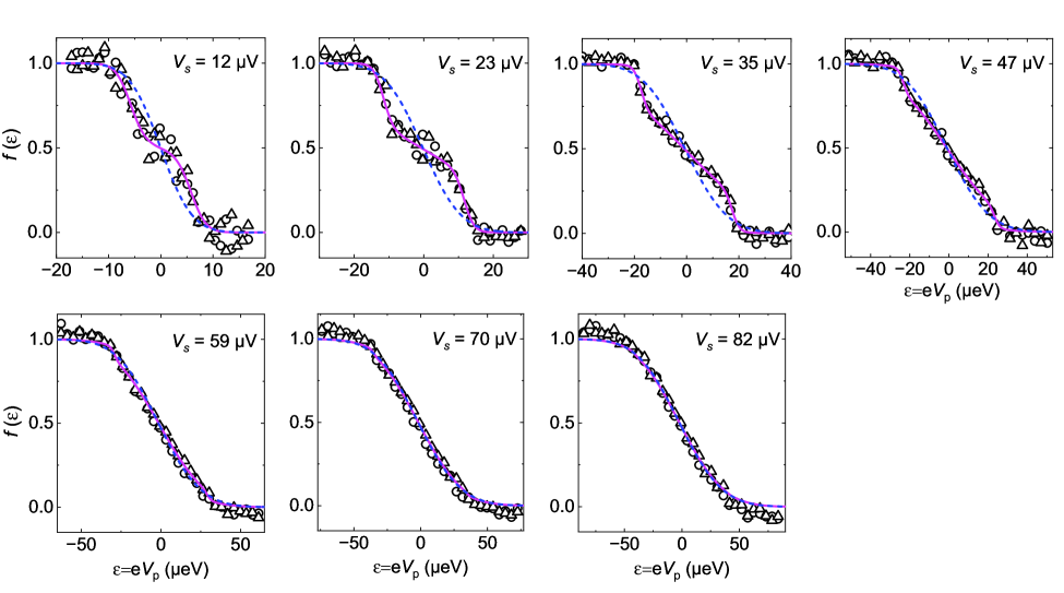
Extended Data Figure 1: Electron energy distribution spectroscopy at intermediate voltages. Electron energy distribution $f$ vs injected energy $\varepsilon$ for the source bias voltage $V_{\mathrm{s}}$ given in each panel, ranging from $12\text{\,}\mathrm{\SIUnitSymbolMicro V}$ to $82\text{\,}\mathrm{\SIUnitSymbolMicro V}$. The additional $V_{\mathrm{s}}$ complete the three values shown in Fig. 2. Squares and triangles correspond to $V_{\mathrm{s}}$ applied, respectively, to the left and right source QPC. Both source and analyzer transmissions are set to $0.5$. Continuous purple lines show the theoretical predictions for $\delta t=$ $64\text{\,}\mathrm{p}\mathrm{s}$ and the dashed blue lines those for $\delta t=\infty$.

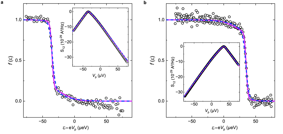
Extended Data Figure 2: Electron energy distribution spectroscopy at high beam dilution. Energy distribution $f$ obtained from $S_{12}$ (insets) by derivation, see Main text, Eq. (1). Panel a corresponds to $\tau_{\mathrm{s}}=$ 0.05 and panel b to $\tau_{\mathrm{s}}=$ 0.95. The analyzer transmission is set to $\tau_{\mathrm{c}}=0.5$ and bias voltage to $V_{\mathrm{s}}=$ $70\text{\,}\mathrm{\SIUnitSymbolMicro V}$. Injection is from the right QPC. Full purple and dashed blue line are the predictions for $\delta t=$ $64\text{\,}\mathrm{p}\mathrm{s}$ and $\delta t=\infty$ respectively.

Extended Data Figure 3: Electron energy distribution spectroscopy along the inner edge channel. a,b,c Energy distribution $f(\varepsilon)$ obtained by deriving the measured $S_{\mathrm{12}}$ (insets, see Eq. (1)) and plotted versus the probe energy $\varepsilon=eV_{\mathrm{p}}$, taken at bias voltage $V_{\mathrm{s}}=$ $23\text{\,}\mathrm{\SIUnitSymbolMicro V}$, $35\text{\,}\mathrm{\SIUnitSymbolMicro V}$ and $70\text{\,}\mathrm{\SIUnitSymbolMicro V}$ from left to right. The injection is on the inner channel and the measurement on the outer (see schematic in a). Circles and triangles correspond respectively to the injection from the left and right source. Both source and analyzer transmissions are tuned to $\tau_{\mathrm{s}}=\tau_{\mathrm{c}}=0.5$. Full purple and dashed blue line display the numerical predictions for $\delta t=$ $64\text{\,}\mathrm{p}\mathrm{s}$ and $\delta t=\infty$ respectively.

Extended Data Figure 4: Cross-correlations vs dilution at intermediate voltages and higher temperature. a, c, Cross-correlations $S_{12}/(\tau_{\mathrm{c}}(1-\tau_{\mathrm{c}}))$ as function of source QPC transmission $\tau_{\mathrm{s}}$ at $11\text{\,}\mathrm{m}\mathrm{K}$ (a,b) and $21\text{\,}\mathrm{m}\mathrm{K}$ (c, d). Extension of Fig. 4 from the Main text. Injection takes place in the external channel at all times, whereas the measurement is done on the external channel (a, c, e) or the internal channel (b, d, f). The solid lines in a-d are the prediction for $\delta t=$ $64\text{\,}\mathrm{p}\mathrm{s}$. Data at each bias voltage and their prediction have the same color (cf. legend). e, f, Fano factors extracted at $T=$ $21\text{\,}\mathrm{m}\mathrm{K}$ with the central QPC partially transmitting the outer (e) and inner (f) channel. Blue lines correspond to the high bias/large $\delta t$ prediction. Full stars in panel f display $P_{\mathrm{outer}}-1$.

Supplementary Information
for
Signature of anyonic statistics in the integer quantum Hall regime

I Non-perturbative theory

I.1 Introduction

In this Section we outline the theoretical description of the electron collider using a model which can be solved via refermionization techniques. We also present the results for the asymptotics of the noise in the small tunneling limit.

The notation in this section is different from the rest of the paper in order to keep the correspondence with previous work in Ref. 1 and in the upcoming theoretical publication.

The notation conversion is the following :

This section	Elsewhere
$T_{1}$	$\tau_{\mathrm{s}}$
$T_{2}$	$\tau_{\mathrm{s}}$
$T_{S}$	$\tau_{\mathrm{c}}$
bias $V$	bias $V_{\mathrm{s}}$
spin up ($\uparrow$) channel	inner channel
spin down ($\downarrow$) channel	outer channel
1’ channels (Fig. 5)	region biased by $V_{3}$ (Fig. 1c Main text)
2’ channels (Fig. 5)	region biased by $V_{1}$ (Fig. 1c Main text)
1 channels (Fig. 5)	region biased by $V_{2}$ (Fig. 1c Main text)
2 channels (Fig. 5)	region biased by $V_{4}$ (Fig. 1c Main text)

Table 1: Notation correspondence between this section and the rest of the paper.

The schematics of the model is shown in Fig. 5 for the noise measurement between channels $1_{\downarrow}$ and $2^{\prime}_{\downarrow}$. In the Main text this is outlined as the default configuration, i.e., injection and measurement in the outer channel. Other configurations can be calculated in a similar manner, and the theory will be detailed in an upcoming publication.

Let us consider a system with four edge states $1,1^{\prime},2,2^{\prime}$, each of which is carrying two co-propagating edge channels ($\uparrow,\downarrow$). The arrows denote the spin. The biasing scheme of biasing source QPCs with 0 and $eV$ in Fig. 5 is equivalent to biasing with $-eV/2$ and $+eV/2$ (used in the experiment) by gauge invariance.

Figure 5: Schematic of the model of the electron collider at $\nu=2$ with four chiral edge states (each carrying two edge channels). The channels $1^{\prime}_{\downarrow}$ and $2^{\prime}_{\downarrow}$ are coupled via a QPC positioned at $x=0$ with the tunneling probability $T_{2}$. Similarly the edge states $1_{\downarrow}$ and $2_{\downarrow}$ are coupled by another QPC with tunneling probability $T_{1}$. The channels $2^{\prime}_{\downarrow}$ and $1_{\downarrow}$ are further mixed by another QPC with tunneling probability $T_{s}$ positioned at $x=d$. The short-range interactions between the channels situated on the same edge are denoted by grey areas. The two top channels and the two bottom channels are biased with the chemical potentials $eV$ and the four channels in the middle are grounded. The current correlations are measured after the the QPC with the transmission $T_{s}$ between the channels $2^{\prime}_{\downarrow}$ and $1_{\downarrow}$. The model can be solved for other types of voltage/measurement configurations.

We model the non-interacting edge channels by the free-fermion Hamiltonian with linear dispersion (assuming the same Fermi-velocity $v_{F}$ in every channel). This is a standard description of edge states at integer filling factors. In addition, we assume that electrons on each edge interact via short-range interactions with strength $g$ which has the dimension of velocity. This model of interactions provides a good description of previous experiments at $\nu=2$ filling factor ^{2, 3, 1}. We note that in the experimental setup the long-range Coulomb interactions are expected to be screened by the metallic gates.

The QPCs 1,2 and S (see Fig. 5) are described using standard tunneling Hamiltonian with corresponding transmission amplitudes $v_{1},v_{2},v_{S}$, where the QPC S is positioned at distance $d$ from the QPCs 1,2. The Hamiltonian of the system shown in Fig. 5 reads

$$\hat{H}=-i\hbar v_{F}\sum_{\eta=1,1^{\prime},2,2^{\prime},s=\uparrow,\downarrow}\int_{-\infty}^{\infty}dx\ \hat{\Psi}^{\dagger}_{\eta s}(x)\partial_{x}\hat{\Psi}_{\eta s}(x)+2\pi\hbar g\sum_{\eta=1,1^{\prime},2,2^{\prime}}\int_{-\infty}^{\infty}\hat{\rho}_{\eta\uparrow}(x)\hat{\rho}_{\eta\downarrow}(x)dx\\ +[v_{1}\hat{\Psi}^{\dagger}_{1\downarrow}(0)\hat{\Psi}_{2\downarrow}(0)+v_{2}\hat{\Psi}^{\dagger}_{1^{\prime}\downarrow}(0)\hat{\Psi}_{2^{\prime}\downarrow}(0)+v_{s}\hat{\Psi}^{\dagger}_{2^{\prime}\downarrow}(d)\hat{\Psi}_{1\downarrow}(d)+h.c.].$$ (10)

Here $\hat{\Psi}_{\eta s}(x)$ are fermion annihilation operators on the corresponding edge channels, and $\hat{\rho}_{\eta s}(x)$ are fermion density operators. We use the same notation as in Ref. 4, which also presents the details of the refermionization approach, so we do not repeat these here. The noise between, e.g.,  channels $1_{\downarrow}$ and $2^{\prime}_{\downarrow}$ at position $x$ (see Fig.5) is defined in a standard way,

$$S_{1_{\downarrow}2^{\prime}_{\downarrow}}(V)=2\int_{-\infty}^{\infty}dt\ \langle\delta\hat{I}_{1_{\downarrow}}(x,t)\delta\hat{I}_{2^{\prime}_{\downarrow}}(x,0)\rangle,$$ (11)

and the operators $\delta\hat{I}_{\eta s}(x,t)$ are given in terms of the current operators $I^{H}_{\eta s}(x,t)$ in the Heisenberg representation,

$$\delta\hat{I}_{\eta s}(x,t)=\hat{I}^{H}_{\eta s}(x,t)-\langle\hat{I}^{H}_{\eta s}(x,t)\rangle.$$ (12)

The current operators in the interaction representation (where the tunneling plays the role of interactions) are given by the following expression

$$\hat{I}_{\eta s}(x,t)=-ev_{F}\hat{\rho}_{\eta s}(x,t).$$ (13)

It is worth citing the result for the noise obtained in this model in the non-interacting case $g=0$,

$$S^{(0)}_{1_{\downarrow}2^{\prime}_{\downarrow}}(V)=-2\left(\frac{e^{2}}{2\pi\hbar}\right)T_{s}R_{s}(T_{1}-T_{2})^{2}|eV|,$$ (14)

where $T_{1},T_{2},T_{S}$ are corresponding tunneling probabilities of the QPCs, which are related (in the non-interacting case) to the tunneling amplitudes as $T_{\alpha}=\sin^{2}(|\nu_{\alpha}|/\hbar v_{F})$. In the following we assume that these probabilities are known from the experiment. The voltage applied to the edge states is denoted as $V$. We note that the noise in the non-interacting case is always zero in the case of equal tunneling probabilities, $T_{1}=T_{2}$, and is independent of the distance $d$.

In the interacting case the model described by the Hamiltonian in Eq. (10) can be solved using the refermionization approach ⁴, as we describe below. Further details will be presented in the upcoming publication.

I.2 Bosonization

After introducing bosonic operators $\hat{\phi}_{\eta s}(x)$, Klein factors $\hat{F}_{\eta s}$, and number operators $\hat{N}_{\eta s}$ in the Schrödinger representation, as well as a short-distance cutoff, we can write the fermion operators in the bosonic form

$$\hat{\Psi}_{\eta s}(x)=(2\pi a)^{-1/2}\hat{F}_{\eta s}e^{i\frac{2\pi}{L}\hat{N}_{\eta s}x}e^{-i\hat{\phi}_{\eta s}(x)}.$$ (15)

The operators have the following commutation relations

$$[\hat{\phi}_{\eta s}(x),\partial_{y}\hat{\phi}_{\eta s}(y)]=-2\pi i\delta_{\eta\eta^{\prime}}\delta_{ss^{\prime}}\delta(x-y),\ \ \{\hat{F}_{\eta s}^{\dagger},\hat{F}_{\eta^{\prime}s^{\prime}}\}=2\delta_{\eta\eta^{\prime}}\delta_{ss^{\prime}},\text{ \ }[\hat{N}_{\eta s},\hat{F}_{\eta^{\prime}s^{\prime}}]=-\delta_{\eta\eta^{\prime}}\delta,$$ (16)

and the density operator is written in terms of the bosonic fields as

$$\hat{\rho}_{\eta s}(x)=\hat{N}_{\eta s}/L-(2\pi)^{-1}\partial_{x}\hat{\phi}_{\eta s}(x).$$ (17)

The Hamiltonian in Eq. (10) can be written in the bosonized form as

$$\hat{H}_{0}=\frac{\hbar v_{f}}{2}\sum_{\eta s}\int\frac{dx}{2\pi}[\partial_{x}\hat{\phi}_{\eta s}]^{2}+g\hbar\sum_{\eta}\int\frac{dx}{2\pi}\partial_{x}\hat{\phi}_{\eta\uparrow}\partial_{x}\hat{\phi}_{\eta\downarrow}+\frac{2\pi g\hbar}{L}\sum_{\eta}\hat{N}_{\eta\uparrow}\hat{N}_{\eta\downarrow}+\frac{2\pi}{L}\frac{\hbar v_{f}}{2}\sum_{\eta s}\hat{N}_{\eta s}(\hat{N}_{\eta s}+1)\\ +(2\pi a)^{-1}[v_{1}\hat{F}_{1\downarrow}^{\dagger}\hat{F}_{2\downarrow}e^{i[\hat{\phi}_{1\downarrow}(0)-\hat{\phi}_{2\downarrow}(0)]}+v_{2}\hat{F}_{1^{\prime}\downarrow}^{\dagger}\hat{F}_{2^{\prime}\downarrow}e^{i[\hat{\phi}_{1^{\prime}\downarrow}(0)-\hat{\phi}_{2^{\prime}\downarrow}(0)]}+v_{s}\hat{F}_{2^{\prime}\downarrow}^{\dagger}\hat{F}_{1\downarrow}e^{i[\hat{\phi}_{2^{\prime}\downarrow}(0)-\hat{\phi}_{1\downarrow}(0)]}+\mathrm{h.c.}].$$ (18)

I.3 Refermionization

We start with the refermionization of the four channels $(1_{\uparrow},1_{\downarrow},2^{\prime}_{\downarrow},2^{\prime}_{\uparrow})$. For these channels we can introduce new bosonic operators $\tilde{\chi}_{S+}(x),\tilde{\chi}_{A-}(x),\tilde{\chi}_{A+}(x),\tilde{\chi}_{S-}(x)$ (with $x$ the position counted from the last QPC $T_{s}$), which are related to the original bosonic operators $\phi_{1\uparrow}(x+d),\phi_{1\downarrow}(x+d),\phi_{2^{\prime}\downarrow}(x+d),\phi_{2^{\prime}\uparrow}(x+d)$ via the transformation $\tilde{\chi}^{T}=U\phi^{T}$, where on both sides we have vectors of operators $\tilde{\chi}(x)$ and $\phi(x+d)$, and $U$ is a $4\times 4$ matrix with constant coefficients, explicitly

$$U=\frac{1}{2}\left(\begin{array}[]{rrrr}1&1&1&1\\ 1&-1&1&-1\\ 1&1&-1&-1\\ 1&-1&-1&1\end{array}\right).$$ (19)

The dispersion of the bosons with $+$ index is given by the velocity $v_{+}=v_{F}+g$, and for $-$ index by the velocity $v_{-}=v_{F}-g$, where $g$ is the strength of the interactions.

We need to evaluate current correlation functions for the channels $1_{\downarrow}$ and $2^{\prime}_{\downarrow}$ at some position after the last QPC and at different times. For that we need to have expressions for the currents in these channels in terms of new fermions. The currents in terms of the original fermions can be obtained from the Heisenberg equations of motion for the density operators (in the interaction representation, where the tunneling is treated as interaction Hamiltonian, so the time evolution in this representation is given by the kinetic energy and the short-range interactions part), we have

$$\partial_{t}\hat{\rho}_{1\downarrow}(x,t)=-\partial_{x}(v_{F}\hat{\rho}_{1\downarrow}(x,t)+g\hat{\rho}_{1\uparrow}(x,t)),\ \ \partial_{t}\hat{\rho}_{2^{\prime}\downarrow}(x,t)=-\partial_{x}(v_{F}\hat{\rho}_{2^{\prime}\downarrow}(x,t)+g\hat{\rho}_{2^{\prime}\uparrow}(x,t)),$$ (20)

so that the corresponding currents are given in terms of original fermions in the interaction representation as

$$\hat{I}_{1\downarrow}(x,t)=-e(v_{F}\hat{\rho}_{1\downarrow}(x,t)+g\hat{\rho}_{1\uparrow}(x,t)),\ \ \hat{I}_{2^{\prime}\downarrow}(x,t)=-e(v_{F}\hat{\rho}_{2^{\prime}\downarrow}(x,t)+g\hat{\rho}_{2^{\prime}\uparrow}(x,t)).$$ (21)

The density operators can be expressed in terms of bosonic fields as

$$\hat{\rho}_{\eta s}(x,t)=\hat{N}_{\eta s}(t)/L-\frac{1}{2\pi}\partial_{x}\hat{\phi}_{\eta s}(x,t),$$ (22)

where $\hat{N}_{\eta s}/L$ are the fermion number operators, and $L$ is the system length. In the following we will omit the number operators to simplify the notations because they transform in the same way as the fields under linear transformation with the matrix $U$. We will restore them at the end.

Using the inverse transformation with the matrix $U^{-1}$ ($U^{-1}=U$), we can write the currents at position $d$ in terms of transformed density operators (which are related to $\tilde{\chi}$ fields via equation similar to Eq.(22)),

$$\hat{I}_{1\downarrow}(d,t)=-e\frac{1}{2}[v_{+}(\tilde{\rho}_{S+}(0,t)+\tilde{\rho}_{A+}(d,t))-v_{-}(\tilde{\rho}_{A-}(0,t)+\tilde{\rho}_{S-}(0,t))],$$ (23)

$$\hat{I}_{2^{\prime}\downarrow}(d,t)=-e\frac{1}{2}[v_{+}(\tilde{\rho}_{S+}(0,t)-\tilde{\rho}_{A+}(0,t))+v_{-}(\hat{\rho}_{A-}(0,t)-\tilde{\rho}_{S-}(0,t))].$$ (24)

We can rewrite these expressions in a more convenient form

$$\hat{I}_{1\downarrow}(d,t)=\frac{e}{2}(\hat{I}_{0}(d,t)+\hat{I}_{1}(d,t)),\ \ \hat{I}_{2^{\prime}\downarrow}=\frac{e}{2}(\hat{I}_{0}(d,t)-\hat{I}_{1}(d,t)),$$ (25)

where we defined

$$\hat{I}_{0}(d,t)\equiv-v_{+}\tilde{\rho}_{S+}(+0,t)+v_{-}\tilde{\rho}_{S-}(+0,t),\ \ \hat{I}_{1}(d,t)\equiv-v_{+}\tilde{\rho}_{A+}(+0,t)+v_{-}\tilde{\rho}_{A-}(+0,t).$$ (26)

We can now proceed with calculations of the noise, where we need the following correlator

$$\langle\hat{I}_{1\downarrow}(d,t_{1})\hat{I}_{2^{\prime}\downarrow}(d,t_{2})\rangle=\langle\hat{I}_{0}(d,t_{1})\hat{I}_{0}(d,t_{2})\rangle-\langle\hat{I}_{1}(d,t_{1})\hat{I}_{1}(d,t_{2})\rangle-\langle\hat{I}_{0}(d,t_{1})\hat{I}_{1}(d,t_{2})\rangle+\langle\hat{I}_{1}(d,t_{1})\hat{I}_{0}(d,t_{2})\rangle.$$ (27)

After refermionization one can write the Hamiltonian for the four channels coupled by a QPC $T_{s}$ in terms of free fermions with the standard tunneling term $H^{ref}_{T_{s}}=\tilde{v}_{s}\tilde{\Psi}^{\dagger}_{A_{+}}(0)\tilde{\Psi}_{A_{-}}(0)+h.c.$ with $\tilde{v}_{s}$ being renormalised tunneling strength ⁴. Below we will take this as the actual tunneling strength (e.g. the one which is measured in experiments) and denote the tunneling and reflection amplitudes as $t_{s},r_{s}$. We note that the refermionized tunneling operator does not affect the fields with indices $S_{+},S_{-}$. The fermion operators $\tilde{\Psi}_{A_{+}}$ and $\tilde{\Psi}_{A_{-}}$ are transformed by the last QPC in the usual way,

$$\tilde{\Psi}_{A_{+}}(+0,t)=r_{s}\tilde{\Psi}_{A_{+}}(-0,t)-it_{s}\tilde{\Psi}_{A_{-}}(-0,t),$$ (28)

$$\tilde{\Psi}_{A_{-}}(+0,t)=-it_{s}\tilde{\Psi}_{A_{+}}(-0,t)+r_{s}\tilde{\Psi}_{A_{+}}(-0,t),$$ (29)

where $+0$ and $-0$ are the positions just after and just before the QPC $T_{s}$ correspondingly.

Because the operator $\hat{I}_{0}$ does not transform under the action of the tunneling Hamiltonian $H^{ref}_{T_{s}}$ we can write the current $\hat{I}_{0}$ in terms of original fermion densities

$$\hat{I}_{0}(d,t)=-v_{+}\tilde{\rho}_{S+}(0,t)+v_{-}\tilde{\rho}_{S-}(0,t)=-\frac{v_{+}}{2}(\hat{\phi}_{1\uparrow}(d,t)+\hat{\phi}_{1\downarrow}(d,t)+\hat{\phi}_{2^{\prime}\downarrow}(d,t)+\hat{\phi}_{2^{\prime}\uparrow}(d,t))\\ +\frac{v_{-}}{2}(\hat{\phi}_{1\uparrow}(d,t)-\hat{\phi}_{1\downarrow}(d,t)-\hat{\phi}_{2^{\prime}\downarrow}(d,t)+\hat{\phi}_{2^{\prime}\uparrow}(d,t)).$$ (30)

We note that the operators on the right hand side are given in the Heisenberg representation with the Hamiltonian including interactions and the tunneling at both QPC 1 and QPC 2.

Now we need to refermionize the subsystems connected by the first two QPCs (e.g. we refermionize separately channels with primed indices, and channels with unprimed indices). In order to do that we introduce operators $\hat{\chi}(x)$ related to transformations of the bottom four channels and operators $\hat{\chi}^{\prime}(x)$ related to top four channels

$$(\hat{\chi}_{S+}(x),\hat{\chi}_{A-}(x),\hat{\chi}_{A+}(x),\hat{\chi}_{S-}(x))^{T} =U(\hat{\phi}_{1\uparrow}(x),\hat{\phi}_{1\downarrow}(x),\hat{\phi}_{2\downarrow}(x),\hat{\phi}_{2\uparrow}(x))^{T}$$ (31)

$$(\hat{\chi}^{\prime}_{S+}(x),\hat{\chi}^{\prime}_{A-}(x),\hat{\chi}^{\prime}_{A+}(x),\hat{\chi}^{\prime}_{S-}(x))^{T} =U(\hat{\phi}_{1^{\prime}\uparrow}(x),\hat{\phi}_{1^{\prime}\downarrow}(x),\hat{\phi}_{2^{\prime}\downarrow}(x),\hat{\phi}_{2^{\prime}\uparrow}(x))^{T}.$$ (32)

Using these transformation we can represent the current operator $\hat{I}_{0}(d,t)$ in terms of the $\hat{\chi}$ and $\hat{\chi}^{\prime}$ operators,

$$\hat{I}_{0}(d,t)=-\frac{v_{+}}{2}(\hat{\rho}_{S_{+}}(d,t)+\hat{\rho}_{A_{+}}(d,t)+\hat{\rho}^{\prime}_{S_{+}}(d,t)-\hat{\rho}^{\prime}_{A_{+}}(d,t))+\frac{v_{-}}{2}(\hat{\rho}_{A_{-}}(d,t)+\hat{\rho}_{S_{-}}(d,t)-\hat{\rho}^{\prime}_{A_{-}}(d,t)+\hat{\rho}^{\prime}_{S_{-}}(d,t)).$$ (33)

We note that there is no coherence between primed and unprimed terms as well as between $S+,S-$ terms because they are not connected by refermionized QPCs 1 and 2, as before (only $A_{+},A_{-}$ and $A^{\prime}_{+},A^{\prime}_{-}$ channels are connected by QPC 1 and QPC 2 correspondingly).

We need to relate the operators in the current (taken after QPCs 1 and 2) to the operators before these QPCs.

$$\hat{\Psi}^{\dagger}_{A_{-}}(+0,\tau)\hat{\Psi}_{A_{-}}(+0,\tau)=(+it_{1}\hat{\Psi}^{\dagger}_{A_{+}}(-0,\tau)+r_{1}\hat{\Psi}^{\dagger}_{A_{-}}(-0,\tau))(-it_{1}\hat{\Psi}_{A_{+}}(-0,\tau)+r_{1}\hat{\Psi}_{A_{-}}(-0,\tau)),$$ (34)

and similarly for the transformation of $A+$ operators.

We can now use these transformations to write the current correlators (noting that the $A_{+}$ and $A_{-}$ operators on the r.h.s. are incoherent because they are taken before the QPC 1 at position $-0$), and denoting as $\delta\tau=t_{1}-t_{2}-d/v_{eff}$, where $v_{eff}=[1/v_{-}-1/v_{+}]^{-1}$ is effective velocity, we obtain (for voltage-dependent terms)

$$\langle\langle\hat{I}_{0}(d,t_{1})\hat{I}_{0}(d,t_{2})\rangle\rangle=R_{1}T_{1}[G_{A_{+}}(\delta\tau)\bar{G}_{A_{-}}(\delta\tau)+G_{A_{-}}(\delta\tau)\bar{G}_{A_{+}}(\delta\tau)]\\ +R_{2}T_{2}[G_{A^{\prime}_{+}}(\delta\tau)\bar{G}_{A^{\prime}_{-}}(\delta\tau)+G_{A^{\prime}_{-}}(\delta\tau)\bar{G}_{A^{\prime}_{+}}(\delta\tau)],$$ (35)

where double brackets denote normal-ordering of the current operators.

In order to evaluate this correlator we need to know the chemical potentials of the channels in the refermionized representation. These chemical potentials follow the refermionization prescription (and can be obtained using matrix $U$), and we have

$$\mu_{A_{+}} =-eV,\ \mu_{A_{-}}=0,\ \mu_{S_{+}}=eV,\ \mu_{S_{-}}=0,$$ (36)

$$\mu_{A^{\prime}_{+}} =eV,\ \mu_{A^{\prime}_{-}}=0,\ \mu_{S^{\prime}_{+}}=eV,\ \mu_{S^{\prime}_{-}}=0,$$ (37)

which gives for this voltage setup (while Eq.(35) can be used for other voltage configurations),

$$\langle\langle\hat{I}_{0}(d,t_{1})\hat{I}_{0}(d,t_{2})\rangle\rangle=-\frac{2}{(2\pi)^{2}}\frac{1}{\delta\tau^{2}}(R_{1}T_{1}+R_{2}T_{2})\cos(eV\delta\tau/\hbar),$$ (38)

where we note that the result is independent of the position $d$.

Similarly, after some algebra, we find for the correlator of $I_{1}$ operators the following expression (shown here again for voltage-dependent terms)

$$\langle\langle\hat{I}_{1}(d,t_{1})\hat{I}_{1}(d,t_{2})\rangle\rangle=+(R_{s}-T_{s})^{2}R_{1}T_{1}[G_{A_{-}}(\delta\tau)\bar{G}_{A_{+}}(\delta\tau)+G_{A_{+}}(\delta\tau)\bar{G}_{A_{-}}(\delta\tau)]\\ +(R_{s}-T_{s})^{2}R_{2}T_{2}[G_{A^{\prime}_{-}}(\delta\tau)\bar{G}_{A^{\prime}_{+}}(\delta\tau)+G_{A^{\prime}_{+}}(\delta\tau)\bar{G}_{A^{\prime}_{-}}(\delta\tau)]\\ +4R_{s}T_{s}\tilde{v}^{2}[G_{1\downarrow}(d,t_{1}-t_{2})\bar{G}_{2^{\prime}\downarrow}(d,t_{1}-t_{2})+G_{2^{\prime}\downarrow}(d,t_{1}-t_{2})\bar{G}_{1\downarrow}(d,t_{1}-t_{2})],$$ (39)

where we have defined the Green-functions as

$$G_{1\downarrow}(d,t_{1}-t_{2})=\langle\hat{\Psi}^{\dagger}_{1\downarrow}(d,t_{1})\hat{\Psi}_{1\downarrow}(d,t_{2})\rangle,\ \ \ \bar{G}_{2^{\prime}\downarrow}(d,t_{1}-t_{2})=\langle\hat{\Psi}_{2^{\prime}\downarrow}(d,t_{1})\hat{\Psi}^{\dagger}_{2^{\prime}\downarrow}(d,t_{2})\rangle.$$ (40)

The sum of the first two terms in Eq.(39) can be written using the values of the chemical potentials, as in Eq.(38), as $2(R_{s}-T_{s})^{2}(R_{1}T_{1}+R_{2}T_{2})\cos(eV\delta\tau/\hbar)$. Therefore, in order to calculate the noise, we need to evaluate the Green functions in Eq.(40).

I.4 Results for the noise

Here we only present the results at zero temperature, and the finite-temperature results can be obtained in a similar way. After refermionization outlined above, the noise can be written as a sum of two contributions

$$S_{1_{\downarrow}2^{\prime}_{\downarrow}}(V)=S^{(0)}_{1_{\downarrow}2^{\prime}_{\downarrow}}(V)+S^{(int)}_{1_{\downarrow}2^{\prime}_{\downarrow}}(V),$$ (41)

where the first term on the r.h.s is the non-interacting part, and the second term is due to interactions,

$$S^{(int)}_{1_{\downarrow}2^{\prime}_{\downarrow}}(V)=+2\frac{e^{2}}{2\pi\hbar}R_{s}T_{s}(R_{1}T_{2}+T_{1}R_{2})|eV|-2e^{2}R_{s}T_{s}\tilde{v}^{2}\int_{-\infty}^{\infty}dt[G_{1\downarrow}(d,t)\bar{G}_{2^{\prime}\downarrow}(d,t)+G_{2^{\prime}\downarrow}(d,t)\bar{G}_{1\downarrow}(d,t)].$$ (42)

Here we have introduced the renormalized Fermi-velocity $\tilde{\nu}=\sqrt{v_{+}v_{-}}$ which is defined in terms of velocities of the fast and slow plasmon modes $v_{\pm}=v_{F}\pm g$. The latter arise as a result of Bogoliubov transformations of the bosonic operators ^{3, 4}. The full time-dependent Green-functions $G_{\eta s}(d,t)$ and $\bar{G}_{\eta s}(d,t)$ are defined in terms of the fermion operators as

$$G_{\eta s}(d,t)=\langle\hat{\Psi}_{\eta s}^{\dagger}(d,t)\hat{\Psi}_{\eta s}(0,0)\rangle,\ \bar{G}_{\eta s}(d,t)=\langle\hat{\Psi}_{\eta s}(d,t)\hat{\Psi}_{\eta s}^{\dagger}(0,0)\rangle,$$ (43)

where the operators are normalized on the unit current, so that in the non-interacting case

$$G_{\eta s}(t)=\langle\hat{\Psi}^{\dagger}_{\eta s}(x,t)\hat{\Psi}_{\eta s}(x,0)\rangle=-\frac{i}{2\pi}\frac{e^{i\mu_{\eta s}t/\hbar}}{t-ia},\ \ \bar{G}_{\eta s}(t)=\langle\hat{\Psi}_{\eta s}(x,t)\hat{\Psi}^{\dagger}_{\eta s}(x,0)\rangle=-\frac{i}{2\pi}\frac{e^{-i\mu_{\eta s}t/\hbar}}{t-ia},$$ (44)

with $\mu_{\eta s}$ the chemical potentials of the corresponding channels.

The interacting Green functions can be obtained from refermionization, for example we have

$$\bar{G}_{1\downarrow}(d,t)=-\frac{i}{2\pi t}(v_{+}v_{-})^{-\tfrac{1}{2}}\exp[-\tfrac{i}{2}eVt]\bar{K}_{1\downarrow}(d,t),$$ (45)

where the function $\bar{K}_{1\downarrow}(d,t)$ is defined as

$$\bar{K}_{1\downarrow}(d,t)=\frac{\langle\mathcal{S}^{\dagger}_{1}\exp[-i\pi\mathcal{N}_{A_{+}}(d,t)+i\pi\mathcal{N}_{A_{-}}(d,t)]\mathcal{S}_{1}\rangle}{\langle\exp[-i\pi\mathcal{N}_{A_{+}}(d,t)+i\pi\mathcal{N}_{A_{-}}(d,t)]\rangle}.$$ (46)

Here we have defined the particle number operators $\mathcal{N}_{A_{\pm}}(d,t)$ for the refermionized channels with Fermi-velocities $v_{\pm}$ (see Refs. 1, 4) as

$$\mathcal{N}(d,t)=\int_{-d/v_{\pm}}^{t-d/v_{\pm}}\ \hat{\Psi}_{A_{\pm}}^{\dagger}(0,\tau)\hat{\Psi}_{A_{\pm}}(0,\tau)d\tau.$$ (47)

They count the number of particles passing position $x=0$ in a time window $(-d/v_{\pm},-d/v_{\pm}+t)$. The averages in the functions $K$ are taken with respect to filled Fermi seas at corresponding chemical potentials, and the scattering operators $\hat{S}_{1,2}$ transform the fermion operators according to the scattering matrices for the QPCs 1,2. The Green functions are well-defined due to the normalization factor.

We note that functions $K$ have the form similar to full counting statistics (FCS). At large distances the two exponents are uncorrelated, and these functions can be analysed by the methods developed for the FCS. At intermediate distances we have to rely on the calculations using fermionic determinants ⁴. In order to obtain the results, we first obtained analytically the matrix elements of the FCS exponents with respect to the filled Fermi seas in the corresponding channels with one extra particle/hole. Then, using these matrix elements in the expressions for the Green-functions given in terms of fermionic determinants, we calculated the noise (see details in the forthcoming publication).

Similarly, the Green function for channel $2^{\prime}\downarrow$ is obtained as

$$G_{2^{\prime}\downarrow}(z,t)=-\frac{i}{2\pi t}(v_{+}v_{-})^{-\tfrac{1}{2}}\exp[\tfrac{i}{2}eVt]K_{2^{\prime}\downarrow}(z,t),$$ (48)

where

$$K_{2^{\prime}\downarrow}(d,t)=\frac{\langle\mathcal{S}^{\dagger}_{2}\exp[-i\pi\mathcal{N}_{A^{\prime}_{+}}(d,t)+i\pi\mathcal{N}_{A^{\prime}_{-}}(d,t)]\mathcal{S}_{2}\rangle}{\langle\exp[-i\pi\mathcal{N}_{A^{\prime}_{+}}(d,t)+i\pi\mathcal{N}_{A^{\prime}_{-}}(d,t)]\rangle}.$$ (49)

In the general case of finite distances and arbitrary tunnelings we have obtained the results for the noise numerically. The results could be further simplified in the limit of large distances $d\to\infty$, where the exponents decouple (so they are independent of the distance $d$), and we consider the case $T_{1}=T_{2}$. We have

$$S_{1_{\downarrow}2^{\prime}_{\downarrow}}(V)=S^{(int)}_{1_{\downarrow}2^{\prime}_{\downarrow}}(V)=+4\frac{e^{2}}{2\pi\hbar}R_{s}T_{s}\{R_{1}T_{1}|eV|+\frac{\hbar}{2\pi}\times\int_{-\infty}^{\infty}\frac{dt}{t^{2}}(|\langle e^{-i\pi\mathcal{N}_{A_{+}}(t)}\rangle\langle e^{i\pi\mathcal{N}_{A_{-}}(t)}\rangle|^{2}-1)\},$$ (50)

where the averages are taken with respect to the non-interacting Fermi seas transformed by the scattering matrix with tunneling $T_{1}=T_{2}$.

First, from the comparison with numerical calculations, in the case of $T_{1}=T_{2}=1/2$ one can notice that the averages are well-described by the equation (see also the Supplementary Material of Ref. 1)

$$|\langle e^{i\pi\mathcal{N}_{A_{\pm}}(t)}\rangle|^{2}=e^{-(eVt/4\hbar)^{2}}.$$ (51)

Using this expression (which seems to be exact, but we do not have a proof), one can write the noise in the following form (which we have used to check our numerical results)

$$S_{1_{\downarrow}2^{\prime}_{\downarrow}}(V)=\frac{e^{2}}{2\pi\hbar}R_{s}T_{s}|eV|\left(1-\sqrt{\frac{2}{\pi}}\right).$$ (52)

We note that the noise is positive, compared to zero noise in the case of $T_{1}=T_{2}$ in the non-interacting limit.

In the case of small $T=T_{1}=T_{2}$ and $d=\infty$ we can use the asymptotics developed in the theory of FCS. At short times the product of the exponents in the Eq.(50) has a quadratic behaviour $1-\alpha t^{2}$, where constant $\alpha$ depends on the tunneling, so the integral converges at short times. This contribution is trivial, and below we focus on the long-time asymptotics.

The long-time asymptotics can be calculated using the Fisher-Hartwig approach for Toeplitz matrices developed in Ref. 5. Below we will use the results from this paper. In the Supplemental Material of Ref. 1 regarding the equilibration of edge states we also showed a comparison of these asymptotics with the numerical results, and it was pointed out that the asymptotics break down at tunneling T=1/2 (see above).

First, for completeness, let us reproduce the equations obtained in Ref. 5. We consider a double-step Fermi distribution at zero temperature

$$n(\varepsilon)=T\ n_{0}(\varepsilon-\mu_{1})+R\ n_{0}(\varepsilon-\mu_{2}),$$ (53)

where $n_{0}(\varepsilon)=\theta(-\varepsilon)$ is a step function, $\mu_{2}>\mu_{1}$ are the chemical potentials, $T=1-R$ is a transmission coefficient of the QPC, and $V=\mu_{2}-\mu_{1}$ bias voltage.

We further introduce the following constants (taking $\delta=\pi$), where $\delta$ is the fractionalization parameter in $\langle e^{-i\delta\hat{N}(t)}\rangle$, assuming $R<1/2$

$$\beta_{1}=-\frac{i}{2\pi}\ln[1-2R],\ \ \ \beta_{0}=-\frac{1}{2}-\beta_{1},$$ (54)

as well as the dephasing time

$$t_{\phi}^{-1}=-\frac{V}{2\pi}\ln[1-4RT].$$ (55)

With these definitions, the asymptotics of $\langle e^{-i\pi\hat{N}(t)}\rangle$ at long times (normalised to its equilibrium value), are given by the following expression obtained in Ref. 5

$$\Delta(t)=\langle e^{-i\pi\hat{N}(t)}\rangle_{norm}\sim e^{-t/2t_{\phi}}(Vt)^{\frac{1}{4}-\beta_{0}^{2}-\beta_{1}^{2}}=(1-4RT)^{Vt/4\pi}(Vt)^{\ln^{2}[1-2R]/2\pi^{2}}(Vt)^{i\ln[1-2R]/2\pi}.$$ (56)

Now let us use these expressions to calculate the noise. We need absolute value of $\Delta(t)$, which reads

$$|\Delta(t)|\sim(1-4RT)^{Vt/4\pi}(Vt)^{\ln^{2}[1-2R]/2\pi^{2}}.$$ (57)

This function has an exponential decay times a power-law, and for small reflections $R\ll 1$ we get

$$|\Delta(t)|\sim(1-4R)^{Vt/4\pi}(Vt)^{2(R/\pi)^{2}}.$$ (58)

In order to obtain the tunneling-dependent contribution to the noise we need to integrate these asymptotics

$$\tilde{s}(V,R)=2\int_{\tau}^{\infty}\frac{1}{t^{2}}(|\Delta(t)|^{4}-1)dt,$$ (59)

where we introduced a cutoff $\tau$. For the moment we do not assume the smallness of the reflection $R$. Then we have to calculate the following integral

$$\tilde{s}(V,R)=2\int_{\tau}^{\infty}\frac{1}{t^{2}}(|\Delta(t)|^{4}-1)dt=2\int_{\tau}^{\infty}dt\ \frac{1}{t^{2}}[(1-4RT)^{Vt/\pi}(Vt)^{2\ln^{2}[1-2R]/\pi^{2}}-1].$$ (60)

One can express this integral in terms of a special function (where we introduce a dimensionless cutoff $\Theta=V\tau$), but we only need its asymptotics at small $R$,

$$S_{1}(V,T_{1}=T_{2})/(R|eV|R_{s}T_{s}e^{2}/2\pi\hbar)\sim\frac{16}{\pi^{2}}\ln[R]+4-\frac{16}{\pi^{2}}(\ln[4\Theta/\pi]+\gamma-1)\\ +\frac{16}{\pi^{2}}R\ln[R]+4R\left(-1+\frac{8}{\pi^{3}}(1-\Theta)+\frac{4}{\pi^{2}}(\ln[4\Theta/\pi]+\gamma)\right),$$ (61)

which contains the most singular terms containing logarithms independent of the cutoff, as well as the constant term and the term proportional to $R$ which do depend on the cutoff. Using the structure of this expansion with respect to $R$, we can obtain the numerical values of the cutoff-dependent terms by fitting the numerical results obtained from the theory. This gives the following terms in the noise asymptotics at small $R$

$$S_{1}(V,R)/(R|eV|R_{s}T_{s}e^{2}/2\pi\hbar)\sim\frac{16}{\pi^{2}}\ln[R]+\frac{16}{\pi^{2}}R\ln[R]-1.1981R+3.77092,$$ (62)

We can finally rewrite this in the notation used in the remainder of the paper and using the symmetry $\tau=1-\tau$ in terms of the generalized Fano factor $P$ as

$$P=\frac{4}{\pi^{2}}\ln\tau_{\mathrm{s}}+\frac{4}{\pi^{2}}\tau_{\mathrm{s}}\ln\tau_{\mathrm{s}}-0.3\tau_{\mathrm{s}}+0.943.$$ (63)

For $\tau_{\mathrm{s}}=0.05$ we obtain $P=-0.35$, close to the experimental value in Fig. 3 of the Main text.

We note that one can use refermionization to calculate the asymptotics directly from the perturbation theory in tunneling strength $\tau_{\mathrm{s}}$, which could pinpoint the physics of various contributions to the noise. This calculation will be presented in an upcoming work.

II Anyonic exchange theory

The left and right source QPC inject electrons towards the central analyzer where cross-correlations are measured. Because of interchannel interaction, the electron wave-packets of charge $e$ separate into twin wave-packets carrying each half of the electron charge $e/2$. They correspond to the neutral and charge modes of the two copropagating channels progressing with distinct velocities $v_{\mathrm{n}}$ and $v_{\mathrm{c}}>v_{\mathrm{n}}$. The resulting beam has a mixed nature: the injection is random (and poissonian for $\tau_{\mathrm{s}}\ll 1$) for the center of mass of the twin wave-packets, whereas the distance between them is purely deterministic.

An alternative way of producing fractional charges in the integer quantum Hall case was proposed in Ref. 6 by using a metallic quantum dot (QD) as a source. Only the neutral mode is then excited and the train of charge $e/2$ is predicted to be entirely randomly distributed. Using a fully quantum bosonization approach, the cross-correlations out of an analyzer QPC were computed ⁶ to be

$$S_{12}\sim\tau_{\mathrm{c}}\,S_{\Sigma}^{QD}\,\frac{2\left(\sin{\theta}\right)^{2}}{\theta^{2}}\ln{\tau_{\mathrm{s}}}$$ (64)

in the balanced case with two sources, $\tau_{\mathrm{s}}\ll 1$, and with $\tau_{\mathrm{c}}$ the analyzer transmission. $\theta=\pi/2$ is the mutual exchange phase between an electron and a fractional charge $e/2$. This results from the partition noise of the analyzer by electron-hole pair creation yielding a negative contribution. Remarkably, the partition term was identified ^{6, 7} to be the consequence of a braiding mechanism in 1+1 (space and time) dimension involving the fractional excitation encircling the path of the electron-hole pair.

At low temperature, the noise of the sources is mostly shot noise, proportional to the granular charge of the signal. This is $e$ for our geometry as electrons tunnel from the source QPC whereas it is $e/2$ with the metallic quantum dot of Ref. 6. Therefore, the incoming shot noise is twice larger in our experiment, $S_{\Sigma}=2S_{\Sigma}^{QD}$, for the same quasiparticle current. Normalizing the cross-correlation of Eq. (64) with $\tau_{\mathrm{c}}S_{\Sigma}$ (see Eq. (2) in the Main text), we find for the partition noise $P=(4/\pi^{2})\ln\tau_{s}$, exactly as the leading term in Eq. (63) derived within the complete non-perturbative theory applied to our geometry. We can draw two consequences from this result:

1. the non-perturbative theory is in excellent agreement with our experimental data. Although the braiding mechanism is not transparent in this theory, the exact asymptotic matching in the dilute limit $\tau_{\mathrm{s}}\ll 1$ with the braiding theory of Ref. 6 shows that this theory encompasses the braiding process. The partition noise is the same in Ref. 6 and in our experiment.

2. our experiment nonetheless differs from the quantum dot fractionalization proposal in that the noise generated by the sources is two times larger. We thus need to multiply the first term of Eq. (64) by a factor $2$ and obtain

   $$P=\frac{S_{12}}{\tau_{\mathrm{c}}S_{\Sigma}}\sim\frac{\left(\sin{\theta}\right)^{2}}{\theta^{2}}\ln{\tau_{\mathrm{s}}}=\frac{4}{\pi^{2}}\ln{\tau_{\mathrm{s}}}.$$ (65)

III Random or deterministic injected signal

Figure 6: Cross-correlations P (plain lines) as function of the time delay $\Delta t$ between the twin pulses. The dotted lines give $P$ for random $e/2$ pulses. $\tau/\tau_{s}=0.005$ and $\tau/\tau_{s}=0.01$ are shown in red and blue.

We turn here to the issue of random vs deterministic for the injected beam since the distance between twin pulses is fixed. The asymptotic matching of the non-perturbative theory with the theory of Ref. 6, where the injection is random, suggests that the distinction is not important as long as the time splitting between twin wave-packets exceeds largely the mean distance between subsequent pairs. Ref. 7 has shown that the injection by the source QPCs, as far as cross-correlations are concerned, is generally equivalent to the driving by an ohmic contact with a series of random quantized voltage pulses. We thus consider here a series of twin pulses, with time splitting $\Delta t$, sent with a Poissonian distribution. Following Ref. 7, we use the Kubo formula and obtain for the renormalized cross-correlation noise,

$$P=-\frac{1}{4\pi^{2}}\int_{-\infty}^{+\infty}dt\frac{e^{-\frac{\tau_{s}}{\tau}[g(t)+g^{*}(t)]}}{(0^{+}+it)^{2}}$$ (66)

where $\tau$ is the temporal width of individual pulses. We have introduced the function

$$g(t)=\int_{-\infty}^{+\infty}dt^{\prime}\,\left(1-e^{i\left[\phi_{0}(t-t^{\prime})-\phi_{0}(-t^{\prime})\right]}\right),$$ (67)

where, for twin Lorentzian pulses of charge $e/2$,

$$\phi_{0}(t)=\frac{e}{\hbar}\int^{t}_{-\infty}dt^{\prime}\,V_{0}(t^{\prime})\qquad\qquad V_{0}(t)=\frac{h}{2e}\left(\frac{\tau/\pi}{(t-\Delta t/2)^{2}+\tau^{2}}+\frac{\tau/\pi}{(t+\Delta t/2)^{2}+\tau^{2}}\right).$$ (68)

Fig. 6 illustrates the comparison of this calculation with a direct evaluation of $P$ for purely random pulses (and not series of twin pulses) of charges $e/2$, confirming that they coincide in the limit of very long time delay $\Delta t\gg\tau/\tau_{\mathrm{s}}$.

IV Phenomenological fermionic theory

Here we consider an alternative model which also yields negative cross-correlations in the dilute limit. It is a phenomenological fermionic model which takes interactions into account via effective distributions.

In the collider geometry discussed in the Main text, we consider a channel which starts out with a double-step initial distribution, and following inter-channel energy transfer it has the relaxed Fermi distribution with an effective temperature

$$T^{*}=\sqrt{T^{2}+\frac{3}{2}\tau_{\mathrm{s}}(1-\tau_{\mathrm{s}})\left(\frac{eV_{\mathrm{s}}}{\pi k_{\mathrm{B}}}\right)^{2}},$$ (69)

where $V_{\mathrm{s}}$ is bias, $T$ is base temperature, and $\tau_{\mathrm{s}}$ is the transmission of the source QPC ^{8, 9}.

This kind of phenomenological description has previously been used for explaining experimental results (see, e.g., Ref. 10 at $\nu=1$ and Refs. 11, 8, 9 at $\nu=2$). The cross-correlations have the form:

$$S_{\mathrm{12}}=\tau_{\mathrm{c}}(1-\tau_{\mathrm{c}})S_{\mathrm{\Sigma}}-2\frac{e^{2}}{h}\tau_{\mathrm{c}}(1-\tau_{\mathrm{c}})\int_{-\infty}^{\infty}\left[f_{\mathrm{L}}(1-f_{\mathrm{R}})+f_{\mathrm{R}}(1-f_{\mathrm{L}})\right]d\varepsilon,$$ (70)

with $L$ ($R$) denoting the left (right) distribution in the outer channel and $S_{\mathrm{\Sigma}}$ the total noise incoming from both sources which is equal to $2\times 2\frac{e^{2}}{h}\tau_{\mathrm{s}}(1-\tau_{\mathrm{s}})eV_{\mathrm{s}}(\coth{\frac{eV_{\mathrm{s}}}{2k_{\mathrm{B}}T}}-\frac{2k_{\mathrm{B}}T}{eV_{\mathrm{s}}})$ in the case of balanced beams. Plugging the Fermi distribution with temperature from Eq.  (70) into Eq.  (69), we find

$$S_{\mathrm{12}}=\tau_{\mathrm{c}}(1-\tau_{\mathrm{c}})S_{\mathrm{\Sigma}}-4\frac{e^{2}}{h}\tau_{\mathrm{c}}(1-\tau_{\mathrm{c}})k_{\mathrm{B}}T^{*},$$ (71)

which at $T=0$ yields the Fano factor

$$P=1-\frac{\sqrt{3}}{\pi\sqrt{2\tau_{\mathrm{s}}(1-\tau_{\mathrm{s}})}}.$$ (72)

Figure 7: Comparison between the phenomenological and the non-perturbative framework. Inset: Renormalized cross-correlations $S_{12}/(\tau_{\mathrm{c}}(1-\tau_{\mathrm{c}})$ versus the source transmission $\tau_{\mathrm{s}}$ are shown at $T=$ $0\text{\,}\mathrm{K}$. The black line is the prediction of the non-perturbative theory, and the red line is the prediction of the phenomenological fermionic theory. Main panel: Fano factor $P$ calculated in the two approaches.

Therefore, this alternative description of the system with interacting fermions can also lead to non-zero cross-correlations with the same change of sign between the dilute regime and the $\tau_{\mathrm{s}}\sim 0.5$ regime, due to the relative importance of the positive source noise redistribution and negative cross-correlation contribution. Moreover, as seen in Fig. 7, the shape of the prediction for both models is similar, although the quantitative values are different. We therefore conclude that the mere presence of negative cross-correlations cannot be directly attributed to the anyonic exchange phase, since a simple fermion model also qualitatively predicts it. In order to be able to attribute the negative signal to the fractional statistics of the involved charges, we need to validate the non-perturbative approach by complementary (distribution) measurements, as we have done in the Main text.

V Fitting procedure to determine $\mathbf{\delta t}$

We outline the procedure used to obtain the only fitting parameter of the theory, the time delay $\delta t$ between the arrival of fractionalized $e$/2 charges at the analyzer QPC.

In the source-analyzer configuration we measure the cross-correlations $S_{12}(V_{\mathrm{p}})$ which yield the distributions $f(\varepsilon=eV_{\mathrm{p}})$ (Main text Eq. (1)). Cross-correlations $S_{12}(V_{\mathrm{p}})$ contain a big contribution from the equilibrium noise :

$$S_{\mathrm{12}}^{\;\;\;0}=2\frac{e^{2}}{h}\tau_{\mathrm{s}}(1-\tau_{\mathrm{s}})|eV_{\mathrm{p}}|\left(\mathrm{coth}\left(\frac{eV_{\mathrm{p}}}{2k_{\mathrm{B}}T}\right)-\frac{2k_{\mathrm{B}}T}{eV_{\mathrm{p}}}\right).$$

After subtraction we obtain $dS_{\mathrm{12}}(V_{\mathrm{p}})=S_{12}(V_{\mathrm{p}})-S_{\mathrm{12}}^{\;\;\;0}(V_{\mathrm{p}})$, which is very sensitive to the value of $\delta t$. We find the best value by a least-squares method in the data subset corresponding to the [$59\text{\,}\mathrm{\SIUnitSymbolMicro V}$,$82\text{\,}\mathrm{\SIUnitSymbolMicro V}$] range of bias voltage. We chose this range because it corresponds to the regime of fully fractionalized charge. As given in the Main text, we have determined $\delta t$ = $64\text{\,}\mathrm{p}\mathrm{s}$. With $d=$ $3.1\text{\,}\mathrm{\SIUnitSymbolMicro m}$ measured in the SEM photo (Fig. 5c, Main text), we obtain $d/\delta t=$ $5\text{\times}{10}^{4}\text{\,}\mathrm{m}\leavevmode\nobreak\ \mathrm{s}^{-1}$. We find slightly different values of $\delta t$ for left and right side, namely $\delta t_{\mathrm{L}}=68\pm 2$ ps and $\delta t_{\mathrm{R}}=60\pm 2$ ps. If we assume that the velocity difference between the fast and slow mode is the same on both sides, this yields the left and right distance of $3.3\pm 0.1$$\text{\,}\mathrm{\SIUnitSymbolMicro m}$ and $2.9\pm 0.1$$\text{\,}\mathrm{\SIUnitSymbolMicro m}$. This is plausible if we consider the SEM photo which reveals a slightly longer distance between the source and analyzer QPC on the right-hand side (Fig. 5c, Main text). The difference can also originate from the screening details in the edge. However, since the theory is developed for equal lengths on the left and right, we adopt the mean value of $\delta t=$ $64\text{\,}\mathrm{p}\mathrm{s}$ which we use throughout.

VI Cross-correlations for a diluted vs non-diluted beam

Figure 8: a, b, c, Cross-correlations $S_{\mathrm{12}}/(\tau_{\mathrm{c}}(1-\tau_{\mathrm{c}}))$ vs source noise $S_{\mathrm{\Sigma}}$ at transparencies $\tau_{\mathrm{s}}=0.053/0.95$ (a), $0.124/0.865$ (b) and $0.502$ (c). All QPCs are tuned to outer channels. In panels a and b full circles denote data taken at low transparency $\tau_{\mathrm{s}}$, and open circles at transparency close to 1. The purple lines denote the prediction for $\delta t=$ $64\text{\,}\mathrm{p}\mathrm{s}$, full lines for $\tau_{\mathrm{s}}=0.053/0.124$ and dashed lines for $\tau_{\mathrm{s}}=0.95/0.865$ in a/b respectively.

In Figure 8 we show cross-correlations $S_{12}/(\tau_{\mathrm{c}}(1-\tau_{\mathrm{c}}))$ vs $S_{\mathrm{\Sigma}}$ in three regimes when they are negative, at the transition, and positive. In Fig. 8a we are interested in the low transparency $\tau_{\mathrm{s}}=0.053$ (full circles, same data as in Main text Fig. 3) and its complement $\tau_{\mathrm{s}}=0.95$ (open circles). In Fig. 8b at $\tau_{\mathrm{s}}=0.124,0.865$ (full/open circles respectively) the system is in the intermediate regime where the cross-correlations change sign. In Fig. 8c taken at $\tau_{\mathrm{s}}=0.502$, the cross-correlations are positive in the full bias range. The purple curves are the prediction of the non-perturbative theory for $\delta t$ = $64\text{\,}\mathrm{p}\mathrm{s}$. Full curves are predictions for $\tau_{\mathrm{s}}=0.053/0.124$ and dashed curves for $\tau_{\mathrm{s}}=0.95/0.865$. There is a slight difference between the full and dashed curve in each panel because $\tau_{\mathrm{s}}$ and $1-\tau_{\mathrm{s}}$ are not exactly the same. We see that the slopes are reasonably well reproduced by the theory, but the detailed agreement at low bias is absent. The prediction around zero bias is not available as it requires very long calculation times.

Fig 8a shows the same data as Fig. 3 in the Main text for $\tau_{\mathrm{s}}=0.053$ (full circles). In addition, it shows as empty circles the data for $\tau_{\mathrm{s}}=0.95$. Both should yield a similar slope, i.e., a similar Fano factor. We notice that the experimental Fano factor is slightly different in the two cases. The slope of the negative part is $P\simeq-0.38$ at $\tau_{\mathrm{s}}\sim 0.05$, and $P\simeq-0.56$ at $\tau_{\mathrm{s}}\sim 0.95$. Some part of the discrepancy may be due to the tunneling between copropagating channels which starts to appear at large voltage (see Fig. 11 and the tunneling discussion below), or to the experimental particularities such as the nonequivalent paths towards the analyzer or the temperature difference between the ohmic contacts $\sim$ $1\text{\,}\mathrm{m}\mathrm{K}$ (see Methods). We also see asymmetry between $\tau$ and $1-\tau$ in Fig. 8b, as well as in Fig. 4 in the Main text, and in Extended Data Fig. 4.

The uncertainties on measured source QPC transparencies are the following : 0.053 $\pm$ 0.002, 0.950 $\pm$ 0.001, 0.124 $\pm$ 0.004, 0.865 $\pm$ 0.003 and 0.502 $\pm$ 0.004. We are using the average of the high-bias region where the transmission dependence on bias is weak (cf. top inset of Fig 3 in the Main text).

Figure 9: Cross-correlations with the analyzer QPC probing the inner channel. a, Measured left/right source QPC dc transmission as a function of bias voltage, shown in light/dark blue, respectively. b, Source noise $S_{\mathrm{\Sigma}}$ vs bias voltage. The orange line displays Eq. (3) from the Main text with $T=$$11\text{\,}\mathrm{m}\mathrm{K}$. c, Excess shot noise $S_{12}/(\tau_{\mathrm{c}}(1-\tau_{\mathrm{c}}))$ plotted versus the source noise $S_{\mathrm{\Sigma}}$. Open symbols correspond to the measurement when the analyzer probes the inner channel. Full stars show $S_{12}/(\tau_{\mathrm{c}}(1-\tau_{\mathrm{c}}))-S_{\mathrm{\Sigma}}$ when the analyzer probes the outer channel. This data is the same as Fig. 8c, also for $\tau_{\mathrm{s}}=0.5$. The two are expected to be the same. The continuous purple line displays the theory for $\delta t=$ $64\text{\,}\mathrm{ps}$. Fits of the data in the region $V_{\mathrm{s}}>$ $59\text{\,}\mathrm{\SIUnitSymbolMicro V}$ (green dashed lines) give the Fano factors of $0.80$ (inner channel) and $0.73$ (outer channel).

VII Cross-correlations in the inner channel

In Fig. 9 we show cross-correlations when the charge is injected into the outer channels and the signal is measured in the inner channel. In that case, the positive contribution of the source noise is absent, and the signal is negative throughout. Like in the Main text, we show in Fig. 9a the transparencies of all QPCs as function of bias, and in Fig. 9b that the source noise corresponds to the injection of charge $e$ (slope of the orange fit). We see a higher variation in the central QPC transparency, but this transparency is not expected to affect the signal (we will demonstrate this in Fig. 10). In Fig. 9c we show the cross-correlations of the inner channel, and the cross-correlations of the outer channel with the source noise subtracted. These are expected to coincide. They do show roughly the same slope (green lines), but there is some discrepancy between the curves themselves. We do not understand this discrepancy beyond earlier observations that the injection into the inner channel was not well controlled.

VIII Cross-correlations are independent of the analyzer transmission

Figure 10: Cross-correlations $S_{12}/(\tau_{\mathrm{c}}(1-\tau_{\mathrm{c}}))$ as function of source QPC transmission $\tau_{\mathrm{s}}$ for $\tau_{\mathrm{c}}$ = 0.5 (open symbols) and $\tau_{\mathrm{c}}$ = 0.16 (full symbols). Bias voltages are shown in the figure.

As mentioned, the cross-correlation signal $S_{\mathrm{12}}/(\tau_{\mathrm{c}}(1-\tau_{\mathrm{c}}))$ does not depend on the transparency of the analyzer. We have checked this by comparing the curves measured at $\tau_{\mathrm{c}}=0.5$ and $\tau_{\mathrm{c}}=0.16$ at three bias voltages, see Fig. 10. As another control measurement, we have verified that there is no cross-correlation signal when the analyzer QPC is set to transmission $\tau_{\mathrm{c}}=1$, i.e., is on the plateau. This is expected as there is no partition at the analyzer QPC in that case.

IX Tunneling between the inner and outer channel

Figure 11: a, Schematics of the tunneling process and the measurement setup. b, Measured differential conductance due to tunneling as function of bias voltage. Blue and red dots correspond to the injection from the left/right side.

At $\nu=2$, tunneling between the two adjacent copropagating channels is usually negligible. However, at long effective propagating distance, tunneling events can develop and alter our cross-correlation signal. Indeed, a carrier hopping from the outer channel to the inner one results in current fluctuation $\delta I$ on the inner channel and a correlated $-\delta I$ one in the outer channel. Therefore, such artifacts would create an unwanted additional cross-correlations noise $-\tau_{\mathrm{c}}^{2}\delta I^{2}$ on the measured cross-correlations on the leads downstream to the central QPC.

Figure 12: Assumed distribution functions between two adjacent edge channels after the injection of a quasiparticle into one of them. The available tunneling phase space from one to the other channel is shaded. Panel a/b refers to the source transparency $\tau_{\mathrm{s}}=0.05/0.95$ respectively.

We calibrate the tunneling by injecting energy on the outer channel while the central QPC is set on the plateau. In that configuration the only contribution to the signal is expected to come from tunneling. Therefore, measuring voltage $V_{\mathrm{R(L)}}^{M}$ at the frequency of $V_{\mathrm{L(R)}}$ can be directly attributed to the tunneling events along the path between the left (right) source and central QPC (see Fig. 11a). The fraction of current $dV_{\mathrm{R(L)}}^{M}/dV_{\mathrm{L(R)}}$ that tunnels between the edges is plotted in Fig. 11b as function of $V$. It is found to remain negligible in the bias range used for the main measurements $V\leq$ $82\text{\,}\mathrm{\SIUnitSymbolMicro V}$, indicated by purple vertical lines. Note that a hysteresis appears at higher voltage, prompting us to remain in the range $V\in[-82,82]$ $\text{\,}\mathrm{\SIUnitSymbolMicro V}$.

Another effect of tunneling considered in the Main text is it being a potential cause of asymmetry in the measured cross-correlations at $\tau_{\mathrm{s}}=$ 0.05 and 0.95. If we consider the two distribution functions in the two copropagating edge channels after the injection of the quasiparticle into one channel, we get the situation shown in Fig. 12 where the channel with injection is a double-step function, and the adjacent channel is a single-step function. The phase space for tunneling from one channel to the other is shaded. As we see, it is much larger for $\tau_{\mathrm{s}}=0.95$, resulting in extra negative cross-correlation signal, consistent with our observations.

X Oscillations

The non-perturbative theory prediction shows oscillations with $\delta t^{-1}$ which are not found in the measurement. In Fig. 13 we go to much higher bias than available experimentally in order to explore the asymptotic behavior. We expect the oscillations to dampen with bias and at sufficiently high bias to not have a difference between finite and infinite $\delta t$.

This is indeed what we find. The finite $\delta t$ curves (black) oscillate above (low transmission) or under (high transmission) the corresponding $\delta t=\infty$ curves (blue), and, at high enough bias the black and blue curve coincide. Since the slope is the Fano factor (up to a multiplicative constant), we conclude that it should be calculated at $\delta t=\infty$.

Figure 13: Comparison of calculated cross-correlations for $\delta t$ = $64\text{\,}\mathrm{p}\mathrm{s}$ (black curves) and $\infty$ (blue curves). Transmissions $\tau_{\mathrm{s}}$ range from 0.06 to 0.46 in steps of 0.08 (bottom to top).

We assume that the oscillations are due to cutoffs at finite energies $k_{\mathrm{B}}T$ and $h/\delta t$. The discrepancy between data and theory in the collider geometry (as opposed to distributions) may be at least partially due to these oscillations.

XI Limitations of the non-perturbative model

We note that some experimental details are beyond the scope of the model. The short-range interaction assumption is not fulfilled in the limit of low bias, which results in a big wave-packet spread. The model also does not include dissipation, plasmon dispersion, or the coupling of the plasmon modes to the adjacent charge puddles.

References

- Girvin [1999] Girvin, S. M. The quantum Hall effect: novel excitations and broken symmetries. In Topological aspects of low dimensional systems (eds. Comtet, A., Jolicœur, T., Ouvry, S. & David, F.), 53 (Springer, Berlin, Heidelberg, 1999).
- Klitzing et al. [1980] Klitzing, K. v., Dorda, G. & Pepper, M. New method for high-accuracy determination of the fine-structure constant based on quantized Hall resistance. Phys. Rev. Lett. 45, 494 (1980).
- Laughlin [1981] Laughlin, R. B. Quantized Hall conductivity in two dimensions. Phys. Rev. B 23, 5632 (1981).
- Halperin [1982] Halperin, B. I. Quantized Hall conductance, current-carrying edge states, and the existence of extended states in a two-dimensional disordered potential. Phys. Rev. B 25, 2185 (1982).
- Leinas & Myrheim [1997] Leinas, J. M. & Myrheim, J. On the theory of identical particles. Il Nuovo Cimento B 37, 1 (1997).
- Feldman & Halperin [2021] Feldman, D. E. & Halperin, B. I. Fractional charge and fractional statistics in the quantum Hall effects. Rep. Prog. Phys. 84, 076501 (2021).
- Wen [1991] Wen, X. G. Non-Abelian statistics in the fractional quantum Hall states. Phys. Rev. Lett. 66, 802 (1991).
- Nayak et al. [2008] Nayak, C., Simon, S. H., Stern, A., Freedman, M. & Das Sarma, S. Non-Abelian anyons and topological quantum computation. Rev. Mod. Phys. 80, 1083 (2008).
- Nakamura et al. [2020] Nakamura, J., Liang, S., Gardner, G. C. & Manfra, M. J. Direct observation of anyonic braiding statistics. Nat. Phys. 16, 931 (2020).
- Nakamura et al. [2023] Nakamura, J., Liang, S., Gardner, G. C. & Manfra, M. J. Fabry-Pérot interferometry at the fractional quantum Hall state. Phys. Rev. X 13, 041012 (2023).
- Kundu et al. [2023] Kundu, H. K., Biwas, S., Ofek, N., Umansky, V. & Heiblum, M. Anyonic interference and braiding phase in a Mach-Zehnder interferometer. Nat. Phys. 19, 515 (2023).
- Lee et al. [2019] Lee, B., Han, C. & Sim, H.-S. Negative excess shot noise by anyon braiding. Phys. Rev. Lett. 123, 016803 (2019).
- Lee et al. [2023] Lee, J.-Y. M. et al. Partitioning of diluted anyons reveals their braiding statistics. Nature 617, 281 (2023).
- Rosenow et al. [2016] Rosenow, B., Levkivskyi, I. P. & Halperin, B. I. Current correlations from a mesoscopic anyon collider. Phys. Rev. Lett. 116, 156802 (2016).
- Lee & Sim [2022] Lee, J.-Y. M. & Sim, H.-S. Non-Abelian anyon collider. Nat. Commun. 13, 6660 (2022).
- Bartolomei et al. [2020] Bartolomei, H. et al. Fractional statistics in anyon collisions. Science 368, 173 (2020).
- Glidic et al. [2023a] Glidic, P. et al. Cross-correlation investigation of anyon statistics in the and fractional quantum Hall states. Phys. Rev. X 13, 011030 (2023a).
- Ruelle et al. [2023] Ruelle, M. et al. Comparing fractional quantum Hall Laughlin and Jain topological orders with the anyon collider. Phys. Rev. X 13, 011031 (2023).
- Heiblum & Feldman [2020] Heiblum, M. & Feldman, D. E. Edge probes of topological order. Int. J. Mod. Phys. A 35, 2030009 (2020).
- Chang [2003] Chang, A. M. Chiral Luttinger liquids at the fractional quantum Hall edge. Rev. Mod. Phys. 75, 1449 (2003).
- Wen [1995] Wen, X.-G. Topological orders and edge excitations in fractional quantum Hall states. Adv. Phys. 44, 405 (1995).
- Lee et al. [2020] Lee, J.-Y. M., Han, C. & Sim, H.-S. Fractional mutual statistics on integer quantum Hall edges. Phys. Rev. Lett. 125, 196802 (2020).
- Morel et al. [2022] Morel, T., Lee, J.-Y. M., Sim, H.-S. & Mora, C. Fractionalization and anyonic statistics in the integer quantum Hall collider. Phys. Rev. B 105, 075433 (2022).
- Stern [2008] Stern, A. Anyons and the quantum Hall effect—A pedagogical review. Ann. Phys. 323, 204 (2008).
- Safi & Schulz [1995] Safi, I. & Schulz, H. J. Transport in an inhomogeneous interacting one-dimensional system. Phys. Rev. B 52, R17040 (1995).
- Berg et al. [2009] Berg, E., Oreg, Y., Kim, E.-A. & von Oppen, F. Fractional charges on an integer quantum Hall edge. Phys. Rev. Lett. 102, 236402 (2009).
- Wen [1990a] Wen, X.-G. Chiral Luttinger liquid and the edge excitations in the fractional quantum Hall states. Phys. Rev. B 41, 12838 (1990a).
- Idrisov et al. [2022] Idrisov, E. G., Levkivskyi, I. P., Sukhorukov, E. V. & Schmidt, T. L. Current cross correlations in a quantum Hall collider at filling factor two. Phys. Rev. B 106, 085405 (2022).
- Kovrizhin & Chalker [2011] Kovrizhin, D. L. & Chalker, J. T. Equilibration of integer quantum Hall edge states. Phys. Rev. B 84, 085105 (2011).
- Kovrizhin & Chalker [2012] Kovrizhin, D. L. & Chalker, J. T. Relaxation in driven integer quantum Hall edge states. Phys. Rev. Lett. 109, 106403 (2012).
- Neder et al. [2006] Neder, I., Heiblum, M., Levinson, Y., Mahalu, D. & Umansky, V. Unexpected behavior in a two-path electron interferometer. Phys. Rev. Lett. 96, 016804 (2006).
- Levkivskyi & Sukhorukov [2008] Levkivskyi, I. P. & Sukhorukov, E. V. Dephasing in the electronic Mach-Zehnder interferometer at filling factor . Phys. Rev. B 78, 045322 (2008).
- Youn et al. [2008] Youn, S.-C., Lee, H.-W. & Sim, H.-S. Nonequilibrium dephasing in an electronic Mach-Zehnder interferometer. Phys. Rev. Lett. 100, 196807 (2008).
- Hashisaka et al. [2017] Hashisaka, M., Hiyama, N., Akiho, T., Muraki, K. & Fujisawa, T. Waveform measurement of charge- and spin-density wavepackets in a chiral Tomonaga–Luttinger liquid. Nat. Phys. 13, 559 (2017).
- Bocquillon et al. [2013] Bocquillon, E. et al. Separation of neutral and charge modes in one-dimensional chiral edge channels. Nat. Commun. 4, 1839 (2013).
- Wen [1990b] Wen, X.-G. Electrodynamical properties of gapless edge excitations in the fractional quantum Hall states. Phys. Rev. Lett. 64, 2206 (1990b).
- le Sueur et al. [2010] le Sueur, H. et al. Energy relaxation in the integer quantum Hall regime. Phys. Rev. Lett. 105, 056803 (2010).
- Acciai et al. [2018] Acciai, M. et al. Probing interactions via nonequilibrium momentum distribution and noise in integer quantum Hall systems at . Phys. Rev. B 98, 035426 (2018).
- Han et al. [2016] Han, C., Park, J., Gefen, Y. & Sim, H.-S. Topological vacuum bubbles by anyon braiding. Nat. Commun. 7, 11131 (2016).
- Iyer et al. [2023] Iyer, K. et al. The finite width of anyons changes their braiding signature (2023). ArXiv:2311.15094.
- Thamm & Rosenow [2023] Thamm, M. & Rosenow, B. Finite soliton width matters: investigating non-equilibrium exchange phases of anyons (2023). ArXiv:2312.04475.
- Altimiras et al. [2010] Altimiras, C. et al. Non-equilibrium edge-channel spectroscopy in the integer quantum Hall regime. Nat. Phys. 6, 34 (2010).
- Degiovanni et al. [2010] Degiovanni, P. et al. Plasmon scattering approach to energy exchange and high-frequency noise in quantum Hall edge channels. Phys. Rev. B 81, 121302 (2010).
- Gabelli & Reulet [2013] Gabelli, J. & Reulet, B. Shaping a time-dependent excitation to minimize the shot noise in a tunnel junction. Phys. Rev. B 87, 075403 (2013).
- Grenier et al. [2011] Grenier, C. et al. Single-electron quantum tomography in quantum Hall edge channels. New J. Phys. 13, 093007 (2011).
- Bisognin et al. [2019] Bisognin, R. et al. Microwave photons emitted by fractionally charged quasiparticles. Nat. Commun. 10, 1708 (2019).
- Blanter & Büttiker [2000] Blanter, Y. M. & Büttiker, M. Shot noise in mesoscopic conductors. Phys. Rep. 336, 1 (2000).
- Martin & Landauer [1992] Martin, T. & Landauer, R. Wave-packet approach to noise in multichannel mesoscopic systems. Phys. Rev. B 45, 1742 (1992).
- Ota et al. [2017] Ota, T., Hashisaka, M., Muraki, K. & Fujisawa, T. Negative and positive cross-correlations of current noises in quantum Hall edge channels at bulk filling factor. J. Phys.: Condens. Matter 29, 225302 (2017).
- Griffiths et al. [2000] Griffiths, T. G., Comforti, E., Heiblum, M., Stern, A. & Umansky, V. Evolution of quasiparticle charge in the fractional quantum Hall regime. Phys. Rev. Lett. 85, 3918 (2000).
- Carrega et al. [2021] Carrega, M., Chirolli, L., Heun, S. & Sorba, L. Anyons in quantum Hall interferometry. Nat. Rev. Phys. 3, 711 (2021).
- Glidic et al. [2023b] Glidic, P. et al. Quasiparticle Andreev scattering in the fractional quantum Hall regime. Nat. Commun. 14, 514 (2023b).
- Liang et al. [2012] Liang, Y., Dong, Q., Gennser, U., Cavanna, A. & Jin, Y. Input noise voltage below 1 nV/Hz1/2 at 1 kHz in the HEMTs at 4.2 K. J. Low Temp. Phys. 167, 632 (2012).
- Jezouin et al. [2013] Jezouin, S. et al. Quantum limit of heat flow across a single electronic channel. Science 342, 601 (2013).

References

- [1] Kovrizhin, D. L. & Chalker, J. T. Relaxation in driven integer quantum Hall edge states. Phys. Rev. Lett. 109, 106403 (2012).
- [2] Kovrizhin, D. L. & Chalker, J. T. Multiparticle interference in electronic Mach-Zehnder interferometers. Phys. Rev. B 81, 155318 (2010).
- [3] Kovrizhin, D. L. & Chalker, J. T. Equilibration of integer quantum Hall edge states. Phys. Rev. B 84, 085105 (2011).
- [4] Rufino, M. J., Kovrizhin, D. L. & Chalker, J. T. Solution of a model for the two-channel electronic Mach-Zehnder interferometer. Phys. Rev. B 87, 045120 (2013).
- [5] Gutman, D. B., Gefen, Y. & Mirlin, A. D. Non-equilibrium 1d many-body problems and asymptotic properties of Toeplitz determinants. J. Phys. A Mat. Theor. 44, 165003 (2011).
- [6] Morel, T., Lee, J.-Y. M., Sim, H.-S. & Mora, C. Fractionalization and anyonic statistics in the integer quantum Hall collider. Phys. Rev. B 105, 075433 (2022).
- [7] Mora, C. Anyonic exchange in a beam splitter (2022). ArXiv:2212.05123.
- [8] le Sueur, H. et al. Energy relaxation in the integer quantum Hall regime. Phys. Rev. Lett. 105, 056803 (2010).
- [9] Degiovanni, P. et al. Plasmon scattering approach to energy exchange and high-frequency noise in quantum Hall edge channels. Phys. Rev. B 81, 121302 (2010).
- [10] Ota, T., Hashisaka, M., Muraki, K. & Fujisawa, T. Negative and positive cross-correlations of current noises in quantum Hall edge channels at bulk filling factor. J. Phys. Condens. 29, 225302 (2017).
- [11] Altimiras, C. et al. Non-equilibrium edge channel spectroscopy in the integer quantum Hall regime. Nat. Phys. 6, 34 (2010).