Abstract

The Hubble tension in cosmology is not showing signs of alleviation and thus, it is important to look for alternative approaches to it. One such example would be the eventual detection of a time delay between simultaneously emitted high-energy and low-energy photons in gamma-ray bursts (GRB). This would signal a possible Lorentz Invariance Violation (LIV) and in the case of non-zero quantum gravity time delay, it can be used to study cosmology as well. In this work, we use various astrophysical datasets (BAO, Pantheon Plus and the CMB distance priors), combined with two GRB time delay datasets with their respective models for the intrinsic time delay. Since the intrinsic time delay is considered the largest source of uncertainty in such studies, finding a better model is important. Our results yield as quantum gravity energy bound $E_{QG}\geq 10^{17}$ GeV and $E_{QG}\geq 10^{18}$ GeV respectively. The difference between standard approximation (constant intrinsic lag) and the extended (non-constant) approximations is minimal in most cases we conside. However, the biggest effect on the results comes from the prior on the parameter $\frac{c}{H_{0}r_{d}}$, emphasizing once again that at current precision, cosmological datasets are the dominant factor in determining the cosmology. We estimate the energies at which cosmology gets significantly affected by the time delay dataset.

1 1 0 Academic Editor: Firstname Lastname 1 January 2024 30 January 2024 31 January 2024 https://doi.org/ Probing for Lorentz Invariance Violation in Pantheon Plus Dominated Cosmology Probing for Lorentz Invariance Violation in Pantheon Plus Dominated Cosmology Denitsa Staicova Denitsa Staicova Staicova, D.

1 Introduction

The current cosmological probes have reached an unprecedented level of precision and understanding of the systematics related to measurements. Yet, the unanswered questions remain, with the tensions in cosmology the most famous among them. Currently, the Hubble tensions stands at $>5\sigma$ Abdalla et al. (2022); Vagnozzi (2023) and the need for new approaches is clear Benisty et al. (2023); Dainotti et al. (2022); Dias et al. (2023); Dialektopoulos et al. (2024); Alonso et al. (2023); Benisty et al. (2023); Dialektopoulos et al. (2023); Briffa et al. (2023); Zhai et al. (2023); Bernui et al. (2023); Yang et al. (2023); Gariazzo et al. (2022); Bargiacchi et al. (2023); Staicova and Stoilov (2023); Dainotti et al. (2021).

The search for Lorentz Invariance Violation (LIV) through astrophysical probes has a long history Colladay and Kostelecky (1997); Amelino-Camelia et al. (1998); Colladay and Kostelecky (1998); Kostelecky and Samuel (1989); Ellis et al. (2006); Jacob and Piran (2008); Gubitosi et al. (2009); Vasileiou et al. (2015); Amelino-Camelia et al. (2013); Magueijo and Smolin (2002); Amelino-Camelia and Piran (2001); Amelino-Camelia (2002a, b); Kostelecky and Russell (2011); Wei and Wu (2021a, b); Zhou et al. (2021); Addazi et al. (2022); Abdalla et al. (2022); Desai (2023); Anchordoqui et al. (2021); Abdalla et al. (2024); Pasumarti and Desai (2023); Bolmont et al. (2022); Rosati et al. (2015); Amelino-Camelia et al. (2021); Pfeifer (2018); Amelino-Camelia et al. (2023); Carmona et al. (2022); Bolmont et al. (2014); Acciari et al. (2020); Lobo and Pfeifer (2021). Some quantum gravity theories predict violations of relativistic symmetries through messenger dispersion (photons, neutrinos, gravitational waves), the detection of which might offer crucial clues for unified theories Addazi et al. (2022).

There are two possible ways to look for LIV—either locally by dedicated experiments Alves Batista et al. (2023), that are so far out of our reach, or alternatively, through cosmological probes. The reason for this is that LIV effects are supposed to be amplified by the distance and also by the energy of the emission. Because of this, astrophysical probes such as gamma-ray bursts (GRB) are very well suited for such studies. Gamma-ray bursts possess two important qualities for such studies—they can be seen at extreme distances ($z_{max}\sim 9.4$ Cucchiara et al. (2011)) and at extreme energies ($E_{max}\sim 10^{55}erg$ Burns et al. (2023)). Additionally, GRB’s emissions have been observed in a very wide energy band, spanning from keV to TeV (for example, GRB 221009A with emission >$10$ TeV Cao et al. (2023); Aharonian et al. (2023)). LIV effects are usually measured by the bound of the quantum energy $E_{QG}$ above which they could be observed. A plot of some measurements along with the references can be found in Figure 1. The color legend of the figure refers to the different approximations for the intrinsic time delay used to obtain the points — the blue square uses the standard approximation Ellis et al. (2006); Shao et al. (2010), the green color uses the energy fit Wei et al. (2017); Du et al. (2021); Agrawal et al. (2021); Desai et al. (2023); Xiao et al. (2022), the red one uses the fireball model Chang et al. (2012), the brown one uses a variable luminosity Vardanyan et al. (2022), and the black circle uses the SME framework Vasileiou et al. (2013). The most stringent bounds come from the TeV emissions of GRB 221009A (18 TeV Cao et al. (2023)) and GRB $190114C$ (0.2 TeV Acciari et al. (2020)).

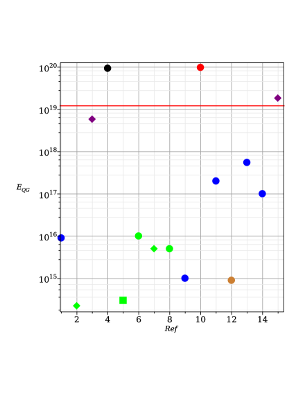
Figure 1: Current upper limits of $E_{QG}$: P1 Ellis et al. (2006), P2 Du et al. (2021), P3 Acciari et al. (2020), P4 Vasileiou et al. (2013), P5 Pan et al. (2020), P6 Agrawal et al. (2021), P7 Wei et al. (2017), P8 Desai et al. (2023), P9 Xiao et al. (2022), P10 Chang et al. (2012), P11 Shao et al. (2010), P12 Vardanyan et al. (2022), P13 Staicova (2023), P14 Staicova (2023), P15 Cao et al. (2023). The red line signifies the Planck energy. The legend can be found in the text.

While the eventual LIV effect would be very small, if it is different from zero, it can also contribute to cosmology studies, providing new datasets independent of the luminosity measurements. Such datasets critically depend on the goodness of the GRB model (affecting the intrinsic time delay) and on the understanding of the propagational systematics of the messenger (affecting the other components of the time delay). Yet, they could help us look at cosmological tensions from another angle. The question of the use of GRBs in cosmology has been studied extensively, for example, using them as standardized candles Dainotti et al. (2022); Cao et al. (2022); Dainotti et al. (2023); Xu et al. (2021) (and reference therein), through the cosmographic approach Bargiacchi et al. (2023) and trying to reduce the Hubble tension Dainotti et al. (2023), in combination with BAO, supernovae and quasars and a combined cosmological parameter Staicova (2022).

In a previous paper Staicova (2023), we started our investigation on how cosmology affects such constraints. LIV can be constrained either from the different energy bands of a single event or from averaging over multiple events, or both. However, cosmology needs to be taken into account in the estimations. It is particularly important when averaging over multiple GRBs due to the different redshifts employed. In Staicova (2023), we obtained that the effect of adding cosmology may be significant for certain models and datasets. The biggest unknown in such a study is the intrinsic time delay—i.e., the possibility that the high and low-energy photons were not emitted at the same time. Since we do not have a good enough model of the GRB progenitor to predict the intrinsic time delay, we need to approximate it with a toy model. In Staicova (2023), we used the standard approximation that assumes a constant (over the energy or the luminosity) intrinsic time delay, common for all the GRBs.

Here, we change that approximation, with  two of the most popular other approximations. The first one is the energy-dependent intrinsic time delay introduced in Wei et al. (2017); Ganguly and Desai (2017), which yields as bound for the quantum gravity energy scale $E_{QG,1}\geq 0.3\times 10^{15}$ GeV from GRB 160625B and 23 more GRBs Pan et al. (2020) and $E_{QG}^{1}\geq 10^{16}$ GeV Agrawal et al. (2021). The other is the luminosity-dependent approximation for which the previously published result is $E_{QG}^{1}\geq 10^{15}$ GeV Vardanyan et al. (2022).

In this paper, we use these two extended approximations for the intrinsic time delay and we apply them to two available GRB time delay (TD) datasets, to which we add several robust cosmological datasets. These are the angular baryonic acoustic oscillations (transversal BAO), supernovae type IA (the Pantheon Plus dataset), and the CMB distance prior. To the standard $\Lambda$CDM model, we add two dark energy (DE) models and a spatial curvature model ($\Omega_{K}$CDM). We show that at the current level of precision for the LIV parameters, the cosmology is more affected by the priors on the $c/H_{0}r_{d}$ parameter than by the intrinsic time delay approximation. We see that indeed the extended approximation has an effect on our measurement of the LIV parameter $\alpha$, but in most cases it is small. The other LIV parameters remain largely unconstrained.

The paper is organized as follows: in Section 2, we discuss the Theoretical background. In Section 3, we describe our Methods. In Section 4, we elaborate on our Datasets. In Section 5, we discuss the numerical results, and in Section 6, one can find a Discussion of the obtained results.

2 Theoretical Setup

2.1 Definition of the LIV Time Delay

We consider a modified dispersion relation for photons Amelino-Camelia et al. (1998); Vasileiou et al. (2013) of the type:

$$E^{2}=p^{2}c^{2}\left[1-s_{\pm}\left(\frac{E}{E_{QG,n}}\right)^{n}\,\right]\,,$$ (1)

with $E_{QG}$—the energy of the QG scale, $c$ is the speed of light, $p$ and $E$—the momentum and energy of photons and the $s_{\pm}=\pm 1$ for subluminal or superluminal propagation Vasileiou et al. (2013). Here, we work only with $n=1$ and subluminal LIV.

Following Jacob and Piran (2008); Biesiada and Piorkowska (2007, 2009), the time delay between a low-energy ($E_{low}$) and a high-energy ($E_{high}$) photon with $\Delta E=E_{high}-E_{low}$ in the subluminal case is

$$\Delta t_{LIV}=\frac{\Delta E}{E_{QG}}\int_{0}^{z}(1+z^{\prime})\frac{dz^{\prime}}{H(z^{\prime})}$$ (2)

where $H(z)=H_{0}E(z)$ is the Hubble parameter, $H_{0}$—the Hubble constant at $z=0$ and $E(z)$—the equation of state of the Universe.

2.2 Different LIV Approximations

The observed time delay is a combination of the quantum-gravity time delay, the intrinsic time delay and different propagational effects Zou et al. (2018); Alves Batista and Saveliev (2021); Saveliev and Alves Batista (2023). While the propagational effects can be ignored for high-energy photons, to put bounds on the quantum gravity time delay, we need to make an approximation for the intrinsic time delay. Here, we will compare the standard approximation with two of the most popular other approximations.

1.Standard approximation (e.g., Ellis et al. (2006); Biesiada and Piorkowska (2009); Pan et al. (2015); Zou et al. (2018)). For it, one assumes the following forms for the intrinsic time delay: $\Delta t_{\rm int}=\beta\left(1+z\right)$, where $\beta$ is a free parameter.

In this case, for the GRB time delay, one obtains:

$$\frac{\Delta t_{obs}}{1+z}=a_{LIV}K+\beta\,,$$ (3)

where $a_{LIV}\equiv\Delta E/(H_{0}E_{QG})$, and

$$K\equiv\frac{1}{1+z}\int_{0}^{z}\frac{(1+\tilde{z})\,d\tilde{z}}{E(\tilde{z})}\,.$$ (4)

If $a_{LIV}=0$, there is no LIV, while if $a_{LIV}\not=0$, there is LIV on energy scales above $E_{QG}$. The connection between the QG effect and cosmology comes from the term $E(z)$.

In our models, we use the form

$$\Delta t_{obs}=a_{LIV}(1+z)K+\beta\left(1+z\right)\,.$$ (5)

As in our previous paper Staicova (2023), we denote $a_{LIV}=\alpha$ and $b$ is replaced with $\beta$, to avoid mixing this parameter with $b=c/(H_{0}r_{d})$.

2. The energy-dependent approximation This approximation has been used in Wei et al. (2017); Pan et al. (2020); Agrawal et al. (2021); Desai et al. (2023) and also in Du et al. (2021) with ($\alpha\to-\alpha$). This popular formula assumes that in the source frame, the intrinsic positive time lag increases with the energy $E$ as a power law:

$$\delta t_{int}=\tau\left[\left(\frac{E}{keV}\right)^{\alpha}-\left(\frac{E_{0}}{keV}\right)^{\alpha}\right]$$ (6)

Here, $E_{0}=11.34$ keV is the median value of the fixed lowest energy band (10–12 keV). The free parameters are $\tau$ and $\alpha$. While this fit is usually associated with studying a single GRB in multiple energy bands, Desai et al. (2023) has also applied it to multiple GRBs. Note, from here on, we rename the parameters as follows: $\alpha\to\gamma,\tau\to\beta$. This is in order to differentiate them from the LIV $\alpha$ and the cosmological $b$.

3. Intrinsic GRB lag-luminosity relation approximation

This formula has been used in Vardanyan et al. (2022) to describe the intrinsic time delay of long GRBs.

$$\tau_{RF}^{int}=\tau_{obs}^{int}/(1+z)=\beta_{long}\left(\frac{L_{iso}}{L_{*}}\right)^{\gamma}$$ (7)

Here, $L_{*}$ is arbitrary normalization, and $\gamma$ and $\beta_{long}$ are the free parameters. For short GRBs, one takes $\gamma=0$, which recovers the standard approximation.

2.3 Cosmology

The equation of state of the Universe for a flat Friedmann-Lemaître-Robertson-Walker metric with the scale parameter $a=1/(1+z)$ is:

$$E(z)^{2}=\Omega_{m}(1+z)^{3}+\Omega_{DE}(z)+\Omega_{K}(1+z)^{2},$$ (8)

where $\Omega_{DE}(z)\to\Omega_{\Lambda}$ for $\Lambda$CDM. The  expansion of the universe is governed by $E(z)=H(z)/H_{0}$, where $H(z):=\dot{a}/a$ is the Hubble parameter at redshift $z$. $\Omega_{m}$, $\Omega_{K}$ and $\Omega_{DE}$ are the fractional matter, spatial and dark energy densities at redshift $z=0$.

We will consider a few dynamical dark energy models: number of different DE models: Chevallier-Polarski-Linder (CPL, Chevallier and Polarski (2001); Linder and Huterer (2005); Barger et al. (2006)) and Barboza-Alcaniz (BA Barboza and Alcaniz (2008); Escamilla-Rivera and Nájera (2022)). The relevant equations for $\Omega_{DE}(z)$ for Equation (8) can be found in Table 1. For $w_{0}=-1,w_{a}=0$ one recovers $\Lambda$CDM.

Table 1: The DE models we use in this work. The references can be found in the text.

Model	$\Omega_{DE}(z)$	$w(z)$
CPL	$\Omega_{\Lambda}\times\exp\left[\int_{0}^{z}\frac{3(1+w(z^{\prime}))dz^{\prime}}{1+z^{\prime}}\right]$	$w_{0}+w_{a}\frac{z}{z+1}$
BA	$\Omega_{\Lambda}\times(1+z)^{3(1+w_{0})}{(1+z^{2})}^{\frac{3w_{1}}{2}}$	$w_{0}+z\frac{1+z}{1+z^{2}}w_{1}$

To infer the cosmological parameters, we need to define the angular diameter distance $D_{\textrm{A}}$:

$$D_{\textrm{A}}=\frac{c}{(1+z)H_{0}\sqrt{|\Omega_{K}|}}\textrm{sinn}\left[|\Omega_{K}|^{1/2}\int_{0}^{z}\frac{dz^{\prime}}{E(z^{\prime})}\right]\ ,$$ (9)

where $\textrm{sinn}(x)\equiv\textrm{sin}(x)$, $x$, $\textrm{sinh}(x)$ for $\Omega_{K}<0$, $\Omega_{K}=0$, $\Omega_{K}>0$, respectively.

It connects to the transversal BAO measurements through the angular scale measurement $\theta_{BAO}(z)$:

$$\theta_{BAO}\left(z\right)=\frac{r_{d}}{\left(1+z\right)D_{A}(z)}.$$ (10)

The Pantheon Plus datasets measure the distance modulus $\mu(z)$, which is related to the luminosity distance ($d_{L}=D_{A}(1+z)^{2}$) in Mpc through

$$\mu_{B}(z)-M_{B}=5\log_{10}\left[d_{L}(z)\right]+25\,,$$ (11)

where $M_{B}$ is the absolute magnitude.

Finally, we include the CMB through the distance priors datapoints provided by Chen et al. (2019):

$$l_{\textrm{A}}=(1+z_{*})\frac{\pi D_{\textrm{A}}(z_{*})}{r_{s}(z_{*})},$$

$$R\equiv(1+z_{*})\frac{D_{\textrm{A}}(z_{*})\sqrt{\Omega_{m}}H_{0}}{c},$$

where $l_{\textrm{A}}$ is the acoustic scale coming from the CMB temperature power spectrum in the transverse direction and $R$ is the “shift parameter” obtained from the CMB temperature spectrum along the line-of-sight direction Komatsu et al. (2009). $r_{s}(z_{*})$ is the co-moving sound horizon at redshift photon decoupling $z_{*}$ ( $z_{*}\approx 1089$ Aghanim et al. (2020)).

3 Methods

The idea of the method is to avoid setting priors on $H_{0}$ and $r_{d}$ by considering only the quantity $b=c/(H_{0}r_{d})$. The method has been outlined in Staicova (2023). For this reason, we just list the different likelihoods here. For BAO we have

$$\chi^{2}_{BAO}=\sum_{i}\frac{\left(\vec{v}_{obs}-\vec{v}_{model}\right)^{2}}{\sigma^{2}}.$$ (12)

Here, $\vec{v}_{obs}$ is a vector of the observed points, for BAO corresponding to $\theta_{BAO,obs}^{i}$, $\vec{v}_{model}$ is the theoretical prediction of the model (for BAO —$\theta_{BAO,theor}(z_{i})$) and $\sigma$ is the error of each measurement.

For the SN dataset, we marginalize over $H_{0}$ and $M_{B}$. The integrated $\chi^{2}$ in this case is (Di Pietro and Claeskens (2003); Nesseris and Perivolaropoulos (2004); Perivolaropoulos (2005); Lazkoz et al. (2005)):

$$\tilde{\chi}^{2}_{SN,GRB}=D-\frac{E^{2}}{F}+\ln\frac{F}{2\pi},$$ (13)

for

$$D=\sum_{i}\left(\Delta\mu\,C^{-1}_{cov}\,\Delta\mu^{T}\right)^{2},$$ (14)

$$E=\sum_{i}\left(\Delta\mu\,C^{-1}_{cov}\,\boldsymbol{\mathit{E}}\right),$$

$$F=\sum_{i}C^{-1}_{cov},$$

where $\mu^{i}$ is the observational distance modulus, $\sigma_{i}$ is its error, and the $d_{L}(z)$ is the luminosity distance, $\Delta\mu=\mu^{i}-5\log_{10}\left[d_{L}(z_{i})\right)$, $\boldsymbol{\mathit{E}}$ is the unit matrix, and $C^{-1}_{cov}$ is the inverse covariance matrix of the Pantheon Plus dataset as given by Scolnic et al. (2022); Brout et al. (2022).

Finally, we define the time delay likelihood as Equation (12), but here, the quantity we consider is the theoretical time delay ($\vec{\Delta t}_{model}$), as defined in Equation (5) and its observational value (($\vec{\Delta t}_{obs}$), which is provided by the TD dataset.

$$\chi^{2}_{TD}=\sum_{i}\frac{\left(\vec{\Delta t}_{obs}-\vec{\Delta t}_{model}\right)^{2}}{\sigma^{2}},$$ (15)

The final $\chi^{2}$ is

$$\chi^{2}=\chi^{2}_{BAO}+\chi^{2}_{CMB}+\chi^{2}_{SN}+\chi^{2}_{TD}$$

4 Datasets

In this work, we use the so-called transversal BAO dataset published by Nunes et al. (2020), for which the authors claim to be cleaned up from the dependence on the cosmological model and uncorrelated. The CMB distant prior is given by Chen et al. (2019). The SN data comes from the Pantheon Plus dataset. It consists of 1701 light curves of 1550 spectroscopically confirmed Type Ia supernovae and their covariances, from which distance modulus measurements have been obtained Riess et al. (2022); Brout et al. (2022); Scolnic et al. (2022).

To study the time delays, we use two different time delays (TD) datasets—TD1 provided by Vardanyan et al. (2022) and TD2 Xiao et al. (2022). TD1 uses a combined sample of 49 long and short GRBs observed by Swift, dating between 2005 to 2013. In this dataset Bernardini et al. (2015); Vardanyan et al. (2022), the time lags have been extracted through a discrete cross-correlation function (CCF) analysis between characteristic rest-frame energy bands of 100–150 keV and 200–250 keV. The redshift for TD1 is $z\in[0.35,5.47]$. TD2 Xiao et al. (2022) uses 46 short GRBs with measured redshifts at Fixed Energy Bands (15–70 keV and 120–250 keV) gathered between 2004 and 2020 by Swift/BAT or Fermi/GBM. The two datasets have only six common GRBs, which is under 15% of their total number (49 vs. 46 events), which makes them effectively uncorrelated and independent. Because we want to emphasize the effect of cosmology, we prefer to average over multiple GRBs rather than to use measurements from a single GRB  Ellis et al. (2006).

To run the inference, we use a nested sampler, provided by the open-source package $Polychord$ Handley et al. (2015) and the package $GetDist$ package Lewis (2019) for the plots.

We use uniform priors for all quantities: $\Omega_{m}\in[0.1,1.]$, $\Omega_{\Lambda}\in[0.,1-\Omega_{m}]$, $c/(H_{0}r_{d})\in[25,35]$, $w_{0}\in[-1.5,-0.5]$ and $w_{a}\in[-0.5,0.5]$. Since the distance prior is defined at the decoupling epoch ($z_{*}$) and the BAO—at drag epoch ($z_{d}$), we parametrize the difference between $r_{s}(z_{*})$ and $r_{s}(z_{d})$ as $rat=r_{*}/r_{d}$, where the prior for the ratio is $rat\in[0.9,1.1]$ . The LIV priors are $\alpha\in[0,0.1],\beta\in[-1,1],\gamma\in[-3,0]$.

5 Results

In Staicova (2023), we started investigating the effect of cosmology on LIV bounds by studying in the standard approximation (Equation (3)) two databases: the most famous and robust time delay dataset published by Ellis et al. Ellis et al. (2006) and the one that we currently refer to as TD1. To avoid repetition. In this section, we present only the extended approximationsWhen we refer to the “extended model”, we will mean the Intrinsic GRB lag-luminosity relation (Equation (6)) approximation for TD1 and the Energy-dependent approximation (Equation (7)) for TD2.. For completeness, the results for the standard approximation for TD1 and TD2 are presented in Appendix C.

Since our previous work Staicova (2023) demonstrated a deviation from the expected values for $b$ and $\Omega_{m}$, here, we want to investigate further this observation. To this end, we try two hypotheses for the two datasets—a uniform prior on $b$ and a Gaussian prior focused on the expected value from Planck results, $b=30\pm 1$. For the standard approximation, this leads to a very clear higher value of $\Omega_{m}$ but a minimal difference for the DE parameters $w_{0}$ and $w_{a}$ and $\Omega_{K}$.

The results for the extended models are summarized below.

• Matter density

In Figure 2, one can see the plot of $b$ vs. $\Omega_{m}$ for the extended LIV models for the four different cosmological models we consider (and the two priors on $b$).

Figure 2: Posteriors (95%CL and 68% CL) for the TD1 dataset (left) and the TD2 dataset (right) for the parameters $b$ and $\Omega_{m}$.

For both datasets, we see two groups of posteriors—one grouped around the top right corner, which corresponds to the Gaussian priors on $b$, and one that spans across the whole interval for the uniform prior. In both cases, the mean value and the 95% CL of $b$ are below the expected value of $b\sim 30$ for the three models.

For TD1, setting the Gaussian prior for $b$ in this case significantly constrains $\Omega_{m}$ and puts it in the limits of [0.29,0.34] at 95% CL. In this case, $\Omega_{k}$CDM gives the highest mean $\Omega_{m}$ and $CPL$ gives the lowest one, with $\Lambda$CDM in between. For the uniform prior, the posterior for $\Omega_{m}$ is much less constrained, with the lowest value coming from $\Omega_{K}$CDM and the posteriors for $\Lambda$CDM and CPL largely coinciding.

For the other dataset, TD2, the situation repeats to a great extent, with a little bit higher matter density $\Omega_{m}\in[0.3,0.34]$ for the Gaussian prior and $b\in[27.8,29,2]$ and the lowest value for $\Omega_{m}$ is for $\Lambda$CDM and the highest for $\Omega_{K}$CDM. For the uniform prior, we have again the lowest value for $\Omega_{m}$ and $b$ coming from $\Omega_{K}$CDM and $\Lambda$CDM and CPL largely coinciding.

• Spatial curvature

The results for $\Omega_{K}$CDM are presented in Figure 3.

Figure 3: Posteriors (95%CL and 68% CL) for the TD1 dataset (left) and the TD2 dataset (right)—the spatial curvature $\Omega_{K}$ vs. $\Omega_{m}$.

We see that our results are not consistent with a flat universe at the 95% CL even for a uniform prior on $b$. For TD1, we get a bit less constrained contours for $\Omega_{K}$, but more constrained than the flat cases. A rather interesting feature is the huge difference in $\Omega_{m}$ between the uniform and the Gaussian cases for both datasets. Our prior on $\Omega_{K}$ is relatively small ($\Omega_{K}\in[-0.1,0.1]$), however, due to the large number of parameters of the model.

• DE parameters

The two DE models we consider are shown in Figure 4. Their DE parameters $w_{0}$ and $w_{a}$ are largely insensitive to the dataset and their mean values for $w_{0}$ are lower than expected for $\Lambda$CDM, with $w_{0}\sim-0.8$. This is a different value from the one obtained Staicova (2023), which was consistent with $\Lambda$CDM at 68% CL. The result in the study Staicova (2022) without TD on the other hand, shows values about $w_{0}\sim-1.1$. In the two latter works, we use the Pantheon dataset, while here, we use the Pantheon Plus. To clarify if the difference is due to the new SN dataset or to the new TD datasets, we ran the same experiment with Pantheon instead of Pantheon Plus and it gave $w_{0}\to-1$ within 68% CL. As expected, the parameter $w_{0}$ is well constrained by the data while $w_{a}$ is not constrained at all.

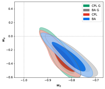
Figure 4: Posteriors (95%CL and 68% CL) for the TD1 dataset (left) and the TD2 dataset (right) in the $w_{0}-w_{a}$ plane.

Note, the cosmological results for TD1 and TD2 for the extended models look largely the same. That could be due to similar treatment of the data or other reasons (like adding additional degrees of freedom in the extended models). The standard approximation posteriors presented in Appendix A show a larger dependence on the dataset. Also, the LIV contribution to the fit is quite small due to the smallness of $\alpha$. As long as it is non-negligible, it still contributes to the cosmology in a minor way, as seen above in $b$ and $\Omega_{m}$. The numerical experiment shows that for the TD1 dataset, the effect of the TD dataset on the cosmology becomes really pronounced at about $\alpha\sim 10^{-2}$, while for TD2, it becomes pronounced at about $\alpha\sim 10^{-3}$. This is just an order or two above our current constraints for $\alpha$. This means that observing an event that would push the bound for $E_{QG}$ lower (or having a GRB intrinsic time delay model that would do so) would also bring the TD measurement on par with the current cosmological probes.

• LIV Parameters

Finally, we are going to discuss the LIV parameters, $\alpha,\beta$ and $\gamma$. They are shown in Figures 5 and 6. In Figure 5, we can see the values for $\alpha$ we obtained (where it should be noted that the lower bound on $\alpha$ is, of course, $0$). As a whole, TD1 gives 10 times higher values for $\alpha$ than $TD2$ (which has been noticed also in our previous paper). We also see that the extended models do not have a conclusive improvement over the standard approximation, even though, for some of the models considered, they lead to significantly smaller $\alpha$, meaning higher $E_{QG}$.

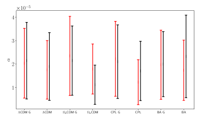
Figure 5: Mean values and errors for the parameter $\alpha$ for the standard approximation (red) and the extended one (black) different models. To the (left) are the results for TD1 and to the (right)—from TD2.

In Figure 6, we show the parameters $\beta$ and $\gamma$. We note that they are mostly unconstrained in all of the models and while there are differences between the standard and the extended approximations, they are minor. The posteriors for the LIV parameters can be found in Appendix B.

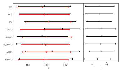
Figure 6: Mean values and errors (68%CL) for the parameters $\beta$ and $\gamma$ for the standard approximation (red) and the extended one (black) different models. To the (left) are the results for TD1 and to the (right)—from TD2.

To obtain the values for $E_{QG}$, one needs to use the formula $E_{QG}=\Delta E/(H_{0}a_{LIV})$. This requires inputting the specific energy band for each dataset ($\Delta E$), and choosing a value for $H_{0}$. The error in this case will be

$$\sigma(E_{EQ})=E_{QG}\sqrt{\frac{{\sigma_{H0}}^{2}}{{H_{0}}^{2}}+\frac{{\sigma_{\alpha}}^{2}}{\alpha^{2}}}.$$

Since $\alpha=0$ is the low limit of our priors, which gives an upper bound for $E_{QG}$ infinity, we can get only the lower bound of the quantum gravity energy. We take as $\sigma_{\alpha}$ the 68% CL corresponding to $1\sigma$ deviation and we take the minimal and the maximal energies obtained for the different models. The results can be found in Table 2. In it, one needs to remember that the error comes from the incertitude in $H_{0}$ and the numerical estimation of $\alpha$; thus, it is not supposed to be taken as a measurement, but as an estimation of the error we get from this study.

Table 2: The minimal and maximal energy $E_{QG}$ for the standard approximation (SA) and the extended approximation (EA).

Dataset	$E_{QG}^{min,SA}\times 10^{17}$Gev	$E_{QG}^{max,SA}\times 10^{17}$Gev	$E_{QG}^{min,EA}\times 10^{17}$Gev	$E_{QG}^{max,EA}\times 10^{17}$Gev
$H_{0}=73.04\pm 1.04$
TD1	$1.14\pm 0.84$	$0.81\pm 0.57$	$1.39\pm 1.01$	$0.93\pm 0.68$
TD2	$48.0\pm 35.6$	$35.5\pm 25.5$	$74.6\pm 55.9$	$35.8\pm 27.1$
$H_{0}=67.4\pm 0.5$
TD1	$1.24\pm 0.91$	$0.88\pm 0.62$	$1.51\pm 1.09$	$1.01\pm 0.735$
TD2	$48.0\pm 35.6$	$35.5\pm 25.5$	$74.6\pm 55.9$	$35.8\pm 27.1$

6 Discussion

We have studied the LIV bounds and the effect of cosmology based on two different datasets TD1 Bernardini et al. (2015); Vardanyan et al. (2022) and TD2 Xiao et al. (2022). To allow testing for new approximations for the intrinsic time delay, we have added two extended models—the intrinsic GRB lag-luminosity relation approximation for TD1 and the energy-dependent approximation for TD2 and we have compared them to the standard approximation (“constant” intrinsic time, i.e., not depending on the energy or the luminosity). To study the effect of the cosmological model, we have used additional cosmological datasets including transversal BAO, the Pantheon Plus dataset and the CMB distance priors. These are some of the most robust cosmological datasets; thus, they provide the best opportunity to study the joint effect of cosmology and LIV. We have considered $\Lambda$CDN, $\Omega_{K}$CDM, the CPL and the BA dark energy models.

From the results we obtain, we see that the strongest effect is due to the prior on the parameter $\frac{c}{H_{0}r_{d}}$ and not so much on the approximation for the intrinsic lag. This is because first the LIV effect is expected to be very small, and second, the intrinsic lag parameters are largely unbound from the current data. Instead, we see that the results for $\alpha$ depend a lot on the cosmological model. The lowest bounds of $E_{QG}$ are for $\Omega_{K}$CDM and the highest for $\Lambda$CDM G (TD1) and BA (TD2). Surprisingly, despite the new degrees of freedom introduced by the LIV parameters, the $\Omega_{K}$CDM model suggests a closed universe. In terms of LIV energy, we obtain as lowest bound for TD1 $E_{QG}>0.8\times 10^{17}$ GeV and for TD2: $E_{QG}>3.5\times 10^{18}$ GeV. In both cases, the error is significant, regardless of the small error of $H_{0}$. TD1 tends to give 10 times larger values of $\alpha$ than TD2. The effect of the TD datasets on the cosmological parameters becomes noticeable if $\alpha$ is an order higher than the inferred one, meaning lower than the currently estimated $E_{QG}$.

In conclusion, we see that for the moment, the time delay datasets are not precise enough to constrain the cosmological effects, while the cosmological models have a serious effect on the LIV constraints. For this situation to change, we need to improve the model of the GRB central engine and also to be able to better constrain the propagational effects, which are considered negligible at high energies; however, one needs to remember that not all measurements are made at very high energies, especially for the older GRB collections. Finally, a new and better approximation for the intrinsic time delay could benefit both GRB theoretical models and cosmological studies.

This work was conducted in a Short Term Scientific Missions (STSM) in Spain, funded by the COST Action CA21136 “Addressing observational tensions in cosmology with systematics and fundamental physics (CosmoVerse)”.

Appendix A Posteriors of the Models

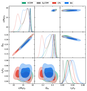
Figure 7: Posteriors for the TD1 dataset for the standard approximation (left panel) and the extended approximation (right panel). On each panel, the uniform prior is on the bottom triangle plot, the Gaussian—on the top one.

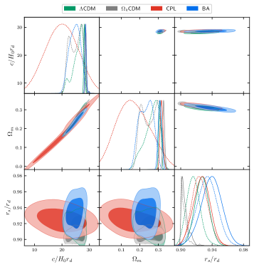
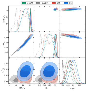
Figure 8: Posteriors for the TD2 dataset for the standard approximation (left panel) and the extended approximation (right panel). On each panel, the uniform prior is on the bottom triangle plot, the Gaussian—on the top one.

Appendix B LIV Parameters Posteriors

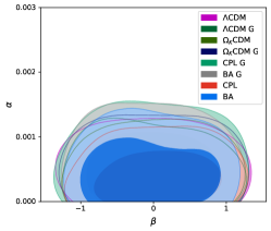
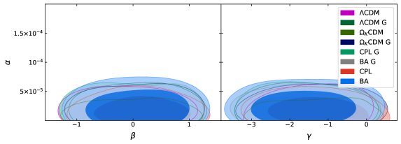
Figure 9: Posteriors (95% CL and 68% CL) for the TD1 dataset (top panel) and the TD2 dataset (bottom panel). On the left, we have the SA case with its two parameters $\alpha$ and $\beta$, on the right, the EA case with its three parameters $\alpha$, $\beta$ and $\gamma$. As seen for the plots, only $\alpha$ can be bounded with these datasets.

Appendix C Tables of the Results

Table 3: Mean values for the TD1 dataset for the standard approximation.

Model	$c/H_{0}r_{d}$	$\Omega_{K}$	$\Omega_{m}$	$r_{s}/r_{d}$	$w_{0}$	$w_{a}$
$\Lambda$CDM G	$28.7\pm 0.3$	0.000	$0.33\pm 0.01$	$0.92\pm 0.01$	0.000	0.000
$\Lambda$CDM	$26.7\pm 1.9$	0.000	$0.28\pm 0.04$	$0.92\pm 0.01$	0.000	0.000
$\Omega_{K}$CDM G	$28.6\pm 0.2$	$-9.95\pm 1.81$	$0.33\pm 0.01$	$0.91\pm 0.0$	0.000	0.000
$\Omega_{K}$CDM	$26.6\pm 1.4$	$-7.30\pm 1.85$	$0.29\pm 0.03$	$0.9\pm 0.0$	0.000	0.000
CPL G	$28.7\pm 0.2$	0.000	$0.32\pm 0.01$	$0.93\pm 0.01$	$-0.84\pm 0.03$	$-0.3\pm 0.15$
CPL	$25.1\pm 3.2$	0.000	$0.25\pm 0.06$	$0.92\pm 0.01$	$-0.84\pm 0.03$	$-0.33\pm 0.13$
BA G	$28.6\pm 0.2$	0.000	$0.31\pm 0.01$	$0.94\pm 0.01$	$-0.8\pm 0.05$	$-0.31\pm 0.14$
BA	$26.1\pm 1.7$	0.000	$0.26\pm 0.04$	$0.93\pm 0.01$	$-0.8\pm 0.04$	$-0.34\pm 0.13$

Table 4: Mean values for the TD1 dataset for the extended approximation.

Model	$c/H_{0}r_{d}$	$\Omega_{K}$	$\Omega_{m}$	$r_{s}/r_{d}$	$w_{0}$	$w_{a}$
$\Lambda$CDM GL	$28.2\pm 0.2$	0.000	$0.31\pm 0.01$	$0.93\pm 0.01$	0.000	0.000
$\Lambda$CDM L	$25.5\pm 2.5$	0.000	$0.26\pm 0.05$	$0.92\pm 0.01$	0.000	0.000
$\Omega_{K}$CDM GL	$28.5\pm 0.2$	$-9.44\pm 1.97$	$0.33\pm 0.01$	$0.91\pm 0.0$	0.000	0.000
$\Omega_{K}$CDM L	$19.0\pm 1.1$	$-3.84\pm 9.06$	$0.15\pm 0.02$	$0.9\pm 0.0$	0.000	0.000
CPL GL	$28.3\pm 0.3$	0.000	$0.31\pm 0.01$	$0.92\pm 0.01$	$-0.84\pm 0.03$	$-0.32\pm 0.14$
CPL L	$26.0\pm 2.1$	0.000	$0.27\pm 0.04$	$0.92\pm 0.01$	$-0.84\pm 0.03$	$-0.32\pm 0.13$
BA GL	$28.8\pm 0.2$	0.000	$0.31\pm 0.01$	$0.94\pm 0.01$	$-0.79\pm 0.04$	$-0.33\pm 0.12$
BAL	$26.9\pm 1.2$	0.000	$0.28\pm 0.02$	$0.93\pm 0.01$	$-0.81\pm 0.05$	$-0.3\pm 0.14$

Table 5: Mean values for the TD2 dataset for the standard .

Model	$c/H_{0}r_{d}$	$\Omega_{K}$	$\Omega_{m}$	$r_{s}/r_{d}$	$w_{0}$	$w_{a}$
$\Lambda$CDM G	$28.1\pm 0.2$	0.000	$0.31\pm 0.01$	$0.93\pm 0.01$	0.000	0.000
$\Lambda$CDM	$25.7\pm 1.9$	0.000	$0.27\pm 0.04$	$0.92\pm 0.01$	0.000	0.000
$\Omega_{K}$CDM G	$28.5\pm 0.2$	$-9.85\pm 1.82$	$0.33\pm 0.01$	$0.91\pm 0.0$	0.000	0.000
$\Omega_{K}$CDM	$25.0\pm 2.7$	$-6.73\pm 2.27$	$0.25\pm 0.05$	$0.9\pm 0.0$	0.000	0.000
CPL G	$28.6\pm 0.3$	0.000	$0.32\pm 0.01$	$0.93\pm 0.01$	$-0.83\pm 0.03$	$-0.34\pm 0.13$
CPL	$19.9\pm 6.9$	0.000	$0.17\pm 0.1$	$0.92\pm 0.01$	$-0.84\pm 0.03$	$-0.35\pm 0.11$
BA G	$28.6\pm 0.2$	0.000	$0.31\pm 0.01$	$0.94\pm 0.01$	$-0.8\pm 0.05$	$-0.31\pm 0.13$
BA	$24.7\pm 2.3$	0.000	$0.23\pm 0.04$	$0.93\pm 0.01$	$-0.81\pm 0.05$	$-0.31\pm 0.14$

Table 6: Mean values for the TD2 dataset for the extended approximation.

Model	$c/H_{0}r_{d}$	$\Omega_{K}$	$\Omega_{m}$	$r_{s}/r_{d}$	$w_{0}$	$w_{a}$
$\Lambda$CDM GL	$28.2\pm 0.2$	0.000	$0.31\pm 0.01$	$0.93\pm 0.01$	0.000	0.000
$\Lambda$CDM L	$25.1\pm 2.1$	0.000	$0.25\pm 0.05$	$0.92\pm 0.01$	0.000	0.000
$\Omega_{K}$CDM GL	$28.4\pm 0.2$	$-9.26\pm 1.63$	$0.33\pm 0.01$	$0.9\pm 0.0$	0.000	0.000
$\Omega_{K}$CDM L	$19.5\pm 1.2$	$-4.04\pm 1.09$	$0.15\pm 0.02$	$0.91\pm 0.0$	0.000	0.000
CPL GL	$28.7\pm 0.3$	0.000	$0.32\pm 0.01$	$0.93\pm 0.01$	$-0.82\pm 0.03$	$-0.33\pm 0.13$
CPL L	$24.9\pm 2.5$	0.000	$0.25\pm 0.05$	$0.92\pm 0.01$	$-0.83\pm 0.03$	$-0.34\pm 0.12$
BA GL	$28.6\pm 0.2$	0.000	$0.31\pm 0.01$	$0.94\pm 0.01$	$-0.79\pm 0.04$	$-0.34\pm 0.11$
BAL	$25.4\pm 2.1$	0.000	$0.25\pm 0.04$	$0.93\pm 0.01$	$-0.8\pm 0.05$	$-0.32\pm 0.13$

Table 7: The LIV parameters for TD1: to the left—the standard approximation, to the right—the extended one.

Model	B	$\beta$	$\alpha\times 10^{-4}$	$\beta$	$\gamma$
$\Lambda$CDM G	$4.01\pm 2.82$	$-0.06\pm 0.65$	$4.56\pm 3.34$	$0.006\pm 0.7$	$-1.65\pm 0.93$
$\Lambda$CDM	$4.46\pm 3.08$	$0.02\pm 0.63$	$4.34\pm 2.87$	$0.18\pm 0.71$	$-1.38\pm 0.86$
$\Omega_{K}$CDM G	$4.73\pm 3.36$	$-0.008\pm 0.64$	$4.27\pm 3.18$	$-0.08\pm 0.69$	$-1.45\pm 1.11$
$\Omega_{K}$CDM	$4.11\pm 3.02$	$0.03\pm 0.64$	$3.04\pm 2.21$	$-0.09\pm 0.67$	$-1.35\pm 1.1$
CPL G	$5.21\pm 3.66$	$-0.02\pm 0.65$	$3.85\pm 2.72$	$0.43\pm 0.47$	$-1.46\pm 1.11$
CPL	$3.69\pm 2.69$	$0.07\pm 0.6$	$4.26\pm 3.06$	$0.11\pm 0.68$	$-1.55\pm 0.93$
BA G	$5.06\pm 3.95$	$-0.03\pm 0.66$	$3.99\pm 3.10$	$-0.02\pm 0.68$	$-1.52\pm 0.99$
BA	$4.57\pm 3.32$	$-0.09\pm 0.67$	$3.86\pm 3.00$	$-0.03\pm 0.69$	$-1.48\pm 1.06$

Table 8: The LIV parameters for TD2: to the left—the standard approximation, to the right—the extended one.

Model	$\alpha\times 10^{-5}$	$\beta$	$\alpha\times 10^{-5}$	$\beta$	$\gamma$
$\Lambda$CDM G	$2.03\pm 1.49$	$0.01\pm 0.66$	$2.15\pm 1.64$	$0.14\pm 0.66$	$-1.59\pm 1.0$
$\Lambda$CDM	$1.75\pm 1.25$	$-0.23\pm 0.6$	$1.90\pm 1.45$	$-0.14\pm 0.62$	$-1.57\pm 0.81$
$\Omega_{K}$CDM G	$2.35\pm 1.69$	$-0.14\pm 0.62$	$2.15\pm 1.48$	$0.06\pm 0.7$	$-1.41\pm 0.89$
$\Omega_{K}$CDM	$1.79\pm 1.07$	$-0.15\pm 0.54$	$1.12\pm 0.84$	$-0.06\pm 0.66$	$-1.27\pm 0.96$
CPL G	$2.22\pm 1.60$	$-0.15\pm 0.57$	$2.10\pm 1.57$	$-0.06\pm 0.63$	$-1.61\pm 0.96$
CPL	$1.23\pm 0.96$	$-0.29\pm 0.54$	$1.71\pm 1.27$	$0.16\pm 0.61$	$-1.27\pm 0.98$
BA G	$1.97\pm 1.47$	$0.03\pm 0.69$	$2.00\pm 1.39$	$0.06\pm 0.76$	$-1.65\pm 0.96$
BA	$1.74\pm 1.29$	$0.05\pm 0.63$	$2.33\pm 1.76$	$0.09\pm 0.69$	$-1.62\pm 0.91$

list-name=Note [custom]

References

References

- Abdalla et al. (2022) Abdalla, E.; Abellán, G.F.; Aboubrahim, A.; Agnello, A.; Akarsu, Ö.; Akrami, Y.; Alestas, G.; Aloni, D.; Amendola, L.; Anchordoqui, L.A.; et al. Cosmology intertwined: A review of the particle physics, astrophysics, and cosmology associated with the cosmological tensions and anomalies. J. High Energy Astrophys. 2022, 34, 49–211. https://doi.org/10.1016/j.jheap2022.04.002.
- Vagnozzi (2023) Vagnozzi, S. Seven Hints That Early-Time New Physics Alone Is Not Sufficient to Solve the Hubble Tension. Universe 2023, 9, 393. https://doi.org/10.3390/universe9090393.
- Benisty et al. (2023) Benisty, D.; Mifsud, J.; Levi Said, J.; Staicova, D. On the robustness of the constancy of the Supernova absolute magnitude: Non-parametric reconstruction & Bayesian approaches. Phys. Dark Univ. 2023, 39, 101160. https://doi.org/10.1016/j.dark.2022.101160.
- Dainotti et al. (2022) Dainotti, M.G.; De Simone, B.; Schiavone, T.; Montani, G.; Rinaldi, E.; Lambiase, G.; Bogdan, M.; Ugale, S. On the Evolution of the Hubble Constant with the SNe Ia Pantheon Sample and Baryon Acoustic Oscillations: A Feasibility Study for GRB-Cosmology in 2030. Galaxies 2022, 10, 24. https://doi.org/10.3390/galaxies10010024.
- Dias et al. (2023) Dias, B.L.; Avila, F.; Bernui, A. Probing cosmic homogeneity in the Local Universe. Mon. Not. Roy. Astron. Soc. 2023, 526, 3219–3229. https://doi.org/10.1093/mnras/stad2980.
- Dialektopoulos et al. (2024) Dialektopoulos, K.F.; Mukherjee, P.; Levi Said, J.; Mifsud, J. Neural network reconstruction of scalar-tensor cosmology. Phys. Dark Univ. 2024, 43, 101383. https://doi.org/10.1016/j.dark.2023.101383.
- Alonso et al. (2023) Alonso, P.M.M.; Escamilla-Rivera, C.; Sandoval-Orozco, R. Constraining dark energy cosmologies with spatial curvature using Supernovae JWST forecasting. arXiv 2023, arXiv:2309.12292.
- Benisty et al. (2023) Benisty, D.; Davis, A.C.; Evans, N.W. Constraining Dark Energy from the Local Group Dynamics. Astrophys. J. Lett. 2023, 953, L2. https://doi.org/10.3847/2041-8213/ace90b.
- Dialektopoulos et al. (2023) Dialektopoulos, K.F.; Mukherjee, P.; Levi Said, J.; Mifsud, J. Neural network reconstruction of cosmology using the Pantheon compilation. Eur. Phys. J. C 2023, 83, 956. https://doi.org/10.1140/epjc/s10052-023-12124-3.
- Briffa et al. (2023) Briffa, R.; Escamilla-Rivera, C.; Levi Said, J.; Mifsud, J. Constraints on f(T) cosmology with Pantheon+. Mon. Not. Roy. Astron. Soc. 2023, 522, 6024–6034. https://doi.org/10.1093/mnras/stad1384.
- Zhai et al. (2023) Zhai, Y.; Giarè, W.; van de Bruck, C.; Di Valentino, E.; Mena, O.; Nunes, R.C. A consistent view of interacting dark energy from multiple CMB probes. JCAP 2023, 7, 032. https://doi.org/10.1088/1475-7516/2023/07/032.
- Bernui et al. (2023) Bernui, A.; Di Valentino, E.; Giarè, W.; Kumar, S.; Nunes, R.C. Exploring the H0 tension and the evidence for dark sector interactions from 2D BAO measurements. Phys. Rev. D 2023, 107, 103531. https://doi.org/10.1103/PhysRevD.107.103531.
- Yang et al. (2023) Yang, W.; Giarè, W.; Pan, S.; Di Valentino, E.; Melchiorri, A.; Silk, J. Revealing the effects of curvature on the cosmological models. Phys. Rev. D 2023, 107, 063509. https://doi.org/10.1103/PhysRevD.107.063509.
- Gariazzo et al. (2022) Gariazzo, S.; Di Valentino, E.; Mena, O.; Nunes, R.C. Late-time interacting cosmologies and the Hubble constant tension. Phys. Rev. D 2022, 106, 023530. https://doi.org/10.1103/PhysRevD.106.023530.
- Bargiacchi et al. (2023) Bargiacchi, G.; Dainotti, M.G.; Nagataki, S.; Capozziello, S. Gamma-Ray Bursts, Quasars, Baryonic Acoustic Oscillations, and Supernovae Ia: New statistical insights and cosmological constraints. Mon. Not. R. Astron. Soc. 2023, 521, 3909–3924. https://doi.org/10.1093/mnras/stad763.
- Staicova and Stoilov (2023) Staicova, D.; Stoilov, M. Electromagnetic Waves in Cosmological Spacetime. Universe 2023, 9, 292. https://doi.org/10.3390/universe9060292.
- Dainotti et al. (2021) Dainotti, M.G.; De Simone, B.; Schiavone, T.; Montani, G.; Rinaldi, E.; Lambiase, G. On the Hubble constant tension in the SNe Ia Pantheon sample. Astrophys. J. 2021, 912, 150. https://doi.org/10.3847/1538-4357/abeb73.
- Colladay and Kostelecky (1997) Colladay, D.; Kostelecky, V.A. CPT violation and the standard model. Phys. Rev. D 1997, 55, 6760–6774. https://doi.org/10.1103/PhysRevD.55.6760.
- Amelino-Camelia et al. (1998) Amelino-Camelia, G.; Ellis, J.R.; Mavromatos, N.E.; Nanopoulos, D.V.; Sarkar, S. Tests of quantum gravity from observations of gamma-ray bursts. Nature 1998, 393, 763–765. https://doi.org/10.1038/31647.
- Colladay and Kostelecky (1998) Colladay, D.; Kostelecky, V.A. Lorentz violating extension of the standard model. Phys. Rev. D 1998, 58, 116002. https://doi.org/10.1103/PhysRevD.58.116002.
- Kostelecky and Samuel (1989) Kostelecky, V.A.; Samuel, S. Spontaneous Breaking of Lorentz Symmetry in String Theory. Phys. Rev. D 1989, 39, 683. https://doi.org/10.1103/PhysRevD.39.683.
- Ellis et al. (2006) Ellis, J.R.; Mavromatos, N.E.; Nanopoulos, D.V.; Sakharov, A.S.; Sarkisyan, E.K.G. Robust limits on Lorentz violation from gamma-ray bursts. Astropart. Phys. 2006, 25, 402–411; Erratum in Astropart. Phys. 2008, 29, 158–159. https://doi.org/10.1016/j.astropartphys.2007.12.003.
- Jacob and Piran (2008) Jacob, U.; Piran, T. Lorentz-violation-induced arrival delays of cosmological particles. JCAP 2008, 1, 031. https://doi.org/10.1088/1475-7516/2008/01/031.
- Gubitosi et al. (2009) Gubitosi, G.; Pagano, L.; Amelino-Camelia, G.; Melchiorri, A.; Cooray, A. A Constraint on Planck-scale Modifications to Electrodynamics with CMB polarization data. JCAP 2009, 8, 021. https://doi.org/10.1088/1475-7516/2009/08/021.
- Vasileiou et al. (2015) Vasileiou, V.; Granot, J.; Piran, T.; Amelino-Camelia, G. A Planck-scale limit on spacetime fuzziness and stochastic Lorentz invariance violation. Nature Phys. 2015, 11, 344–346. https://doi.org/10.1038/nphys3270.
- Amelino-Camelia et al. (2013) Amelino-Camelia, G.; Arzano, M.; Gubitosi, G.; Magueijo, J. Rainbow gravity and scale-invariant fluctuations. Phys. Rev. D 2013, 88, 041303. https://doi.org/10.1103/PhysRevD.88.041303.
- Magueijo and Smolin (2002) Magueijo, J.; Smolin, L. Lorentz invariance with an invariant energy scale. Phys. Rev. Lett. 2002, 88, 190403. https://doi.org/10.1103/PhysRevLett.88.190403.
- Amelino-Camelia and Piran (2001) Amelino-Camelia, G.; Piran, T. Planck scale deformation of Lorentz symmetry as a solution to the UHECR and the TeV gamma paradoxes. Phys. Rev. D 2001, 64, 036005. https://doi.org/10.1103/PhysRevD.64.036005.
- Amelino-Camelia (2002a) Amelino-Camelia, G. Relativity in space-times with short distance structure governed by an observer independent (Planckian) length scale. Int. J. Mod. Phys. D 2002, 11, 35–60. https://doi.org/10.1142/S0218271802001330.
- Amelino-Camelia (2002b) Amelino-Camelia, G. Doubly special relativity. Nature 2002, 418, 34–35. https://doi.org/10.1038/418034a.
- Kostelecky and Russell (2011) Kostelecky, V.A.; Russell, N. Data Tables for Lorentz and CPT Violation. Rev. Mod. Phys. 2011, 83, 11–31. https://doi.org/10.1103/RevModPhys.83.11.
- Wei and Wu (2021a) Wei, J.J.; Wu, X.F. Tests of Lorentz Invariance. In Handbook of X-ray and Gamma-ray Astrophysics; Bambi, C., Santangelo, A., Eds.; Springer: Singapore, 2021. https://doi.org/10.1007/978-981-16-4544-0_132-1.
- Wei and Wu (2021b) Wei, J.J.; Wu, X.F. Testing fundamental physics with astrophysical transients. Front. Phys. 2021, 16, 44300. https://doi.org/10.1007/s11467-021-1049-x.
- Zhou et al. (2021) Zhou, Q.Q.; Yi, S.X.; Wei, J.J.; Wu, X.F. Constraints on Lorentz Invariance Violation with Multiwavelength Polarized Astrophysical Sources. Galaxies 2021, 9, 44. https://doi.org/10.3390/galaxies9020044.
- Addazi et al. (2022) Addazi, A.; Alvarez-Muniz, J.; Batista, R.A.; Amelino-Camelia, G.; Antonelli, V.; Arzano, M.; Asorey, M.; Atteia, J.L.; Bahamonde, S.; Bajardi, F.; et al. Quantum gravity phenomenology at the dawn of the multi-messenger era—A review. Prog. Part. Nucl. Phys. 2022, 125, 103948. https://doi.org/10.1016/j.ppnp.2022.103948.
- Desai (2023) Desai, S. Astrophysical and Cosmological Searches for Lorentz Invariance Violation. arXiv 2023, arXiv:2303.10643.
- Anchordoqui et al. (2021) Anchordoqui, L.A.; Di Valentino, E.; Pan, S.; Yang, W. Dissecting the H0 and S8 tensions with Planck + BAO + supernova type Ia in multi-parameter cosmologies. J. High Energy Astrophys. 2021, 32, 28–64. https://doi.org/10.1016/j.jheap.2021.08.001.
- Abdalla et al. (2024) Abdalla, H.; Cotter, G.; Backes, M.; Kasai, E.; Böttcher, M. Investigating the Lorentz invariance violation effect using different cosmological backgrounds. Class. Quant. Grav. 2024, 41, 015022. https://doi.org/10.1088/1361-6382/ad1122.
- Pasumarti and Desai (2023) Pasumarti, V.; Desai, S. Bayesian evidence for spectral lag transition due to Lorentz invariance violation for 32 Fermi/GBM Gamma-ray bursts. J. High Energy Astrophys. 2023, 40, 41–48. https://doi.org/10.1016/j.jheap.2023.10.001.
- Bolmont et al. (2022) Bolmont, J.; Caroff, S.; Gaug, M.; Gent, A.; Jacholkowska, A.; Kerszberg, D.; Levy, C.; Lin, T.; Martinez, M.; Nogués, L.; Otte, A.N.; et al. First Combined Study on Lorentz Invariance Violation from Observations of Energy-dependent Time Delays from Multiple-type Gamma-Ray Sources. I. Motivation, Method Description, and Validation through Simulations of H.E.S.S., MAGIC, and VERITAS Data Sets. Astrophys. J. 2022, 930, 75. https://doi.org/10.3847/1538-4357/ac5048.
- Rosati et al. (2015) Rosati, G.; Amelino-Camelia, G.; Marciano, A.; Matassa, M. Planck-scale-modified dispersion relations in FRW spacetime. Phys. Rev. D 2015, 92, 124042. https://doi.org/10.1103/PhysRevD.92.124042.
- Amelino-Camelia et al. (2021) Amelino-Camelia, G.; Rosati, G.; Bedić, S. Phenomenology of curvature-induced quantum-gravity effects. Phys. Lett. B 2021, 820, 136595. https://doi.org/10.1016/j.physletb.2021.136595.
- Pfeifer (2018) Pfeifer, C. Redshift and lateshift from homogeneous and isotropic modified dispersion relations. Phys. Lett. B 2018, 780, 246–250. https://doi.org/10.1016/j.physletb.2018.03.017.
- Amelino-Camelia et al. (2023) Amelino-Camelia, G.; Di Luca, M.G.; Gubitosi, G.; Rosati, G.; D’Amico, G. Could quantum gravity slow down neutrinos? Nature Astron. 2023, 7, 996–1001. https://doi.org/10.1038/s41550-023-01993-z.
- Carmona et al. (2022) Carmona, J.M.; Cortés, J.L.; Relancio, J.J.; Reyes, M.A. Cosmic Neutrinos as a Window to Departures from Special Relativity. Symmetry 2022, 14, 1326. https://doi.org/10.3390/sym14071326.
- Bolmont et al. (2014) Bolmont, J.; Vasileiou, V.; Jacholkowska, A.; Piron, F.; Couturier, C.; Granot, J.; Stecker, F.W.; Cohen-Tanugi, J.; Longo, F. Lorentz invariance violation: The latest Fermi results and the GRB/ AGN complementarity. Nucl. Instrum. Meth. A 2014, 742, 165–168. https://doi.org/10.1016/j.nima.2013.10.088.
- Acciari et al. (2020) Acciari, V.A.; Ansoldi, S.; Antonelli, L.A.; Engels, A.A.; Baack, D.; Babić, A.; Banerjee, B.; de Almeida, U.B.; Barrio, J.A.; González, J.B.; et al. Bounds on Lorentz invariance violation from MAGIC observation of GRB 190114C. Phys. Rev. Lett. 2020, 125, 021301. https://doi.org/10.1103/PhysRevLett.125.021301.
- Lobo and Pfeifer (2021) Lobo, I.P.; Pfeifer, C. Reaching the Planck scale with muon lifetime measurements. Phys. Rev. D 2021, 103, 106025. https://doi.org/10.1103/PhysRevD.103.106025.
- Alves Batista et al. (2023) Batista, R.A.; Amelino-Camelia, G.; Boncioli, D.; Carmona, J.M.; Di Matteo, A.; Gubitosi, G.; Lobo, I.; Mavromatos, N.E.; Pfeifer, C.; Rubiera-Garcia, D.; et al. White Paper and Roadmap for Quantum Gravity Phenomenology in the Multi-Messenger Era. arXiv 2023, arXiv:2312.00409.
- Cucchiara et al. (2011) Cucchiara, A.; Levan, A.J.; Fox, D.B.; Tanvir, N.R.; Ukwatta, T.N.; Berger, E.; Krühler, T.; Yoldaş, A.K.; Wu, X.F.; Toma, K.; et al. A Photometric Redshift of z ~ 9.4 for GRB 090429B. Astrophys. J. 2011, 736, 7. https://doi.org/10.1088/0004-637X/736/1/7.
- Burns et al. (2023) Burns, E.; Svinkin, D.; Fenimore, E.; Kann, D.A.; Fernández, J.F.A.; Frederiks, D.; Hamburg, R.; Lesage, S.; Temiraev, Y.; Tsvetkova, A.; et al. GRB 221009A: The BOAT. Astrophys. J. Lett. 2023, 946, L31. https://doi.org/10.3847/2041-8213/acc39c.
- Cao et al. (2023) Cao, Z.; et al. [LHAASO collaboration] Very high energy gamma-ray emission beyond 10 TeV from GRB 221009A. Sci. Adv. 2023, 9, adj2778. https://doi.org/10.1126/sciadv.adj2778.
- Aharonian et al. (2023) Aharonian, F.; Benkhali, F.A.; Aschersleben, J.; Ashkar, H.; Backes, M.; Baktash, A.; Martins, V.B.; Batzofin, R.; Becherini, Y.; Berge, D.; et al. H.E.S.S. Follow-up Observations of GRB 221009A. Astrophys. J. Lett. 2023, 946, L27. https://doi.org/10.3847/2041-8213/acc405.
- Shao et al. (2010) Shao, L.; Xiao, Z.; Ma, B.Q. Lorentz violation from cosmological objects with very high energy photon emissions. Astropart. Phys. 2010, 33, 312–315. https://doi.org/10.1016/j.astropartphys.2010.03.003.
- Wei et al. (2017) Wei, J.J.; Zhang, B.B.; Shao, L.; Wu, X.F.; Mészáros, P. A New Test of Lorentz Invariance Violation: The Spectral Lag Transition of GRB 160625B. Astrophys. J. Lett. 2017, 834, L13. https://doi.org/10.3847/2041-8213/834/2/L13.
- Du et al. (2021) Du, S.S.; Lan, L.; Wei, J.J.; Zhou, Z.M.; Gao, H.; Jiang, L.Y.; Zhang, B.B.; Liu, Z.K.; Wu, X.F.; Liang, E.W.; et al. Lorentz Invariance Violation Limits from the Spectral-lag Transition of GRB 190114C. Astrophys. J. 2021, 906, 8. https://doi.org/10.3847/1538-4357/abc624.
- Agrawal et al. (2021) Agrawal, R.; Singirikonda, H.; Desai, S. Search for Lorentz Invariance Violation from stacked Gamma-Ray Burst spectral lag data. JCAP 2021, 5, 029. https://doi.org/10.1088/1475-7516/2021/05/029.
- Desai et al. (2023) Desai, S.; Agrawal, R.; Singirikonda, H. Search for Lorentz invariance violation using Bayesian model comparison applied to Xiao et al. GRB spectral lag catalog. Eur. Phys. J. C 2023, 83, 63. https://doi.org/10.1140/epjc/s10052-023-11229-z.
- Xiao et al. (2022) Xiao, S.; Xiong, S.L.; Wang, Y.; Zhang, S.N.; Gao, H.; Zhang, Z.; Cai, C.; Yi, Q.B.; Zhao, Y.; Tuo, Y.L.; et al. A Robust Estimation of Lorentz Invariance Violation and Intrinsic Spectral Lag of Short Gamma-Ray Bursts. Astrophys. J. Lett. 2022, 924, L29. https://doi.org/10.3847/2041-8213/ac478a.
- Chang et al. (2012) Chang, Z.; Jiang, Y.; Lin, H. A unified constraint on the Lorentz invariance violation from both short and long GRBs. Astropart. Phys. 2012, 36, 47–50. https://doi.org/10.1016/j.astropartphys.2012.04.006.
- Vardanyan et al. (2022) Vardanyan, V.; Takhistov, V.; Ata, M.; Murase, K. Revisiting Tests of Lorentz Invariance with Gamma-ray Bursts: Effects of Intrinsic Lags. Phys. Rev. D 2022, 108, 123023.
- Vasileiou et al. (2013) Vasileiou, V.; Jacholkowska, A.; Piron, F.; Bolmont, J.; Couturier, C.; Granot, J.; Stecker, F.W.; Cohen-Tanugi, J.; Longo, F. Constraints on Lorentz Invariance Violation from Fermi-Large Area Telescope Observations of Gamma-Ray Bursts. Phys. Rev. D 2013, 87, 122001. https://doi.org/10.1103/PhysRevD.87.122001.
- Pan et al. (2020) Pan, Y.; Qi, J.; Cao, S.; Liu, T.; Liu, Y.; Geng, S.; Lian, Y.; Zhu, Z.H. Model-independent constraints on Lorentz invariance violation: Implication from updated Gamma-ray burst observations. Astrophys. J. 2020, 890, 169. https://doi.org/10.3847/1538-4357/ab6ef5.
- Staicova (2023) Staicova, D. Impact of cosmology on Lorentz Invariance Violation constraints from GRB time-delays. Class. Quant. Grav. 2023, 40, 195012. https://doi.org/10.1088/1361-6382/acf270.
- Dainotti et al. (2022) Dainotti, M.G.; Nielson, V.; Sarracino, G.; Rinaldi, E.; Nagataki, S.; Capozziello, S.; Gnedin, O.Y.; Bargiacchi, G. Optical and X-ray GRB Fundamental Planes as cosmological distance indicators. Mon. Not. Roy. Astron. Soc. 2022, 514, 1828–1856. https://doi.org/10.1093/mnras/stac1141.
- Cao et al. (2022) Cao, S.; Khadka, N.; Ratra, B. Standardizing Dainotti-correlated gamma-ray bursts, and using them with standardized Amati-correlated gamma-ray bursts to constrain cosmological model parameters. Mon. Not. Roy. Astron. Soc. 2022, 510, 2928–2947. https://doi.org/10.1093/mnras/stab3559.
- Dainotti et al. (2023) Dainotti, M.G.; Lenart, A.L.; Chraya, A.; Sarracino, G.; Nagataki, S.; Fraija, N.; Capozziello, S.; Bogdan, M. The Gamma-ray Bursts fundamental plane correlation as a cosmological tool. Mon. Not. Roy. Astron. Soc. 2023, 518, 2201–2240. https://doi.org/10.1093/mnras/stac2752.
- Xu et al. (2021) Xu, F.; Tang, C.H.; Geng, J.J.; Wang, F.Y.; Wang, Y.Y.; Kuerban, A.; Huang, Y.F. X-Ray Plateaus in Gamma-Ray Burst Afterglows and Their Application in Cosmology. Astrophys. J. 2021, 920, 135. https://doi.org/10.3847/1538-4357/ac158a.
- Bargiacchi et al. (2023) Bargiacchi, G.; Dainotti, M.G.; Capozziello, S. Tensions with the flat CDM model from high-redshift cosmography. Mon. Not. Roy. Astron. Soc. 2023, 525, 3104–3116. https://doi.org/10.1093/mnras/stad2326.
- Dainotti et al. (2023) Dainotti, M.G.; Bargiacchi, G.; Bogdan, M.; Lenart, A.L.; Iwasaki, K.; Capozziello, S.; Zhang, B.; Fraija, N. Reducing the Uncertainty on the Hubble Constant up to 35% with an Improved Statistical Analysis: Different Best-fit Likelihoods for Type Ia Supernovae, Baryon Acoustic Oscillations, Quasars, and Gamma-Ray Bursts. Astrophys. J. 2023, 951, 63. https://doi.org/10.3847/1538-4357/acd63f.
- Staicova (2022) Staicova, D. DE Models with Combined H0 · rd from BAO and CMB Dataset and Friends. Universe 2022, 8, 631. https://doi.org/10.3390/universe8120631.
- Ganguly and Desai (2017) Ganguly, S.; Desai, S. Statistical Significance of spectral lag transition in GRB 160625B. Astropart. Phys. 2017, 94, 17–21. https://doi.org/10.1016/j.astropartphys.2017.07.003.
- Biesiada and Piorkowska (2007) Biesiada, M.; Piorkowska, A. Gamma-ray burst neutrinos, Lorenz invariance violation and the influence of background cosmology. JCAP 2007, 5, 011. https://doi.org/10.1088/1475-7516/2007/05/011.
- Biesiada and Piorkowska (2009) Biesiada, M.; Piorkowska, A. Lorentz invariance violation-induced time delays in GRBs in different cosmological models. Class. Quant. Grav. 2009, 26, 125007. https://doi.org/10.1088/0264-9381/26/12/125007.
- Zou et al. (2018) Zou, X.B.; Deng, H.K.; Yin, Z.Y.; Wei, H. Model-Independent Constraints on Lorentz Invariance Violation via the Cosmographic Approach. Phys. Lett. B 2018, 776, 284–294. https://doi.org/10.1016/j.physletb.2017.11.053.
- Alves Batista and Saveliev (2021) Alves Batista, R.; Saveliev, A. The Gamma-ray Window to Intergalactic Magnetism. Universe 2021, 7, 223. https://doi.org/10.3390/universe7070223.
- Saveliev and Alves Batista (2023) Saveliev, A.; Alves Batista, R. Simulating Electromagnetic Cascades with Lorentz Invariance Violation. arXiv 2023, arXiv:2312.10803..
- Pan et al. (2015) Pan, Y.; Gong, Y.; Cao, S.; Gao, H.; Zhu, Z.H. Constraints on the Lorentz Invariance Violation With Gamma-ray Bursts via a Markov Chain Monte Carlo Approach. Astrophys. J. 2015, 808, 78. https://doi.org/10.1088/0004-637X/808/1/78.
- Chevallier and Polarski (2001) Chevallier, M.; Polarski, D. Accelerating universes with scaling dark matter. Int. J. Mod. Phys. D 2001, 10, 213–224. https://doi.org/10.1142/S0218271801000822.
- Linder and Huterer (2005) Linder, E.V.; Huterer, D. How many dark energy parameters? Phys. Rev. D 2005, 72, 043509. https://doi.org/10.1103/PhysRevD.72.043509.
- Barger et al. (2006) Barger, V.; Guarnaccia, E.; Marfatia, D. Classification of dark energy models in the (w(0), w(a)) plane. Phys. Lett. B 2006, 635, 61–65. https://doi.org/10.1016/j.physletb.2006.02.018.
- Barboza and Alcaniz (2008) Barboza, E.M., Jr.; Alcaniz, J.S. A parametric model for dark energy. Phys. Lett. B 2008, 666, 415–419. https://doi.org/10.1016/j.physletb.2008.08.012.
- Escamilla-Rivera and Nájera (2022) Escamilla-Rivera, C.; Nájera, A. Dynamical dark energy models in the light of gravitational-wave transient catalogues. JCAP 2022, 3, 060. https://doi.org/10.1088/1475-7516/2022/03/060.
- Chen et al. (2019) Chen, L.; Huang, Q.G.; Wang, K. Distance Priors from Planck Final Release. JCAP 2019, 2, 028. https://doi.org/10.1088/1475-7516/2019/02/028.
- Komatsu et al. (2009) Komatsu, E.; Dunkley, J.; Nolta, M.R.; Bennett, C.L.; Gold, B.; Hinshaw, G.; Jarosik, N.; Larson, D.; Limon, M.; Page, L.; et al. Five-Year Wilkinson Microwave Anisotropy Probe (WMAP) Observations: Cosmological Interpretation. Astrophys. J. Suppl. 2009, 180, 330–376. https://doi.org/10.1088/0067-0049/180/2/330.
- Aghanim et al. (2020) Aghanim, N.; Akrami, Y.; Ashdown, M.; Aumont, J.; Baccigalupi, C.; Ballardini, M.; Banday, A.J.; Barreiro, R.B.; Bartolo, N.; Basak, S.; et al. Planck 2018 results. VI. Cosmological parameters. Astron. Astrophys. 2020, 641, A6; Erratum in Astron. Astrophys. 2021, 652, C4. https://doi.org/10.1051/0004-6361/201833910.
- Di Pietro and Claeskens (2003) Di Pietro, E.; Claeskens, J.F. Future supernovae data and quintessence models. Mon. Not. Roy. Astron. Soc. 2003, 341, 1299. https://doi.org/10.1046/j.1365-8711.2003.06508.x.
- Nesseris and Perivolaropoulos (2004) Nesseris, S.; Perivolaropoulos, L. A Comparison of cosmological models using recent supernova data. Phys. Rev. D 2004, 70, 043531. https://doi.org/10.1103/PhysRevD.70.043531.
- Perivolaropoulos (2005) Perivolaropoulos, L. Constraints on linear negative potentials in quintessence and phantom models from recent supernova data. Phys. Rev. D 2005, 71, 063503. https://doi.org/10.1103/PhysRevD.71.063503.
- Lazkoz et al. (2005) Lazkoz, R.; Nesseris, S.; Perivolaropoulos, L. Exploring Cosmological Expansion Parametrizations with the Gold SnIa Dataset. JCAP 2005, 11, 010. https://doi.org/10.1088/1475-7516/2005/11/010.
- Scolnic et al. (2022) Scolnic, D.; Brout, D.; Carr, A.; Riess, A.G.; Davis, T.M.; Dwomoh, A.; Jones, D.O.; Ali, N.; Charvu, P.; Chen, R.; et al. The Pantheon+ Analysis: The Full Data Set and Light-curve Release. Astrophys. J. 2022, 938, 113. https://doi.org/10.3847/1538-4357/ac8b7a.
- Brout et al. (2022) Brout, D.; Scolnic, D.; Popovic, B.; Riess, A.G.; Carr, A.; Zuntz, J.; Kessler, R.; Davis, T.M.; Hinton, S.; Jones, D.; et al. The Pantheon+ Analysis: Cosmological Constraints. Astrophys. J. 2022, 938, 110. https://doi.org/10.3847/1538-4357/ac8e04.
- Nunes et al. (2020) Nunes, R.C.; Yadav, S.K.; Jesus, J.F.; Bernui, A. Cosmological parameter analyses using transversal BAO data. Mon. Not. Roy. Astron. Soc. 2020, 497, 2133–2141. https://doi.org/10.1093/mnras/staa2036.
- Riess et al. (2022) Riess, A.G.; Yuan, W.; Macri, L.M.; Scolnic, D.; Brout, D.; Casertano, S.; Jones, D.O.; Murakami, Y.; Anand, G.S.; Breuval, L.; et al. A Comprehensive Measurement of the Local Value of the Hubble Constant with 1 km s-1 Mpc-1 Uncertainty from the Hubble Space Telescope and the SH0ES Team. Astrophys. J. Lett. 2022, 934, L7. https://doi.org/10.3847/2041-8213/ac5c5b.
- Bernardini et al. (2015) Bernardini, M.G.; Ghirlanda, G.; Campana, S.; Covino, S.; Salvaterra, R.; Atteia, J.L.; Burlon, D.; Calderone, G.; D’Avanzo, P.; D’Elia, V.; et al. Comparing the spectral lag of short and long gamma-ray bursts and its relation with the luminosity. Mon. Not. Roy. Astron. Soc. 2015, 446, 1129–1138. https://doi.org/10.1093/mnras/stu2153.
- Handley et al. (2015) Handley, W.J.; Hobson, M.P.; Lasenby, A.N. PolyChord: Nested sampling for cosmology. Mon. Not. Roy. Astron. Soc. 2015, 450, L61–L65. https://doi.org/10.1093/mnrasl/slv047.
- Lewis (2019) Lewis, A. GetDist: A Python package for analysing Monte Carlo samples. arXiv 2019, arXiv:1910.13970.