Geodesic Algorithm for Unitary Gate Design with Time-Independent Hamiltonians

Abstract

Larger multi-qubit quantum gates allow shallower, more efficient quantum circuits, which could decrease the prohibitive effect of noise on algorithms for noisy intermediate-scale quantum (NISQ) devices and fault-tolerant error correction schemes. Such multi-qubit gates can potentially be generated by time-independent Hamiltonians comprising only physical (one- and two-local) interaction terms. Here, we present an algorithm that finds the strengths of the Hamiltonian terms by using the direction of the geodesic to the target quantum gate on the Riemannian manifold of $\mathrm{SU}(2^{n})$ for $n$ qubits. Differential programming is used to determine how the Hamiltonian terms should be updated in order to follow the geodesic to the target unitary as closely as possible. We numerically compare our geodesic algorithm to gradient descent methods and show that it finds solutions with considerably fewer steps for standard multi-qubit gates such as Toffoli and Fredkin. The geodesic algorithm is then used to find previously unavailable multi-qubit gates implementing high fidelity parity checks, which could be used in a wide array of quantum codes and increase the clock speed of fault-tolerant quantum computers.

I Introduction

Quantum computing’s potential to solve problems that are currently intractable for classical computers relies on the availability and accurate application of quantum logic gates. These quantum operations remain the principal component of the circuit model for quantum computing and have been extensively studied within various quantum computing hardware platforms and algorithms [1, 2, 3, 4, 5, 6, 7, 8, 9]. Current methods to implement multi-qubit quantum gates involve performing them as a sequence of one and two qubit gates, which require switching different Hamiltonians on for specific durations of time; the time-dependent control of Hamiltonians is used to engineer a specific unitary. The control pulses required to change the Hamiltonian during this process are one of the many sources of noise that decrease the gate fidelity, which limits the usefulness of currently available quantum hardware.

For example, the power of quantum algorithms for noisy intermediate-scale quantum (NISQ) devices [10, 11] is ultimately limited by the accumulation of noise. Candidates for quantum advantage in NISQ devices, such as variational quantum algorithms (VQAs) [12], may require excessively deep circuits if only a limited set of entangling gates are experimentally available [13]

Going beyond NISQ computing, fault-tolerant quantum computing will benefit from more accurate, complex gates. In particular, in quantum error correction, the unitary evolution of a parity check could be condensed to only a single quantum gate, which would greatly reduce the optimal clock speed of the quantum processor and lead to more accurate syndrome checks. For example, the Bacon-Shor and Floquet code [14, 15] both require weight two parity-checks, and there are subsystem codes that require weight three parity-checks [16]. Additionally, the toric code and surface code require weight four parity checks [17, 18, 19]. Finally, there are more complex codes that require higher-weight parity checks, e.g. color codes [20] and weight six parity checks [21] in the honeycomb XYZ² code.

An effective way to minimise the noise due to control pulses and implement large multi-qubit gates is to use time-independent Hamiltonians as an approach to substantially reducing gate execution time while enriching computational power and accuracy. Notably, quantum computing with time-independent Hamiltonians is possible with a constant Heisenberg interaction [22] by actively tuning the transition energies of individual qubits. Additionally, specific unitary gates can be implemented by finding the required time-independent Hamiltonian couplings with stochastic gradient descent [23, 24, 25], differential evolution [26], and variational quantum algorithms [27].

Finding the Hamiltonian that generates a specific gate under hardware constraints is numerically challenging. We offer a solution to the problem of generating complex multi-qubit gates from time-independent Hamiltonians through the lens of differential geometry of the Lie group structure of quantum gates. Some geometric techniques have previously been cruicial for understanding quantum circuit complexity [28, 29, 30]. In this work, we develop an algorithm that finds the Hamiltonian’s couplings using the geodesics on the Riemannian manifold of the $\mathrm{SU}(N)$ group and demonstrate its efficiency by comparison to gradient descent techniques for the generation of Toffoli and Fredkin gates. Furthermore, we use the algorithm to generate weight-$k$ parity checks necessary for a wide array of quantum error correcting codes. We find that our geodesic algorithm is significantly more efficient than stochastic gradient descent and gradient descent algorithms for finding a restricted generating Hamiltonian of a desired unitary gate.

II Preliminaries

A quantum gate $U$ with $n$ qubits is an element of the unitary group $\mathrm{U}(N)$, such that $UU^{\dagger}=U^{\dagger}U=I$, where $N=2^{n}$. If we ignore the global phase, $U$ is an element of the special unitary group $\mathrm{SU}(N)$. The group $\mathrm{SU}(N)\subset\mathrm{U}(N)$ consists of all $N\times N$ unitary matrices with determinant 1 and has dimension $N^{2}-1$. Since $\mathrm{SU}(N)$ is a Lie group it is also a smooth manifold. For simply connected Lie groups, such as $\mathrm{SU}(N)$, a Lie group element can be generated by a Lie algebra element via the Lie group-Lie algebra correspondence. This correspondence is given by the exponential map $g=e^{A}$, which connects Lie group element $g\in\mathrm{SU}(N)$ to the Lie algebra element $A\in\mathfrak{su}(N)$. The Lie algebra $\mathfrak{su}(N)=\set{\Omega\in\mathbb{C}^{N\times N}}{\Omega=-\Omega^{\dagger},\Tr{\Omega}=0}$ is a vector space of dimension $N^{2}-1$ that consists of trace-less skew-Hermitian matrices and is closed under the commutator $[A,B]=AB-BA\in\mathfrak{su}(N)$.

We can consider the set of all Pauli words of length $n$, excluding the word of identity matrices, as a basis for traceless Hermitian matrices,

$$\mathcal{P}=\{\sigma^{\alpha_{1}}\otimes\sigma^{\alpha_{2}}\otimes...\otimes\sigma^{\alpha_{n}}\}\setminus\{\sigma^{0}\otimes\sigma^{0}\otimes...\otimes\sigma^{0}\},$$ (1)

where $\alpha_{i}=\{0,1,2,3\}$, corresponding to $\sigma^{\alpha_{i}}=\{I,X,Y,Z\}$. A basis of the skew-Hermitian matrices of $\mathfrak{su}(N)$ is then given by multiplying a Pauli word with the imaginary unit $i$. For a fixed time $t=1$ (which can also be a rescaling of Hamiltonian strengths) and ignoring any global fields, Hamiltonians can then be identified as the vectors in the Lie algebra

$$H({\bm{\theta}})=\sum_{j=1}^{N^{2}-1}\theta_{j}G_{j}={\bm{\theta}}\cdot\bm{G},$$ (2)

where ${\bm{\theta}}=(\theta_{1},\theta_{2},...,\theta_{N^{2}-1})\in\mathbb{R}^{N^{2}-1}$, and $G_{j}$ is the $j$th element of the set of Pauli words $\mathcal{P}$ ordered lexicographically. The parameter vector ${\bm{\theta}}$ gives the coordinates in the Lie algebra that generates the unitary $U({\bm{\theta}})\in\mathrm{SU}(N)$ via the exponential map:

$$U({\bm{\theta}})=\exp{iH({\bm{\theta}})}$$ (3)

The tangent space of a smooth manifold at a specific point is a vector space formed by the set of all directional derivatives through that point. The directional derivative of a curve $X(t)$ on $\mathrm{SU}(N)$ that passes through the identity element at $t=0$ is

$$\dot{X}(0):=\frac{dX(t)}{dt}\bigg{|}_{t=0}=\Omega,$$ (4)

where $\Omega\in\mathfrak{su}(N)$. Hence the tangent space of the Lie group at the identity element is given by the Lie algebra. We can move from the tangent space at the identity to the tangent space at any point $U$ by left multiplication with $U$,

$$T_{U}\mathrm{SU}(N)=\set{U\Omega}{\Omega\in\mathfrak{su}(N)},$$ (5)

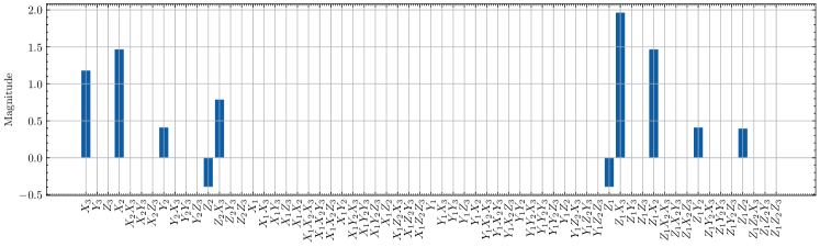
(a) Seed #1

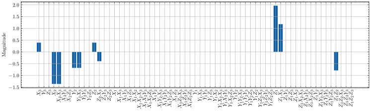
(b) Seed #2

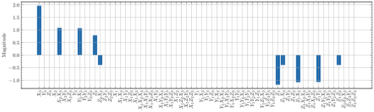
(c) Seed #3

Figure 1: Bar plot of parameter magnitudes for Toffoli gate. We show three different initialisations of initial parameters in (a), (b) and (c). Note how we find many solutions consisting mostly of local fields and a few two-body interactions.

see Fig. 1. For the parametrisation of $U$ given in Equation 3, these directional derivatives are thus given by,

$$\frac{\partial U({\bm{\theta}})}{\partial\theta_{l}}=U({\bm{\theta}})\Omega_{l}({\bm{\theta}}),$$ (6)

where there is an effective generator, $\Omega_{l}$, of the directional derivative in the tangent space for each Lie algebra component $\theta_{l}$.

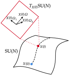
Figure 1: A curve in $\mathrm{SU}(N)$ is parameterised by a continuous variable $t\in\mathbb{R}$. At the point $X(t)$ there is a tangent space of directional derivatives $T_{X(t)}\mathrm{SU}(N)$ with direction $\Omega=\Omega(t)$.

The directional derivatives $\Omega_{l}$ can be calculated classically by using a differentiable programming framework such as JAX [31], which implements a differentiable version of the exponential map. Additionally, one can use Pennylane [32] with the qml.SpecialUnitary class to represent elements of the $\mathrm{SU}(N)$ group [33].

We can equip the smooth manifold of $\mathrm{SU}(N)$ with the metric $g(x,y)=\Tr{x^{\dagger}y}/N$ to turn it into a Riemannian manifold. The metric gives a notion of distance between elements of the $\mathrm{SU}(N)$ group.

A geodesic on $\mathrm{SU}(N)$ is a one-parameter subgroup of the Lie group, $X(t)$, parameterised by $t$ that represents the shortest path between two unitaries. The geodesic between two unitaries $U({\bm{\theta}})$ and $V$ can be constructed as follows. Let $X(t)$ be a one-parameter subgroup in $\mathrm{SU}(N)$ such that $U({\bm{\theta}})X(0)=U({\bm{\theta}})$ and $U({\bm{\theta}})X(1)=V$. The geodesic between $U({\bm{\theta}})$ and $V$ can then be straightforwardly constructed as

$$X(t)=e^{i\Gamma t},$$ (7)

where $\Gamma\in T_{X(t)}\mathrm{SU}(N)$ is the direction of the geodesic on the tangent space given by

$$\Gamma=-i\log(U({\bm{\theta}})^{\dagger}V).$$ (8)

We now introduce the concept of a limited set of Hamiltonian terms – a restriction of the Lie algebra. The basis Pauli words of the Lie algebra, $G_{l}$, are each possible terms of a Hamiltonian. However, Hamiltonians that are physically realisable may not include all possible terms. For example, only one- and two-body interactions may be accessible in an experimental setup. The set of these terms we define as $\mathcal{H}\subset\mathcal{P}$. We can define a binary function over a restricted set,

$$\bar{R}_{\mathcal{H}}(G_{l})=\begin{cases}1,&\text{if $G_{l}$ is in $\mathcal{H}$},\\ 0&\text{otherwise}.\end{cases}$$ (9)

This function can be represented with a diagonal matrix that acts on Lie algebra vectors ${\bm{\theta}}$ and has elements

$$(R_{\mathcal{H}})_{ij}=\delta_{ij}\bar{R}_{\mathcal{H}}(G_{i}).$$ (10)

We use the notation ${\bm{\theta}}$ to refer to unrestricted vectors, and $\bm{\phi}$ to refer to restricted vectors where many components of the vector may have been forced to 0,

$$\bm{\phi}=R_{\mathcal{H}}{\bm{\theta}}.$$ (11)

We will produce multiple sets of parameters via an optimisation algorithm. The initial parameter vector is denoted by $\bm{\phi}^{(0)}$ and subsequent parameter vectors are $\bm{\phi}^{(m)}$ with $0<m\leq M$. The geodesic of the $m$th parameter vector $\bm{\phi}^{(m)}$ is $X^{(m)}(t)$ and its generator is $\Gamma^{(m)}$. The norm of the parameter difference between optimisation steps is the step size,

$$\delta^{(m)}=\|\bm{\delta\theta}^{(m)}\|=\|\bm{\theta}^{(m+1)}-\bm{\theta}^{(m)}\|,$$ (12)

where $\|\cdot\|$ is the Euclidean 2-norm.

Finally, we include a constraint on the Hamiltonians, as discussed in Ref. [25], that can generate a specific $U$ at a fixed time $t=1$. All Hamiltonians that generate $U$ must commute. Given a Hamiltonian of a restricted parameter vector $H(\bm{\phi})$ that generates the quantum gate $U$, we have the necessary condition

$$[H(\bm{\phi}),\log(U)]=0.$$ (13)

This commutator condition further constrains the space of possible Hamiltonians within the restriction $\mathcal{H}$.

III Algorithm

Consider a target unitary $V$ and a parametrised unitary $U(\bm{\phi})=\exp{iH(\bm{\phi})}$, where $\bm{\phi}$ is a restricted vector due to the restriction set $\mathcal{H}\subset\mathcal{P}$ of the generating Hamiltonian $H(\bm{\phi})$. We can use the metric $g$ to define the unitary infidelity

$$\mathcal{I}(\bm{\phi})=1-\frac{1}{N}\Tr{U^{\dagger}(\bm{\phi})V},$$ (14)

which satisfies $\mathcal{I}(\bm{\phi})\in[0,1]$. We aim to minimise $\mathcal{I}(\bm{\phi})$ and find a set of parameters $\bm{\phi}$ that produces a unitary $U(\bm{\phi})$ that is as close as possible to the target $V$. A naive approach that calculates the gradient of Eq. (14) consequently updates the parameters (see App. B) will quickly get stuck in a local minimum and provide a sub-optimal approximation of $V$. Our proposed algorithm adapts this scheme by utilizing geodesic information and gradients on the group manifold to rapidly converge to an accurate solution.

The idea is to use the effective generators $\Omega_{l}(\bm{\phi}^{(m)})$ and the generator of the geodesic $\Gamma^{(m)}$ at $U(\bm{\phi}^{(m)})$ to determine the best way to update the parameters $\bm{\phi}^{(m+1)}=\bm{\phi}^{(m)}+\bm{\delta\phi}^{(m)}$. At each optimisation step, we want to update the parameters such that the resulting unitary $U(\bm{\phi}^{(m+1)})$ is closer to the target unitary $V$. This can be achieved by updating the parameters such that they follow (as closely as possible) the geodesic $X^{(m)}(t)$ towards the target $V$. Consider a small step along the geodesic by $\delta t$,

$$U({\bm{\theta}}^{(m+1)}) =U(\bm{\phi}^{(m)})X(\delta t)$$ (15)

$$=U(\bm{\phi}^{(m)})e^{i\Gamma^{(m)}\delta t}$$ (16)

$$=U(\bm{\phi}^{(m)})+iU(\bm{\phi}^{(m)})\Gamma^{(m)}\delta t+O(\delta t^{2}).$$ (17)

Notice how the geodesic can take us from a unitary given by a restricted parameter vector $\bm{\phi}^{(m)}$ to a unitary with a parameter vector that has components in any direction ${\bm{\theta}}^{(m+1)}$.

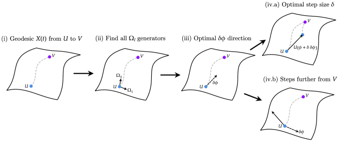
Figure 2: Illustration of the update procedure at step $m$ on the Riemannian manifold of the $\mathrm{SU}(N)$ group: (i) Find the geodesic from current unitary $U(\bm{\phi}^{(m)})$ to the target $V$; (ii) Find all effective generators $\Omega_{j}(\bm{\phi}^{(m)})$; (iii) Solve the convex optimisation problem to give the update step $\bm{\delta\phi}^{(m)}$; (iv.a) Use line search to optimise the update step size $\delta=\|\bm{\delta\phi}^{(m)}\|$; (iv.b) If the solution is currently a local minimum, use the Gram-Schmidt procedure to step away from the local minimum.

A small change in parameter vectors, $|\bm{\delta\phi}|=\delta$, can be expanded as

$$U(\bm{\phi}^{(m+1)}) =U(\bm{\phi}^{(m)}+\bm{\delta\phi}^{(m)})$$ (18)

$$=U(\bm{\phi}^{(m)})+\delta\phi^{(m)}_{j}\frac{\partial U(\bm{\phi}^{(m)})}{\partial\phi_{j}}\bigg{|}_{\bm{\phi}^{(m)}}+O(\delta^{2}),$$ (19)

with $\delta\phi_{j}^{(m)}$ the $j$th element of the vector $\bm{\delta\phi}^{(m)}=\bm{\phi}^{(m+1)}-\bm{\phi}^{(m)}$ and repeated indices are summed over. Up to first order, we find

$$U(\bm{\phi}^{(m+1)})\approx U(\bm{\phi}^{(m)})+U(\bm{\phi}^{(m)})\delta\phi^{(m)}_{j}\Omega_{j}(\bm{\phi}^{(m)}),$$ (20)

where we have used Eq. (6). We want to find the components of $\bm{\delta\phi}^{(m)}$ such that $U(\bm{\phi}^{(m+1)})$ is closer to the target $V$. We can compute all $\Omega_{j}(\bm{\phi}^{(m)})$ using differentiable programming and the geodesic with $\Gamma^{(m)}=-i\log(U(\bm{\phi}^{(m)})^{\dagger}V)$. By comparison of the first order terms in Eqs. (17) and (20), we require

$$\delta\phi^{(m)}_{j}\Omega_{j}(\bm{\phi}^{(m)})=i\Gamma^{(m)},$$ (21)

where repeated index $j$ is summed over and $\delta t$ has been neglected as it only changes the norm of the vector $\bm{\delta\phi}^{(m)}$, which is found later in the algorithm. We can restate the problem of finding $\bm{\delta\phi}$ as finding a linear combination of vectors. First, the geodesic $\Gamma^{(m)}$ and effective generators $\Omega_{l}(\bm{\phi}^{(m)})$ are written as vectors in the Lie algebra

$$\bm{\gamma}^{(m)} =\sum_{j=1}^{N^{2}-1}\Tr{G_{j}\Gamma^{(m)}}\hat{e}_{j},$$ (22)

$$\bm{\omega}^{(m)}_{l} =\sum_{j=1}^{N^{2}-1}\Tr{G_{j}\Omega_{l}(\bm{\phi}^{(m)})}\hat{e}_{j},$$ (23)

where $\hat{e}_{j}$ are basis vectors. We now have a convex optimisation problem known as linear least-squares [34, Section 1.2.2], with no constraints, —l— δϕ^(m)∥∑_j ∀G_j ∈H [δϕ_j^(m) ω^(m)_j] - γ^(m)∥^2, where $\|\cdot\|$ is again the Euclidean 2-norm. Note that many terms in $\bm{\delta\phi}^{(m)}$ are constrained to be 0 because they do not appear in the restriction set $\mathcal{H}$. These constraints do not formally have to appear in the convex optimisation problem because they are not included in the summation. The number of parameters to optimise over is therefore $|\mathcal{H}|$, the cardinality of the set $\mathcal{H}$.

Throughout the algorithm, an additional constraint is applied to the restricted parameter vectors $\bm{\phi}^{(m)}$. The parameter vectors are constrained to satisfy the commutator condition of Eq. (13), which is

$$[H(\bm{\phi}^{(m)}),\log(V)]=0,$$ (24)

for all $m$. This constraint reduces the number of independent $\bm{\phi}$ parameter components, thereby decreasing the number of steps to reach a parameter vector that generates a unitary evolution sufficiently close to the target. Note that it depends on both $V$, and the restricting $\mathcal{H}$ whether commuting parameter constraints can be found. Additionally, since the Hilbert space increases exponentially with the number of qubits, the conditions from this constraint become increasingly difficult to compute. For a low number of qubits, such as $3$ or $4$, it is straightforward to obtain with any symbolic programming language.

A golden section line search on the magnitude of the update vector $\delta^{(m)}$ can then be performed to maximise the update such that the metric $\Tr{U(\bm{\phi}^{(m+1)})^{\dagger}V}$ is largest [35]. However, it is possible to reach local minima, where $\Tr{U(\bm{\phi}^{(m+1)})^{\dagger}V}\leq\Tr{U(\bm{\phi}^{(m)})^{\dagger}V}$. In this case, we generate a random vector $\bm{r}$, apply the restriction $\bm{r}_{\mathcal{H}}=R_{\mathcal{H}}\bm{r}$, and then use the Gram-Schmidt procedure to ensure the vector is orthogonal to the geodesic

$$\bm{\delta\phi}^{(m)}=\bm{r}_{\mathcal{H}}-\frac{\bm{r}_{\mathcal{H}}\cdot\bm{\gamma}^{(m)}}{\|\bm{\gamma}^{(m)}\|^{2}}\bm{\gamma}^{(m)}.$$ (25)

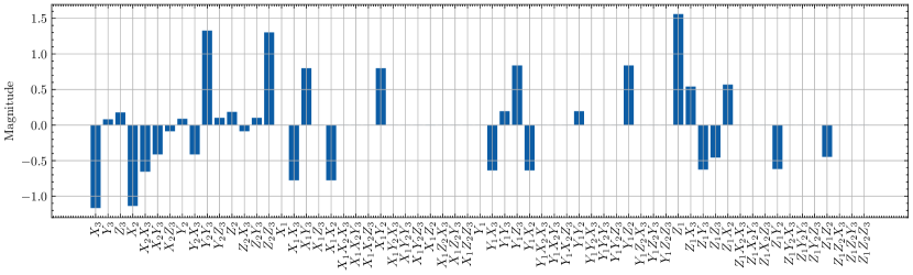
(a) Seed #1

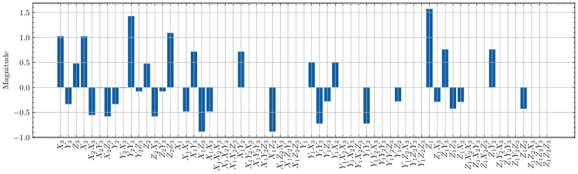
(b) Seed #2

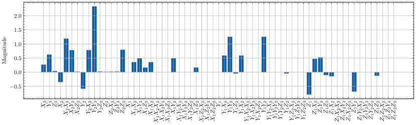
(c) Seed #3

Figure 2: Bar plot of parameter magnitudes for Fredkin gate. We show three different initialisations of initial parameters in (a), (b) and (c). The solutions are much less sparse than for the Toffoli, although some fields have small enough values that can be ignored without much loss of fidelity.

The Gram-Schmidt procedure reduces the chance that the subsequent steps of the algorithm find the same local minima. The steps of the algorithm are depicted in Fig. 2. We can control strength with which we attempt to escape local minima by multiplying the resulting $\bm{\delta\phi}^{(m)}$ with a scalar $\eta$, which is one of the hyperparameters of our algorithm. Finally, we terminate the optimisation when the infidelity is smaller than some desired precision $\varepsilon$. The full algorithm is given in Algorithm 1.

Input: $V$, ${\bm{\theta}},R_{\mathcal{H}},\varepsilon,\eta$

Output: $\bm{\phi}$

Obtain the Jacobian function:

for $l\in(1,\ldots,N^{2}-1$) do

       $dU_{l}({\bm{x}})=\partial_{x_{l}}\mathfrak{Re}[U({\bm{x}})]+i\partial_{x_{l}}\mathfrak{Im}[U({\bm{x}})]$

end for

Define a fidelity function: $F({\bm{\theta}},V)=\Tr{U({\bm{\theta}})^{\dagger}V}/N$

Perform the Hamiltonian restriction: $\bm{\phi}\leftarrow R_{\mathcal{H}}{\bm{\theta}}$

Solve the commutator condition reducing the number of independent $\bm{\phi}$ components: $[H(\bm{\phi}),\log(V)]=0$

Update $\bm{\phi}$ respecting the commutator condition:

while $F(\bm{\phi},V)<1-\varepsilon$ do

       Compute the effective generators at $\bm{\phi}$:

       for $l\in(1,\ldots,N^{2}-1)$ do

            $\Omega_{l}(\bm{\phi})\leftarrow U^{\dagger}(\bm{\phi})dU_{l}({\bm{x}})|_{\bm{\phi}}$

            $\bm{\omega}_{l}\leftarrow\sum_{j=1}^{N^{2}-1}\Tr{G_{j}\Omega_{l}(\bm{\phi})}\hat{e}_{j}$

       end for

      

      Find the geodesic:

       $\Gamma\leftarrow-i\log(U(\bm{\phi})^{\dagger}V)$

       $\bm{\gamma}\leftarrow\sum_{j=1}^{N^{2}-1}\Tr{G_{j}\Gamma(\bm{\phi})}\hat{e}_{j}$

      Minimise$\left(\Big{\|}\sum_{j\forall G_{j}\in\mathcal{H}}\left[\delta\phi_{j}\bm{\omega}_{j}\right]-\bm{\gamma}\Big{\|}^{2}\right)\textrm{ for }\bm{\delta\phi}$

      Maximise$\left(F(\bm{\phi}+\delta\bm{\delta\phi},V)\right)\textrm{ for }\delta$

      if $F(\bm{\phi}+\delta\bm{\delta\phi},V)<F(\bm{\phi},V)$ then

            choose random $\bm{r}$

            $\bm{r}_{\mathcal{H}}\leftarrow R_{\mathcal{H}}\bm{r}$

            $\bm{\delta\phi}\leftarrow\bm{r}_{\mathcal{H}}-\frac{\bm{r}_{\mathcal{H}}\cdot\bm{\gamma}}{\|\bm{\gamma}\|^{2}}\bm{\gamma}$

            $\bm{\phi}\leftarrow\bm{\phi}+\eta\bm{\delta\phi}$

       else

             $\bm{\phi}\leftarrow\bm{\phi}+\delta\bm{\delta\phi}$

       end if

      

end while

Algorithm 1 Geodesic gate design.

IV Numerical experiments

To test the validity of our approach, we construct several quantum gates with the Hamiltonian restriction set $\mathcal{H}_{2-\mathrm{local}}$, which is the set of Pauli words that have only one- and two-body interactions. We see that $|\mathcal{H}_{2-\mathrm{local}}|=9n(n+1)/2+3n=O(\log(N)^{2})$. For this restriction, an optimal solution vector $\bm{\delta\phi}^{(m)}$ can be found for the least-squares problem efficiently in $N$ – in time that scales as $O(\log(N)^{2}N^{4})$.

Throughout the rest of this section, we initialise the parameters as $\bm{\phi}^{(0)}\sim\mathcal{U}(-1,1)$. We set $\eta=1$, which gives a reasonable trade off between exploration and exploitation for the Gram-Schmidt restarting subroutine of our algorithm.

IV.1 Toffoli and Fredkin gate

We first consider two gates that can be combined with single qubit unitaries to form a universal gate set, the Toffoli and Fredkin gate [29]. As a benchmark, we consider the work of Innocenti et al. [24], which attempts to learn a unitary generated by a time-independent Hamiltonian from a set of training data states (see App. A). Additionally, we compare with a simple gradient descent scheme (see App. B). For both the Toffoli and the Fredkin gate, it is possible to further constrain the parameters $\bm{\phi}$ to always ensure that the restricted Hamiltonian commutes with the target. We use the symbolic mathematical package Sympy to find these constraints [36]. In Fig. 3, we show a histogram of the number of steps required to find a high precision Toffoli and Fredkin gate for 1000 random initialisations. Our geodesic algorithm requires significantly fewer steps on average than the other methods. We provide the data to reproduce these figures at [37] and give the parameters for three example solutions for the Toffoli and Fredkin in App. C.

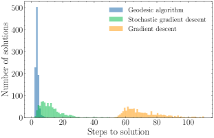
(a) Toffoli

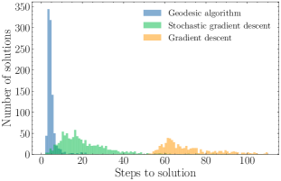
(b) Fredkin

Figure 3: Comparison of the number of steps required before a solution with infidelity less than $\varepsilon=0.001$ is found for: our geodesic algorithm (blue), stochastic gradient descent (SGD) of Ref. [25] (green), and a simple gradient descent optimiser that uses gradients computed with JAX (orange). For all methods, we consider $1000$ random initialisations of the parameters. (a) For the Toffoli gate, both the geodesic algorithm and SGD algorithm find a solution 100% of the time, whereas the JAX gradient descent algorithm finds a solution 98% of the time. (b) For the Fredkin gate, the geodesic algorithm finds a solution 99.3% of the time, the SGD finds a solution 100% of the time. The JAX gradient descent algorithm struggles to find a solution for this gate, with a success rate of only 71.5%.

IV.2 Weight-$k$ Parity checks

In order to build fault-tolerant quantum computers, we will need robust error correction to mitigate the effect of noise in current quantum devices. A widely-used family of quantum error correction codes are so-called stabilizer codes, which rely on measuring syndromes and using the resulting measurement outcome to correct a computation. Of particular interest are surface codes [38], and the toric code [18], which rely on stabilizers that are geometrically local on a two dimensional grid. Crucial to these codes are so called parity checks; error syndromes that can detect flipped bits or phase changes. Here, we consider the unitary corresponding to a weighted $X$ and weighted $Z$ parity check of the form

$$\mathrm{WZ}_{k} =\frac{1}{2}(I^{\otimes k}+Z^{\otimes(k-1)}I+I^{\otimes(k-1)}X-Z^{\otimes(k-1)}X)$$

$$\mathrm{WX}_{k} =\frac{1}{2}(I^{\otimes k}+X^{\otimes(k-1)}I+I^{\otimes(k-1)}X-X^{\otimes k}),$$ (26)

respectively. Here $k$ denotes the size of the check. In Fig. 4, we see that our algorithm is capable of finding accurate approximations for the weight-$k$ parity check unitary, for $k=2,3,4$, which correspond to gates comprising 3, 4, and 5 qubits respectively. Additionally, we found a solution for $k=5$, which is a 6 qubit gate, after approximately $3\times 10^{4}$ steps. Some trajectories in Fig. 4 show the optimisation plateauing for a number of steps, either temporarily or in one case until the maximum step number is reached. Sometimes, the optimisation can repeatedly find a solution that would require Hamiltonian terms which are not in the restriction (e.g. not physical), in order to reach a high fidelity. The Gram-Schmidt procedure provides a method to avoid these infidelity plateaus, however, at the cost of tuning the hyperparameter $\eta$.

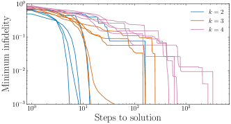
(a) Weight-$k$ $Z$ Parity ($\mathrm{WZ}_{k}$)

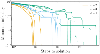
(b) Weight-$k$ $X$ Parity ($\mathrm{WX}_{k}$)

Figure 4: Plot of the minimum infidelity $1-F({\bm{\theta}},V)$ up to each step in the algorithm for weight-$k$ parity checks with $k=\{3,4,5\}$. We show 5 optimisation runs. The steps are shown until the target precision of $0.001$ infidelity is reached. In subsequent steps significantly lower infidelities can be obtained for some trajectories. We do not use the commuting ansatz of Eq. (13) here due to the excessive amount of time it takes to compute the ansatz for larger gates.

V Discussion

The commuting ansatz of Eq. (13) is the requirement that the Hamiltonian at each step $H(\bm{\phi}^{(m)})$ must commute with the principal logarithm of the target $\log(V)$. For a low number of qubits, three or four, we find that the ansatz offers a considerable advantage in the efficiency to discover the solution. Whereas for five or more qubits we find that the solution can be discovered more slowly than by simply ignoring the commuting constraint. The severe restriction imposed by the commuting ansatz on the allowed updates of the parameters prevents the geodesic algorithm from more directly moving towards the target unitary on the manifold.

We find that our geodesic algorithm is significantly more efficient than stochastic gradient descent and gradient descent algorithms for finding a restricted generating Hamiltonian of a desired unitary gate. Gradient descent methods also quickly become unfeasible for larger quantum gates. Our geodesic algorithm takes advantage of how the problem can be described on the Riemannian manifold of $\mathrm{SU}(N)$. We use the fact that the location of the solution on the manifold, the target unitary $V$, is known in advance. Typically, in machine learning, the location of the solution in the phase space is unknown. In these cases, the computation and minimisation of a cost function is required and gradient descent algorithms cannot use information about the location of the target point. In contrast, our geodesic algorithm is aware of the target point and attempts to push the parameters towards that point on the manifold at each step. The effective generators $\Omega_{l}$ provide the necessary information for how the Hamiltonian parameters should be updated in order for the next set of parameters to follow the path of the geodesic to the solution as closely as possible.

Time-independent Hamiltonians generate geodesic curves on the manifold since they are defined by a one-parameter subgroup of $\mathrm{SU}(N)$ parameterised by $t$. These geodesics start at the identity element at $t=0$ and reach the desired unitary evolution at $t=1$. In general, due to the Hamiltonian strengths, these geodesic curves are not necessarily the shortest paths along the manifold, which for a given restriction could be a time-dependent Hamiltonian [39]. Consider a restriction $\mathcal{H}$ and the additional Pauli words $\mathcal{Q}=\mathcal{P}-\mathcal{H}$. The principal generator of a unitary gate generally contains terms from $\mathcal{H}$ and $\mathcal{Q}$. We can define a special commuting case where the specific terms of the principal generator in $\mathcal{Q}$ commute with those in $\mathcal{H}$. In this case, the minimal path along the manifold to generate the desired unitary (given the restriction $\mathcal{H}$) is actually a geodesic generated by a time-independent Hamiltonian [39, Section IV.C.1]. Crucially, the minimal path for the restriction $\mathcal{H}$ is not a quantum circuit with multiple layers of gates or a time-dependent Hamiltonian. Thus, for an initialisation of parameters close to the identity (such that the parameters start small in magnitude), our geodesic algorithm finds the most efficient implementation possible of parity check gates with only one- and two-local Hamiltonian terms.

VI Conclusion

In this work, we have introduced a geodesic algorithm to find time-independent Hamiltonians that implement multi-qubit unitaries. We have only considered the simplest ‘physical’ restriction, using all one- and two-local Hamiltonian terms, but our algorithm could be applied to more constrained Hamiltonians, for example, restricting to Hamiltonian terms that are available on a particular hardware platform. This could lead to applications in quantum hardware, since current experimental platforms for quantum computing offer more complex Hamiltonians than are typically utilised for quantum gates. In fact, the gates implemented at the hardware level are often at most only two-qubit gates. Our geodesic algorithm opens up the possibility of finding time-independent Hamiltonian couplings so that larger, more complex quantum gates can be implemented directly. Additionally, we could combine multiple blocks of time-independent quantum gates together to form more complex gates, where we find the required Hamiltonian couplings of each individual block using our geodesic algorithm. Not only could this lead to less noisy gates, but it could also reduce the total time to run a circuit on the hardware. This is crucial for NISQ applications where we have a limited coherence time and gives the significant advantage of increasing the clock speed for fault-tolerant quantum computation.

VII Acknowledgements

DL acknowledges support from the EPSRC Centre for Doctoral Training in Delivering Quantum Technologies, grant ref. EP/S021582/1. JC acknowledges support from the Natural Sciences and Engineering Research Council (NSERC), the Shared Hierarchical Academic Research Computing Network (SHARCNET), Compute Canada, and the Canadian Institute for Advanced Research (CIFAR) AI chair program. Resources used in preparing this research were provided, in part, by the Province of Ontario, the Government of Canada through CIFAR, and companies sponsoring the Vector Institute www.vectorinstitute.ai/#partners.

VIII Competing interests

DL, RW, and SB declare a relevant patent application: United Kingdom Patent Application No. 2400342.8.

Supplemental Material

A Stochastic Gradient Descent

Here, we summarise the stochastic gradient descent algorithm from Ref. [24] which is used for the numerical results in the main text.

We consider the same setup as in the main text, with $\mathcal{H}\subset\mathcal{P}$ the restricted set of Pauli strings and $\bm{\phi}=R_{\mathcal{H}}{\bm{\theta}}$ the parameters of the restricted Hamiltonian. Instead of considering the direct minimisation of the unitary infidelity of Eq. (14), we can consider the average state infidelity over a set of $d$ states $\mathcal{D}=\{\ket{\psi_{i}}\}^{d}$,

$$\mathcal{I}_{\mathcal{D}}(\bm{\phi})=1-\frac{1}{d}\sum_{i}^{d}\absolutevalue{\bra{\psi_{i}}U^{\dagger}(\bm{\phi})V\ket{\psi_{i}}}^{2}$$ (A1)

Minimizing the function $\mathcal{I}_{\mathcal{D}}(\bm{\phi})$ for some finite set of states is an example of supervised learning [40]. Note that if $\mathcal{D}=\{\ket{b_{i}}\}^{N}$ is the set of all computational basis states, where $\ket{b_{i}}$ is a computational basis state corresponding to bit $i$, then $\mathcal{I}_{\mathcal{D}}(\bm{\phi})\equiv\mathcal{I}(\bm{\phi})$. The cost of evaluating $\mathcal{I}_{\mathcal{D}}(\bm{\phi})$ is $O(d\times N)$ compared to $O(N^{2})$ for $\mathcal{I}(\bm{\phi})$, hence it is a cheaper method of estimating the infidelity. Additionally, the stochasticity of the optimisation could be useful in escaping from local minima.

To minimise the cost in Eq. (A1) in practice one can perform a stochastic gradient descent algorithm, which uses the gradient over randomly sampled elements of a data set to minimise a cost function. We randomly initialise the parameters of our model $\bm{\phi}^{(0)}\sim\mathcal{U}(-1,1)$. At the $m$th step of the optimisation, we create a data set $\mathcal{D}^{(m)}=\{\ket{\psi_{i}^{(m)}}\}^{d_{\mathrm{train}}}$ that is randomly sampled from the Haar measure. Then, we obtain the gradients with respect to $\bm{\phi}$ using the automatic differentiation framework Theano [41]. We update the parameters of the model with a standard gradient descent update step with an initial learning rate $\lambda^{(0)}=1$. Throughout the optimisation, the learning rate is decayed as

$$\lambda^{(m+1)}=\frac{\lambda^{(0)}}{1+\kappa\times m}$$ (A2)

at each step $m$, where $\kappa$ is defined as the gradient decay rate. In the spirit of machine learning, we keep a fixed validation set of states $\mathcal{D}_{\mathrm{val}}=\{\ket{\psi_{i}^{(m)}}\}^{d_{\mathrm{test}}}$ to track the performance of the model during the optimisation. If the test set is large enough, this should give an accurate estimate of the true infidelity. For the experiments in the main text, we make use of the hyperparameters in Table 1 which are are the same as in Ref. [24].

Name	Value
${d_{\mathrm{train}}}$	200
${d_{\mathrm{test}}}$	100
Gradient decay rate $\kappa$	0.005

Table 1: Stochastic gradient descent hyperparameters

B Gradient Descent

Here we summarise the gradient descent algorithm which is used for the numerical results in the main text.

A simple algorithm to find the generator of a target unitary $V$ can be described as follows. We consider the same setup as in the main text, with $\mathcal{H}\subset\mathcal{P}$ the restricted set of Pauli strings and $\bm{\phi}=R_{\mathcal{H}}{\bm{\theta}}$ the parameters of the restricted Hamiltonian. We consider the minimisation of the infidelity in Eq. (14) and attempt to solve this optimisation problem via gradient descent. At each step $m$ of the optimisation, we obtain the gradients

$$\frac{\partial U(\bm{\phi}^{(m)})}{\partial\phi_{j}}\bigg{|}_{\bm{\phi}^{(m)}}=U(\bm{\phi})\Omega_{j}(\bm{\phi})$$ (B1)

via automatic differentiation with Jax [31], since the matrix exponential jax.scipy.linalg.expm is supported as a differentiable function. Once we obtain the gradients, we use ADAM [42] to update the parameters $\bm{\phi}$. For the results in the main text we used a learning rate of $\lambda=10^{-1}$. We do not include the commutator condition of Eq. (13), nor do we use a line search to find the optimal step size.

C Parameters

In this section we show three sets of parameters for the Toffoli and Fredkin gate found by our algorithm. For both gates, we initialise the parameters close to the identity, which in practice helps with finding sparse solutions where many of the Hamiltonian terms have coefficients close to zero. All solutions shown here have an error of $\varepsilon<10^{-3}$.

I Toffoli

II Fredkin

References

- Barenco et al. [1995] A. Barenco, C. H. Bennett, R. Cleve, D. P. DiVincenzo, N. Margolus, P. Shor, T. Sleator, J. Smolin, and H. Weinfurter, Elementary gates for quantum computation, Physical Review A 52, 3457 (1995), arXiv:quant-ph/9503016.
- Nielsen and Chuang [2010] M. A. Nielsen and I. L. Chuang, Quantum Computation and Quantum Information: 10th Anniversary Edition (2010), iSBN: 9780511976667 Publisher: Cambridge University Press.
- Porras and Cirac [2004] D. Porras and J. I. Cirac, Effective Quantum Spin Systems with Trapped Ions, Physical Review Letters 92, 207901 (2004), publisher: American Physical Society.
- Kim et al. [2011] K. Kim, S. Korenblit, R. Islam, E. E. Edwards, M.-S. Chang, C. Noh, H. Carmichael, G.-D. Lin, L.-M. Duan, C. C. J. Wang, J. K. Freericks, and C. Monroe, Quantum simulation of the transverse Ising model with trapped ions, New Journal of Physics 13, 105003 (2011), publisher: IOP Publishing.
- Blatt and Roos [2012] R. Blatt and C. F. Roos, Quantum simulations with trapped ions, Nature Physics 8, 277 (2012), number: 4 Publisher: Nature Publishing Group.
- Wall et al. [2017] M. L. Wall, A. Safavi-Naini, and A. M. Rey, Boson-mediated quantum spin simulators in transverse fields: $XY$ model and spin-boson entanglement, Physical Review A 95, 013602 (2017), publisher: American Physical Society.
- Kiely and Freericks [2017] T. G. Kiely and J. K. Freericks, Relationship between the transverse-field Ising model and the XY model via the rotating-wave approximation 10.1103/PhysRevA.97.023611 (2017).
- Lewis et al. [2022] D. Lewis, L. Banchi, Y. H. Teoh, R. Islam, and S. Bose, Ion Trap Long-Range XY Model for Quantum State Transfer and Optimal Spatial Search (2022), arXiv:2206.13685 [quant-ph].
- Morgado and Whitlock [2021] M. Morgado and S. Whitlock, Quantum simulation and computing with Rydberg-interacting qubits, AVS Quantum Science 3, 023501 (2021).
- Preskill [2018] J. Preskill, Quantum Computing in the NISQ era and beyond, Quantum 2, 79 (2018), publisher: Verein zur Forderung des Open Access Publizierens in den Quantenwissenschaften.
- Chen et al. [2022] S. Chen, J. Cotler, H.-Y. Huang, and J. Li, The Complexity of NISQ (2022), arXiv:2210.07234 [quant-ph].
- Cerezo et al. [2021] M. Cerezo, A. Arrasmith, R. Babbush, S. C. Benjamin, S. Endo, K. Fujii, J. R. McClean, K. Mitarai, X. Yuan, L. Cincio, and P. J. Coles, Variational Quantum Algorithms, Nature Reviews Physics 3, 625 (2021), arXiv:2012.09265 [quant-ph, stat].
- Linke et al. [2017] N. M. Linke, D. Maslov, M. Roetteler, S. Debnath, C. Figgatt, K. A. Landsman, K. Wright, and C. Monroe, Experimental Comparison of Two Quantum Computing Architectures, Proceedings of the National Academy of Sciences 114, 3305 (2017), arXiv:1702.01852 [quant-ph].
- Li et al. [2018] M. Li, D. Miller, and K. R. Brown, Direct measurement of Bacon-Shor code stabilizers, Physical Review A 98, 050301 (2018), arXiv:1804.01127 [quant-ph].
- Hastings and Haah [2021] M. B. Hastings and J. Haah, Dynamically Generated Logical Qubits, Quantum 5, 564 (2021), publisher: Verein zur Förderung des Open Access Publizierens in den Quantenwissenschaften.
- Bravyi et al. [2013] S. Bravyi, G. Duclos-Cianci, D. Poulin, and M. Suchara, Subsystem surface codes with three-qubit check operators, Quantum Information & Computation 13, 963 (2013).
- Kitaev [1997] A. Y. Kitaev, Quantum computations: algorithms and error correction, Russian Mathematical Surveys 52, 1191 (1997), publisher: IOP Publishing.
- Bravyi and Kitaev [1998] S. B. Bravyi and A. Y. Kitaev, Quantum codes on a lattice with boundary (1998), arXiv:quant-ph/9811052.
- Kitaev [2003] A. Y. Kitaev, Fault-tolerant quantum computation by anyons, Annals of Physics 303, 2 (2003).
- Chamberland et al. [2020] C. Chamberland, A. Kubica, T. J. Yoder, and G. Zhu, Triangular color codes on trivalent graphs with flag qubits, New Journal of Physics 22, 023019 (2020), publisher: IOP Publishing.
- Srivastava et al. [2022] B. Srivastava, A. F. Kockum, and M. Granath, The XYZ$^2$ hexagonal stabilizer code, Quantum 6, 698 (2022), publisher: Verein zur Förderung des Open Access Publizierens in den Quantenwissenschaften.
- Benjamin and Bose [2003] S. C. Benjamin and S. Bose, Quantum Computing with an Always-On Heisenberg Interaction, Physical Review Letters 90, 4 (2003), publisher: American Physical Society.
- Banchi et al. [2016] L. Banchi, N. A. Pancotti, and S. Bose, Quantum gate learning in qubit networks: Toffoli gate without time-dependent control, npj Quantum Information 2, 1 (2016), publisher: Nature Partner Journals.
- Innocenti et al. [2018] L. Innocenti, L. Banchi, S. Bose, A. Ferraro, and M. Paternostro, Approximate supervised learning of quantum gates via ancillary qubits, International Journal of Quantum Information 16, 10.1142/S021974991840004X (2018), publisher: World Scientific Publishing Co. Pte Ltd.
- Innocenti et al. [2020] L. Innocenti, L. Banchi, A. Ferraro, S. Bose, and M. Paternostro, Supervised learning of time-independent Hamiltonians for gate design 10.1088/1367-2630/ab8aaf (2020), iSBN: 82.169.190.85.
- Eloie et al. [2018] L. Eloie, L. Banchi, and S. Bose, Quantum arithmetics via computation with minimized external control: The half-adder, Physical Review A 97, 062321 (2018), publisher: American Physical Society.
- Majumder et al. [2022] A. Majumder, D. Lewis, and S. Bose, Variational Quantum Circuits for Multi-Qubit Gate Automata (2022), arXiv:2209.00139 [quant-ph].
- Nielsen [2005] M. A. Nielsen, A geometric approach to quantum circuit lower bounds (2005), arXiv:quant-ph/0502070.
- Nielsen et al. [2006] M. A. Nielsen, M. R. Dowling, M. Gu, and A. C. Doherty, Quantum Computation as Geometry, Science 311, 1133 (2006), publisher: American Association for the Advancement of Science.
- Bhattacharyya et al. [2020] A. Bhattacharyya, P. Nandy, and A. Sinha, Renormalized Circuit Complexity, Physical Review Letters 124, 101602 (2020), publisher: American Physical Society.
- Bradbury et al. [2018] J. Bradbury, R. Frostig, P. Hawkins, M. J. Johnson, C. Leary, D. Maclaurin, G. Necula, A. Paszke, J. VanderPlas, S. Wanderman-Milne, and Q. Zhang, JAX: composable transformations of Python+NumPy programs (2018).
- Bergholm et al. [2018] V. Bergholm, J. Izaac, M. Schuld, C. Gogolin, S. Ahmed, V. Ajith, M. S. Alam, G. Alonso-Linaje, B. AkashNarayanan, A. Asadi, et al., Pennylane: Automatic differentiation of hybrid quantum-classical computations, arXiv preprint arXiv:1811.04968 (2018).
- Wiersema et al. [2023] R. Wiersema, D. Lewis, D. Wierichs, J. Carrasquilla, and N. Killoran, Here comes the $\mathrm{SU}(N)$: multivariate quantum gates and gradients (2023), arXiv:2303.11355 [quant-ph].
- Boyd and Vandenberghe [2004] S. P. Boyd and L. Vandenberghe, Convex optimization (Cambridge university press, 2004).
- Kiefer [1953] J. Kiefer, Sequential minimax search for a maximum, Proceedings of the American mathematical society 4, 502 (1953).
- Meurer et al. [2017] A. Meurer, C. P. Smith, M. Paprocki, O. Čertík, S. B. Kirpichev, M. Rocklin, A. Kumar, S. Ivanov, J. K. Moore, S. Singh, T. Rathnayake, S. Vig, B. E. Granger, R. P. Muller, F. Bonazzi, H. Gupta, S. Vats, F. Johansson, F. Pedregosa, M. J. Curry, A. R. Terrel, v. Roučka, A. Saboo, I. Fernando, S. Kulal, R. Cimrman, and A. Scopatz, Sympy: symbolic computing in python, PeerJ Computer Science 3, e103 (2017).
- Lewis and Wiersema [2023] D. Lewis and R. Wiersema, A Geodesic Algorithm for Unitary Gate Design with Time-Independent Hamiltonians (2023), https://github.com/dyylan/geodesic_design.
- Fowler et al. [2012] A. G. Fowler, M. Mariantoni, J. M. Martinis, and A. N. Cleland, Surface codes: Towards practical large-scale quantum computation, Physical Review A 86, 032324 (2012), publisher: American Physical Society.
- Dowling and Nielsen [2008] M. R. Dowling and M. A. Nielsen, The geometry of quantum computation, Quantum Information & Computation 8, 861 (2008).
- Murphy [2022] K. P. Murphy, Probabilistic Machine Learning: An introduction (MIT Press, 2022).
- Al-Rfou et al. [2016] R. Al-Rfou, G. Alain, A. Almahairi, C. Angermueller, D. Bahdanau, N. Ballas, F. Bastien, J. Bayer, A. Belikov, A. Belopolsky, et al., Theano: A python framework for fast computation of mathematical expressions, arXiv e-prints , arXiv (2016).
- Kingma and Ba [2015] D. P. Kingma and J. Ba, Adam: A method for stochastic optimization, in 3rd International Conference on Learning Representations, ICLR 2015, San Diego, CA, USA, May 7-9, 2015, Conference Track Proceedings, edited by Y. Bengio and Y. LeCun (2015).