Learning physics-based reduced models from data for the Hasegawa-Wakatani equations

Abstract

This paper focuses on the construction of non-intrusive Scientific Machine Learning (SciML) Reduced-Order Models (ROMs) for nonlinear, chaotic plasma turbulence simulations. In particular, we propose using Operator Inference (OpInf) to build low-cost physics-based ROMs from data for such simulations. As a representative example, we focus on the Hasegawa-Wakatani (HW) equations used for modeling two-dimensional electrostatic drift-wave plasma turbulence. For a comprehensive perspective of the potential of OpInf to construct accurate ROMs for this model, we consider a setup for the HW equations that leads to the formation of complex, nonlinear, and self-driven dynamics, and perform two sets of experiments. We first use the data obtained via a direct numerical simulation of the HW equations starting from a specific initial condition and train OpInf ROMs for predictions beyond the training time horizon. In the second, more challenging set of experiments, we train ROMs using the same dataset as before but this time perform predictions for six other initial conditions. Our results show that the OpInf ROMs capture the important features of the turbulent dynamics and generalize to new and unseen initial conditions while reducing the evaluation time of the high-fidelity model by up to five orders of magnitude in single-core performance. In the broader context of fusion research, this shows that non-intrusive SciML ROMs have the potential to drastically accelerate numerical studies, which can ultimately enable tasks such as the design and real-time control of optimized fusion devices.

1 Introduction

Recent advances in computer architecture, algorithms, and software implementations allow the simulation of complex phenomena – such as turbulent transport in fusion devices – with unprecedented accuracy. The standard paradigm in this context is to use supercomputers to perform a small set of high-fidelity simulations for each study. A possible alternative is provided by Reduced-Order Models (ROMs) [3]. Here, the idea is to construct computationally cheap but sufficiently accurate approximations of high-fidelity models with the goal of replacing them for tasks such as simulations over longer time horizons or important many-query tasks such as uncertainty quantitation, control, and design optimization.

In recent years, Scientific Machine Learning (SciML) developed tools for building reduced models for complex applications by combining the rigour of physics-based modeling with the convenience of data-driven learning. In essence, given data stemming from numerical simulations, experimental measurements, or both, SciML constructs approximations by embedding physics principles into the learning problem.

In the present paper, we focus on constructing SciML ROMs for complex plasma turbulence models with the goal of showing that such ROMs can provide predictions with sufficient accuracy while drastically reducing the computational cost of the high-fidelity simulation code. In particular, we focus on Operator Inference (OpInf) [29]. OpInf is a SciML approach for learning physics-based reduced models from data for models with polynomial structure [29]. More general types of nonlinearities can be considered as well by making use of lifting transformations [24, 31] that expose (sometimes only approximate) polynomial structure in the lifted governing equations. OpInf was used to construct ROMs for complex applications such as reactive flows in rocket engines [9, 30, 34], solar wind predictions in space weather applications [20], solidification simulations [23], and chaotic systems [6] such as Lorenz 96 and the Kuramoto-Sivashinsky equations. Extensions include using filtering [10] and roll-outs [36] to handle noisy, scarce, and low-quality data, and quadratic manifolds [12] to address some of the challenges in problems with complex dynamics.

The plasma turbulence model under consideration is given by the Hasegawa-Wakatani (HW) equations [18]. These equations model two-dimensional electrostatic drift-wave turbulence in a slab geometry and have been studied extensively in plasma physics research [5, 26, 28]. The dynamics of these equations were analyzed using Proper Orthogonal Decomposition (POD) [4], a classical approach for constructing linear ROMs, in Refs. [33, 39]. Ref. [14] constructed ROMs for the linearized HW equations using balanced truncation, whereas neural network approximations were used for closure modeling in the context of Large Eddy Simulations in Ref. [16] and for particle flux prediction in Ref. [19]. Further ROM studies related to plasma physics beyond the HW equations include Ref. [7, 11, 25, 35] which used dynamic mode decomposition (DMD) and Proper Orthogonal Decomposition (POD) for analyzing plasma dynamics, Refs. [8, 22] which used these methods for constructing ROMs for predictions beyond their training time horizon, and Ref. [21] which used neural networks to approximate quantities of interest (QoIs) such as the particle flux. Nevertheless, constructing ROMs for plasma turbulence simulations is still in the early stages due to the complexity associated to the nonlinear dynamics of these simulations across multiple spatial and temporal scales.

In this paper, we take a step forward in this direction and propose using OpInf for constructing computationally cheap SciML ROMs for key QoIs in the HW equations, namely the time traces for the particle flux and resistive dissipation. These two QoIs represent the dominant energy source and sink in the HW model and are therefore ubiquitous for assessing turbulent transport. Since their time evolution is complex and exhibits a chaotic behaviour, constructing ROMs of any kind for this problem is non-trivial. We therefore do not seek OpInf ROMs that provide point-wise accurate predictions and instead follow standard practices from plasma physics research and aim to construct ROMs that provide statistically accurate predictions. For a more comprehensive understanding of the potential of OpInf to construct statistically accurate and robust ROMs, we perform two sets of experiments using a training data set stemming from a Direct Numerical Simulation (DNS) of the HW equations. In the first experiment we use this data set to train ROMs for predictions beyond the training horizon while in the second experiment we train ROMs for predictions for different initial conditions. We note that to the best of our knowledge, this represents one of the first studies in which SciML ROMs are considered for the HW equations.

The remainder of the paper is structured as follows. Section 2 summarizes the HW equations and the relevant QoI, as well as the setup for numerical simulations. Section 3 presents the steps to construct physics-based data-driven ROMs via OpInf for the HW system. Section 4 presents our numerical results and discusses our findings. Section 5 concludes the paper.

2 Modeling plasma turbulence via the Hasegawa-Wakatani equations

This section summarizes the HW equations for modeling two-dimensional electrostatic drift-wave plasma turbulence. Section 2.1 provides the physics background. Section 2.2 presents the HW equations, followed by Section 2.3, which presents the two most relevant QoIs. Section 2.4 provides the setup used to solve the HW system numerically via DNS.

2.1 Physics background

The HW equations represent a nonlinear two-dimensional fluid model for drift-wave turbulence in magnetized plasmas [5, 18, 37]. They model the fluctuations of the plasma density and potential in a plane perpendicular to the magnetic field and in the presence of a background density gradient.

The modeling assumptions are as follows. The magnetic field is assumed to be homogeneous and constant in the $z$-direction. In addition, the background density $n_{0}(x,y)=n_{0}(x)$ is non-uniform in the $x$-direction and has a constant equilibrium density scale $L_{n}=|\partial_{x}\log n_{0}|^{-1}$. The gradient in the background density transports particles in the positive $x$-direction, which continuously introduces energy and drives the turbulent transport in the system.

The spatial and temporal coordinates as well as the fields are rescaled to be dimensionless. Following [5], let $\bar{x}$, $\bar{y}$, and $\bar{t}$ represent the two spatial and time coordinates in Gaussian Centimeter-Gram-Second (CGS) units. The inverse of the sound radius $\rho_{s}=c_{s}/\omega_{ci}$ scales the spatial coordinates to $x$ and $y$ as $x=\bar{x}/\rho_{s}$ and $y=\bar{y}/\rho_{s}$, respectively, while the electron drift frequency $\omega_{de}=c_{s}/L_{n}$ scales the time $\bar{t}$ as $t=\bar{t}\omega_{de}$. Here, $c_{s}=\sqrt{T_{e}/m_{i}}$ denotes the ion sound speed and $\omega_{ci}=eB_{0}/(m_{i}c)$ is the ion cyclotron frequency, where $T_{e}$ is the electron temperature, $m_{i}$ represents the ion mass, $e$ is the electric charge, $B_{0}$ is the magnetic field, and $c$ is the speed of light. Lastly, the normalized density and potential fluctuations $\tilde{n}$ and $\tilde{\phi}$ are obtained from the original fields $\bar{n}$ and $\bar{\phi}$ as

$$\tilde{n}=\frac{\bar{n}}{n_{0}}\frac{L_{n}}{\rho_{s}}\quad\text{and}\quad\tilde{\phi}=\frac{e\bar{\phi}}{T_{e}}\frac{L_{n}}{\rho_{s}}.$$ (1)

2.2 The Hasegawa-Wakatani equations

The HW equations describe the time evolution of density $\tilde{n}$ and potential $\tilde{\phi}$ fluctuations in a two-dimensional slab geometry of size $L\times L$ under the influence of the background magnetic field and the background density gradient. They read

$$\begin{cases}{\partial_{t}}\nabla^{2}\tilde{\phi}&=c_{1}(\tilde{\phi}-\tilde{n})-\{\tilde{\phi},\nabla^{2}\tilde{\phi}\}+\nu\nabla^{2N}\tilde{\phi}\\ {\partial_{t}}\tilde{n}&=c_{1}(\tilde{\phi}-\tilde{n})-\{\tilde{\phi},\tilde{n}\}-\partial_{y}\tilde{\phi}+\nu\nabla^{2N}\tilde{n},\end{cases}$$ (2)

where $\nabla^{2}\tilde{\phi}$ is the vorticity and $\{f,g\}:=\partial_{x}f\partial_{y}g-\partial_{y}f\partial_{x}g$ denotes the Poisson bracket of $f$ and $g$. The adiabaticity parameter $c_{1}>0$ controls how fast the electric potential reacts to changes in the density and it exerts a significant impact on the dynamics of these equations. In the limit $c_{1}\to\infty$, the potential reacts instantaneously to changes in the density and the model reduces to the Hasegawa-Mima equation [17]. In the other extreme, when $c_{1}\to 0$, the density and potential are decoupled and the model reduces to the Navier-Stokes equations [5]. Lastly, the hyperdiffusion terms $\nabla^{2N}$ are introduced into the model to prevent energy accumulation at the grid scale, with the hyperdiffusivity coefficient $\nu$ controlling the amount of dissipated energy. Here, we assume periodic boundary conditions in both spatial directions. After initialization, the dynamics undergo a transient phase in which drift-waves dominate the dynamics, and the energy grows exponentially. The dynamics subsequently enter the turbulent phase, where nonlinearities come into play and turbulent transport dominates.

2.3 Energy balance and quantities of interest

The gradient in the background density continuously transports particles from the background density $n_{0}$ to the fluctuating density $\tilde{n}$, therefore driving the turbulent dynamics. The particle flux $\Gamma_{n}$ measures the rate at which particles enter the system and is defined as

$$\Gamma_{n}(t)=-\frac{1}{L^{2}}\int\!\mathrm{d}\mathbf{x}\;\;\tilde{n}(t,\mathbf{x})\partial_{y}\tilde{\phi}(t,\mathbf{x}),$$ (3)

where $\mathrm{d}\mathbf{x}=\mathrm{d}x\,\mathrm{d}y$ and $\mathbf{x}=(x,y)$. At the same time, energy is resistively dissipated. Resistive dissipation constitutes the main energy sink and is quantified by $\Gamma_{c}$ as

$$\Gamma_{c}(t)=\frac{c_{1}}{L^{2}}\int\!\mathrm{d}\mathbf{x}\;\left(\tilde{n}(t,\mathbf{x})-\tilde{\phi}(t,\mathbf{x})\right)^{2}.$$ (4)

These two quantities represent the dominant energy source and sink in the HW model. In the turbulent phase, nonlinear saturation occurs when the particle flux and the resistive dissipation rate balance. Given their importance for assessing turbulent transport in the HW equations, $\Gamma_{n}$ and $\Gamma_{c}$ represent the QoIs in our numerical experiments. Our main goal in the present paper is to construct low-cost data-driven ROMs that can accurately and reliably predict them.

2.4 Numerical setup for solving the Hasegawa-Wakatani equations

We solve the HW equations (2) using DNS following the setup from Ref. [16]. The size of the $2$D slab geometry domain is $L\times L=(2\pi/k_{0})^{2}$ with $k_{0}=0.15$. The equations are solved over the (normalized) time horizon $[0,1\,000]$ in increments of $\delta_{t}=0.025$. The initial conditions are instances of a standard two-dimensional Gaussian random field.

The $2$D domain is discretized using an equidistant grid comprising $N_{x}=512\times 512=262\,144$ spatial degrees of freedom. Since we have $N_{s}=2$ state variables, the total number of degrees of freedom is therefore $N_{\mathrm{state}}=N_{s}\times N_{x}=524\,288$. In addition, we denote $N_{\mathrm{out}}=2$ for the two output QoIs.

The Poisson brackets are discretized using a $4$th order Arakawa scheme [2]. The remaining spatial derivatives, including the derivative in (3), are discretized using $2$nd order finite differences, whereas the two QoIs (3) and (4) are approximated using the trapezoidal rule. The time iterations consist of two steps. First, the HW equations (2) are solved using the explicit $4$th order Runge-Kutta method [32] resulting in the density $\tilde{n}$ and vorticity $\nabla^{2}\tilde{\phi}$. In the second step, the Poisson equation $\nabla^{2}\tilde{\phi}$ is solved using spectral methods to compute $\tilde{\phi}$. A reference implementation is available at https://github.com/the-rccg/hw2d [15].

The adiabaticity parameter is set to $c_{1}=1$ and the diffusivity parameter is $\nu=10^{-6}$ with hyperdiffusion order $N=3$. With the presented setup, one high-fidelity DNS takes about eight hours on a single core of an Intel(R) Xeon(R) 6148 CPU. This setup, and the value of $c_{1}$ in particular, leads to the formation of complex, nonlinear and self-driven dynamics, which makes the construction of predictive ROMs of any kind challenging. Ref. [16] observed that the turbulent phase begins around $t=300$. In our experiments, we will focus on the time horizon starting at $t_{\text{init}}=500$ to ensure that the turbulent dynamics are fully developed. Figure 1 plots example density, potential, and vorticity fields in the turbulent phase. Note that due to the term $c_{1}(\tilde{\phi}-\tilde{n})$ in (2), the density and potential are similar on the large scales but differ at the small scales. Furthermore, Figure 2 plots examples of these two QoIs from initialization to nonlinear saturation over time horizon $[0,1\,000]$.

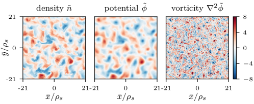
Figure 1: Example density $\tilde{n}$, potential fluctuations $\tilde{\phi}$, and normalized vorticity $\nabla^{2}\tilde{\phi}$ in the turbulent phase.

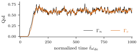
Figure 2: Example particle flux $\Gamma_{n}$ and resistive dissipation rate $\Gamma_{c}$ from initialization to nonlinear saturation up to $t=1\,000$.

3 Learning physics-based data-driven reduced models for the Hasegawa-Wakatani system via Operator Inference

In this section, we propose using OpInf to construct computationally cheap data-driven ROMs for the QoI in the HW equations. Section 3.1 summarizes the OpInf setup followed by Section 3.2 which presents the steps to construct OpInf ROMs. We end with Section 3.3 where we discuss how we assess the accuracy of the resulting OpInf ROM solutions.

3.1 Preliminaries

We first identify the structure of the governing equations. In the context of OpInf, the governing equations are written in semi-discrete form after discretizing the underlying partial differential equation (PDE) model in space. For the HW equations, the spatial discretization of the state equations (2) together with the estimation of the QoIs (3) and (4) using the setup summarized in Section 2.4, allows writing the governing equations in semi-discrete form as a quadratic system of coupled equations over time horizon $[500,t_{\text{final}}]$ with $t_{\text{final}}$ denoting the end of the time horizon,

$$\dot{\mathbf{q}}(t) =\mathbf{A}\mathbf{q}(t)+\mathbf{H}(\mathbf{q}(t)\otimes\mathbf{q}(t))$$ (5a)

$$\mathbf{y}(t) =\mathbf{C}\mathbf{q}(t)+\mathbf{G}(\mathbf{q}(t)\otimes\mathbf{q}(t)),$$ (5b)

where $\mathbf{q}(t)=\begin{pmatrix}\tilde{\mathbf{n}}(t)&\tilde{\mathbf{\phi}}(t)\end{pmatrix}^{\top}\in\mathbb{R}^{N_{\mathrm{state}}}$ denotes the spatially discretized state variables at time $t$ and $\mathbf{y}(t)=\begin{pmatrix}\Gamma_{n}(t)&\Gamma_{c}(t)\end{pmatrix}^{\top}\in\mathbb{R}^{N_{\mathrm{out}}}$ the corresponding outputs, $\mathbf{A}\in\mathbb{R}^{N_{\mathrm{state}}\times N_{\mathrm{state}}}$ and $\mathbf{H}\in\mathbb{R}^{N_{\mathrm{state}}\times N_{\mathrm{state}}^{2}}$ denote the linear and quadratic state operators, whereas $\mathbf{C}\in\mathbb{R}^{N_{\mathrm{out}}\times N_{\mathrm{state}}}$ and $\mathbf{G}\in\mathbb{R}^{N_{\mathrm{out}}\times N_{\mathrm{state}}^{2}}$ are the linear and quadratic output operators, with $N_{\mathrm{state}}=524\,288$ and $N_{\mathrm{out}}=2$. The initial condition in (5a) is the high-dimensional state solution at $t=500$. We refer to (5) as the HW system.

We consider the setup where we are given a training dataset over a time horizon $[500,t_{\text{train}}]$ with $t_{\text{train}}\leq t_{\text{final}}$ obtained by solving the HW system using the setup from Section 2.4 and recording the corresponding state vectors $\mathbf{q}_{i}=\mathbf{q}(t_{i})$ and outputs $\mathbf{y}_{i}=\mathbf{y}(t_{i})$ at $n_{t}$ time instants $t_{i}\in[500,t_{\text{train}}]$. The two sets of solutions are assembled into a snapshot matrix $\mathbf{Q}\in\mathbb{R}^{N_{\mathrm{state}}\times n_{t}}$ and an output matrix $\mathbf{Y}\in\mathbb{R}^{N_{\mathrm{out}}\times n_{t}}$,

$$\mathbf{Q}=\begin{bmatrix}|&|&&|\\ \mathbf{q}_{1}&\mathbf{q}_{2}&\ldots&\mathbf{q}_{n_{t}}\\ |&|&&|\end{bmatrix}\quad\text{and}\quad\mathbf{Y}=\begin{bmatrix}|&|&&|\\ \mathbf{y}_{1}&\mathbf{y}_{2}&\ldots&\mathbf{y}_{n_{t}}\\ |&|&&|\end{bmatrix},$$

with the state vectors $\mathbf{q}_{i}$ and outputs $\mathbf{y}_{i}$ as their respective $i$th columns. Given $\mathbf{Q}$ and $\mathbf{Y}$, our goal is to construct OpInf ROMs that provide accurate output predictions.

3.2 Learning physics-based data-driven reduced models via Operator Inference

OpInf is a SciML approach that combines the perspectives of physics-based modeling with data-driven learning to non-intrusively construct computationally cheap ROMs of systems with polynomial nonlinearities from data [29]. For more general types of nonlinearities, lifting transformations [31] can be used to expose (sometimes only approximate) polynomial structure in the lifted governing equations. OpInf requires two main ingredients: knowledge about the structure of the governing equations and a training data set to construct a structure-preserving ROM. The HW system (5) is quadratic in both state and output. The steps to construct structure-preserving quadratic ROMs via OpInf are outlined below.

The snapshot matrix $\mathbf{Q}$ is used to compute a rank-$r$ linear POD basis to represent the high-dimensional state snapshots in a low-dimensional subspace spanned by the basis vectors. One such method is based on the thin singular value decomposition of the snapshot matrix [13]

$$\mathbf{Q}=\mathbf{V}\bm{\Sigma}\mathbf{W}^{\top},$$

where $\mathbf{V}\in\mathbb{R}^{N_{\mathrm{state}}\times n_{t}}$ contains the left singular vectors, and $\mathbf{W}\in\mathbb{R}^{n_{t}\times n_{t}}$ contains the right singular vectors. $\bm{\Sigma}\in\mathbb{R}^{n_{t}\times n_{t}}$ is a diagonal matrix with the singular values arranged on the diagonal in non-increasing order $\sigma_{i}\geq\sigma_{i+1}$ for $i=1,2,\ldots,n_{t}-1$. The rank-$r$ POD basis $\mathbf{V}_{r}\in\mathbb{R}^{N_{\mathrm{state}}\times r}$ consists of the first $r\ll N_{\mathrm{state}}$ columns of $\mathbf{V}$, i.e., the left singular vectors corresponding to the $r$ largest singular values. We note that in problems with multiple state variables with different scales, it is recommended to center and scale the training snapshots variable-by-variable prior to computing the POD basis. For example, each variable can be centered with respect to its mean and then scaled with respect to its maximum absolute value.

The representation of the high-dimensional state snapshots in the low-dimensional subspace spanned by the POD basis vectors is computed as

$$\hat{\mathbf{q}}_{i}=\mathbf{V}_{r}^{\top}\mathbf{q}_{i}\in\mathbb{R}^{r}\quad\text{for }i=1,2,\ldots,n_{t}.$$ (6)

The reduced states $\hat{\mathbf{q}}_{i}$ are then recorded as columns into a matrix $\hat{\mathbf{Q}}\in\mathbb{R}^{r\times n_{t}}$. The dimension of the output $\mathbf{Y}$ remains unchanged. Analogously to the state variables, multi-dimensional outputs with different scales may need to be centered and scaled prior to constructing ROMs.

OpInf then learns the reduced operators for a structure-preserving quadratic ROM from data, where the data is given by $\hat{\mathbf{Q}}$ and $\mathbf{Y}$:

$$\dot{\hat{\mathbf{q}}}(t) =\hat{\mathbf{A}}\hat{\mathbf{q}}(t)+\hat{\mathbf{H}}(\hat{\mathbf{q}}(t)\otimes\hat{\mathbf{q}}(t))$$ (7a)

$$\hat{\mathbf{y}}(t) =\hat{\mathbf{C}}\hat{\mathbf{q}}(t)+\hat{\mathbf{G}}(\hat{\mathbf{q}}(t)\otimes\hat{\mathbf{q}}(t)),$$ (7b)

where $\hat{\mathbf{A}}\in\mathbb{R}^{r\times r},\hat{\mathbf{H}}\in\mathbb{R}^{r\times r^{2}},\hat{\mathbf{C}}\in\mathbb{R}^{N_{\mathrm{out}}\times r}$, and $\hat{\mathbf{G}}\in\mathbb{R}^{N_{\mathrm{out}}\times r^{2}}$. Moreover, $\hat{\mathbf{y}}(t)\in\mathbb{R}^{N_{\mathrm{out}}}$ denotes the output ROM approximation. The reduced operators are inferred by solving two least-square minimizations, one for the reduced state dynamics

$$\mathop{\mathrm{argmin}}\limits_{\hat{\mathbf{A}},\hat{\mathbf{H}}}\frac{1}{n_{t}}\sum_{i=1}^{n_{t}}\left\lVert\dot{\hat{\mathbf{q}}}_{i}-\hat{\mathbf{A}}\hat{\mathbf{q}}_{i}-\hat{\mathbf{H}}(\hat{\mathbf{q}}_{i}\otimes\hat{\mathbf{q}}_{i})\right\rVert_{2}^{2}+\lambda_{A}\|\hat{\mathbf{A}}\|_{F}^{2}+\lambda_{H}\|\hat{\mathbf{H}}\|_{F}^{2},$$ (8)

and the other for the outputs

$$\mathop{\mathrm{argmin}}\limits_{\hat{\mathbf{C}},\hat{\mathbf{G}}}\frac{1}{n_{t}}\sum_{i=1}^{n_{t}}\left\lVert\hat{\mathbf{y}}_{i}-\hat{\mathbf{C}}\hat{\mathbf{q}}_{i}-\hat{\mathbf{G}}(\hat{\mathbf{q}}_{i}\otimes\hat{\mathbf{q}}_{i})\right\rVert_{2}^{2}+\lambda_{C}\|\hat{\mathbf{C}}\|_{F}^{2}+\lambda_{G}\|\hat{\mathbf{G}}\|_{F}^{2},$$ (9)

where $\|\cdot\|_{2}$ denotes the $2$-norm and $\|\cdot\|_{F}$ is the Frobenious norm. In the learning problem (8), $\dot{\hat{\mathbf{q}}}_{i}\in\mathbb{R}^{r}$ denotes the projected time derivative of the $i$th snapshot vector. If the numerical code provides the high-dimensional time derivative $\dot{\mathbf{q}}_{i}\in\mathbb{R}^{N}$, $\dot{\hat{\mathbf{q}}}_{i}$ is obtained as $\dot{\hat{\mathbf{q}}}_{i}=\mathbf{V}_{r}^{\top}\dot{\mathbf{q}}_{i}$. Otherwise, it must be estimated numerically via finite differences, for example. However, since least-squares are known to be sensitive to right-hand-side perturbations [13], an inaccurate approximation of $\dot{\hat{\mathbf{q}}}_{i}$ will have a deleterious influence on the minimization solution, especially in chaotic systems such as the HW equations considered in the present work. In such cases, using the time-discrete formulation of OpInf is preferred [10]. Therein, the right-hand side of (8) is obtained by time-shifting the left-hand side to the right by one, followed by learning the reduced operators analogously to (8). The left- and right-hand side data to solve (9) are provided by $\hat{\mathbf{Q}}$ and $\mathbf{Y}$.

Following  [27], Tikhonov regularization with separate regularization hyperparameters for the linear and quadratic reduced operators is used in both learning problems to reduce overfitting or to compensate for possible closure errors and model misspecifications. It plays a key role in constructing predictive OpInf ROMs in problems with complex dynamics, and it will be crucial in the present work as well. Refs. [27, 30], for example, proposed determining the regularization hyperparameters via a grid search over two nested loops, one for each hyperparameter. We note that this step is computationally cheap in general since the OpInf learning problems depend on the reduced dimension $r$, which is small. In our context, the search is done independently for the two OpInf learning problem. For each candidate pair, we solve the corresponding OpInf learning problem and the ensuing reduced model over a time horizon $[500,t_{\text{test}}]$ satisfying $[500,t_{\text{final}}]\subseteq[500,t_{\text{test}}]$. For the reduced state dynamics learning problem (8), we select the pair with the smallest training error for which the inferred solution coefficients are at most $20\%$ larger than the training coefficients. For the output learning problem (9), we select the hyperparameter pair that minimizes the training error.

3.3 Postprocessing the reduced model solution

After the reduced state and output operators are determined, we evolve the reduced model (7) over the desired time horizon and collect the resulting reduced state solution and output QoIs. We then assess the quality of the ROM outputs by comparing them with the reference QoIs obtained from the high-fidelity simulation. Since the dynamics of the HW system are chaotic and nonlinear, it is generally unfeasible to construct ROMs using static reduced bases that issue point-wise accurate predictions for such systems. This is beyond the scope of the present paper; our goal is to show that OpInf ROMs provide computationally cheap QoI predictions that are useful in the context of plasma turbulence simulations. We will therefore follow standard practices from plasma physics research and assess the quality of our ROM approximations.

We compare the ROM approximations with the reference QoIs from the high-fidelity simulation statistically using their means and standard deviations. In general, an accurately approximated mean suffices since in real-world experiments the QoIs are typically time-averaged quantities such as time-averaged heat or particle fluxes. However, since OpInf approximates the full time trace of the QoIs, we additionally compare the standard deviations for a more in-depth assessment of the quality of the ROM approximations.

We furthermore compare their power spectra. Due to the truncation in the rank-$r$ POD basis, the resulting OpInf ROM approximations are analogous to filtered solutions. Therefore, the power spectrum of the ROM approximations will indicate the amount of the reference frequency content captured by the ROM. We estimate the spectra via Welch’s method [38] using a window size of $4\,000$ time units, corresponding to wavelengths between $0.025$ and $100$ time units.

4 Numerical experiments and discussion

We now employ OpInf to build physics-based data-driven ROMs for the HW system. Section 4.1 summarizes the setup used for training OpInf ROMs. We perform two sets of experiments. First, we train ROMs using high-fidelity data corresponding to one initial condition and employ them for predictions beyond the training horizon (Section 4.2). Next, we train ROMs using the same data set but this time use these ROMs for predictions for other initial conditions (Section 4.3). All ROM calculations were performed on a shared-memory machine with $256$ AMD EPYC 7702 CPUs and $2$ TB of RAM, using the numpy and scipy scientific computing libraries in python.

4.1 Setup for constructing Operator Inference reduced models

The training data set is obtained from a high-fidelity simulation performed using the setup from Section 2.4 for one realization of the random initial conditions. The training horizon is $[500,750)$ which means that $n_{t}=10\,000$, $\mathbf{Q}\in\mathbb{R}^{524\,288\times 10\,000}$, and $\mathbf{Y}\in\mathbb{R}^{2\times 10\,000}$. $\mathbf{Q}$ and $\mathbf{Y}$ are then used to construct ROMs following the steps presented in Section 3.

Figure 3 plots the POD singular values on the left and the corresponding retained energy on the right. Given the complexity of the underlying dynamics, the singular values decay slowly. For example, a reduced dimension $r=60$ is necessary to retain $90.20\%$ of the total energy. Moreover, $r=138$, which represents the maximum reduced dimension for a quadratic OpInf ROM for this training size since it sets the maximum number of operator coefficients that can be inferred via the regression problem (8), retains $96.94\%$ of the energy. Needing a large reduced dimension to retain a substantial amount of the total energy is due to the fact that the dynamics in the turbulent phase are complex and characterized by small-scale fluctuations, and highlights the fact that it is challenging to construct linear subspace-based ROMs for such problems.

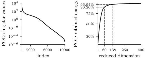
Figure 3: POD singular values (left) and corresponding retained energy (right) for the centered and scaled snapshot data.

In the following, we construct OpInf ROMs using reduced dimensions $r=60$ and $r=138$. The resulting ROM solutions are assessed using the strategies discussed in Section 3.3.

4.2 Predictions beyond the training time horizon

In the first set of experiments, we construct OpInf ROMs using the setup presented in Section 4.1 and employ them for predictions up to $t_{\mathrm{final}}=1\,000$. Prior to presenting our results for $\Gamma_{n}$ and $\Gamma_{c}$, we first do a qualitative assessment of the full field approximate solutions, which will be indicative of whether the OpInf ROMs issue predictions that resemble the complex turbulent structures of the reference fields.

Figure 4 plots the density field at four time instants: two within the training horizon ($t=525$ and $t=700$) and two within the prediction horizon ($t=800$ and $t=1\,000$).

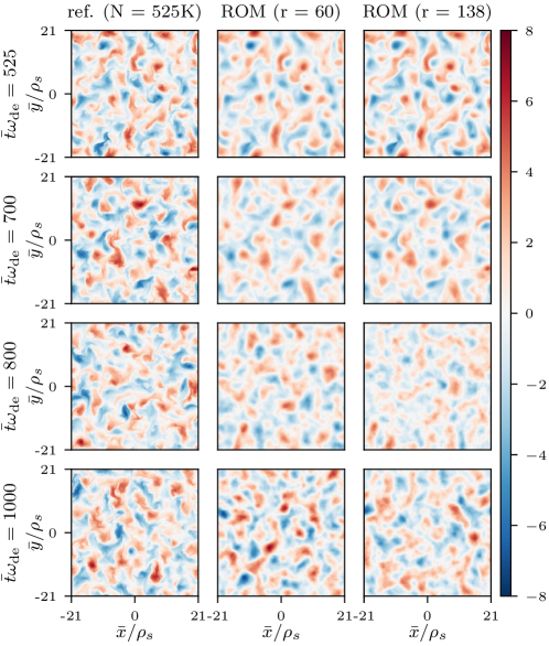
Figure 4: Predictions beyond the training time horizon: density field at four time instants. The first two ($t=525$ and $t=700$) fall within the training horizon, whereas the last two ($t=800$ and $t=1\;000$) are within the prediction time horizon.

Both ROMs provide accurate approximations of the large structures in the density field at the two time instants within the training horizon. The ROM with the larger reduced dimension, i.e., constructed using a POD basis that retains more energy, approximates well some of the smaller scale structures too. In the prediction horizon, the ROMs are not expected to accurately predict the complex and chaotic density field point-wisely. Indeed, the predictions do not match the reference data but they qualitatively resemble turbulent structures, where again the predictions corresponding to the ROM with $r=138$ are characterized by smaller scales structures as well. These results are encouraging and indicate that OpInf ROM could provide statistically accurate predictions for QoIs derived from the full fields such as $\Gamma_{n}$ and $\Gamma_{c}$.

We now shift our attention to the results for the two QoIs. We first plot the ROM approximations as well as the corresponding reference results obtained via DNS in Figure 5 for a qualitative assessment of the trends in the respective time traces.

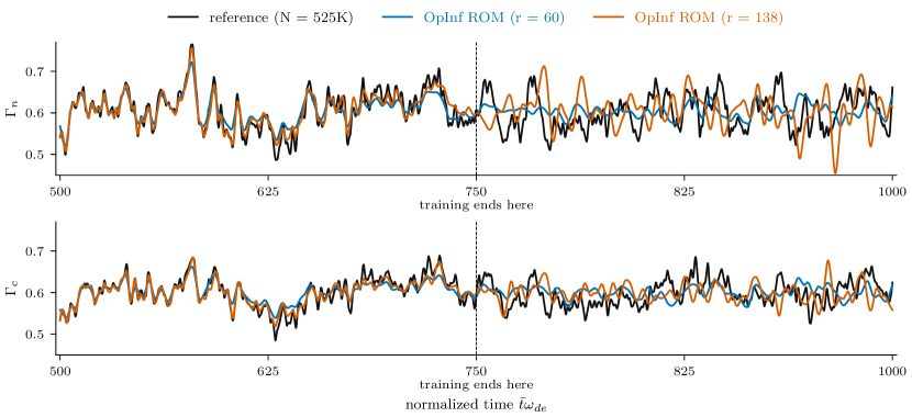
Figure 5: Predictions beyond the training time horizon: $\Gamma_{n}$ and $\Gamma_{c}$.

Both ROMs approximate the reference data accurately over the training horizon. However, the dynamics over the prediction horizon are damped for the OpInf ROM with $r=60$, whereas those corresponding to the larger OpInf ROM are richer and resemble the reference trends more accurately from a qualitative perspective.

We next assess the two OpInf ROM approximations statistically. The means and standard deviations are respectively shown in Tables 1 and 2.

Table 1: Predictions beyond the training time horizon: $\Gamma_{n}$ and $\Gamma_{c}$ statistics for the OpInf ROM with reduced dimension $r=60$.

interval	QoI	reference ($N=525$K)		OpInf ROM ($r=60$)
		mean	std. dev.	mean	std. dev.
training	$\Gamma_{n}$	0.6066	0.0467	0.6069	0.0308
	$\Gamma_{c}$	0.6018	0.0364	0.6018	0.0230
prediction	$\Gamma_{n}$	0.6012	0.0412	0.6037	0.0158
	$\Gamma_{c}$	0.5978	0.0296	0.6005	0.0143

Table 2: Predictions beyond the training time horizon: $\Gamma_{n}$ and $\Gamma_{c}$ statistics for the OpInf ROM with reduced dimension $r=138$.

interval	QoI	reference ($N=525$K)		OpInf ROM ($r=138$)
		mean	std. dev.	mean	std. dev.
training	$\Gamma_{n}$	0.6066	0.0467	0.6077	0.0395
	$\Gamma_{c}$	0.6018	0.0364	0.6007	0.0297
prediction	$\Gamma_{n}$	0.6012	0.0412	0.6044	0.0400
	$\Gamma_{c}$	0.5978	0.0296	0.5984	0.0215

Both ROMs accurately predict the QoI means over both training and prediction horizons. Moreover, they also accurately match the reference standard deviations over the training horizon. However, over the prediction horizon the smaller ROM underpredicts the turbulent fluctuations, the corresponding standard deviations are smaller than the reference results. In contrast, the larger ROM accurately approximates the standard deviations for both QoIs. Overall, the OpInf ROM with reduced dimension $r=138$ performs well and yields statistically accurate predictions for both QoIs.

For a more comprehensive assessment of our results, we next compute the respective power spectra and plot them in Figure 6. Both ROMs accurately capture the low-frequency part of the spectra for both training and prediction horizons. Furthermore, the ROM with reduced dimension $r=138$ accurately captures intermediate normalized frequencies up to $\sim 10^{-1}$ as well. However, both ROMs fail to capture the higher frequency content, where the small scale fluctuations dominate the dynamics, which is mainly due to the truncation of the linear POD basis used to compute these ROMs. This can be alleviated, for example, by introducing a closure model into the ROM [1, 16] or by constructing ROMs via non-linear methods [12]. Such an approach is beyond the scope of the present paper and will be considered in our future research.

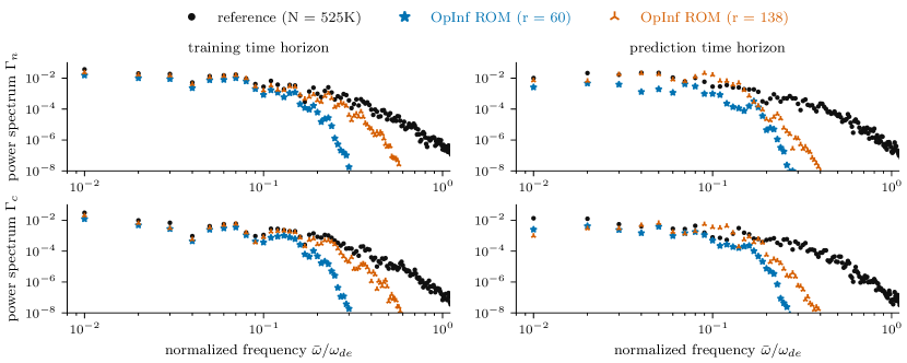
Figure 6: Predictions beyond the training time horizon: power spectra for $\Gamma_{n}$ and $\Gamma_{c}$.

Lastly, we report the runtimes for the two OpInf ROMs, averaged over $100$ runs. For the reduced dimension $r=60$, this is $3.8844\pm 0.1112$ seconds, which reduces the total runtime of the full high-fidelity simulation by nearly five orders of magnitude in single-core performance. The runtime of the ROM with larger reduced dimension is $13.8234\pm 0.6568$ seconds, i.e., a reduction of four orders of magnitude. The significant runtime reduction coupled with the statistical accuracy of the ROM solutions show that OpInf can be effectively used to construct statistically accurate ROMs for predictions beyond the training horizon, which amounts to a milestone towards real-time plasma turbulence simulations.

4.3 Predictions for other initial conditions

In the second set of experiments, we train ROMs using the same training data set as in the previous experiment but use them for predictions for other initial conditions. The predictions are made over the training horizon $[500,750)$, for which we have data corresponding to six other initial conditions.

While in principle we could reuse the OpInf ROMs from the previous experiment, the regularization hyperparameters in that context were tuned for predictions beyond the training time horizon. This, in turn, makes these ROMs less effective for predictions over the training time horizon for other initial conditions. We therefore retrain the OpInf ROMs, keeping in mind that this step is computationally cheap (see Section 3.2). We note that this experiment is more challenging than the previous one, in which OpInf ROMs were trained for predictions beyond the training time horizon. This is because here the reduced operators (and the corresponding regularization hyperparameters) are learned for a single data set but the resulting ROM is used for predictions for other initial conditions without having any other information about the corresponding dynamics. Therefore, obtaining accurate predictions in this context will indicate that OpInf can learn robust reduced plasma turbulence models.

Figure 7 plots the OpInf ROM predictions for $\Gamma_{n}$ for the six new initial conditions (labeled new IC $\#i$ for $i=1,2,\ldots,6$) and compares them with the high-fidelity reference data.

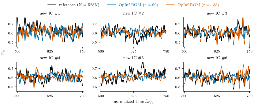
Figure 7: Predictions for other initial conditions: results for $\Gamma_{n}$.

Table 3: Predictions for other initial conditions: $\Gamma_{n}$ statistics for the OpInf ROM with reduced dimension $r=60$.

IC index	reference ($N=525$K)		OpInf ROM ($r=60$)
	mean	std. dev.	mean	std. dev.
1	0.6354	0.0468	0.6091	0.0423
2	0.6018	0.0470	0.6077	0.0298
3	0.6102	0.0432	0.6109	0.0260
4	0.6097	0.0429	0.6082	0.0325
5	0.6254	0.0515	0.6110	0.0185
6	0.6029	0.0405	0.6051	0.0238

Table 4: Predictions for other initial conditions: $\Gamma_{n}$ statistics for the OpInf ROM with reduced dimension $r=138$.

IC index	reference ($N=525$K)		OpInf ROM ($r=138$)
	mean	std. dev.	mean	std. dev.
1	0.6354	0.0468	0.6126	0.0375
2	0.6018	0.0470	0.6117	0.0270
3	0.6102	0.0432	0.6102	0.0489
4	0.6097	0.0429	0.6087	0.0331
5	0.6254	0.0515	0.6063	0.0213
6	0.6029	0.0405	0.6089	0.0436

As expected, the ROM predictions differ point-wisely from the reference chaotic solutions. However, the predictions (and especially those corresponding to $r=138$) capture the overall trends well. Furthermore, as shown in Tables 3 and 4, both ROMs provide accurate approximations for the respective means. The respective standard deviations are more accurately matched by the OpInf ROM with reduced dimension $r=138$. Note that the $\Gamma_{n}$ time trace corresponding new IC $\#5$ (bottom center plot in Figure 7) is topologically different from the time trace corresponding to the training data (cf. Figure 5). As a consequence, the standard deviation is less accurately approximated than for the other five initial conditions. Analogous results are obtained for $\Gamma_{c}$, as plotted in Figure 8 and shown in Tables 5 and 6.

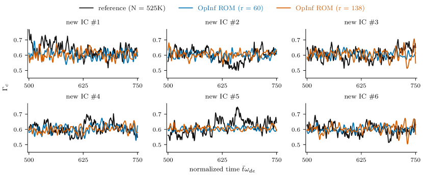
Figure 8: Predictions for other initial conditions: results for $\Gamma_{c}$.

Table 5: Predictions for other initial conditions: $\Gamma_{c}$ statistics for the OpInf ROM with reduced dimension $r=60$.

IC index	reference ($N=525$K)		OpInf ROM ($r=60$)
	mean	std. dev.	mean	std. dev.
1	0.6326	0.0411	0.6032	0.0258
2	0.5963	0.0394	0.6021	0.0200
3	0.6053	0.0369	0.6061	0.0183
4	0.6068	0.0356	0.6032	0.0246
5	0.6191	0.0463	0.6031	0.0114
6	0.5982	0.0321	0.5999	0.0153

Table 6: Predictions for other initial conditions: $\Gamma_{c}$ statistics for the OpInf ROM with reduced dimension $r=138$.

IC index	reference ($N=525$K)		OpInf ROM ($r=138$)
	mean	std. dev.	mean	std. dev.
1	0.6326	0.0411	0.6052	0.0264
2	0.5963	0.0394	0.6064	0.0213
3	0.6053	0.0369	0.6054	0.0309
4	0.6068	0.0356	0.6014	0.0206
5	0.6191	0.0463	0.6058	0.0128
6	0.5982	0.0321	0.6034	0.0274

We next compute the power spectra of the OpInf predictions corresponding to two initial conditions: one for which the predictions are accurate, new IC $\#$1, and the other for which they are less accurate, new IC $\#$5. We plot our results in Figure 9. For new IC $\#1$, both OpInf ROMs accurately capture the low and intermediate frequency range of the spectrum. Moreover, the ROM with larger reduced dimension captures part of the higher-frequency content as well. In contrast, for new IC $\#5$, for which the topology of the $\Gamma_{n}$ time trace is differs significantly from the training data, the ROM predictions fail to capture both low and high frequencies in the reference solutions.

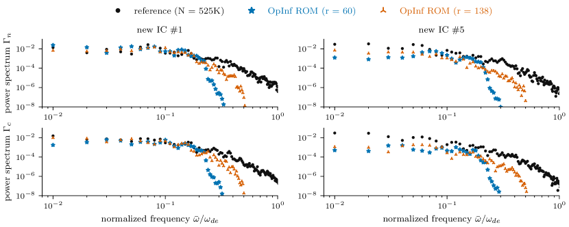
Figure 9: Predictions for other initial conditions: power spectra for $\Gamma_{n}$ and $\Gamma_{c}$ for two different initial conditions.

Lastly, the runtimes of the two ROMs, averaged over $100$ runs, are $1.9733\pm 0.0151$ seconds and $5.7724\pm 0.5992$ seconds, which reduce the total runtime of the full high-fidelity simulation by five and four orders of magnitude in single-core performance, respectively. Overall, these results show that OpInf ROMs constructed using DNS data corresponding to a single initial condition can provide computationally cheap and robust predictions for new initial conditions.

5 Summary and conclusions

Constructing accurate reduced-order models of nonlinear and chaotic plasma turbulence simulations is a very non-trivial task. However, when the goal is to obtain computationally cheap and statistically accurate approximations of key quantities of interest, this task can be accomplished by non-intrusive scientific machine learning reduced-order models. In the present paper, we proposed using Operator Inference for constructing such approximations. The only requirements for using Operator Inference are knowledge about the structure of the underlying governing equations and data to train a structure-preserving reduced model, which makes this approach flexible and easy to use in practice. As a representative example of a plasma turbulence model, we considered the Hasegawa-Wakatani equations that model two-dimensional electrostatic drift-wave turbulence and focused on two key quantities of interest: the particle flux and resistive dissipation rate. In a scenario characterized by complex dynamics, our results showed that Operator Inference can provide statistically accurate and robust approximations of the two quantities of interest, both beyond the training time horizon as well as for different initial conditions, while reducing the total runtime of the high-fidelity simulations by up to five orders of magnitude. In the broader context of fusion research, constructing such reduced models can have a substantial impact and amount to a milestone towards real-time plasma turbulence simulations as well as the design and control of optimized fusion devices.

Data availability statement

The high-fidelity simulation data were generated using the hw2d code [15]. The code and data to reproduce the results of this paper are available at https://gitlab.mpcdf.mpg.de/cgahr/learning-roms-for-hw.

References

- [1] S. E. Ahmed, S. Pawar, O. San, A. Rasheed, T. Iliescu, and B. R. Noack. On closures for reduced order models—A spectrum of first-principle to machine-learned avenues. Physics of Fluids, 33(9):091301, 2021.
- [2] A. Arakawa. Computational Design for Long-Term Numerical Integration of the Equations of Fluid Motion: Two-Dimensional Incompressible Flow. Part I. Journal of computational physics, 135(2):103–114, 1997.
- [3] P. Benner, S. Gugercin, and K. Willcox. A Survey of Projection-Based Model Reduction Methods for Parametric Dynamical Systems. SIAM Review, 57(4):483–531, 2015.
- [4] G. Berkooz, P. Holmes, and J. L. Lumley. The Proper Orthogonal Decomposition in the Analysis of Turbulent Flows. Annual Review of Fluid Mechanics, 25(1):539–575, 1993.
- [5] S. J. Camargo, D. Biskamp, and B. D. Scott. Resistive drift-wave turbulence. Physics of Plasmas, 2(1):48–62, Jan. 1995.
- [6] J. L. de Sousa Almeida, A. C. Pires, K. F. V. Cid, and A. C. N. Junior. Non-Intrusive Reduced Models based on Operator Inference for Chaotic Systems. 2022.
- [7] F. Faraji, M. Reza, A. Knoll, and J. N. Kutz. Dynamic mode decomposition for data-driven analysis and reduced-order modeling of E × B plasmas: I. Extraction of spatiotemporally coherent patterns. Journal of Physics D: Applied Physics, 57(6):065201, Nov. 2023.
- [8] F. Faraji, M. Reza, A. Knoll, and J. N. Kutz. Dynamic mode decomposition for data-driven analysis and reduced-order modeling of E × B plasmas: II. Dynamics forecasting. Journal of Physics D: Applied Physics, 57(6):065202, Nov. 2023.
- [9] I. Farcas, R. Gundevia, R. Munipalli, and K. E. Willcox. Parametric non-intrusive reduced-order models via operator inference for large-scale rotating detonation engine simulations. In AIAA SCITECH 2023 Forum. American Institute of Aeronautics and Astronautics, Jan. 2023.
- [10] I. Farcas, R. Munipalli, and K. E. Willcox. On filtering in non-intrusive data-driven reduced-order modeling. In AIAA AVIATION 2022 Forum, AIAA AVIATION Forum. American Institute of Aeronautics and Astronautics, June 2022.
- [11] S. Futatani, S. Benkadda, and D. del-Castillo-Negrete. Spatiotemporal multiscaling analysis of impurity transport in plasma turbulence using proper orthogonal decomposition. Physics of Plasmas, 16(4):042506, Apr. 2009.
- [12] R. Geelen, S. Wright, and K. Willcox. Operator inference for non-intrusive model reduction with quadratic manifolds. Computer Methods in Applied Mechanics and Engineering, 403:115717, Jan. 2023.
- [13] G. H. Golub and C. F. V. Loan. Matrix Computations. The Johns Hopkins University Press, 2013.
- [14] I. R. Goumiri, C. W. Rowley, Z. Ma, D. A. Gates, J. A. Krommes, and J. B. Parker. Reduced-order model based feedback control of the Modified Hasegawa-Wakatani model. Physics of Plasmas, 20(4):042501, Apr. 2013.
- [15] R. Greif. HW2D: A reference implementation of the Hasegawa-Wakatani model for plasma turbulence in fusion reactors. Journal of Open Source Software, 8(92):5959, Dec. 2023.
- [16] R. Greif, F. Jenko, and N. Thuerey. Physics-Preserving AI-Accelerated Simulations of Plasma Turbulence, Sept. 2023.
- [17] A. Hasegawa and K. Mima. Pseudo-three-dimensional turbulence in magnetized nonuniform plasma. Physics of Fluids, 21(1):87–92, Jan. 1978.
- [18] A. Hasegawa and M. Wakatani. Plasma Edge Turbulence. Physical Review Letters, 50(9):682–686, Feb. 1983.
- [19] R. A. Heinonen and P. H. Diamond. Turbulence model reduction by deep learning. Physical Review E, 101(6):061201, June 2020.
- [20] O. Issan and B. Kramer. Predicting Solar Wind Streams from the Inner-Heliosphere to Earth via Shifted Operator Inference. Journal of Computational Physics, 473:111689, Jan. 2023.
- [21] Y. Jajima, M. Sasaki, R. T. Ishikawa, M. Nakata, T. Kobayashi, Y. Kawachi, and H. Arakawa. Estimation of 2D profile dynamics of electrostatic potential fluctuations using multi-scale deep learning. Plasma Physics and Controlled Fusion, 65(12):125003, Oct. 2023.
- [22] A. A. Kaptanoglu, K. D. Morgan, C. J. Hansen, and S. L. Brunton. Characterizing magnetized plasmas with dynamic mode decomposition. Physics of Plasmas, 27(3):032108, Mar. 2020.
- [23] P. Khodabakhshi and K. E. Willcox. Non-intrusive data-driven model reduction for differential–algebraic equations derived from lifting transformations. Computer Methods in Applied Mechanics and Engineering, 389:114296, Feb. 2022.
- [24] B. Kramer and K. E. Willcox. Nonlinear Model Order Reduction via Lifting Transformations and Proper Orthogonal Decomposition. AIAA Journal, 57(6):2297–2307, June 2019.
- [25] A. Kusaba, T. Kuboyama, and S. Inagaki. Sparsity-Promoting Dynamic Mode Decomposition of Plasma Turbulence. Plasma and Fusion Research, 15:1301001–1301001, 2020.
- [26] P. Manz. The Microscopic Picture of Plasma Edge Turbulence. habilitation, Technische Universität München, 2019.
- [27] S. A. McQuarrie, C. Huang, and K. E. Willcox. Data-driven reduced-order models via regularised Operator Inference for a single-injector combustion process. Journal of the Royal Society of New Zealand, 51(2):194–211, Apr. 2021.
- [28] R. Numata, R. Ball, and R. L. Dewar. Bifurcation in electrostatic resistive drift wave turbulence. Physics of Plasmas, 14(10):102312, Oct. 2007.
- [29] B. Peherstorfer and K. Willcox. Data-driven operator inference for nonintrusive projection-based model reduction. Computer Methods in Applied Mechanics and Engineering, 306:196–215, July 2016.
- [30] E. Qian, I.-G. Farcas, and K. Willcox. Reduced operator inference for nonlinear partial differential equations. SIAM Journal on Scientific Computing, 44(4):A1934–A1959, 2022.
- [31] E. Qian, B. Kramer, B. Peherstorfer, and K. Willcox. Lift & Learn: Physics-informed machine learning for large-scale nonlinear dynamical systems. Physica D: Nonlinear Phenomena, 406:132401, May 2020.
- [32] C. Runge. Ueber die numerische Auflösung von Differentialgleichungen. Mathematische Annalen, 46(2):167–178, June 1895.
- [33] M. Sasaki, T. Kobayashi, R. O. Dendy, Y. Kawachi, H. Arakawa, and S. Inagaki. Evaluation of abrupt energy transfer among turbulent plasma structures using singular value decomposition. Plasma Physics and Controlled Fusion, 63(2):025004, Dec. 2020.
- [34] R. Swischuk, B. Kramer, C. Huang, and K. Willcox. Learning physics-based reduced-order models for a single-injector combustion process. AIAA Journal, 58(6):2658–2672, June 2020.
- [35] R. Taylor, J. N. Kutz, K. Morgan, and B. Nelson. Dynamic Mode Decomposition for Plasma Diagnostics and Validation. Review of Scientific Instruments, 89(5):053501, May 2018.
- [36] W. I. T. Uy, D. Hartmann, and B. Peherstorfer. Operator inference with roll outs for learning reduced models from scarce and low-quality data. Computers & Mathematics with Applications, 145:224–239, Sept. 2023.
- [37] M. Wakatani and A. Hasegawa. A collisional drift wave description of plasma edge turbulence. The Physics of Fluids, 27(3):611–618, Mar. 1984.
- [38] P. Welch. The Use of Fast Fourier Transform for the Estimation of Power Spectra: A Method Based on Time Averaging Over Short, Modified Periodograms. IEEE Transactions on Audio and Electroacoustics, 15(2):70–73, June 1967.
- [39] G. Yatomi, M. Nakata, and M. Sasaki. Data-driven modal analysis of nonlinear quantities in turbulent plasmas using multi-field singular value decomposition. Plasma Physics and Controlled Fusion, 65(9):095014, Sept. 2023.