DiffDA: a diffusion model for weather-scale data assimilation

Abstract

The generation of initial conditions via accurate data assimilation is crucial for reliable weather forecasting and climate modeling. We propose the DiffDA as a machine learning based data assimilation method capable of assimilating atmospheric variables using predicted states and sparse observations. We adapt the pretrained GraphCast weather forecast model as a denoising diffusion model.

Our method applies two-phase conditioning: on the predicted state during both training and inference, and on sparse observations during inference only. As a byproduct, this strategy also enables the post-processing of predictions into the future, for which no observations are available.

Through experiments based on a reanalysis dataset, we have verified that our method can produce assimilated global atmospheric data consistent with observations at 0.25degree resolution. The experiments also show that the initial conditions that are generated via our approach can be used for forecast models with a loss of lead time of at most 24 hours when compared to initial conditions of state-of-the-art data assimilation suites. This enables to apply the method to real world applications such as the creation of reanalysis datasets with autoregressive data assimilation.

1 Introduction

Modern weather forecasts rely heavily on numerical weather predictions. The quality of these predictions depends on the data assimilation process that is used to generate initial conditions on the model grid, based on sparse observations available at different locations. Errors in initial conditions are one of the main sources for errors in weather forecasts [Bonavita et al., 2016]. Additionally, data assimilation is employed in creating reanalysis datasets, such as the ERA5 dataset, which contains reconstructed historical weather variables as grided fields [Hersbach et al., 2020]. Reanalysis datasets play a central role in weather and climate research [ipc, 2023], and are essential for the training of global, machine learned weather forecast models [Pathak et al., 2022, Bi et al., 2023, Lam et al., 2023].

Various data assimilation methods have been developed and employed to address different characteristics of observation data and system dynamics. Among those, variational data assimilation and ensemble Kalman filter are the two most applied families of methods in operational data assimilation [Bannister, 2017]. The variational method is solving an optimization problem minimizing a cost function which measures the discrepancy between forecast simulations of the previous prediction and the real observations. It requires multiple iterations in which linearized observations and evolution functions are evaluated to compute the gradient of the cost function. The linearized observation and evolution function have to be implemented separately. This adds extra overheads because the linearized functions have similar complexity as the original function, and a lot of efforts have to be invested to maintain the consistency of the original code and the linearized code. The ensemble Kalman filter method updates the state estimation according to the covariance matrix calculated from ensemble simulations. Both approaches are computation intensive as one requires multiple optimization iterations and the other requires multiple ensemble simulations.

Data assimilation tools are becoming a bottleneck in the simulation pipeline. While traditional data assimilation methods are sufficiently competent in operational weather forecasts [Bonavita et al., 2016], their high costs restrict broader adoptions, making them tightly coupled with a specific numerical weather forecast model. This restriction becomes more evident since the explosion of ML weather forecast models [Pathak et al., 2022, Lam et al., 2023, Bi et al., 2023]. Those models claim to be a replacement of the traditional models by achieving competitive or even superior accuracy compared to the best operational model while being orders of magnitude faster. Ironically, they cannot independently make forecasts as they are all trained and evaluated on the ERA5 dataset [Hersbach et al., 2020] which is produced by the traditional data assimilation method together with the numerical forecast model. In fact, data assimilation is the last major obstacle to achieve a pure ML weather forecast pipeline.

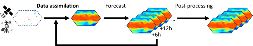
Figure 1: Diagram of numerical weather forecast pipeline. It consists of data assimilation, forecast and post-processing. Data assimilation produces gridded values from sparse observations and predicted gridded values from previous time steps. Forecast takes in gridded values and produces predictions in gridded values at future time steps. Post-processing improves forecast results such that it is closer to future observations.

In a probabilistic view, data assimilation can be formulated as sampling from a probability distribution of atmosphere states conditioned on observations and predicted states [Law et al., 2015, Evensen et al., 2022]. Capable of solving the conditional sampling problem, denoising diffusion models [Ho et al., 2020] naturally become a tentative choice for data assimilation. Moreover, the blooming community of diffusion models provides an arsenal of techniques for enforcing conditions of different kinds. In particular, conditioning techniques for in-painting [Lugmayr et al., 2022, Song et al., 2020] and super-resolution [Saharia et al., 2022, Chung et al., 2022] are of special interest, because they are similar to conditioning of observations and predicted states respectively. This denoising diffusion model approach has been applied in relatively small scale data assimilation problems [Rozet and Louppe, 2023a, b, Finn et al., 2023, Andry et al., 2023], but none of them is able to assimilate data with a resolution comparable with the ERA5 dataset (0.25 degree horizontal resolution) thus limiting their use with ML forecast models. Similarly, the denoising diffusion techniques have been applied in weather forecasts [Andrychowicz et al., 2023] and post-processing [Mardani et al., 2023, 2024, Li et al., 2023]. In particular, Price et al. developed the GenCast which is capable of doing ensemble forecast at 1 degree resolution.

In this work, we propose a new approach of data assimilation based on the denoising diffusion model with a focus on weather and climate applications. We are able to scale to 0.25degree resolution with 13 vertical levels by utilizing an established ML forecast model GraphCast [Lam et al., 2023] as the backbone of the diffusion model. As we do not have real-world observations available from the ERA5 dataset, we are using grid columns of the ERA5 reanalysis dataset as proxies for observations. During training, the diffusion model is conditioned with background of previous predictions – meaning the state produced by the forecast model using states of forecasts from earlier initial conditions. During inference, we further condition the model with sparse column observations following Repaint [Lugmayr et al., 2022]. In addition, we use a soft mask and interpolated observations to strengthen the conditioning utilizing the continuity of atmosphere variables. The resulting assimilated data can indeed converge to the ground truth data when increasing the number of sampled columns. More importantly, it is able to be used as the inputs of the forecast model where its 48h forecast error also converge to the 48h forecast error with ground truth inputs. We also test the autoregressive data assimilation to generate reanalysis dataset given a time series of observations and an initial predicted field which turns out to be consistent with the ERA5 dataset.

Our key contributions are:

1. We demonstrate a novel machine learning (ML) based data assimilation method capable of assimilating high resolution data. The assimilated data is ready for weather forecast applications.

2. We are able to create data assimilation cycles combining our method and a machine learning forecast model. The resulting reanalysis dataset is consistent with the ERA5 dataset.

3. We build our method using a neural network backbone from a trained machine learning based forecast model. It is easy to upgrade the backbone with any state-of-the-art model due to the flexibility of our method.

4. Our method opens up the possibility of a pure machine learning weather forecast pipeline consisting of data assimilation, forecasting, and post-processing.

2 Method

2.1 Problem formulation

The goal of data assimilation is to reconstruct atmospheric variables on a given grid with $n$ grid points $\mathbf{x}_{i}\in\mathbb{R}^{n}$ at physical time step $i$ given $m$ measurements $\mathbf{y}_{i}=f(\mathbf{x}^{*}_{i}),\mathbf{y}_{i}\in\mathbb{R}^{m},\mathbf{x}_{i}^{*}\in\mathbb{R}^{n}$ where $\mathbf{x}^{*}_{i}$ is the ground truth of atmospheric variables on grid points at time step $i$. In addition, estimated values on grid points $\hat{\mathbf{x}}_{i}=\mathcal{F}(\mathbf{x}_{i-1})$ produced by the forecast model $\mathcal{F}:\mathbb{R}^{n}\rightarrow\mathbb{R}^{n}$ are also provided as the inputs. In a probabilistic view, data assimilation samples from a conditional distribution $p(\mathbf{x}_{i}|\hat{\mathbf{x}}_{i},\mathbf{y}_{i})$ which minimizes the discrepancy between $\mathbf{x}_{i}$ and $\mathbf{x}^{*}_{i}$. To simplify the problem, $f$ is limited to a sparse linear observation operator $\mathbf{y}_{i}=f(\mathbf{x}^{*})=\mathbf{Ax}^{*}$ where $\mathbf{A}$ is a sparse matrix with only one nonzero value in each row. In real world cases, this simplification applies to point observations such as temperature, pressure, and wind speed measurements at weather stations and balloons.

2.2 Denoising diffusion probabilistic model

The denoising diffusion probabilistic model (DDPM) is a generative model capable of sampling from the probabilistic distribution defined by the training data [Ho et al., 2020]. It is trained to approximate the reverse of the diffusion process where noise is added to a state vector $\mathbf{x}^{0}$ during $N$ diffusion steps resulting in an isotropic Gaussian noise vector $\mathbf{x}^{N}\sim\mathcal{N}(\mathbf{0},\mathbf{I})$. We denote the state vector at physical time step $i$ and diffusion step $j$ with $\mathbf{x}^{j}_{i}$. We write $\mathbf{x}^{j}$ whenever the statement is independent of the physical time step. Note that the diffusion step $j$ and the physical time step $i$ are completely independent of each other.

For each diffusion step $j$, the diffusion process can be seen as sampling from a Gaussian distribution with a mean of $\sqrt{1-\beta_{j}}\mathbf{x}^{j-1}$ and covariance matrix of $\beta_{j}\mathbf{I}$:

$$p(\mathbf{x}^{j}|\mathbf{x}^{j-1})=\mathcal{N}(\sqrt{1-\beta_{j}}\mathbf{x}^{j-1},\beta_{j}\mathbf{I})$$ (1)

where $\beta_{j}>0$ is the variance schedule.

A denoising diffusion model $\mathbf{\mu}_{\theta}$ is used to predict the mean of $\mathbf{x}^{j-1}$ given $\mathbf{x}^{j}$ and $j$ with the following parameterization:

$$\mu_{\theta}(\mathbf{x}^{j},j)=\frac{1}{\sqrt{1-\beta_{j}}}\left(\mathbf{x}^{j}-\frac{\beta_{j}}{\sqrt{1-\bar{\alpha}_{j}}}\epsilon_{\theta}(\mathbf{x}^{j},j)\right)$$ (2)

where $\theta$ are the trainable parameters, $\bar{\alpha}_{j}=\prod_{s=1}^{j}{(1-\beta_{s})}$. Then, $\mathbf{x}^{j-1}$ can be sampled from $p(\mathbf{x}^{j-1}|\mathbf{x}^{j})=\mathcal{N}(\mu_{\theta}(\mathbf{x}^{j},j),\frac{1-\bar{\alpha}_{j-1}}{1-\bar{\alpha}_{j}}\beta_{t}\mathbf{I})$ to reverse the diffusion process. Applying this procedure $N$ times from $\mathbf{x}^{N}\sim\mathcal{N}(\mathbf{0},\mathbf{I})$, we can generate $\mathbf{x}^{0}$ which follows a similar distribution as the empirical distribution of the training data.

During the training phase, we minimize the following loss function:

$$L(\theta)=\mathbb{E}_{j\sim U[1,N],\mathbf{x}^{0*}\sim\text{training data},\epsilon\sim\mathcal{N}(\mathbf{0},\mathbf{I})}\left[\|\epsilon-\epsilon_{\theta}(\mathbf{x}^{j},j)\|^{2}\right].$$ (3)

$\mathbf{x}^{j}$ can be expressed in a closed form: $\mathbf{x}^{j}=\sqrt{\bar{\alpha}_{j}}\mathbf{x}^{0*}+\sqrt{(1-\bar{\alpha}_{j})}\epsilon$ because the diffusion process applies independent Gaussian noise at each step, and thus $p(\mathbf{x}^{j}|\mathbf{x}^{0*})=\mathcal{N}(\sqrt{\bar{\alpha}_{j}}\mathbf{x}^{0*},(1-\bar{\alpha}_{j})\mathbf{I})$.

With the unconditional denoising diffusion model above, we add the conditioning of predicted state $\hat{\mathbf{x}}$ and observation $\mathbf{y}$ separately according to their characteristics.

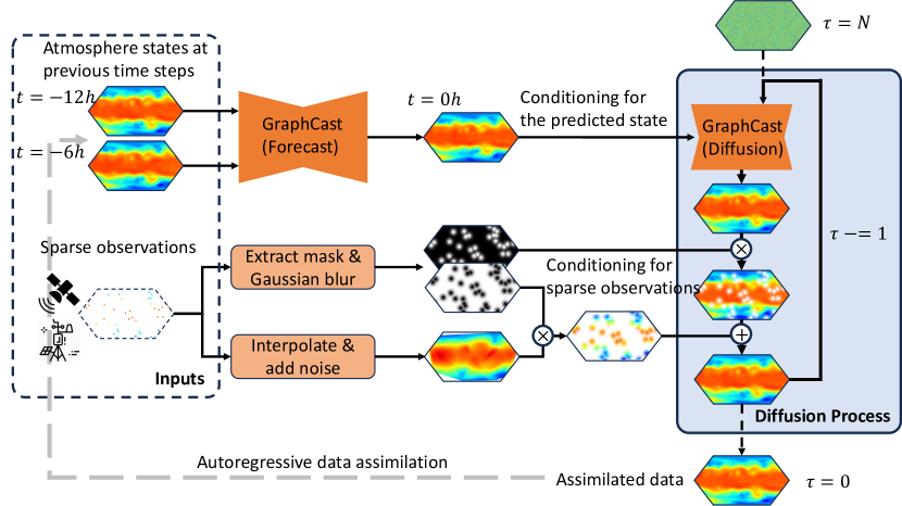
Figure 2: Architecture of the diffusion based data assimilation method. We take advantage of the input and output shape of the pretrained GraphCast model which takes the state of the atmosphere at two time steps as input. In each iteration of the denoising diffusion process in our method, the adapted GraphCast model takes the predicted state and the assimilated state with noise, and further denoises assimilated state. To enforce the observations at inference time, the denoised state is merged with interpolated observations using a soft mask created by blurring the hard mask of the original observations.

2.3 Conditioning for predicted state

Utilizing the fact that the predicted state $\hat{\mathbf{x}}$ has the same shape as the diffused state $\mathbf{x}^{j}$, it is convenient to add the predicted state as an additional input for the (reparameterized) diffusion model denoted as $\epsilon_{\theta}(\mathbf{x}^{j},\hat{\mathbf{x}},j)$ [Saharia et al., 2022]. The underlying neural network can concatenate $\mathbf{x}^{j}$ and $\hat{\mathbf{x}}$ in their feature channels without changing its architecture as shown in Figure 2.

Since $\epsilon_{\theta}$ (and $\mu_{\theta}$) is dependent on $\hat{\mathbf{x}}$, the reverse diffusion process becomes sampling from $p(\mathbf{x}^{j-1}|\mathbf{x}^{j},\hat{\mathbf{x}})=\mathcal{N}(\mu_{\theta}(\mathbf{x}^{j},\hat{\mathbf{x}},j),\frac{1-\bar{\alpha}_{j-1}}{1-\bar{\alpha}_{j}}\beta_{j}\mathbf{I})$. Therefore, the generated $\mathbf{x}^{0}$ is sampled from the conditional distribution $p(\mathbf{x}^{0}|\hat{\mathbf{x}})=p(\mathbf{x}^{N})\prod_{j=1}^{N}{p(\mathbf{x}^{j-1}|\mathbf{x}^{j},\hat{\mathbf{x}})}$.

This method requires sampling pairs of $\mathbf{x}^{0*}$ and $\hat{\mathbf{x}}$ during training. This can be realized by sampling two states $\mathbf{x}_{i-1}^{*},\mathbf{x}_{i}^{*}$ with consecutive physical time steps from training data, and then apply the forecast model to get the predicted state at physical time $i$: $\hat{\mathbf{x}}_{i}=\mathcal{F}(\mathbf{x}_{i-1}^{*})$. Afterwards, the sampled (ground truth) state $\mathbf{x}_{i}^{*}$ is diffused with random $j\in[1,N]$ steps which is implemented with the closed form formula: $\mathbf{x}^{j}_{i}=\sqrt{\bar{\alpha}_{j}}\mathbf{x}^{0*}_{i}+\sqrt{(1-\bar{\alpha}_{j})}\epsilon,\epsilon\sim\mathcal{N}(\mathbf{0},\mathbf{I})$. Finally, we can take one gradient step based on $\nabla_{\theta}\|\epsilon-\epsilon_{\theta}(\mathbf{x}^{j}_{i},\hat{\mathbf{x}}_{i},j)\|^{2}$ to train the diffusion model.

With the conditioning of the predicted state alone, we can already perform backward diffusion steps using the trained model $\mu_{\theta}$ which results in $\mathbf{x}^{0}\sim p(\mathbf{x}^{0}|\hat{\mathbf{x}})$. This means we corrected, or in other words, “post-processed” the forecast result $\hat{\mathbf{x}}$ to be closer to the ground truth state $\mathbf{x}^{*}$.

2.4 Conditioning for sparse observations

The conditioning for sparse observations poses a different challenge than the conditioning on the predicted state. The sparse observations $\mathbf{y}$ have a variable length $m$ as opposed to a fixed length $n$, and the data assimilation results are invariant to the permutation of the $m$ elements in $\mathbf{y}$. This requires dedicated design in the neural network if we want to directly condition $\mu_{\theta}$ with $\mathbf{y}$ as before. Even if we find a solution to implement that, the trained diffusion model will have an generalization problem because the possible input space spanned by $\mathbf{x}^{0}$, $\hat{\mathbf{x}}$, and $\mathbf{y}$ is too large and hard to thoroughly sample during training.

To avoid those issues, we follow inpainting techniques [Lugmayr et al., 2022, Song et al., 2020] to enforce the conditioning of observations at inference time. Let us start with a simple approach first. It creates a hard mask $\mathbf{m}_{h}\in\{0,1\}^{n}$ to indicate which grid columns of the reanalysis state is observed, where a 1 means the associated value in $\mathbf{x}^{*}$ is observed in $\mathbf{y}$ and vice versa. The mask equals the sum of the columns of the observation matrix $\mathbf{A}\in\mathbb{R}^{n\times m}$ where $\mathbf{y}=\mathbf{Ax}^{*}$. During the inference of the diffusion model, a state vector with white Gaussian noise is created and gradually denoised by the denoising diffusion model. However, with $\mathbf{y}$ present, we have better knowledge over the observed locations in the state vector. For those locations, values can be produced by a forward diffusion process from the observation data. We can use the mask $\mathbf{m}_{h}$ to treat the two parts separately and combine them in each iteration of the denoising process (Figure 2).

$$\mathbf{x}^{j-1}_{\text{known}} \sim\mathcal{N}(\sqrt{\bar{\alpha}^{j-1}}\mathbf{x}^{*},(1-\bar{\alpha}^{j-1})\mathbf{I})$$

$$\mathbf{x}^{j-1}_{\text{unknown}} \sim\mathcal{N}(\mu_{\theta}(\mathbf{x}^{j},j),\frac{1-\bar{\alpha}_{j-1}}{1-\bar{\alpha}_{j}}\beta_{t}\mathbf{I})$$

$$\mathbf{x}^{j-1} =\mathbf{m}_{h}\odot\mathbf{x}^{j-1}_{\text{known}}+(1-\mathbf{m}_{h})\odot\mathbf{x}^{j-1}_{\text{unknown}}$$

Here, $\odot$ denotes point-wise multiplication used to filter observed and non-observed values. Although this method can guide diffusion result to the observed values, it performs poorly in practice because only the values at the observation locations are forced to the given values while other values remain unchanged as in the unconditional scenario. This is likely related to the encoding-process-decoding architecture commonly used in diffusion models: the encoding and decoding layers employ pooling to downscale and upscale in spatial dimensions. While it helps to condense information and reduce calculations, it also smears out local details. As a result, the added conditioning information is often lost during this process.

We tackle this issue by using a “soft mixing” instead of a hard one. In the soft mixing, we replace the hard mask $\mathbf{m}_{h}$ with a soft mask $\mathbf{m}_{s}$ by applying a Gaussian blur to $\mathbf{m}_{h}$ with standard deviation $\sigma_{G}$, diameter $d$ and re-normalize it to the range of [0, 1]. In this case, the support region of $\mathbf{m}_{s}$ (where its values are larger than 0) is larger than the support region of the observed values. As the atmosphere variables are relatively continuous over space, we interpolate the observed values to fill the support region of $\mathbf{m}_{s}$. While we interpolate all the atmospheric variables in the same way assuming they have similar continuity, it is also possible to adjust the area of support regions for each variable according to its continuity. Thus the inference iteration becomes:

$$\begin{split}\mathbf{m}^{\prime}_{s}&=\text{Gaussianblur}(\mathbf{m}_{h},\sigma_{G},d)\\ \mathbf{m}_{s}&=\mathbf{m}^{\prime}_{s}/\max{(\mathbf{m}^{\prime}_{s})}\\ {\mathbf{x}^{*}}^{\prime}&=\text{Interpolate}(\mathbf{m}_{h}\odot\mathbf{x}^{*},d)\\ \mathbf{x}^{j-1}_{\text{known}}&\sim\mathcal{N}(\sqrt{\bar{\alpha}^{j-1}}{\mathbf{x}^{*}}^{\prime},(1-\bar{\alpha}^{j-1})\mathbf{I})\\ \mathbf{x}^{j-1}_{\text{unknown}}&\sim\mathcal{N}(\mu_{\theta}(\mathbf{x}^{j},j),\frac{1-\bar{\alpha}_{j-1}}{1-\bar{\alpha}_{j}}\beta_{t}\mathbf{I})\\ \mathbf{x}^{j-1}&=\mathbf{m}_{s}\odot\mathbf{x}^{j-1}_{\text{known}}+(1-\mathbf{m}_{s})\odot\mathbf{x}^{j-1}_{\text{unknown}}.\end{split}$$ (4)

In addition, we also applied the resampling technique from [Lugmayr et al., 2022] to further reduce the inconsistency between the known part and unknown part. For each denoising iteration, the resampling technique repeats the iteration $U$ times by pulling the resulting $\mathbf{x}^{j-1}$ back to $\mathbf{x}^{j}$ with the forward diffusion process (missing) 1 and repeating the denoising step (missing) 4. The overall algorithm of applying denosing diffusion model for data assimilation is presented in Algorithm 1.

Algorithm 1 Data assimilation (inference)

0:  predicted state $\hat{\mathbf{x}}$, hard mask of observations $\mathbf{m}_{h}$, observation values at grid points $\mathbf{m}_{h}\odot\mathbf{x}^{*}$ (created from observation vector $\mathbf{y}$, and observation operator $\mathbf{A}$), covariance schedule $\beta_{j},j=1,\cdots,N$, Gaussian blur standard deviation $\sigma_{G}$, Gaussian blur diameter $d$, scaling factor $\mathbf{s}$

0:  $\mathbf{x}\sim p(\mathbf{x}|\hat{\mathbf{x}},\mathbf{y})$

  $\mathbf{m}^{\prime}_{s}=\text{Gaussianblur}(\mathbf{m}_{h},\sigma_{G},d)$

  $\mathbf{m}_{s}=\mathbf{m}^{\prime}_{s}/\max{(\mathbf{m}^{\prime}_{s})}$

  ${\mathbf{x}^{*}}^{\prime}=\text{Interpolate}(\mathbf{m}_{h}\odot\mathbf{x}^{*},d)$

  $\mathbf{x}^{N}\sim\mathcal{N}(\mathbf{0},\mathbf{I})$

  for j in $N,\cdots,1$ do

     Conditioning for predicted state

        $\bar{\alpha}_{j}=\prod_{s=1}^{j}{(1-\beta_{s})}$

        $\bar{\mathbf{x}}^{j-1}_{\text{unknown}}=\frac{1}{\sqrt{1-\beta_{j}}}\left(\mathbf{x}^{j}-\frac{\beta_{j}}{\sqrt{1-\bar{\alpha}_{j}}}\epsilon_{\theta}(\mathbf{x}^{j},\hat{\mathbf{x}},j)\right)$

        $\mathbf{x}^{j-1}_{\text{unknown}}\sim\mathcal{N}(\bar{\mathbf{x}}^{j-1}_{\text{unknown}},\frac{1-\bar{\alpha}_{j-1}}{1-\bar{\alpha}_{j}}\beta_{t}\mathbf{I})$

     Conditioning for sparse observations

        $\mathbf{x}^{j-1}_{\text{known}}\sim\mathcal{N}(\sqrt{\bar{\alpha}^{j-1}}{\mathbf{x}^{*}}^{\prime},(1-\bar{\alpha}^{j-1})\mathbf{I})$

        $\mathbf{x}^{j-1}=\mathbf{m}_{s}\odot\mathbf{x}^{j-1}_{\text{known}}+(1-\mathbf{m}_{s})\odot\mathbf{x}^{j-1}_{\text{unknown}}$

  end for

  $\mathbf{x}=\hat{\mathbf{x}}+\mathbf{s}\odot\mathbf{x}^{0}$ (apply skip connection)

2.5 Selection of diffusion model structure

Our method provides a lot of flexibility on the selection of the neural network structure for $\epsilon_{\theta}(\mathbf{x}^{j}_{i},\hat{\mathbf{x}}_{i},j):\mathbb{R}^{n}\times\mathbb{R}^{n}\times\mathbb{N}^{+}\rightarrow\mathbb{R}^{n}$ as any neural network that matches the function signature will work. However, $n$ can be a large number of tens of millions in practice rendering many neural network architectures infeasible due to resource constraints. It is crucial for a neural network to utilize the spatial information in the state vector $\mathbf{x}$ in order to learn efficiently.

Instead of creating a new architecture, we employ a proven architecture in ML weather forecast models which has a similar signature $\mathbb{R}^{c\cdot n}\rightarrow\mathbb{R}^{n},c\in\mathbb{N}^{+}$. Due to this similarity, neural networks that perform well in forecasting should also do well in data assimilation task, and it is likely to take less training steps using pretrained weights of the forecast model when training the diffusion model. Moreover, thanks to this, we can adapt the neural network structure with ease from any state-of-the-art weather forecast model.

3 Experiments

3.1 Implementation

We demonstrate our method in a real-world scenario with a horizontal resolution of 0.25 degree and 13 vertical levels. This matches the resolution of the WeatherBench2 dataset [Rasp et al., 2023] used by state-of-the-art ML weather forecast models. We take the GraphCast model as the backbone of the diffusion model because the pretrained model takes in states at two consecutive time steps $\mathbf{x}_{i-1},\mathbf{x}_{i}$ to predict $\mathbf{x}_{i+1}$ which takes much less effort than other forecast models to re-purpose it to $\epsilon_{\theta}(\mathbf{x}^{j}_{i},\hat{\mathbf{x}}_{i},j)$ given that there is one-to-one matching between $\mathbf{x}_{i-1}$ and $\mathbf{x}^{j}_{i}$, as well as $\mathbf{x}_{i+1}$ and $\hat{\mathbf{x}}_{i}$. As is determined by the pretrained GraphCast model, the input size $n$ is set to $(6\times 13+5)\times 721\times 1440$ where there are 6 pressure level variables, 5 surface level variables, 13 pressure levels, 721 latitude and 1440 longitude grid points on a longitude-latitude horizontal grid.

The diffusion model is implemented with the jax library [Bradbury et al., 2018] and the official implementation of GraphCast. We use the AdamW optimizer [Loshchilov and Hutter, 2018] with a warm-up cosine annealing learning rate schedule and data parallel training on 80 AMD MI250 GPUs with a (global) batch size of 80 for 12 epochs. Gradient checkpoints are added in the GraphCast model to reduce the GPU memory footprint.

3.2 Training data

We use the WeatherBench2 dataset as the first part of training data. The dataset contains values for our target atmospheric variables from 1979 to 2016 with a time interval of 6 hours extracted from the ERA5 reanalysis dataset. Data ranging from 1979 to 2015 is used for training while the rest is used for validation and testing. The second part of the training data is generated by running 48-hour GraphCast forecasts (with 8 time steps) using the data from the first part as initial conditions. Then, the two parts are paired up according to their physical time. Before feeding it to the model, the input data is normalized using the vertical-level-wise means and standard deviations provided by the pretrained GraphCast model. The output of the model is de-normalized in a similar way. Due to the fact that the predicted state $\hat{\mathbf{x}}$ is largely close to the ground truth $\mathbf{x}^{*}$, we add a skip connection from $\hat{\mathbf{x}}$ to the de-normalized model output and use the normalized difference $\mathbf{x}^{0*}_{i}-\hat{\mathbf{x}},\hat{\mathbf{x}}$ as the actual input data to the diffusion model. Following GraphCast, the normalization and de-normalization use different sets of means and standard-deviations for original data $\hat{\mathbf{x}}$ and delta data $\mathbf{x}^{0*}_{i}-\hat{\mathbf{x}}$.

3.3 Treatment of conditioning for sparse observations

Acknowledging the multidimensional nature of the state vector and that most meteorological observations are co-located horizontally (longitude and latitude), we opt for a simplified setting in the conditioning of sparse observations. In this scenario, the observational data is $m$ sampled columns of the ground truth state vector with $6\times 13+5$ values in each column: $\mathbf{y}\in\mathbb{R}^{(6\times 13+5)\times m}$. The mask is simplified to a 2D mask $\mathbf{m}_{s}\in\mathbb{R}^{721\times 1440}$ which is broadcast to other dimensions when doing point-wise multiplication with the state vector in Equation (missing) 4. Interpolation is also applied independently over 2D horizontal slices for each variable and level. To interpolate appropriately for values on a sphere, we project the 2D slice into 3D space on a unit sphere and use the unstructured interpolation function griddata from the scipy package [Virtanen et al., 2020].

3.4 Experiment settings and results

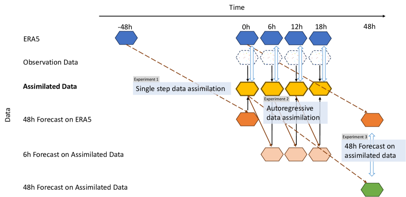
Figure 3: Overview of the experiment settings. Hexagon represents atmosphere states, black arrow represents data assimilation, brown solid arrow represents 6h forecast, brown dashed arrow represents 48h forecast, hexagon with dashed edges and sparse points represent sparse observations, and wide arrow represents target and reference in each experiment. Forecast using GraphCast takes in atmosphere states at two time steps, this is ignored in this diagram for simplicity.

We demonstrate the effectiveness of our method by performing real-world inspired experiments with increasing complexity (Figure 3). In the basic scenario, we perform data assimilation on 48h forecast and observation data, then directly compare the assimilated data with the ground truth data. Furthermore, we evaluate our method with autoregressive data assimilation where the predicted state is produced by a 6h forecast from the assimilated state 6 hour ago. We design this experiment to test whether the assimilate data will deviate from the ground truth data, which is crucial in real world applications. We also designed another experiment to compare the 48h forecast result based on assimilated data and ground truth data, and evaluate the effect of data assimilation method on the forecast skill.

In all the experiments, observations are simulated by taking random columns from the ERA5 dataset considered as the ground truth. We vary the number of observed columns $m$ in the experiments from 1,000 to 40,000 to test the convergence property of our data assimilation method.

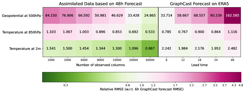
Figure 4: Root mean square error (RMSE) of geopotential at 500hPa, temperature at 850hPa, and temperature at 2m from the single step assimilated data and GraphCast forecast data (shown by the numbers in the cell). The error is calculated against the ERA5 data. The cells are color-coded with the RMSE relative to the 6h forecast RMSE where green means better and red means worse.

Single step data assimilation

In this experiment, we perform data assimilation with a 48h GraphCast forecast and observed columns from 1,000 to 40,000, calculate the error between the assimilated data and the ground truth data, and compare this error against forecast errors with lead times from 6h to 48h.

The result is presented in Figure 4 where we pick three representative variables closely related with forecast skills [Ashkboos et al., 2022, Rasp et al., 2020] including geopotential at 500hPa (z500), temperature at 850hPa (t850), and temperature at 2m (t2m) as the variable. With only 1,000 observed columns ($<0.1\%$ total columns), the assimilated data already achieves a lower RMSE compared to the input 48h forecast data for z500 and t850, while the error of t2m is even lower than the 6h forecast. The error further decreases as the number of observed columns increases. On the other side of the spectra, with 40,000 observed columns ($<3.9\%$ total columns), the RMSE of all three variables are lower than the 6h forecast error. This indicates our assimilation method can indeed improve over the given predicted state and converges to the ground truth as the number of observed columns increases.

Autoregressive data assimilation

In an operational data assimilation system, data assimilation is performed in an autoregressive way: assimilated data from previous time steps are used for producing forecast at the next time step which is in turn used for assimilating data at that time step. Following the operational setting, we perform autoregressive data assimilation cycle: it starts from a 48h forecast at 0h, and repeat the data assimilation - 6h forecast cycle autoregressively. In the data assimilation cycle, two strategies of sampling the columns are used. One is to sample the columns at the same locations (Figure 5). The other resamples data at different locations in each iteration (Figure 6). The strategies helps estimate the performance in real-world cases since the reality is the mix of the two strategies where some observations are measured at the same locations such as weather stations and geostationary satellites, while locations of other observations change with time. We evaluate the autoregressive data assimilation result similar to the previous experiment.

In the results, we observed distinct patterns for fixed and non-fixed sampling strategies. With fixed sampling (Figure 5), the initial five iterations showed promising performance, but an error began to accumulate in subsequent iterations. Notably, this error demonstrated a diurnal pattern in the assimilation error for temperature at 2 meters (t2m). In contrast, the non-fixed sampling strategy showed a slower rate of error accumulation compared to fixed sampling (Figure 6). However, a significant issue was identified in both strategies: the assimilated error (solid lines) consistently exceeded the interpolation error (dash lines) after several iterations. This outcome suggests that our assimilation method is not effectively utilizing the input observational data to its full potential.

Figure 5: RMSE of geopotential at 500hPa, temperature at 850hPa and temperature at 2m from autoregressively assimilated data (solid lines) and interpolated observations (dash lines). The observations at made at the same locations in each assimilation step.

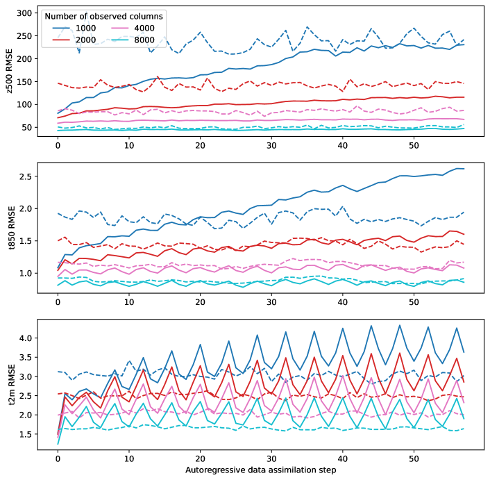
Figure 6: RMSE of geopotential at 500hPa, temperature at 850hPa and temperature at 2m from autoregressively assimilated data (solid lines) and interpolated observations (dash lines). The observations are made at different locations in each assimilation step.

Forecast on single step data assimilation result

Since assimilated data is often used as the input of weather forecasts, it is important to test the forecast error using our assimilated data. In this experiment, we perform data assimilation at 0h, perform a 48h GraphCast forecast, then compare the forecast error again error of forecasts with varying lead times using ERA5 at 0h as inputs.

Figure 7: Root mean square error (RMSE) of geopotential at 500hPa, temperature at 850hPa, and temperature at 2m from the 48h forecast using assimilated data as inputs and forecasts with lead times from 48h to 78h using ERA5 as inputs (shown by the numbers in the cell). The error is calculated against the ERA5 data. The cells are color-coded with the RMSE relative to the 72h forecast RMSE where green means better and red means worse.

As the score board plot in Figure 7 shows, results from this experiment reveal that the 48h forecast error using assimilated data inputs gradually converges to the 48h forecast errors using ERA5 inputs. The error using assimilated data cannot be lower than using ERA5 inputs because the ERA5 data is used to emulate observations in the experiment. However, this setup allows us to compare the forecast error against forecasts with longer lead times to determine the extent of lead time lost due to the use of assimilated data as forecast inputs. With 8,000 observed columns, the error for z500, t850, and t2m is lower than the 72h forecast error. This implies that the lead time lost is less than 24 hours. With 40,000 observed columns, the error for z500 and t850 is approximately equivalent to the 54h forecast error. However, the t2m error remains larger than the 60h forecast error, potentially due to diurnal effects that cause a decrease in the forecast error of t2m from a 48h to a 60h lead time.

3.5 Conclusion

In summary, we propose a data assimilation method capable of assimilating high-resolution atmospheric variables using predicted state and sparse observations. Our approach is based on the denoising diffusion model, which is able to sample from conditional probability distributions. Notably, we adapted the pretrained GraphCast weather forecast model as the denoising model motivated by its compatible input and output shapes. Our method’s flexibility also allows for the possibility of integrating other forecast models, ensuring ease of updates and maintenance.

A key feature of our method is the enforcement of conditioning on the predicted state during both training and inference periods, and the conditioning of sparse observations exclusively at the inference stage. An additional benefit of this conditioning approach is the automatic generation of a post-processing model, should observations not be supplied at inference time.

Our experimental results validated the effectiveness of this approach: we observed that the assimilated data converges to the observations. When used as an input for forecast models, assimilated data resulted in a maximum lead time loss of 24 hours. Furthermore, when provided with sufficient observations, our method proved to be capable of producing reanalysis data.

Limitations

Currently, our method lacks a 4D assimilation capability and is unable to assimilate observations other than direct point measurements of assimilated variables. We are working on assimilating point observations at multiple time steps as well as general observations such at satellite imagery and radar soundings. The columns of ERA5 that are used as mock observations within this study are easier to use as they hold less uncertainty when compared to real observations that suffer from measurement errors. However, there are overall many more observations available in real-world forecasts when compare to the number use in this paper.

4 Acknowledgements

This study received funding from the MAELSTROM project funded by the European High-Performance Computing Joint Undertaking (JU; grant agreement No 955513).

References

- ipc [2023] page 35–144. Cambridge University Press, July 2023. ISBN 9781009157896. doi: 10.1017/9781009157896.002. URL http://dx.doi.org/10.1017/9781009157896.002.
- Andry et al. [2023] G. Andry et al. Data assimilation as simulation-based inference. 2023.
- Andrychowicz et al. [2023] M. Andrychowicz, L. Espeholt, D. Li, S. Merchant, A. Merose, F. Zyda, S. Agrawal, and N. Kalchbrenner. Deep learning for day forecasts from sparse observations. arXiv preprint arXiv:2306.06079, 2023.
- Ashkboos et al. [2022] S. Ashkboos, L. Huang, N. Dryden, T. Ben-Nun, P. Dueben, L. Gianinazzi, L. Kummer, and T. Hoefler. Ens-10: A dataset for post-processing ensemble weather forecasts. Advances in Neural Information Processing Systems, 35:21974–21987, 2022.
- Bannister [2017] R. N. Bannister. A review of operational methods of variational and ensemble-variational data assimilation. Quarterly Journal of the Royal Meteorological Society, 143(703):607–633, 2017.
- Bi et al. [2023] K. Bi, L. Xie, H. Zhang, X. Chen, X. Gu, and Q. Tian. Accurate medium-range global weather forecasting with 3d neural networks. Nature, 619(7970):533–538, 2023.
- Bonavita et al. [2016] M. Bonavita, E. Hólm, L. Isaksen, and M. Fisher. The evolution of the ecmwf hybrid data assimilation system. Quarterly Journal of the Royal Meteorological Society, 142(694):287–303, 2016.
- Bradbury et al. [2018] J. Bradbury, R. Frostig, P. Hawkins, M. J. Johnson, C. Leary, D. Maclaurin, G. Necula, A. Paszke, J. VanderPlas, S. Wanderman-Milne, and Q. Zhang. JAX: composable transformations of Python+NumPy programs, 2018. URL http://github.com/google/jax.
- Chung et al. [2022] H. Chung, J. Kim, M. T. Mccann, M. L. Klasky, and J. C. Ye. Diffusion posterior sampling for general noisy inverse problems. In The Eleventh International Conference on Learning Representations, 2022.
- Evensen et al. [2022] G. Evensen, F. C. Vossepoel, and P. J. van Leeuwen. Data assimilation fundamentals: A unified formulation of the state and parameter estimation problem. Springer Nature, 2022.
- Finn et al. [2023] T. S. Finn, L. Disson, A. Farchi, M. Bocquet, and C. Durand. Representation learning with unconditional denoising diffusion models for dynamical systems. EGUsphere, 2023:1–39, 2023.
- Hersbach et al. [2020] H. Hersbach, B. Bell, P. Berrisford, S. Hirahara, A. Horányi, J. Muñoz-Sabater, J. Nicolas, C. Peubey, R. Radu, D. Schepers, et al. The era5 global reanalysis. Quarterly Journal of the Royal Meteorological Society, 146(730):1999–2049, 2020.
- Ho et al. [2020] J. Ho, A. Jain, and P. Abbeel. Denoising diffusion probabilistic models. Advances in neural information processing systems, 33:6840–6851, 2020.
- Lam et al. [2023] R. Lam, A. Sanchez-Gonzalez, M. Willson, P. Wirnsberger, M. Fortunato, F. Alet, S. Ravuri, T. Ewalds, Z. Eaton-Rosen, W. Hu, et al. Learning skillful medium-range global weather forecasting. Science, page eadi2336, 2023.
- Law et al. [2015] K. Law, A. Stuart, and K. Zygalakis. Data assimilation. Cham, Switzerland: Springer, 214:52, 2015.
- Li et al. [2023] L. Li, R. Carver, I. Lopez-Gomez, F. Sha, and J. Anderson. Seeds: Emulation of weather forecast ensembles with diffusion models. arXiv preprint arXiv:2306.14066, 2023.
- Loshchilov and Hutter [2018] I. Loshchilov and F. Hutter. Fixing weight decay regularization in adam. 2018.
- Lugmayr et al. [2022] A. Lugmayr, M. Danelljan, A. Romero, F. Yu, R. Timofte, and L. Van Gool. Repaint: Inpainting using denoising diffusion probabilistic models. In Proceedings of the IEEE/CVF Conference on Computer Vision and Pattern Recognition, pages 11461–11471, 2022.
- Mardani et al. [2023] M. Mardani, N. Brenowitz, Y. Cohen, J. Pathak, C.-Y. Chen, C.-C. Liu, A. Vahdat, K. Kashinath, J. Kautz, and M. Pritchard. Generative residual diffusion modeling for km-scale atmospheric downscaling. arXiv preprint arXiv:2309.15214, 2023.
- Mardani et al. [2024] M. Mardani, N. Brenowitz, Y. Cohen, J. Pathak, C.-Y. Chen, C.-C. Liu, A. Vahdat, K. Kashinath, J. Kautz, and M. Pritchard. Residual diffusion modeling for km-scale atmospheric downscaling. 2024.
- Pathak et al. [2022] J. Pathak, S. Subramanian, P. Harrington, S. Raja, A. Chattopadhyay, M. Mardani, T. Kurth, D. Hall, Z. Li, K. Azizzadenesheli, et al. Fourcastnet: A global data-driven high-resolution weather model using adaptive fourier neural operators. arXiv preprint arXiv:2202.11214, 2022.
- Price et al. [2023] I. Price, A. Sanchez-Gonzalez, F. Alet, T. Ewalds, A. El-Kadi, J. Stott, S. Mohamed, P. Battaglia, R. Lam, and M. Willson. Gencast: Diffusion-based ensemble forecasting for medium-range weather. arXiv preprint arXiv:2312.15796, 2023.
- Rasp et al. [2020] S. Rasp, P. D. Dueben, S. Scher, J. A. Weyn, S. Mouatadid, and N. Thuerey. Weatherbench: a benchmark data set for data-driven weather forecasting. Journal of Advances in Modeling Earth Systems, 12(11):e2020MS002203, 2020.
- Rasp et al. [2023] S. Rasp, S. Hoyer, A. Merose, I. Langmore, P. Battaglia, T. Russel, A. Sanchez-Gonzalez, V. Yang, R. Carver, S. Agrawal, et al. Weatherbench 2: A benchmark for the next generation of data-driven global weather models. arXiv preprint arXiv:2308.15560, 2023.
- Rozet and Louppe [2023a] F. Rozet and G. Louppe. Score-based data assimilation. arXiv preprint arXiv:2306.10574, 2023a.
- Rozet and Louppe [2023b] F. Rozet and G. Louppe. Score-based data assimilation for a two-layer quasi-geostrophic model. arXiv preprint arXiv:2310.01853, 2023b.
- Saharia et al. [2022] C. Saharia, W. Chan, S. Saxena, L. Li, J. Whang, E. L. Denton, K. Ghasemipour, R. Gontijo Lopes, B. Karagol Ayan, T. Salimans, et al. Photorealistic text-to-image diffusion models with deep language understanding. Advances in Neural Information Processing Systems, 35:36479–36494, 2022.
- Song et al. [2020] Y. Song, J. Sohl-Dickstein, D. P. Kingma, A. Kumar, S. Ermon, and B. Poole. Score-based generative modeling through stochastic differential equations. arXiv preprint arXiv:2011.13456, 2020.
- Virtanen et al. [2020] P. Virtanen, R. Gommers, T. E. Oliphant, M. Haberland, T. Reddy, D. Cournapeau, E. Burovski, P. Peterson, W. Weckesser, J. Bright, et al. Scipy 1.0: fundamental algorithms for scientific computing in python. Nature methods, 17(3):261–272, 2020.