Stereographic Projections for Designs on the Sphere

Abstract

This paper is concerned with the use of the stereographic projection in order to map the sphere points of designs for regression models in three variables and design space the unit ball onto the two-dimensional stereogram. Details of the projection and its attendant stereogram are given. Stereograms which represent the spherical component of designs with points on the sphere and the centre of the unit ball, including the central composite and the Box-Behnken designs, are introduced. In addition, an example in which stereograms are used to elucidate the geometric isomorphism of a suite of designs generated by an exchange algorithm is presented.

1 Introduction

Designs over the unit ball which comprise a finite set of support points have been reported sporadically in the literature as, for example, in the papers of Bose and Draper (1959), Hardin and Sloane (1991), Gilmour (2006), Dette and Grigoriev (2014), Hirao et al. (2015) and Radloff and Schwabe (2023). The designs are not straightforward to construct and, to compound matters, the three-dimensional prototypes, which help to convey the innate structure of the designs, are not easy to represent on paper. The aim of the present study therefore is to introduce the stereographic projection as a valuable tool, in research and pedagogically, for representing the spherical components of designs in three independent variables over the unit ball in two dimensions. The paper is organized as follows. The notion of the stereographic projection and the construction of the attendant stereogram are presented in Section 2. Illustrative examples relating to the quadratic polynomial model in three variables are then provided in Section 3. Some general comments on the relevance of the use of the stereographic projection in experimental design are presented in Section 4.

2 The Stereographic Projection

Consider first a perfect terrestrial globe which is centred at the origin with the North-South axis oriented vertically and the equatorial plane perpendicular to that axis. The stereographic projection maps points and circles on the three-dimensional globe onto the two-dimensional equatorial plane, with the resulting construct termed a stereogram. In particular, consider a point lying on the surface of the globe in the northern hemisphere. Then a line can be drawn from that point to the South Pole and the point of intersection of the line with the equatorial plane indicated on the stereogram with a solid circle, as shown in Figure 1(a). Similarly, a line can be drawn from a point on the surface of the globe in the southern hemisphere to the North Pole and its intersection with the equatorial plane denoted for clarity by an open circle, as in Figure 1(b). In addition, parallels, that is lines of latitude, are projected onto the equatorial plane as circles centred at the origin and meridians, that is lines of longitude, as straight lines through the origin. These constructs can be represented by a polar net, as shown in Figure 1(c). Great circles through two points on the surface of the sphere can also be projected onto the equatorial plane, specifically as arcs with diagonally opposite end points touching the equator. Selected meridians and great circles are shown on the stereogram in Figure 1(d).

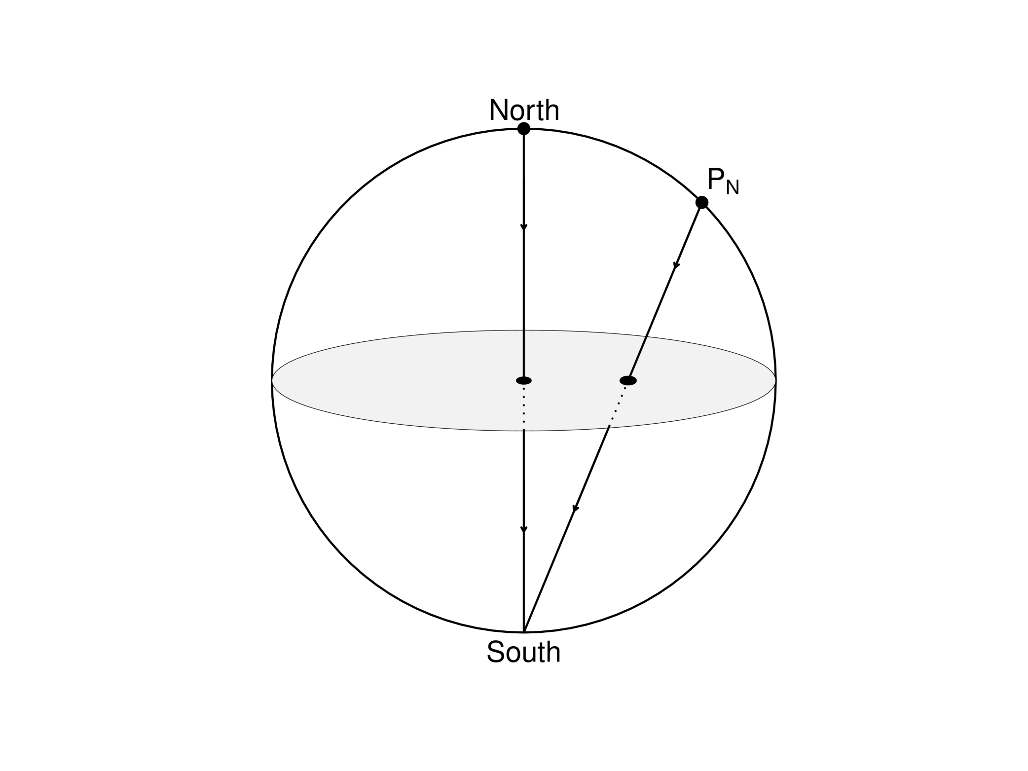
(a) Northern Hemisphere

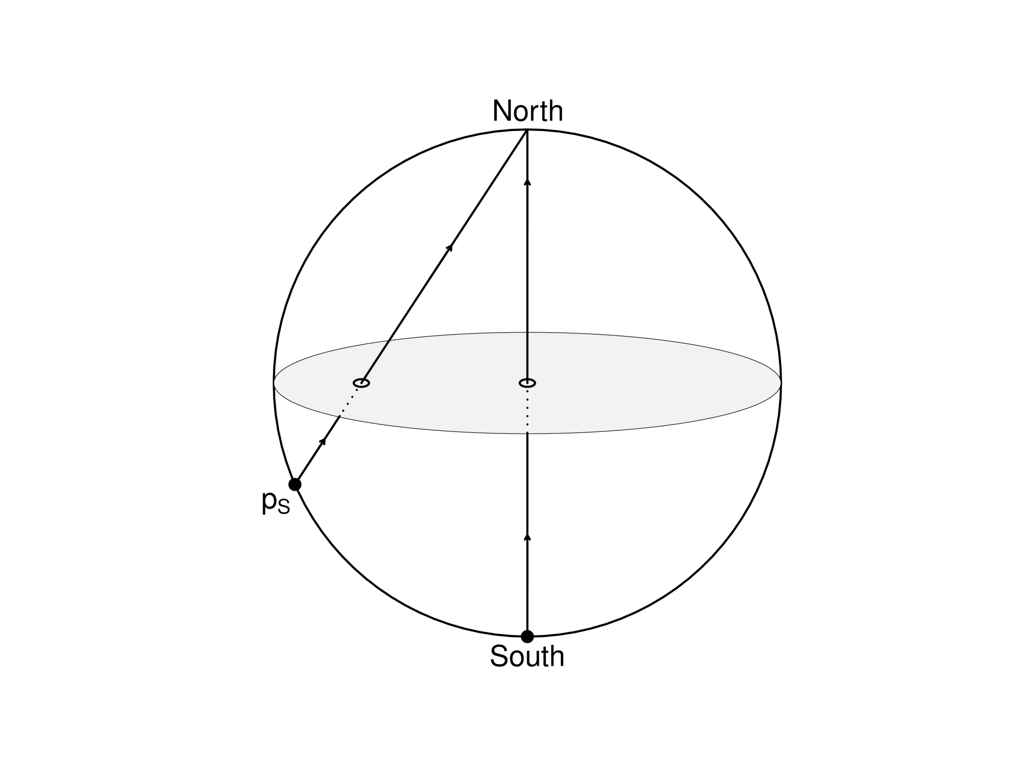
(b) Southern Hemisphere

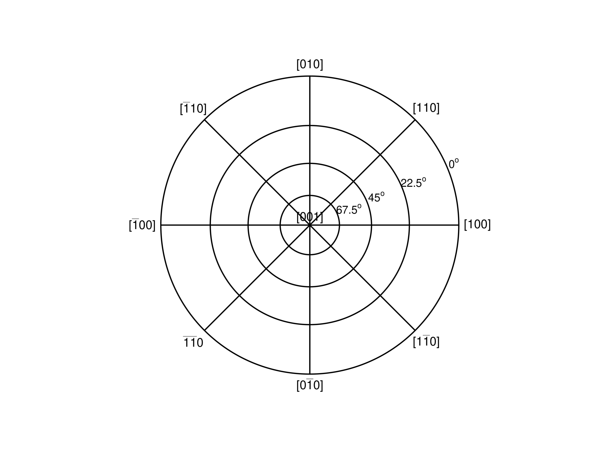
(c) Meridians and Parallels

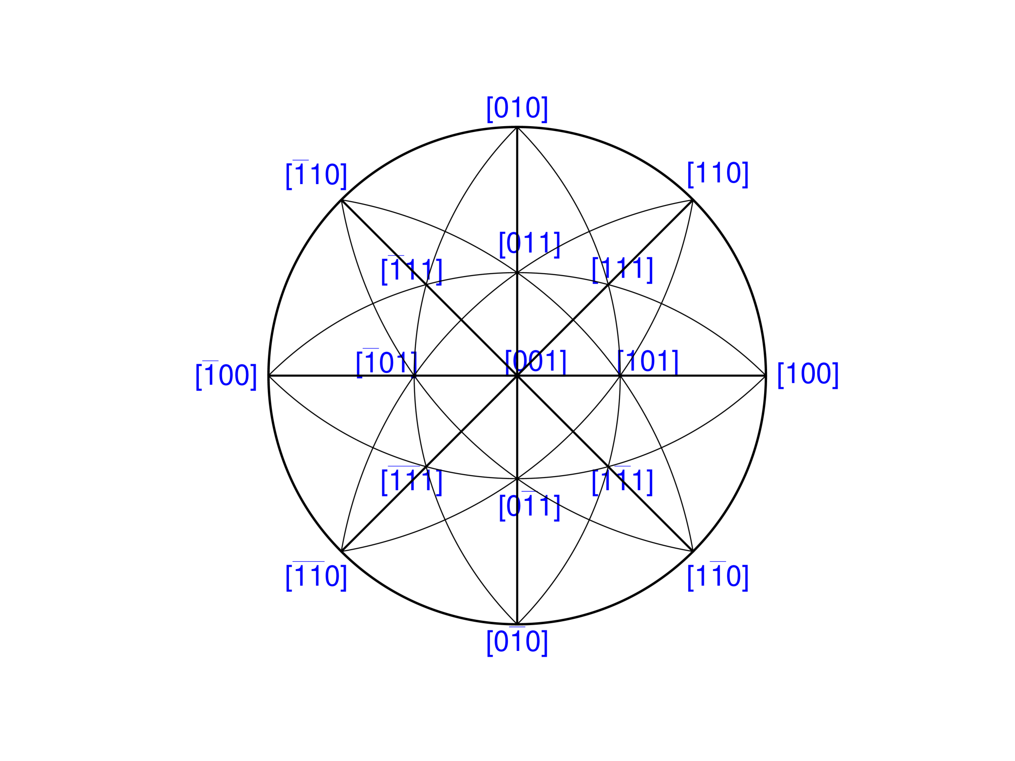
(d) Meridians and Great Circles

Figure 1: Stereographic projections for points (a) in the northern hemisphere and (b) in the southern hemisphere. Stereograms, looking down the North-South axis, of (c) meridians and parallels and (d) meridians and great circles.

Three-dimensional directions are often indicated on the stereogram and, for example, the vectors $(1,1,1)$ and $(-1,1,0)$ are denoted compactly by $[111]$ and $[\bar{1}10]$. To give a sense of the orientation of the equatorial plane, selected directions are included in Figure 1(d). Finally, note that a small circle drawn on the surface of the globe can be projected as a circle onto the stereogram but the centres of the two circles do not necessarily correspond. Further details on the stereographic projection are given, for example, in the books on crystallography by Borchardt-Ott (2011), De Graef and McHenry (2012) and Hammond (2015).

The stereographic projection can now be adapted to accommodate designs in three dimensions on design space the unit ball with centre at the origin and support points on the boundary and at the centre of the ball. Specifically, consider the perfect terrestrial globe described above as a unit sphere with a right-handed coordinate system specified by the coordinates $x_{1},x_{2}$ and $x_{3}$. Then the point $(0,0,1)$ can be taken taken to coincide with the North Pole, the point $(0,1,0)$ with the intersection of a line in the direction $[0,1,0]$ with the equator and the $(x_{1},x_{2})$-plane with the equatorial plane. The support points of a design on the surface of the sphere can be projected onto the equatorial plane, that is the stereogram, by invoking the mapping $(x_{1},x_{2},x_{3})\mapsto\big{(}\displaystyle\frac{x_{1}}{1+|x_{3}|},\frac{x_{2}}{1+|x_{3}|}\big{)}$. Projections onto the stereogram of the appropriate meridians and great circles which connect the design points then follow.

3 Examples

3.1 Subset Designs

To fix ideas, consider the subset designs for the quadratic polynomial model with three independent variables over the unit ball ntroduced into the literature in the paper by Gilmour (2006). The support points of the designs lie on the surface and at the centre of the unit ball and are taken from the sets specified by

$$S_{0}=(0,0,0),~{}S_{1}=(\pm 1,0,0)_{\mathrm{\small cycle}},~{}S_{2}=(\pm\frac{1}{\sqrt{2}},\pm\frac{1}{\sqrt{2}},0)_{\mathrm{\small cycle}},~{}S_{3}=(\pm\frac{1}{\sqrt{3}},\pm\frac{1}{\sqrt{3}},\pm\frac{1}{\sqrt{3}})$$

which comprise $1,6,12$ and $8$ points respectively. The subscript ‘cycle’ indicates that the three coordinates of the points can be moved cyclically. More specifically, subset designs can be expressed as a linear combination of these sets of points, that is as $c_{0}S_{0}+c_{1}S_{1}+c_{2}S_{2}+c_{3}S_{3}$, where $c_{0}>0$ and the remaining coefficients, $c_{1},c_{2}$ and $c_{3}$, are greater than or equal to zero and are chosen in such a way that the moment matrix is nonsingular. From a symmetry perspective, the sets of points $S_{0},S_{1},S_{2}$ and $S_{3}$ correspond to the centre point and, for a cube inscribed in the unit sphere, to the intersection of the six normals to the faces of the cube with the sphere, to the intersection of the 12 lines from the origin through the mid-points of the edges of the cube with the sphere, and to the eight vertices of the cube itself, respectively. It thus follows that the points on the unit sphere of a subset design with equal weights assigned to the subsets $S_{1},S_{2}$ and $S_{3}$ belong to the point group $O_{h}$.

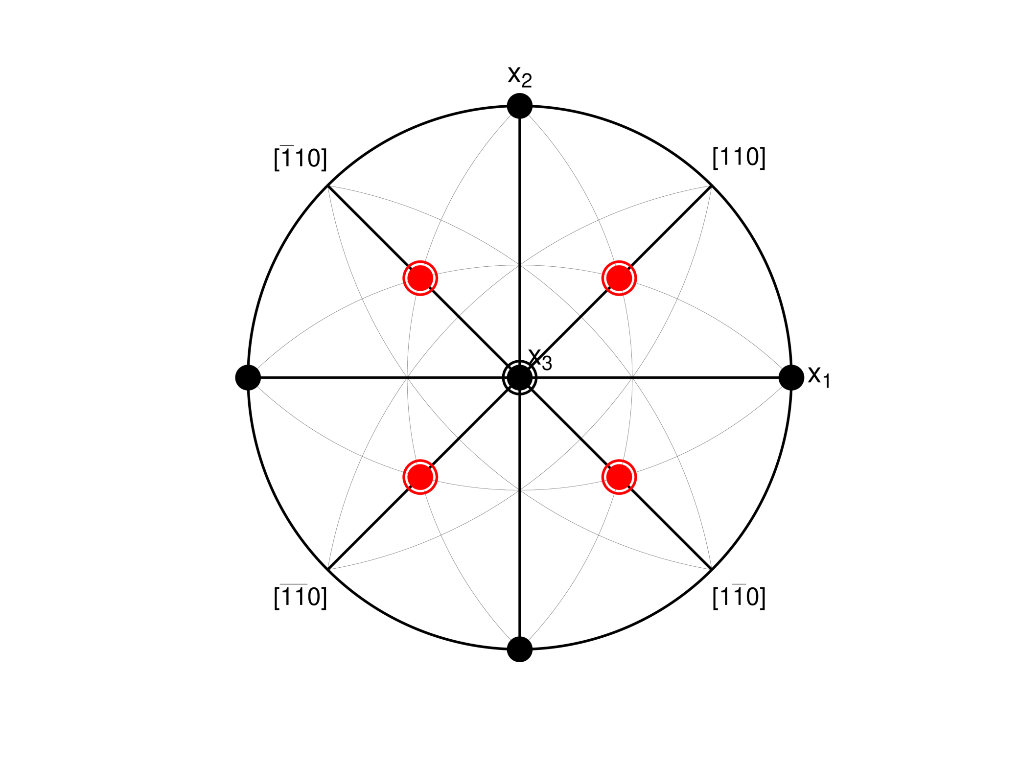
(a) Central Composite Design

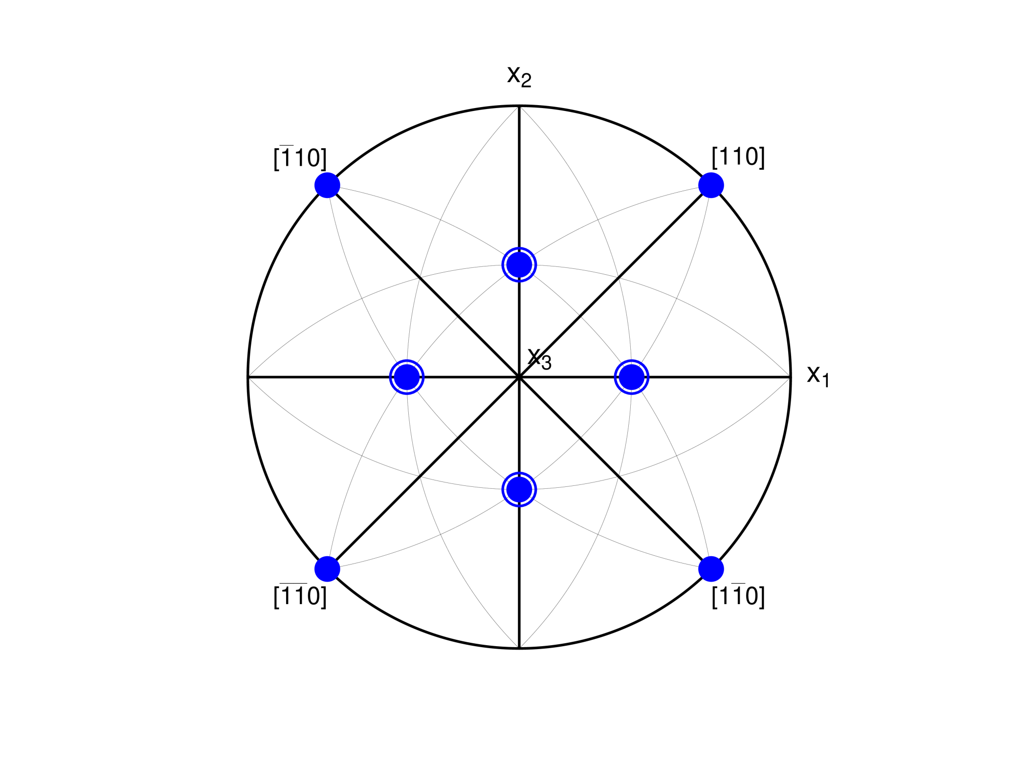
(b) Box-Behnken Design

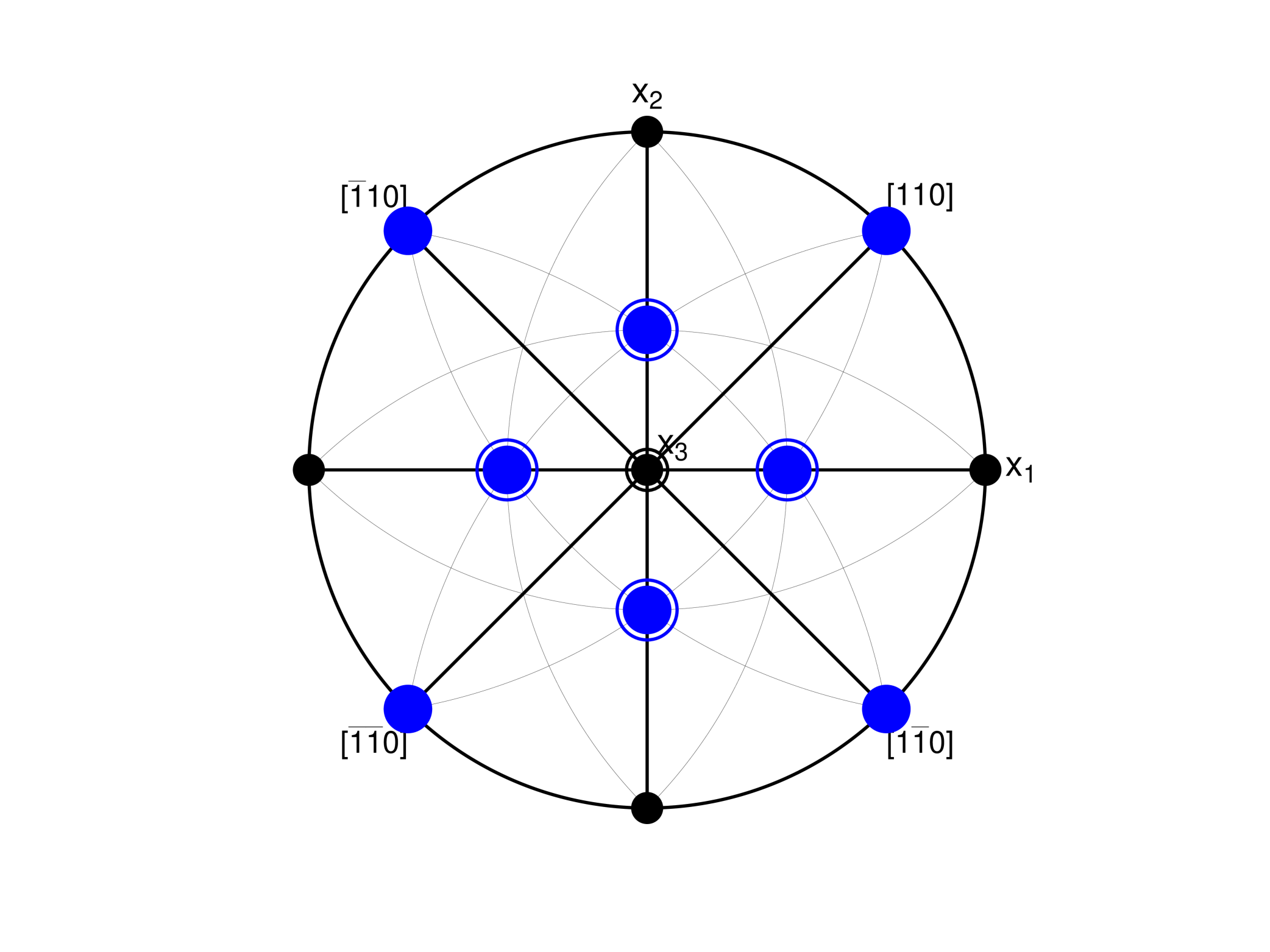
(c) Rotatable Design

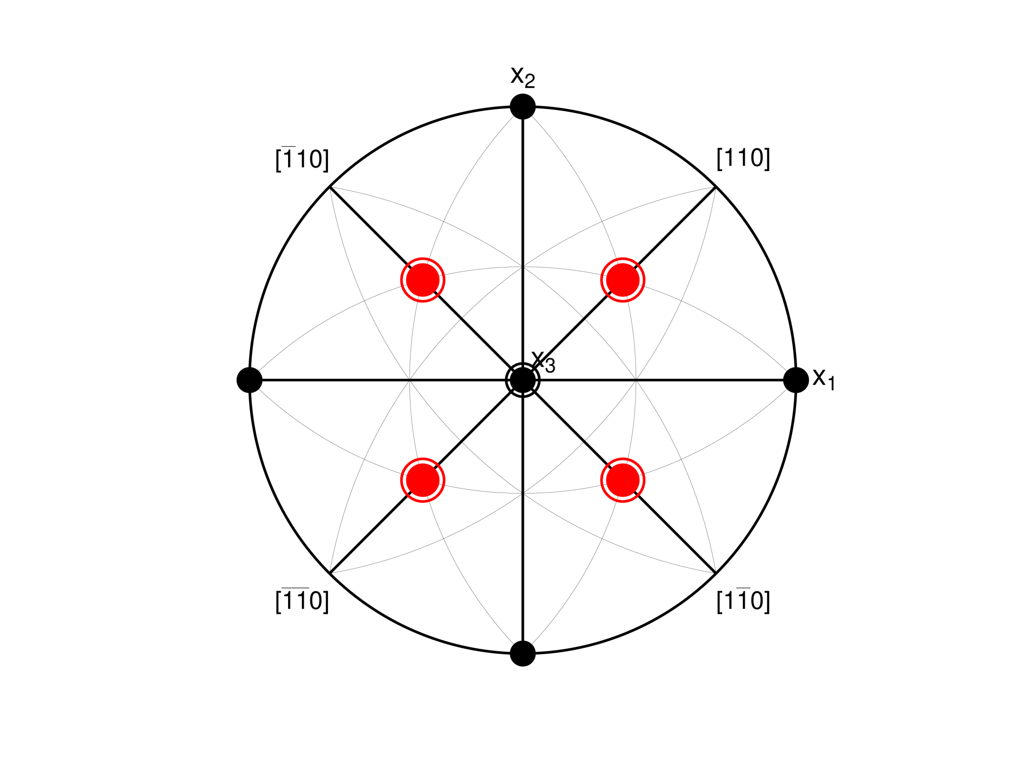
(d) Approximate $E$-optimal Design

Figure 2: Stereograms of the sphere points of (a) the central composite design, (b) the Box-Behnken design, (c) the rotatable design $S_{0}+S_{1}+2S_{2}$ and (d) the approximate $E$-optimal design $\frac{9}{17}S_{0}+\frac{3}{17}S_{1}+\frac{5}{17}S_{3}$. In (c) and (d) the areas of the solid circles are proportional to the relative weightings of the points on the sphere.

The central composite design over design space the unit ball is the subset design $S_{0}+S_{1}+S_{3}$ and the stereographic projection of the 14 design points on the sphere yields the stereogram shown in Figure 2(a). Similarly, the Box-Behnken design is the subset design $S_{0}+S_{2}$ and the stereogram of the 12 points on the sphere is shown in Figure 2(b). Note that the points in $S_{1},S_{2}$ and $S_{3}$ are coloured in the stereograms in black, blue and red, respectively, in Figure 2 and that the complementary relationship between the two designs is clearly illustrated by the stereograms. Subset designs with different coefficients allocated to the sets of points $S_{0},S_{1},S_{2}$ and $S_{3}$ can also be represented compactly on a stereogram by using colour-coding and points with areas proportional to their relative weightings. For example, the subset design $S_{0}+S_{1}+2S_{2}$ is rotatable and the different allocations of points to the two sets $S_{1}$ and $S_{2}$ is highlighted in the stereogram in Figure 2(c). In addition, the approximate $E$-optimal design for the quadratic polynomial model in three variables on the unit ball derived by Dette and Grigoriev (2014) is the subset design $\frac{9}{17}S_{0}+\frac{3}{17}S_{1}+\frac{5}{17}S_{3}$ and thus a weighted form of the central composite design. The stereogram of the sphere points of the design and their relative weighting is shown in Figure 2(d). Note that the design itself is rather curious in that more than half of the weight is placed on the centre point.

3.2 An Application

Gilmour and Trinca (2012), in Example 2 of their paper, considered optimal designs which accommodate inference for a full quadratic polynomial model in three independent variables with support points on the surface and at the centre of a ball with radius 3. For clarity, their results are reported here for the unit ball. The authors focussed on nonsingular designs with 18 support points taken, with replacement, from the $27$ individual points belonging the subsets $S_{0},S_{1},S_{2}$ and $S_{3}$ of the previous example. More specifically, they considered, inter alia, D_S-optimal designs which minimise the volume of the confidence region for the parameters of the model with the intercept treated as a nuisance parameter and (DP)_S-optimal designs which minimise the D_S-criterion multiplied by an appropriate quantile of the $F$-distribution raised to the power equal to the number of parameters of interest, in this case nine. It can in fact be easily shown that over $3\times 10^{10}$ possible designs must be enumerated in order to identify those designs which are strictly D_S- and (DP)_S-optimal. As a consequence, Gilmour and Trinca (2012) used a heuristic, the exchange algorithm documented in, for example, Atkinson et al. (2007), to search for designs which are optimal or near-optimal.

The question now arises as to how many strictly D_S- and (DP)_S-optimal designs are generated by the exchange algorithm and, if more than one, how the resultant designs are related. This question in turn impacts on the performance of the algorithm. To this end, the exchange procedure of Gilmour and Trinca (2012) was run five million times in the programming language gauss (2022) and the requisite optimal designs which were distinct, that is non-coincident, identified. Eight distinct D_S-optimal designs with two centre points and $1,080$ distinct (DP)_S-optimal designs, with $216$ including a single centre point and $864$ two centre points, were so generated. The designs were then examined in the context of isomorphism and, since the factors $0,1,\frac{1}{\sqrt{2}}$ and $\frac{1}{\sqrt{3}}$ are quantitative, in that of geometric isomorphism (Cheng and Ye 2004). Specifically, two designs are said to be geometrically isomorphic if the designs can be obtained, one from the other, by rotations and reflections within the design space. In the present example, the isomorphic properties of the designs are determined solely by the spherical points and the actions of rotation and reflection can therefore be mapped, albeit indirectly, onto the stereograms. It is crucial to observe here that a design which is geometrically isomorphic to a D_S-optimal or a (DP)_S-optimal design is itself necessarily D_S-optimal or (DP)_S-optimal.

The D_S-optimal design given in Table 2 of Gilmour and Trinca (2012) comprises 16 points on the sphere, none of which are replicated, and two centre points, and coincides with one of the eight distinct D_S-optimal designs generated by the exchange algorithm. The stereogram of the spherical points of the design is presented in Figure 3(a), with the great circles introduced as guidelines for the placement of the points. It is immediately clear from the figure that a further three distinct designs can be generated from the design by repeated rotations through $90^{\circ}$ about the $x_{3}$ axis and the associated stereograms are shown in Figures 3(b), 3(c) and 3(d). A further four designs can then be obtained by reflecting the designs shown in Figure 3 through the plane perpendicular to the $x_{3}$ axis, that is the $(x_{1},x_{2})$-plane. The resultant eight designs so obtained are geometrically isomorphic and therefore D_S-optimal. These isomorphic designs therefore account for the eight distinct D_S-optimal designs generated by the exchange algorithm.

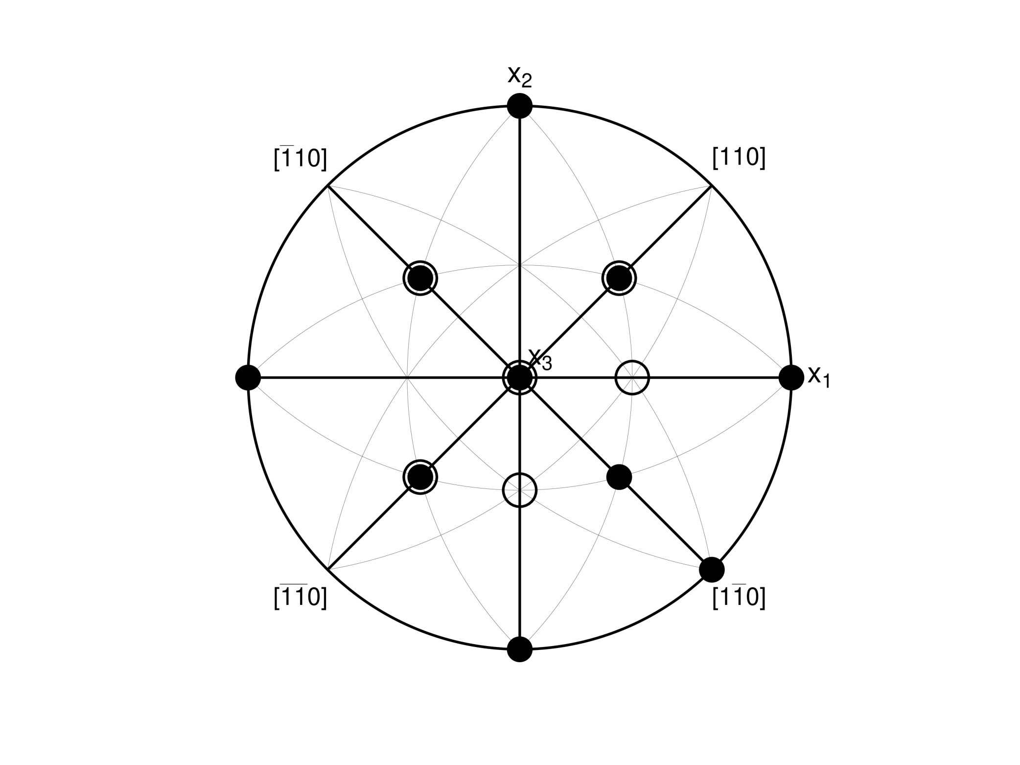
(a) Design of Gilmour and Trinca (2012)

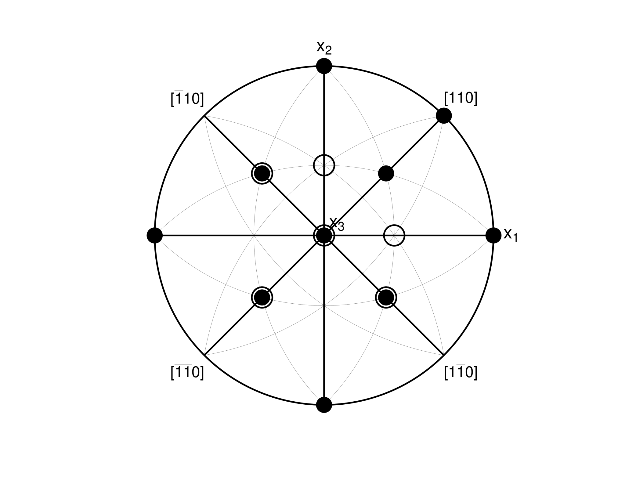
(b) Rotate (a) through $\displaystyle-\frac{\pi}{2}$

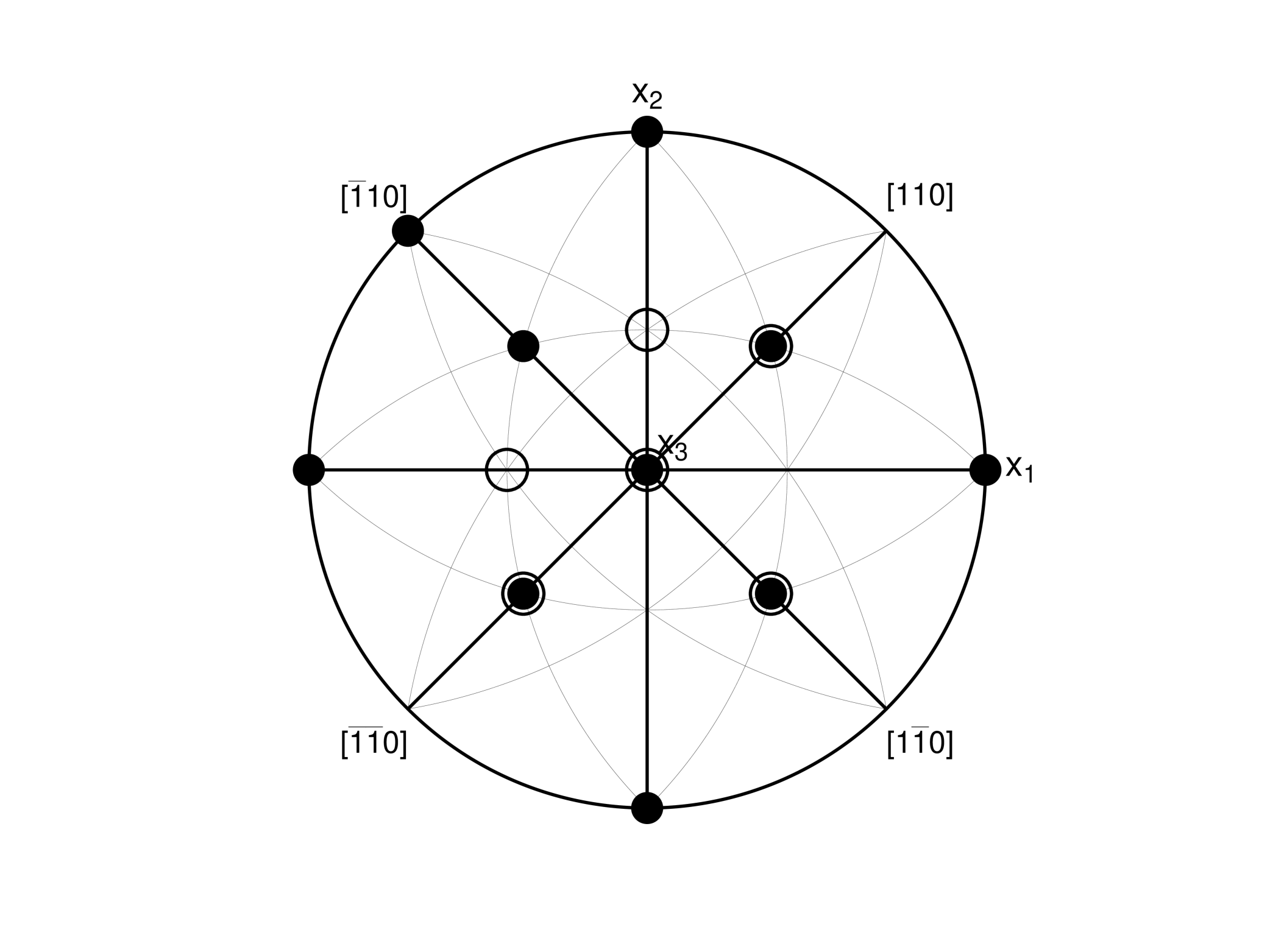
(c) Rotate (b) through $\displaystyle-\frac{\pi}{2}$

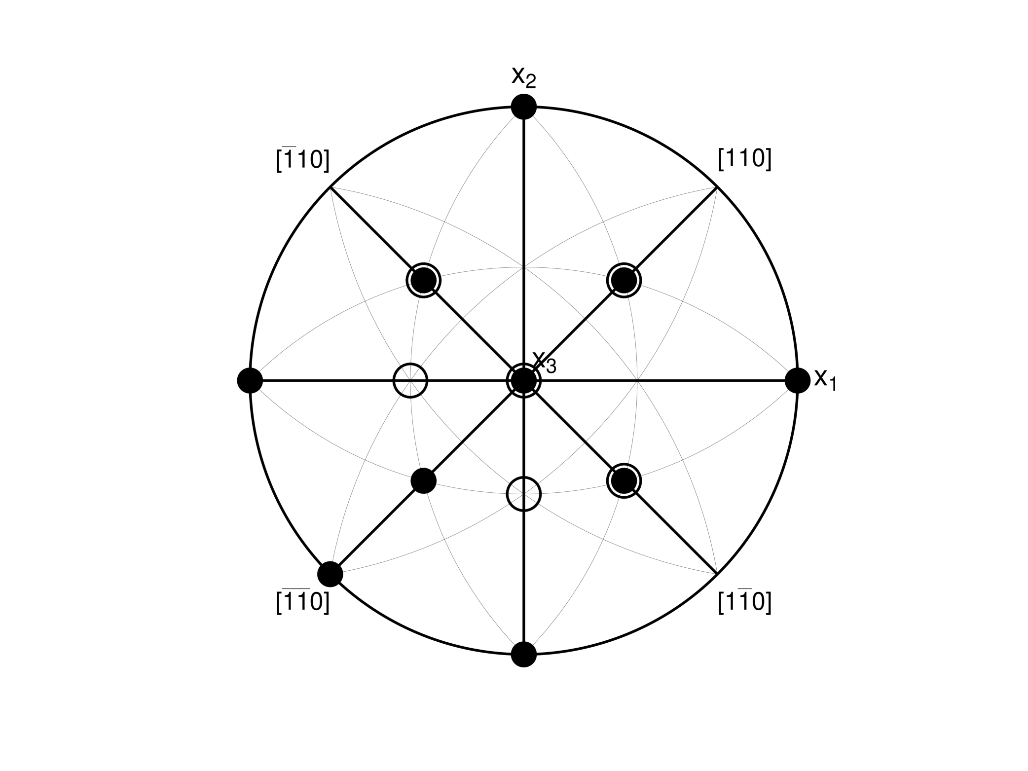
(d) Rotate (c) through $\displaystyle-\frac{\pi}{2}$

Figure 3: Stereograms of exact D_S-optimal designs with (a) the design of Gilmour and Trinca (2012) and (b), (c) and (d) the designs from successive anti-clockwise rotations through 90 degrees about the $x_{3}$-axis, starting with design (a).

The problem of identifying (DP)_S-optimal designs which are geometrically isomorphic from the 1,080 optimal designs generated by the exchange algorithm is a little more nuanced than that relating to the D_S-optimal designs. Consider first the design reported in Table 2 of Gilmour and Trinca (2012) which is easily identified as one of the 216 distinct (DP)_S-optimal designs with a single centre point generated by the exchange algorithm.

This $18$-point design is based on one centre point and on a set of nine distinct points on the sphere, specifically the set

$$B=\left\{(100),(\frac{1}{\sqrt{3}},\pm\frac{1}{\sqrt{3}},-\frac{1}{\sqrt{3}}),(0,\pm\frac{1}{\sqrt{2}},\frac{1}{\sqrt{2}}),(-\frac{1}{\sqrt{2}},0,\pm\frac{1}{\sqrt{2}}),(-\frac{1}{\sqrt{2}},\pm\frac{1}{\sqrt{2}},0)\right\},$$

termed here the basis set, with each point replicated twice except for the point $(-\frac{1}{\sqrt{2}},0,\frac{1}{\sqrt{2}})$ which occurs once. A stereogram of the 17 points on the sphere of the design is presented in Figure 4(a), with the point occurring once indicated in red.

Two distinct designs can be obtained by rotation twice through $180^{\circ}$ about the axis defined by the vector $[1,1,1]$ and are geometrically isomorphic to the original design of Gilmour and Trinca (2012) and therefore (DP)_S-optimal. To illustrate, the stereograms of the two resultant designs are shown in Figures 4(b) and 4(c). As an aside, the designs can also be constructed by cycling the original axes $(x_{1},x_{2},x_{3})$ of Gilmour and Trinca (2012) twice as $(x_{2},x_{3},x_{1})$ and $(x_{3},x_{1},x_{2})$. Eight geometrically isomorphic designs can now be generated from each of the three designs displayed in Figures 4(a), (b) and (c) by rotation through $90^{\circ}$ about the $x_{3}$-axis and reflection about an appropriate plane to yield a total of $3\times 8=24$ designs. The design of Gilmour and Trinca (2012) is therefore representative of a class of 24 geometrically isomorphic designs.

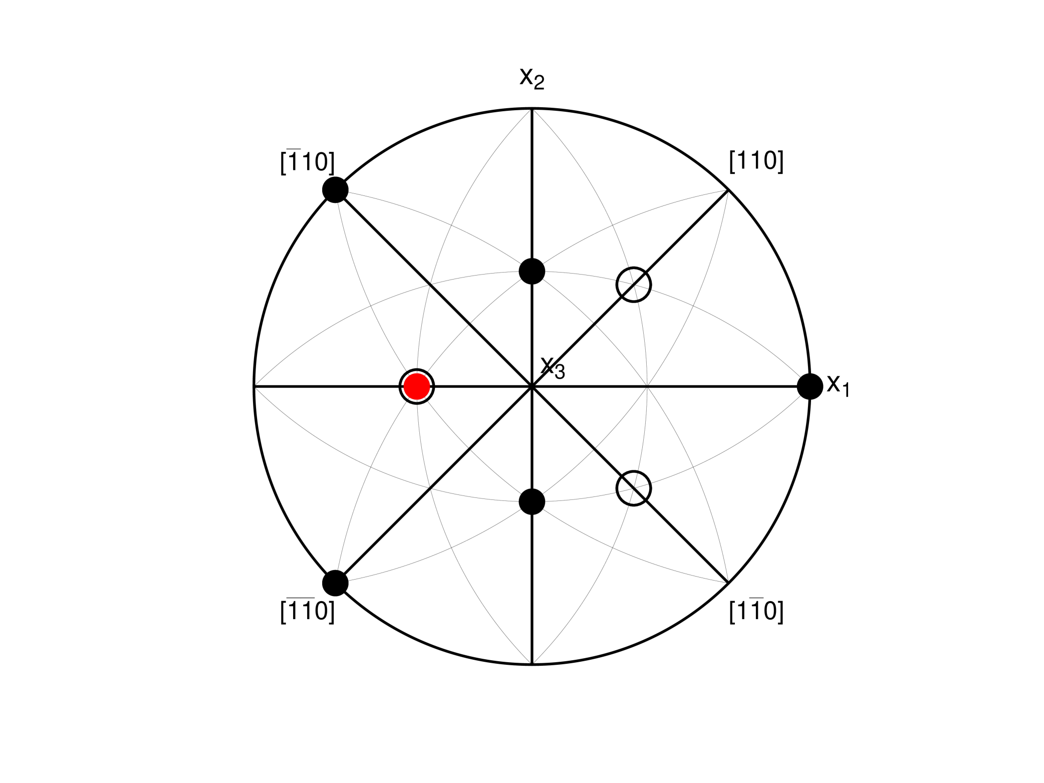
(a) Gilmour and Trinca Design

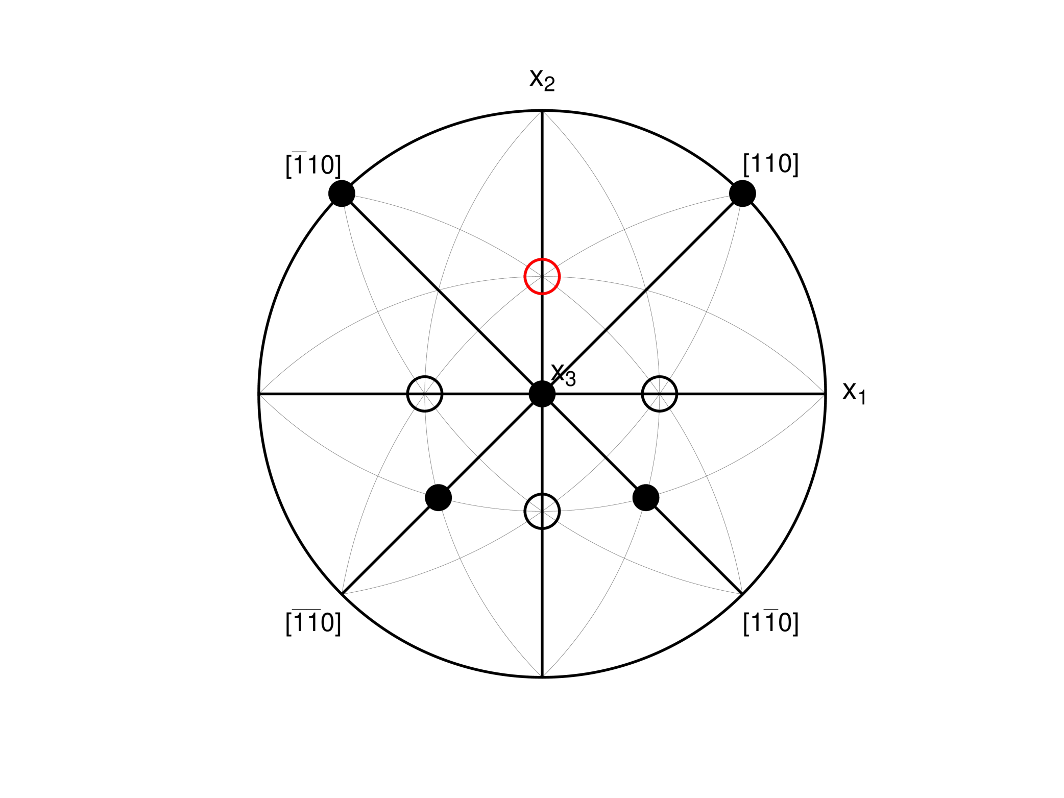
(b) Design 1 Isomorphic to (a)

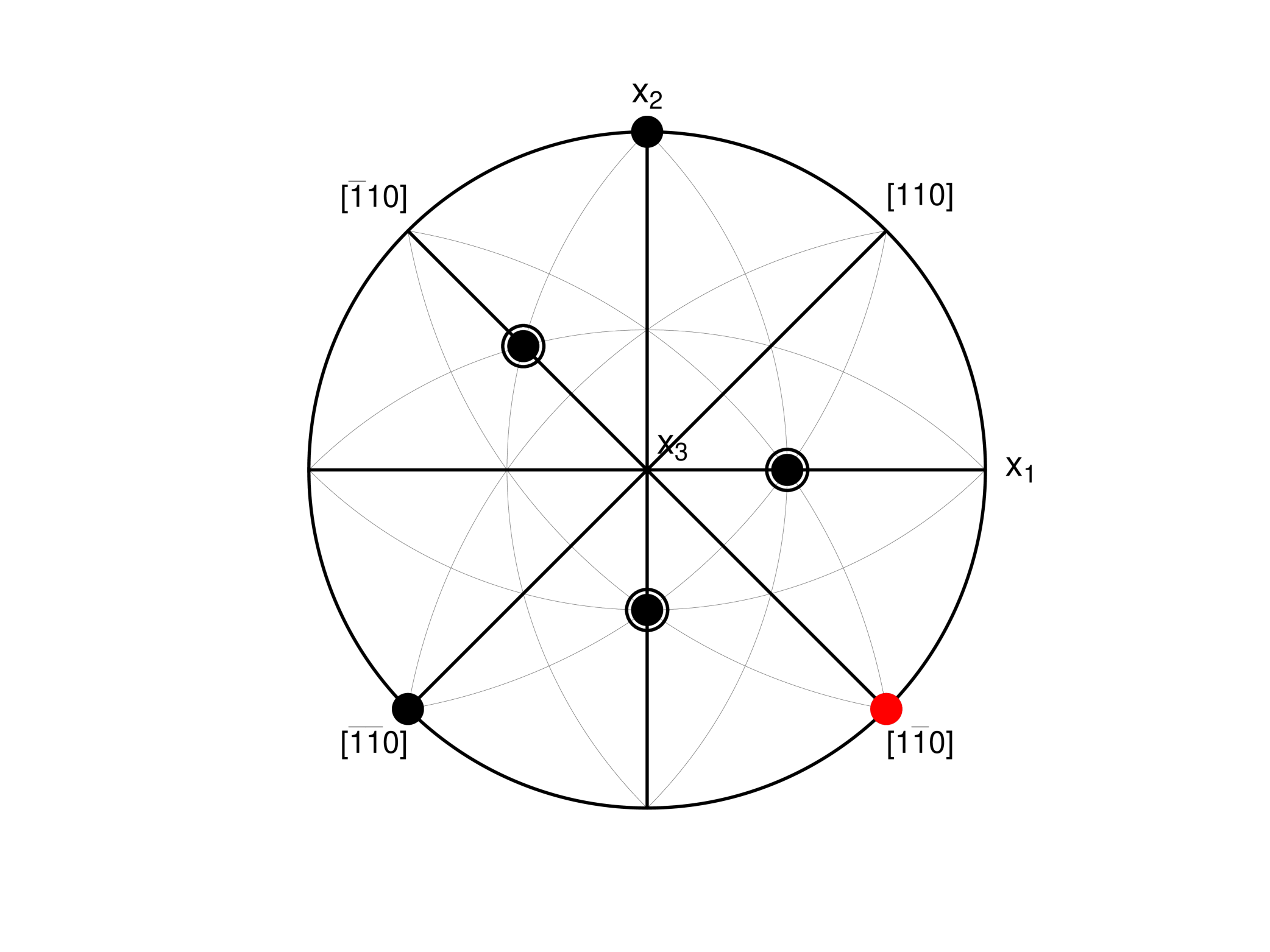
(c) Design 2 Isomorphic to (a)

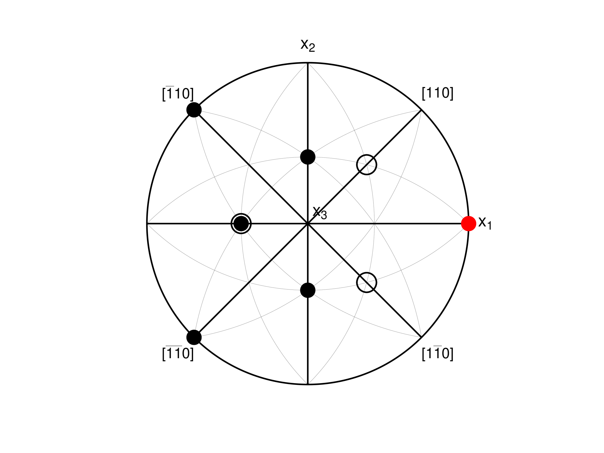
(d) A design not isomorphic to (a)

Figure 4: Stereograms of the spherical components of selected (DP)_S-optimal designs: (a) The design of Gilmour and Trinca (2012), with one point of $B$ occurring once, (b) and (c) designs which exhibit different patterns of points, but which are geometrically isomorphic to (a), and (d) a design, not isomorphic to (a), with one point, $(1,0,0)$, of $B$ occurring once. Points which occurs once are indicated in red.

A cursory examination of the results from the exchange algorithm indicated that designs with one centre point and any one of the nine points in the basis set $B$ occurring once and not twice are (DP)_S-optimal. In terms of geometric isomorphism, consider now a design constructed directly from that of Gilmour and Trinca (2012) but with the the point $(-\frac{1}{\sqrt{2}},0,\frac{1}{\sqrt{2}})$ now replicated twice and the point $(1,0,0)$ occurring once. For clarity, a stereogram of the design is shown in Figure 4(d), with the point occurring once indicated in red. It is clear that the design so constructed is not geometrically isomorphic to the design of Gilmour and Trinca (2012). However, by using arguments based on rotations and reflections, it is straightforward to show that the design represents a class of 24 isomorphic (DP)_S-optimal designs. Furthermore, the same result holds for all designs constructed with one of the points in the set $B$ occurring once. There are therefore nine classes of designs, each comprising 24 geometrically isomorphic designs, and thus a total of $9\times 24=216$ designs. This result is in accord with the fact that $216$ (DP)_S-optimal designs with one centre point were identified from multiple runs of the exchange algorithm.

Consider now the $864$ (DP)_S-optimal designs with two centre points generated from multiple runs of the exchange algorithm. A cursory examination of the results indicated that the points on the sphere of the design comprise two distinct points from the basis set $B$ chosen to occur once and the seven remaining points in $B$ replicated twice. The $\binom{9}{2}=36$ designs so defined were then constructed independently and shown to be (DP)_S-optimal. It now follows from arguments similar to those presented for the (DP)_S-optimal designs with one centre point that each of the designs so constructed represents a class of $24$ geometrically isomorphic designs, thereby yielding $36\times 24=864$ designs which are (DP)_S-optimal and accounting for the designs generated by the exchange algorithm.

4 Discussion

The focus of the present study is on the use of the stereographic projection within the context of experimental design in order to map points on the three-dimensional unit sphere onto the stereogram in two dimensions. The stereogram gives a clear visualisation of the spatial arrangement of the points and can be manipulated in order to emulate rotations of, and reflections about, the main axes. Stereograms for subset designs for the quadratic polynomial model in three independent variables over the unit ball, including the central composite and Box-Behnken designs, are presented in order to fix ideas. An example of the effective use of the stereogram is then introduced and is based on a suite of designs generated numerically by an exchange algorithm. Specifically, it is shown that classes of designs which are geometrically isomorphic can be identified by a judicious choice of operations on the stereogram. More broadly, generating optimal designs by invoking a heuristic invariably yields large numbers of similar designs and the present example reveals how such designs can be inter-related and, thereby, classified.

There are, in fact, many ways of representing an arrangement of points on the three-dimensional sphere in two dimensions, that is on paper, other than the stereogram. Thus, most simply, a drawing of the sphere with the points added or a sketch of the solid with vertices defined by the points can be used but these approaches are tedious to implement and not helpful in comparative studies. Alternatively, since a set of points on the sphere defines a convex polytope, the points can be represented by a 3-vertex-connected planar graph, that is a polyhedral graph, but the sense of the spatial arrangement is then lost. There are, in addition, projections, other than the stereographic projection, such as the orthographic and the gnomonic projections, which can be invoked but these distort the symmetry and, in the latter case, project the points onto an infinite plane tangential to the sphere. On balance therefore, none of the approaches discussed here offers the ease of use, the sense of the spherical space and the flexibility provided by the stereogram, as is required within the context of experimental design.

Finally, it would be remiss not to mention the use of computer-generated three-dimensional models which represent points and solids with vertices on the sphere and which are available in, for example, the programming language Mathematica (2022). Such models can be rotated in space and thereby examined but it is nevertheless not easy to identify the inbuilt symmetry. The question also arises as to whether points on the four-dimensional sphere can be represented as three- or two-dimensional objects. There are ways of doing this, as for example with a Schlegel diagram, but these are complicated to interpret and not immediately useful in design.

References

- Atkinson et al. (2007) Atkinson, A. C., A. N. Donev, and R. D. Tobias (2007). Optimum Experimental Designs, with SAS. Oxford University Press; Oxford.
- Borchardt-Ott (2011) Borchardt-Ott, W. (2011). Crystallography: An Introduction, Third Edition. Springer; Heidelberg.
- Bose and Draper (1959) Bose, R. C. and N. R. Draper (1959). Second order rotatable designs in three dimensions. The Annals of Mathematical Statistics 30, 1097–1112.
- Cheng and Ye (2004) Cheng, S.-W. and K. Q. Ye (2004). Geometric isomorphism and minimum aberration for factorial designs with quantitative factors. The Annals of Statistics 32, 2168–2185.
- De Graef and McHenry (2012) De Graef, M. and M. E. McHenry (2012). Structure of Materials: An Introduction to Crystallography, Diffraction, and Symmetry. Cambridge University Press; Cambridge, UK.
- Dette and Grigoriev (2014) Dette, H. and Y. Grigoriev (2014). -optimal designs for second-order response surface models. The Annals of Statistics 42, 1635–1656.
- gauss (2022) gauss (2022). gauss Programming Language, Release 22.1.0. Aptech Systems, Inc.
- Gilmour (2006) Gilmour, S. G. (2006). Response surface designs for experiments in bioprocessing. Biometrics 62, 323–331.