The Morse-Smale property of the Thurston spine

Abstract.

The Thurston spine consists of the subset of Teichmüller space at which the set of shortest curves, the systoles, cuts the surface into polygons. The systole function is a topological Morse function on Teichmüller space. This paper shows that the Thurston spine satisfies a property defined in terms of the systole function analogous to that of Morse-Smale complexes of (smooth) Morse functions on compact manifolds with boundary.

1. Introduction

The systoles on a closed, connected, orientable hyperbolic surface $S_{g}$ of genus $g$ are the set of shortest geodesics. This is a finite nonempty set that varies with the hyperbolic structure. The Thurston spine is a CW complex contained in $\mathcal{T}_{g}$ consisting of the set of all points at which the set of systoles cut the corresponding surface into polygons. In [16], a construction of a mapping class group-equivariant deformation retraction of $\mathcal{T}_{g}$ onto the Thurston spine, $\mathcal{P}_{g}$ is given. Although Morse theory was not explicitly used, the construction is based on an analogy with the construction of a deformation retraction of a compact manifold with boundary onto the Morse-Smale complex defined by a Morse function.

The purpose of this paper is to relate the structure of $\mathcal{P}_{g}$ to that of the handle decomposition coming from the systole function.

Theorem 1.

Suppose a point $p\in\mathcal{P}_{g}$ has the property that there is a nonempty open cone in $T_{p}\mathcal{T}_{g}$ in which $f_{\mathrm{sys}}$ is increasing. Then (a) the open cone contains a 1-sided limit of tangent vectors to $\mathcal{P}_{g}$. Moreover (b) the set of all such vectors of unit length at $p$ is contractible.

The proofs given in this paper do not assume Thurston’s deformation retraction, and only require Thurston’s Lipschitz map construction from [16], Wolpert’s formula for Dehn twists, convexity, calculus and linear algebra. They will be used to justify part of the construction of [16], and in forthcoming papers to relate geometric, topological, analytic, algebraic and number theoretic properties of Teichmüller space and the mapping class group.

As the systole function is not smooth, there can potentially exist regular points at which there is no open cone of directions in which the systole function is increasing. These points are called boundary points of the systole function. A geometric model for $\mathcal{P}_{g}$ around critical points and boundary points of the systole function is given in Section 5 and an explicit example is worked through.

The Morse theory used in this paper is not the usual (smooth) Morse theory, but the Morse theory of so-called topological Morse functions (defined in Section 2) developed in [13]. It was shown in [1] that the systole function is a topological Morse function. The critical points necessarily occur at points at which the systole function is not smooth. Studying the pieces of the piecewise smooth structure is a key ingredient of most of the proofs in this paper.

Details of the differentiable structure of $\mathcal{P}_{g}$ and what it means to have tangent vectors will be given in Section 2, along with other background and definitions.

Organisation of the paper. In an effort to be self-contained, a fairly detailed section is given, surveying the basic known properties of the objects studied in this paper and introducing the notation and assumptions that will be used. This includes a subsection on Schmutz’s sets of minima; a construction that is perhaps not as well-known in the literature as it deserves to be. In order to understand the properties of the stratification of $\mathcal{T}_{g}$, the topological properties of the “loci” are studied in Section 3. An important concept appears to be that of a balanced locus, which is introduced in Subsection 3.2. More details are given here than is strictly necessary for the proof of the main theorem, as this material appears to be interesting and useful in its own right. Section 4 proves Theorem 1, and similar properties are established for critical and boundary points of $f_{\mathrm{sys}}$ in Section 5.

Acknowledgements

The author would like to thank Stavros Garoufalidis, Olivier Mathieu and Don Zagier for helpful comments.

2. Definitions and conventions

The unique closed topological surface of genus $g$ for $g\geq 2$ will be denoted by $\mathcal{S}_{g}$. When $\mathcal{S}_{g}$ has the additional structure of a marking, i.e. it represents a point of Teichmüller space $\mathcal{T}_{g}$ of $\mathcal{S}_{g}$, it will be denoted by $S_{g}$.

Curves on $\mathcal{S}_{g}$ are nontrivial isotopy classes of embeddings of $S^{1}$ into $S_{g}$, where $S^{1}$ is the unpointed, unoriented 1-sphere. A curve on $S_{g}$ is assumed to inherit a marking, and by abuse of notation, the word curve on $S_{g}$ will often be confused with the image of its unique geodesic representative. The set of curves on $\mathcal{S}_{g}$ will be denoted by $\mathcal{C}_{g}$. A curve will usually be denoted by lowercase $c$ with a subscript, while uppercase $C$ is reserved for finite sets of curves. A geodesic on $S_{g}$ of smallest length will be called a systole. The systole function $f_{\mathrm{sys}}$ is the piecewise-smooth function $\mathcal{T}_{g}\rightarrow\mathbb{R}^{+}$ whose value at a point $x$ is given by the length of the systoles. Throughout the paper it will always be assumed that the elements of a set $C$ of curves have pairwise geometric intersection number at most one, mirroring a property of sets of systoles.

A set of curves on $\mathcal{S}_{g}$ fills the surface if the complement of a set of representatives in minimal position consists of a set of topological disks. The Thurston spine, $\mathcal{P}_{g}$, is therefore the set of all points in $\mathcal{T}_{g}$ at which the systoles fill.

Length functions. Length functions generalise the notion of the length of a curve. A curve $c$ on $\mathcal{S}_{g}$ determines an analytic function $L(c):\mathcal{T}_{g}\rightarrow\mathbb{R}^{+}$ whose value at a point $x$ is equal to the length of the geodesic representative of $c$ at $x$. For an ordered set of curves $C=(c_{1},\ldots,c_{k})$ and a corresponding set of real, positive weights $A=(a_{1},\ldots,a_{k})$, the length function $L(A,C):\mathcal{T}_{g}\rightarrow\mathbb{R}^{+}$ is the analytic function given by

$$L(A,C)(x)\,=\,\sum_{j=1}^{k}a_{j}L(c_{j})(x)$$

When all the weights in $A$ are equal to 1, the map $L(A,C)$ from $\mathcal{T}_{g}$ to $\mathbb{R}^{C}$ will be written $L(C)$ or $L(c)$ when $C=\{c\}$. Length functions are so useful because they satisfy many convexity properties, as shown in [18] for the Weil-Petersson metric, in [9] for earthquake paths and [5] for Fenchel-Nielsen coordinates.

The sublevel set of $L(c)$ is the set of all points of $\mathcal{T}_{g}$ for which $L(c)$ is less than or equal the constant $l\in\mathbb{R}^{+}$, and will be denoted by $L(c)_{\leq l}$. The boundary of $L(c)_{\leq l}$ is then the level set $L(c)^{-1}(l)$. Similarly, the superlevel set $\{x\in\mathcal{T}_{g}\ |\ L(c)(x)\geq l\}$ will be denoted by $L(c)_{\geq l}$.

The lengths of elements of $\mathcal{C}$ is known to satisfy a property that will be referred to as local finiteness. It can be proven from the collar lemma that for any $x\in\mathcal{T}_{g}$, the set of curves of length within $\epsilon$ of $f_{\mathrm{sys}}(x)$ is finite. Consequently, there is a neighbourhood of $x\in\mathcal{T}_{g}$ in which the systoles are contained in the set of curves that are realised as systoles at $x$.

Definition 2 (Systole stratum).

A systole stratum $\mathrm{Sys}(C)$ is the subset of $\mathcal{T}_{g}$ on which $C$ is the set of systoles.

Here the term stratification is used in a minimal sense, following Thurston, to mean a disjoint union of locally closed subsets, for which each point is on the boundary of only finitely many of these locally closed subsets (strata).

The existence of a triangulation of $\mathcal{T}_{g}$ compatible with the stratification follows from [11]. A triangulation of this type is assumed when referring to the boundary of a stratum, or the tangent vector or 1-sided limit of tangent vectors to strata of $\mathcal{P}_{g}$.

At first sight it might seem surprising that $\mathcal{P}_{g}$ is nonempty. This is a consequence of the following proposition, and of the theorem due to Bers’ [4] that $f_{\mathrm{sys}}$ is uniformly bounded from above.

Proposition 3 (Proposition 0.1 of [16], Lemma 4 of [3]).

Let $C$ be a set of curves on $\mathcal{S}_{g}$ that do not fill. Then at any point $p$ of $\mathcal{T}_{g}$, there is an open cone of derivations in $T_{p}\mathcal{T}_{g}$ whose evaluation on every element of {$L(c)\ |\ c\in C\}$ is strictly positive at $p$.

Twist flow. In addition to a length function $L(c)$, a curve $c$ on $\mathcal{S}_{g}$ determines a flow $\mathbb{R}\times\mathcal{T}_{g}\rightarrow\mathcal{T}_{g}$. Choose any set of Fenchel-Nielsen coordinates on $\mathcal{T}_{g}$ defined using a set of curves containing $c$. Then a point $(r,x)$ is mapped to the point in $\mathcal{T}_{g}$ with Fenchel-Nielsen coordinates equal to the coordinates at $x$, except for the twist parameter around $c$, which is incremented by $r$. A flowline will be called a twist path and denoted by $\gamma_{c,x}$, where $x=\gamma_{c,x}(0)$.

This flow will be implicit in most of the arguments in this paper, for the simple reason that for any $c_{1}$ and $c_{2}$ disjoint, $c_{1}$ determines a flow that leaves the level sets of $L(c_{2})$ invariant.

Topological Morse functions. Suppose $M$ is an $n$-dimensional topological manifold. A continuous function $f:M\rightarrow\mathbb{R}^{+}$ will be called a topological Morse function if the points of $M$ are either regular or critical points with respect to $f$. A point $p\in M$ is regular if there is an open neighbourhood $U$ containing $p$, for which $U$ admits a homeomorphic parametrisation by $n$ parameters, one of them being $f$. If $p$ is a critical point there exists a $j\in\mathbb{Z}$, $0\leq j\leq n$, called the index of $p$, and a homeomorphic parametrisation of $U$ by parameters $\{x_{1},\ldots,x_{n}\}$. For every point on $U$

$$f(x)\,-\,f(p)\;=\ \sum_{i=1}^{i=n-j}x_{i}^{2}\,-\,\sum_{i=n-j+1}^{i=n}x_{i}^{2}$$

A reference for topological Morse functions is [13].

Whenever a metric is needed in this paper, the Weil-Petersson metric will be assumed. None of the important concepts are dependent on a specific choice of mapping class group-equivariant metric; in most instances, any other choice would work just as well.

The orthogonal complement of a set of gradients of length functions, $\{\nabla L(c)\ |\ c\in C\}$ will be denoted by $\{\nabla L(c)\ |\ c\in C\}^{\perp}$. Although a metric is needed to define gradients and orthogonal complements, $\{\nabla L(c)\ |\ c\in C\}^{\perp}$ is independent of a choice of metric. This is because it can be defined as a tangent space to the intersection of level sets of length functions.

Tangent cones and cones of increase. There are many places throughout this paper at which objects similar to polyhedra are used. For a polyhedron $P$ in $\mathbb{R}^{d}$, the tangent cone at a point $p\in\partial P$ is the set of $v\in T_{p}\mathbb{R}^{d}$ such that $v=\dot{\gamma}(0)$ for a smooth oriented path $\gamma(t)$ with $\gamma(0)=q$ and $\gamma(\epsilon)$ in $P$ for sufficiently small $\epsilon>0$. For background and definitions relating to polyhedra, see [7] or [2]. When discussing connectivity properties of tangent cones, it is convenient to define the unit tangent cone to be the set of vectors in the tangent cone with unit length, or the $\epsilon$-tangent cone to be the set of all vectors of length $\epsilon$.

As $\mathcal{P}_{g}$ can be triangulated, the tangent cone of $\mathcal{P}_{g}$ and the $\epsilon$-tangent cone at a point $p$ can be defined analogously. When $p$ is on the boundary of more than one simplex, the tangent cone is the union of the tangent cones of the simplices with $p$ on the boundary, similarly for the unit tangent cone and $\epsilon$-tangent cone. Tangent cones of strata are defined analogously. For a triangulation compatible with the stratification, the tangent cone to $\mathrm{Sys}(C)$ at $p$ is the union of the tangent cones of the simplices with interior contained in $\mathrm{Sys}(C)$ with $p$ on the boundary, similarly for the unit tangent cone and $\epsilon$-tangent cone.

Since $f_{\mathrm{sys}}$ is only piecewise smooth, it does not have a gradient at every point. The level set of $f_{\mathrm{sys}}$ is a locally finite intersection of level sets of curves in $\mathcal{T}_{g}$. On a neighbourhood of $x\in\mathcal{T}_{g}$ at which $C$ is the set of systoles, by local finiteness the level set of $f_{sys}$ passing through $x$ lies on the boundary of the intersection $I(C,x)$ of $\{L(c)_{\geq f_{\mathrm{sys}}(x)}\ |\ c\in C\}$. Each of these sublevel sets is linear with respect to some set of Fenchel-Nielsen coordinates, but as the systoles can intersect, $I(C,x)$ is not always an intersection of linear half-spaces. Nevertheless, it is possible to define a tangent cone in the same way as for a polyhedron, and the cone of increase of $f_{\mathrm{sys}}$ at a point $x$ is defined to be the tangent cone of $I(C,x)$.

The cone of increase of $f_{\mathrm{sys}}$ will be called full if it has dimension equal to that of $\mathcal{T}_{g}$, namely $6g-6$. Since $f_{\mathrm{sys}}$ is only a topological, but not smooth, Morse function, it is possible that there exist regular points at which the cone of increase of $f_{\mathrm{sys}}$ is not full. If $p$ is one such point, then $f_{\mathrm{sys}}$ can increase away from $x$ to at most second order. Following Schmutz, these points will be called boundary points of $f_{\mathrm{sys}}$. An alternative definition will be given in Section 2.1, and these points will be studied in Section 5.

A point $y$ on $\partial I(C,x)$ will be called a vertex of $I(C,x)$ if the tangent cone to $I(C,x)$ contains no vector subspaces of $T_{y}\mathcal{T}_{g}$. Otherwise, $p$ will be said to be on a face, where the face corresponds to a maximal vector subspace of the tangent cone of $I(C,x)$ at a point $y\in\partial I(C,x)$, and two such subspaces at points $y_{1}$ and $y_{2}$ determine the same face if $y_{1}$ and $y_{2}$ are connected by a path in $\partial I(C,x)$ along which the vector subspace has fixed dimension and varies smoothly. When the face has codimension 1 in $\mathcal{T}_{g}$, it will be called a facet.

When $I(C,x)$ is replaced by the intersection $D(C,t)$ of sublevel sets $\{L(c)_{\leq t}\ |\ c\in C\}$, tangent cones, facets, faces and vertices are defined analogously.

The fact that $f_{\mathrm{sys}}$ is a topological Morse function, [1], implies that the set of unit tangent vectors in the cone of increase at a regular point of $f_{\mathrm{sys}}$ is contractible, [13].

Stably contractible, stably connected. Tangent cones are first order approximations. In the statement of Theorem 1, when there are strata at $p$ that agree to first order on a subspace of $T_{p}\mathcal{T}_{g}$, in the statement of Theorem 1 and later in the statement of Theorem 22 contractibility or connectivity of the intersection of the cone of increase with the unit tangent cone of $\mathcal{P}_{g}$ at $p$ is not strong enough. A condition ruling out the behaviour shown on the left of Figure 1 is needed.

Figure 1. The Thurston spine near the point $p$ is shown in black, and the boundary of the cone of increase in red. On the left is an example for which the intersection of the cone of increase with the unit tangent cone of $\mathcal{P}_{g}$ at $p$ is neither stably connected nor stably contractible. On the right is an example that is both stably connected and stably contractible.

Let $C$ be the set of systoles at a point $p\in\mathcal{P}_{g}$, and let $I(C,x)\cap\partial B_{\epsilon}(p)$ be the set of all points in $I(C,x)$ at distance $\epsilon$ from $p$. Then the intersection of the cone of increase with the $\epsilon$-tangent cone of $\mathcal{P}_{g}$ at $p$ will be said to be stably contractible or stably connected if the intersection of $I(C,x)\cap\partial B_{\epsilon}(p)$ with $\mathcal{P}_{g}$ is contractible, respectively connected.

Eutactic. In the literature a point $x\in\mathcal{T}_{g}$ in $\mathrm{Sys}(C)$ is defined to be eutactic if for every derivation $v$ in $T_{x}\mathcal{T}_{g}$, either the evaluations $\{vL(c)(x)\ |\ c\in C\}$ are all zero, or there is at least one $c\in C$ for which $vL(c)(x)$ is strictly positive and another for which it is strictly negative. In this paper the term eutactic will be generalised. A set of curves $C$ (not necessarily systoles) will be called eutactic at a point $x$ in $\mathcal{T}_{g}$ if for every derivation $v$ in $T_{x}\mathcal{T}_{g}$, either the evaluations $\{vL(c)(x)\ |\ c\in C\}$ are all zero, or there is at least one $c\in C$ for which $vL(c)(x)$ is strictly positive and another for which it is strictly negative. Similarly, for a fixed subspace $V\in T_{x}\mathcal{T}_{g}$, the set of curves $C$ will be called $V$-eutactic at $x$ if for every derivation $v$ in $V$, either the evaluations $\{vL(c)(x)\ |\ c\in C\}$ are all zero, or there is at least one $c\in C$ for which $vL(c)(x)$ is strictly positive and another for which it is strictly negative.

Thurston’s Lipschitz map construction. A construction of a map $\mathcal{T}_{g}\rightarrow\mathcal{T}_{g}$ will now be surveyed. The input of this construction is $(m,A)$, where $m$ is a geodesic multicurve on $S_{g}$ and $A$ is a set of pairwise disjoint geodesic arcs with endpoints on $m$, meeting $m$ at right angles, and with the property that $A$ has nonzero geometric intersection number with every boundary component of a regular neighbourhood of $m$. The output of the construction is a family of maps $\mathcal{T}_{g}\rightarrow\mathcal{T}_{g}$ which are used to control the change in the lengths of some curves relative to others. This construction was used in [16] to prove Proposition 3, with $m$ isotopic to the boundary of the subsurface filled by $C$, and $A$ a set of arcs that intersect every curve in $C$.

Start with a surface $S_{g}$ representing a point of $\mathcal{T}_{g}$. Cut $S_{g}$ along the geodesic representive of $m$ to get a union of hyperbolic surfaces with boundary. On each boundary component of each of these surfaces, attach a hyperbolic annulus, to obtain a surface without boundary, as shown in Figure 2. Each of the geodesic representatives of arcs in $A$ can be extended to a bi-infinite geodesic in these extended surfaces. Cut the extended surfaces along each bi-infinite geodesic, and glue in a strip of the hyperbolic plane bounded by two infinite geodesics. The widths of the geodesics strips is chosen in such a way that for every curve $c$ in $m$, the curves $c_{1}$ and $c_{2}$ in the extended surfaces corresponding to $c$ have the same length after the strips have been glued in. For each curve $c$ in $m$, cut the extended surfaces along the geodesic representatives of $c_{1}$ and $c_{2}$, and glue the surface together along the resulting boundary components. This gives a new hyperbolic structure. Clearly there are many choices involved in this construction.

In this paper, as in [16], limits are taken as the widths of the strips are allowed to approach zero. The resulting 1-parameter families of maps do not change the length of any curve disjoint from the geodesic representatives of the elements of $m$ and $A$, and lengthen $m$ and any curve with geodesic representative disjoint from $m$ that intersects one or more of the arcs in $A$.

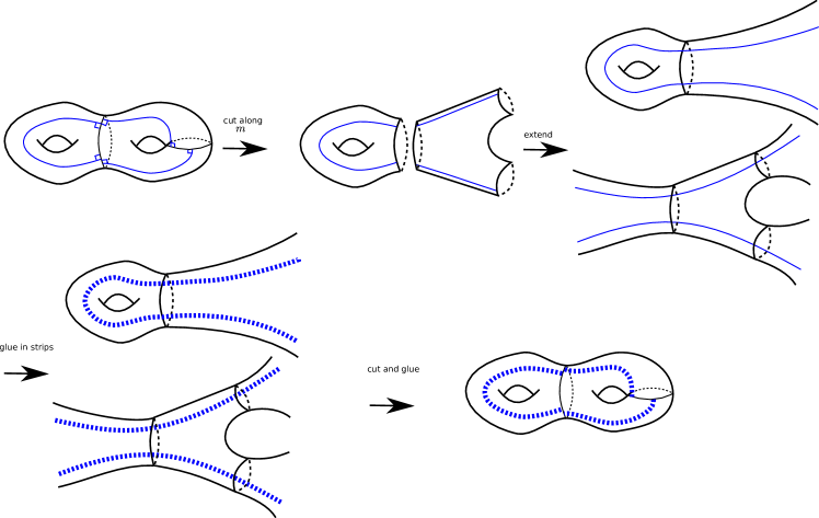
Figure 2. Thurston’s Lipschitz map construction, where $m$ is shown in black and $A$ in blue in the upper leftmost figure.

2.1. Sets of Minima

As an attempt at parameterising $\mathcal{T}_{g}$ without reference to punctures or marked points, Schmutz introducted the concept of cell decompositions of Teichmüller space parametrised by length functions. Schmutz’s construction will be surveyed here as it provides insight into the differential topology $\mathcal{T}_{g}$.

A length function $L(A,C)$ with fixed $A\in\mathbb{R}_{+}^{|C|}$ is convex with respect to the Weil-Petersson metric[18]. A necessary and sufficient condition for $x$ to represent the minimum of $L(A,C)$ in $\mathcal{T}_{g}$ is therefore that the gradient of $L(A,C)$ is zero at $x$. When $C$ is eutactic at $x$ there exists an $A$ for which the unique minimum of $L(A,C)$ occurs at $x$. If the curves in $C$ do not fill, Proposition 3 ensures that $L(A,C)$ has no minimum in the interior of $\mathcal{T}_{g}$.

Definition 4 ($\mathrm{Min}(C)$).

The subset $\mathrm{Min}(C)$ of $\mathcal{T}_{g}$ is the set of all points at which $L(A,C)$ has a minimum for some $A$ with strictly positive entries. Alternatively, $\mathrm{Min}(C)$ is the set of all $x\in\mathcal{T}_{g}$ at which $C$ is eutactic.

There is a notion of closure of $\mathrm{Min}(C)$ that will be denoted by $\overline{\mathrm{Min}(C)}$.

Definition 5 (Modified version of Proposition 2 of [15]).

Let $C$ be a finite set of closed geodesics that fills $S_{g}$. A point $p$ of $\mathcal{T}_{g}$ is in $\overline{\mathrm{Min}(C)}$ iff there does not exist a derivation in $T_{p}\mathcal{T}_{g}$ whose evaluation on each length function of a curve in $C$ is strictly positive. Then $\partial\mathrm{Min}(C)$ is defined to be the set of points in $\overline{\mathrm{Min}(C)}{\smallsetminus}\mathrm{Min}(C)$

Lemma 6 (Lemma 14 of [14]).

Any point $x\in\mathcal{T}_{g}$ in $\partial\mathrm{Min}(C)$ is in $\mathrm{Min}(C_{i})$, for some filling $C_{i}\subsetneq C$

Lemma 1 of [14] showed that when $C$ fills, any choice of $A$ with strictly positive entries determines a length function $L(A,C)$ with a minimum realised somewhere in $\mathcal{T}_{g}$. It therefore follows from Proposition 3 that $\mathrm{Min}(C)$ is nonempty iff $C$ is a filling set of curves. There exists therefore a surjective map $\phi_{C}:\mathbb{R}^{|C|}_{+}\twoheadrightarrow\mathrm{Min}(C)$, where $\phi(A)$ is the point in $\mathrm{Min}(C)$ at which $L(A,C)$ has its minimum. Since $\phi_{C}$ is not injective, the entries of the $k$-tuple $A$ are parameters, not coordinates. For $C=\{c_{1},\ldots,c_{k}\}$, let $F(C):\mathcal{T}_{g}\rightarrow\mathbb{R}^{k}_{+}$ be the differentiable function $x\mapsto\bigl{(}L(c_{1}),\ldots,L(c_{k})\bigr{)}$. When the rank of $F(C)$ is constant on $\mathrm{Min}(C)$, $\mathrm{Min}(C)$ is a cell, otherwise it is “pinched” at places where the rank drops.

Boundary points of the systole function. It was shown in [1] that a critical point of $f_{\mathrm{sys}}$ occurs exactly where $\mathrm{Sys}(C)$ intersects $\mathrm{Min}(C)$. Schmutz defined a boundary point of $f_{\mathrm{sys}}$ to be a point at which $\mathrm{Sys}(C)$ intersects $\partial\mathrm{Min}(C)$. By Lemma 6 this is a point at which $\mathrm{Sys}(C)$ intersects $\mathrm{Min}(C^{\prime})$, for $C^{\prime}\subsetneq C$. There are reasons for calling such points boundary points of $f_{\mathrm{sys}}$, but boundary points of $f_{sys}$ should not be confused with the usual topological notion of boundary. The structure of critical and boundary points of $f_{\mathrm{sys}}$ will be discussed in Section 5. By Corollary 22 and Theorem 23 of [14], critical points and boundary points of $f_{\mathrm{sys}}$ are isolated, so there are only finitely many of them modulo the action of the mapping class group.

3. Minimal sets of filling curves

Suppose $C$ is a set of filling curves on $S_{g}$, any two of which intersect in at most one point. The set $C$ will be called a minimal set of filling curves if no proper subset of $C$ fills. This section begins by proving some key lemmas about minimal sets of filling curves, and ends by discussing a property that generalises many of the important properties of minimal sets of filling curves.

A basic property of minimal sets of filling curves is the following, which will be assumed from now on without comment.

Lemma 7.

Suppose $C$ is a minimal set of filling curves. For any curve $c\in C$, there is a curve $c^{*}$ that intersects $c$ but does not intersect any of the other curves in $C$.

Proof.

Suppose every curve on $\mathcal{S}_{g}$ that intersects $c\in C$ also intersects a curve in $C{\smallsetminus}\{c\}$. Then $C{\smallsetminus}\{c\}$ fills, contradicting the assumption that $C$ is a minimal filling set. ∎

3.1. Key Lemmas

This subsection proves some key lemmas about minimal sets of filling curves and their loci, which will now be defined.

Definition 8 (Locus $E(C)$ labelled by $C$).

The locus of points in $\mathcal{T}_{g}$ at which the lengths of all curves in $C$ are equal will be denoted by $E(C)$, and called the locus labelled by $C$. Alternatively,

(1) $$E(C)=\{x\in\mathcal{T}_{g}\ |\ L(c)(x)=L(c^{\prime})(x)\ \forall c,c^{\prime}\in C\}$$

The set $E(C)$ is called a locus to emphasise the similarity with the locus of points equidistant from a finite set of points $\{p_{1},\ldots,p_{k}\}$ in $\mathbb{R}^{n}$. The analogy is drawn by replacing the set of points in $\mathbb{R}^{n}$ by points in the completion of $\mathcal{T}_{g}$ with respect to the Weil-Petersson metric, where $p_{i}$ for $i=1,\ldots,k$ is a point at which the curve $c_{i}\in C$ has been pinched. Note that by convexity, $L(c_{i})$ increases monotonically with Weil-Petersson distance from $p_{i}$. Note that $\mathrm{Sys}(C)\subsetneq E(C)$.

Recall that $\mathcal{C}$ is the set of curves on $\mathcal{S}_{g}$. Denote by $F(\mathcal{C})$ the map from $\mathcal{T}_{g}$ to $\mathbb{R}^{\mathcal{C}}$ taking $x$ to the collection of lengths $\{L(c)(x)\ |\ c\in\mathcal{C}\}$, and by $\overline{F}(\mathcal{C}):\mathcal{T}_{g}\rightarrow\mathbb{R}^{\mathcal{C}}/\mathbb{R}$ the composition of this map with the projection from $\mathbb{R}^{\mathcal{C}}$ (arbitrary maps from $\mathcal{C}$ to $\mathbb{R}$) to its quotient by $\mathbb{R}$ (the constant maps). Fix $C$ and $d\in\mathbb{R}^{\mathcal{C}}/\mathbb{R}$. Then $E(C,d)$ is defined to be the set of points in $\mathcal{T}_{g}$ for which the lengths of the curves in $C$ realise the specified differences in $d|_{C}$, in other words

(2) $$E(C,d)=\{x\in\mathcal{T}_{g}\ |\ L(c)(x)+d(c)=L(c^{\prime})(x)+d(c^{\prime})\ \forall c,c^{\prime}\in C\}$$

When every element of $d|_{C}$ is zero, $d$ will be omitted.

The next lemma will be used in proving results about loci of minimal sets of filling curves.

Lemma 9.

For a set $C$ of filling curves, suppose $c\in C$ has the property that $C{\smallsetminus}\{c\}$ is not filling. Then for any point $x$ in $\mathcal{T}_{g}$ there is a nonempty open cone of directions in $T_{x}\mathcal{T}_{g}$ with the property that each derivation $v$ in the cone is strictly negative when evaluated on $L(c)$ and strictly positive when evaluated on the length of any curve in $C{\smallsetminus}\{c\}$.

Definition 10 ($C$-generic).

Suppose $C$ is a (not necessarily proper) subset of a minimal set of filling curves. A point $x\in\mathcal{T}_{g}$ is $C$-generic if for every $c\in C$, the sum of the cosines of the angles of intersection of $c$ with $c^{*}$ is nonzero, for some choice of $c^{*}$.

Proof.

Wolpert’s twist formula states that the rate of change of the length of $L(c)$ with respect to the twist parameter around $c^{*}$ is equal to the sum of the cosines of the angles of intersection of $c$ with $c^{*}$. For points of $\mathcal{T}_{g}$ that are $\{c\}$-generic, the lemma follows from Wolpert’s twist formula, [17], and Proposition 3. For points that are not $\{c\}$-generic, the proof uses Thurston’s Lipschitz map construction from Section 2. The geodesic multicurve $m$ is given by $c^{*}$, and it will now be explained how to obtain the set of arcs $A$.

If $c$ intersects $c^{*}$ just once, and the cosine of the Weil-Petersson angle of intersection is zero, then $c\cap(S_{g}{\smallsetminus}c^{*})$ is an arc with endpoints on $c^{*}$ making angle $\pi/2$ with $c^{*}$. Choose this arc to be an element of $A$ and add more arcs to the set, subject to the constraints in the definition of $A$, until each curve in the set $C{\smallsetminus}\{c\}$ intersects at least one arc in $A$. This choice of $m$ and $A$ then determines family of maps, taking an infinitesimal element of this family gives a vector corresponding to a derivation that is strictly negative when evaluated on $L(c)$ and strictly positive when evaluated on the length of any curve in $C{\smallsetminus}\{c\}$.

When $c$ intersects $c^{*}$ more than once, the condition that the cosines of the angles of intersection are equal to zero guarantees the existence of at least two arcs $\{e_{1},\ldots,e_{k}\}$ of $c^{*}\cap(S_{g}{\smallsetminus}c)$ with the property that the signs of the cosines of the angles at the endpoints are different.

A set of cycles $A_{i}:=\{a_{1}^{\prime},\ldots,a_{m}^{\prime}\}$ is obtained, consisting of the connected components of the boundary of a normal neighbourhood of the union of the geodesics $c$ and $c^{*}$. By choosing $c^{*}$ to have the smallest possible geometric intersection number with $c$, it is possible to assume without loss of generality that each element of $A_{i}$ is homotopically nontrivial. This is because the curves in the set $C$ intersect pairwise at most once, and $c$ is the only curve in $C$ to intersect $c^{*}$. A curve in $C{\smallsetminus}\{c\}$ that intersects a homotopically nontrivial element $a_{k}^{\prime}$ of $A_{i}$ must intersect $c$ at least twice, which is not possible. When $a_{k}^{\prime}$ is homotopically trivial, the curve $c^{*}$ can then be replaced by a homotopically nontrivial connected component of the boundary of a normal neighbourhood of $c^{*}\cup a_{k}^{\prime}$ that intersects $c$.

Each cycle in $A_{i}$ has edges alternating between edges lying along $c$ and $c^{*}$. From each cycle $a_{l}^{\prime}$, remove a single edge lying along $c^{*}$ to obtain an arc $a_{l}$ with endpoints on $c^{*}$. Whenever possible, the arc removed should have the property that the angles at the vertices of the cycle $a_{l}^{\prime}$ at the endpoints of the edge, to the same side of the cycle, are both less than or equal to $\pi/2$. At least one of the edges $e_{i}$ in the set $\{e_{1},\ldots,e_{k}\}$ has this property. An arc $a_{l}$ obtained by deleting $e_{i}$ will be called central.

A central arc has the property that the shortest representative of its homotopy class with endpoints on $c^{*}$ is disjoint from the geodesic representative of $c$. There exist central arcs intersecting each connected component of the boundary of a normal neighbourhood of $c^{*}$. Choose a set $A$ of pairwise disjoint arcs as above, containing $\{a_{1},\ldots,a_{m}\}$. Then a map constructed from this choice of $m$ and $A$, for which the widths of the central arcs are sufficiently large relative to the widths of the other arcs, gives a vector corresponding to a derivation that is strictly negative when evaluated on $L(c)$ and strictly positive when evaluated on the length of any curve in $C{\smallsetminus}\{c\}$. ∎

Given a set $C$ of curves, a point $x\in\mathcal{T}_{g}$ will be called a minimum of $C$ if $L(C)|_{E(C,d(x))}$ has a minimum at $x$. Here $d(x)$ is the value of $d$ for which $E(C,d(x))$ passes through $x$.

Lemma 11.

Let $C$ be a minimal set of filling curves. Then the gradients of the lengths of the curves in $C$ are linearly independent everywhere in $\mathcal{T}_{g}$ away from minima of $C$.

Remark 12.

Note that this lemma also holds for subsets of minimal sets of filling curves.

Proof.

As in the proof of Lemma 9, there are two cases. When $x$ is $C$-generic, the lemma follows from Wolpert’s twist formula. To prove the lemma for $C$-nongeneric points that are not minima of $C$, it will be shown that $C$-generic points satisfy a geometric property that implies linear independence of the gradients. It will then be shown that Lemma 9 implies this property can only break down on open sets. As the set of $C$-nongeneric points are not open, the lemma then follows.

Let $L(C,t,d):=\{x\in\mathcal{T}_{g}\ |\ L(c)(x)=t+d(c)\ \forall\ c\in C\}$ be a level set of $E(C,d)$ from Equation (2) on which the length of each $c\in C$ is given by $t+d(c)$. Then $D(C,t,d)$ is defined to be the intersection of the sublevel sets $\{L(c)_{\leq t+d(c)}\ |\ c\in C\}$. Recall the definition of faces, facets and tangent cones from Section 2. Since each sublevel set is strictly convex with respect to, for example, the Weil-Petersson metric, [18], the intersection $D(C,t,d)$ is convex, in particular connected. Each facet of $D(C,t,d)$ is contained in a level set $L(c)^{-1}(t+d(c))$ for some $c\in C$. Lower dimensional faces of $D(C,t,d)$ are intersections of level sets.

The assumption that $E(C)$ is nonempty guarantees that for sufficiently large $t$ the intersection $L(C,t)=\{x\in\mathcal{T}_{g}\ |\ L(c)(x)=t\ \forall\ c\in C\}$ will be nonempty, and is then the lowest dimensional face of $D(C,t)$.

Let $\{x_{1},\ldots,x_{n}\}$ be a standard set of coordinates on $\mathbb{R}^{n}$, and denote by

(3) $$\mathbb{H}^{n}=\{(x_{1},\ldots,x_{n})\in\mathbb{R}^{n}\ |\ x_{1}x_{2}\ldots x_{n}=0\}\subset\mathbb{R}^{n}$$

a union of hyperplanes passing through the origin of $\mathbb{R}^{n}$. Then the level sets of $\{L(c)\ |\ c\in\leavevmode\nobreak\ C\}$ will be said to have the $\mathbb{H}$-property at $x\in\mathcal{T}_{g}$ if $T_{x}\mathcal{T}_{g}\simeq\mathbb{R}^{6g-6}$ has a basis $\{\frac{\partial}{\partial x_{1}},\ldots,\frac{\partial}{\partial x_{n}}\}$ that includes $\{\nabla L(c)\ |\ c\in C\}$. In particular, when the level sets of $\{L(c)\ |\ c\in C\}$ have the $\mathbb{H}$-property, the following conditions are satisfied:

1. Each $C^{\prime}\subset C$ determines exactly one face of $D(C,t,d)$ adjacent to $p$ contained in a level set of $E(C^{\prime},t,d)$. This will be called the face labelled by $C^{\prime}$.

2. The face from part 1 labelled by $C^{\prime}$ has connected unit tangent cone

3. The tangent cone at $p$ of the face labelled by $C^{\prime}\subset C$ has codimension equal to $|C^{\prime}|-1$.

A tangent cone of a face of $D(C,t,d)$ labelled by $C^{\prime}$ will be called full if it has codimension $|C^{\prime}|-1$, which is the codimension of $E(C^{\prime})$ when the lengths of curves in $C^{\prime}$ have linearly independent gradients. Similarly, a tangent cone to $D(C,t,d)$ is full if it has dimension equal to the dimension of $\mathcal{T}_{g}$.

Claim: At a $C$-generic point, the level sets of $\{L(c)\ |\ c\in C\}$ have the $\mathbb{H}$-property.

The claim will be proven using twist paths. For each $c\in C$, at $p$, both $D(C{\smallsetminus}\{c\},t,d)$ and $L(C{\smallsetminus}\{c\},t,d)\cap\partial D(C{\smallsetminus}\{c\},t,d)$ have a product structure. One term of the product (called an $\mathbb{R}$-factor below) is diffeomorphic to $\mathbb{R}$, and corresponds to the parameter on the $c^{*}$-twist paths. The intersection of $L(c)^{-1}(t+d(c))$ with $L(C{\smallsetminus}\{c\},t,d)\cap\partial D(C{\smallsetminus}\{c\},t,d)$ cuts through this $\mathbb{R}$ factor; on one side, $c$ is longer than the other curves in $C$ and on the other it is shorter. The existence of an $\mathbb{R}$-factor corresponding to $c\in C$ guarantees the existence of a face labelled by $C{\smallsetminus}\{c\}$; the face is the union of subintervals of $\gamma_{c^{*},y}$ with $y\in L(C,t,d)\cap\partial D(C,t,d)$ on which $L(c)+d(c)<L(c_{i})+d(c_{i})$ for all $c_{i}\in C{\smallsetminus}\{c\}$. The $C$-generic assumption guarantees this is not empty, because there is a direction along $\gamma_{c^{*},y}$ for $y\in L(C,t,d)\cap\partial D(C,t,d)$ in which $L(c)$ is decreasing and the lengths of the other curves in $C$ are stationary. For $c_{i}$ and $c_{j}\in C$, the face labelled by $C{\smallsetminus}\{c_{i},c_{j}\}$ lies between the faces labelled by $C{\smallsetminus}\{c_{i}\}$ and $C{\smallsetminus}\{c_{j}\}$. Faces labelled by smaller subsets are constructed similarly. Connectivity of unit tangent cones to faces is a consequence of linear independence, as is fullness of the tangent cones. This concludes the proof of the claim.

At all $C$-generic points that are not minima of $C$, the dimension of the tangent cone to the face labelled by $C^{\prime}\subset C$ remains constant. This is a consequence of linear independence of $\{\nabla L(c)\ |\ c\in C\}$ at $C$-generic points.

The assumption that $p$ is $C$-generic will now be dropped. Suppose $p$ is a point of $L(C,t,d)$ on $\partial D(C,t,d)$ that is not a minimum. This assumption ensures that $t$ can be decreased slightly and the connected component of $L(C,t,d)\cap\partial D(C,t,d)$ containing $p$ does not disappear.

When $C$ does not fill, Proposition 3 implies that at $p$, the tangent cone to $D(C,t,d)$ is full; these are directions in which the lengths of all the curves in $C$ are decreasing. When $C$ fills, by assumption $p$ is not a critical point or boundary point of $f_{\mathrm{sys}}$, hence by Definition 5 the tangent cone to $D(C,t,d)$ is also full. For any $p\in L(C,t,d)\cap\partial D(C,t,d)$ and any $c\in C$, Lemma 9 gives a full tangent cone of the intersection of $D(C{\smallsetminus}\{c\},t,d)$ and $L(c)_{\geq t+d(c)}$. This is the cone of directions in which $L(c)$ is increasing and the curves in $C{\smallsetminus}\{c\}$ are decreasing. As the tangent cones at $p$ of $D(C,t,d)$ and the intersection of $D(C{\smallsetminus}\{c\},t,d)$ and $L(c)_{\geq t+d(c)}$ are full for every $c\in C$, and by convexity the unit tangent cone of $D(C{\smallsetminus}\{c\},t,d)$ is connected for every $c\in C$, each $c\in C$ determines a facet of $D(C,t,d)$ with $p$ on the boundary.

If the level sets $\{L(c)\ |\ c\in C\}$ have the $\mathbb{H}$-property at $p\in\mathcal{T}_{g}$, this implies that the vectors $\{\nabla L(c)(p)\ |\ c\in C\}$ are linearly independent. Note that the converse is not true. One example is given by the gradients in $\mathbb{R}^{4}$ of the functions

$$f_{1}=e^{x_{1}}+e^{-x_{2}}\ \ \ f_{2}=e^{x_{2}}+e^{-x_{3}}\ \ \ f_{3}=e^{-x_{3}}+e^{x_{4}}\ \ \ f_{4}=e^{-x_{4}}+e^{x_{1}}$$

In this example, the gradients are linearly independent, except where $x_{2}=x_{4}$. Moreover, this set of functions has the property that at every point there is an open cone of directions in which all four functions are increasing, and for each $f_{i}$, $i=1,\ldots,4$, there is an open cone of directions in which $f_{i}$ is decreasing and the other functions increasing. Define $D(p)$ to be the intersection of the sublevel sets $\{f_{i}(x)\leq f_{i}(p)\ |\ i=1,2,3,4\}$. As for $D(C,t,d)$, there is a facet of $D(p)$ along a level set of each of the functions. This means that when $x_{2}=x_{4}$ at $p$, $\partial D(p)$ has no face determined by $\{f_{1},f_{2}\}$; the tangent space at $p$ to the submanifold on which $f_{1}=f_{2}$ consists of directions in which one of $\{f_{3},f_{4}\}$ is increasing, and the other decreasing. Similarly for $f_{3}$ and $f_{4}$. On a neighbourhood of the submanifold on which $x_{2}=x_{4}$, the level sets also cannot have the $\mathbb{H}$-property.

As in the example, away from minima, Lemma 9 and Proposition 3 imply that if the level sets of $\{L(c)\ |\ c\in C\}$ do not have the $\mathbb{H}$-property at $p$, this is also the case on a neighbourhood of $p$. However, the $C$-nongeneric points are a set of measure zero, and the level sets of $\{L(c)\ |\ c\in C\}$ have the $\mathbb{H}$-property at $C$-generic points. This concludes the proof of the theorem. ∎

Lemma 13.

Let $C$ be a minimal set of filling curves and $C^{\prime}\subset C$. The only minima of $C^{\prime}$ and $C$ occur in the intersection of $E(C,d)$ with $\mathrm{Min}(C)$.

Proof.

It was shown in the proof of Lemma 11 that for $c\in C$ there are no saddle points of $L(c)|_{L(C{\smallsetminus}\{c\},t,d)}$ and for $c\in C^{\prime}$ there are no saddle points of $L(c)|_{L(C^{\prime}{\smallsetminus}\{c\},t,d)}$. It follows that each connected component of $E(C,d)$ and each connected component of $E(C^{\prime},d)$ has at most one minimum of the restriction of the lengths of curves in $C$ respectively $C^{\prime}$. By Lemma 11 the gradients of the lengths of curves in $C$ respectively $C^{\prime}$ are linearly independent everywhere away from this minimum.

Every point $x$ in $\mathcal{T}_{g}$ is in $E(C,d)$ for some $d(x)$. It will now be shown that any $E(C,d)$ intersects $\mathrm{Min}(C)$ in a unique point.

That $E(C,d)$ intersects $\mathrm{Min}(C)$ in at most one point is an immediate consequence of the definition of $\mathrm{Min}(C)$. If $E(C,d)$ intersected $\mathrm{Min}(C)$ in two points, $p_{1}$ and $p_{2}$, then either the lengths of the curves at both points are equal, or the lengths of the curves at one of the points, call it $p_{1}$, are smaller. In the first case, there are length functions with minima realised at both points, contradicting convexity. In the second case, a contradiction is obtained, because the length function with global minimum at $p_{2}$ is smaller at $p_{1}$.

On a connected component of $E(C,d)$ that intersects $\mathrm{Min}(C)$, the gradients of the lengths of curves are linearly independent away from $\mathrm{Min}(C)$. Since $C=\{c_{1},\ldots,c_{k}\}$ is a minimal set of filling curves, it follows from Lemma 5 of [14] that $\bigl{\{}\nabla L(c_{2})-\nabla L(c_{1}),\ldots,\nabla L(c_{k})-\nabla L(c_{1})\bigr{\}}$ are linearly independent everywhere on $\mathrm{Min}(C)$. Repeated applications of the pre-image lemma (see, for example, Corollary 5.14 of [10]) then implies that each $E(C,d)$ passing through $\mathrm{Min}(C)$ is an embedded submanifold.

Since $C$ is a minimal set of filling curves, by Lemma 9 and Theorem 10 of [14], $\mathrm{Min}(C)$ is a continuously differentiable cell with empty boundary. Since each $E(C,d)$ intersects $\mathrm{Min}(C)$ in at most one point, there is a differentiable bijection from $\mathrm{Min}(C)$ to a subset of elements of $\mathbb{R}_{+}^{|C|}$ whose entries sum to zero; a point $x\in\mathrm{Min}(C)$ is mapped to the tuple $d$ for which $E(C,d)$ passes through $x$.

Claim: The set of loci $E(C,d)$ that intersect $\mathrm{Min}(C)$ with varying $d$ foliate $\mathcal{T}_{g}$.

To prove the claim, let $\{x_{i}\}$ be a sequence of points in $\mathcal{T}_{g}$ converging to a point $x$ on $E(C,d)$. Suppose that the points of the sequence are sufficiently close to $\mathrm{Min}(C)$ such that each $x_{i}$ is in an $E(C,d(x_{i}))$ that intersects $\mathrm{Min}(C)$. Since $d$ varies smoothly over $\mathcal{T}_{g}$, $d(x_{i})$ approaches $d(x)$. Suppose also that $E(C,d(x))$ intersects $\mathrm{Min}(C)$.

If the claim were not true, it would be possible to choose a sequence $\{y_{i}\}$, with each $y_{i}$ in the same connected component of $E(C,d(x_{i}))$ as the point $x_{i}$, such that $y$ is in a connected component of $E(C,d(y))$ disjoint from $\mathrm{Min}(C)$. Moreover, it is possible to choose the sequences in such a way that each $x_{i}$ and $y_{i}$ are arbitrarily close together. This then contradicts the fact that $E(C,d(x)=d(y))$ is an embedded submanifold. The claim then follows by contradiction. This concludes the proof of the lemma in the case of filling curves.

For a nonfilling subset $C^{\prime}$ of $C$, any minima of the lengths of the curves in $C^{\prime}$ restricted to $E(C^{\prime},d)$ must occur within $\mathrm{Min}(C)$; otherwise this would give a minimum on some $E(C,d)$ away from $\mathrm{Min}(C)$. However, by Lemma 5 of [14], the assumption that $C$ is a minimal set of filling curves implies that the gradients of the lengths of curves in $C^{\prime}$ are everywhere linearly independent on $\mathrm{Min}(C)$. This rules out the existence of minima on $E(C^{\prime},d)$, as these can only occur at a point at which $L(c)^{-1}(t+d(c))$ intersects $L(C^{\prime}{\smallsetminus}\{c\},t,d)$ nontransversely for any $c\in C^{\prime}$. ∎

Corollary 14.

Let $C$ be a minimal set of filling curves. When $E(C)$ is nonempty, it is a connected, embedded submanifold of $\mathcal{T}_{g}$. The restriction to $E(C)$ of the lengths of the curves in $C$ is strictly convex and has a unique minimum.

Proof.

In the proof of Lemma 13 it was shown that $E(C)$ is an embedded submanifold. Moreover, it was shown that on each connected component of $E(C)$, the only nonregular point of the restriction of the lengths of curves in $C$ is a unique minimum where the connected component passes through $\mathrm{Min}(C)$ and that $E(C)$ can intersect $\mathrm{Min}(C)$ at most once. This proves convexity and connectivity.
∎

3.2. Balanced loci

This subsection discusses a property of loci. This concept is related to the way loci of filling curves intersect corresponding sets of minima, leading to a trichotomy of three fundamentally different types of loci.

Suppose now that $C$ is any finite set of curves on $\mathcal{S}_{g}$ that intersect pairwise at most once. It follows from Lojasiewicz’s theorem, [11] that $E(C,d)$ admits a triangulation, i.e. it is a simplicial complex. Consequently, $E(C,d)$ from Equation (2) has a dimension, and in the interior of each simplex, it has a tangent space.

Definition 15 ($E(C,d)$ is balanced at $x$).

Let $x$ be a point of $E(C,d)$ contained in the interior of a locally top dimensional simplex. Then $E(C,d)$ will be said to be balanced at $x$ if $x$ is in $\mathrm{Min}(C)$ or there is a vector $v_{C}$ in $T_{x}E(C,d)$ in the interior of the convex hull of $\{\nabla L(c)\ |\ c\in C\}$.

Away from critical points of $f_{\mathrm{sys}}$, an alternative definition is that $E(C,d)$ is balanced at $x$ if there is a codimension 1 subspace $V$ of $T_{x}\mathcal{T}_{g}$ with the property that $C$ is $V$- eutactic. It follows from the second definition that the property of being balanced is independent of the choice of metric.

Remark 16.

When $C$ is a minimal set of filling curves, it was shown in Corollary 14 that $E(C,d)\subset\mathcal{T}_{g}$ is an embedded submanifold, in which case it has a tangent space at every point. The statement that $E(C,d)$ is balanced at every point therefore makes sense.

When $E(C,d)$ is balanced at a point $x$, then for any choice of metric, the orthogonal complement of $v_{C}$ consists of vectors $\{\nabla L(c)\ |\ c\in C\}^{\perp}$, or directions in which the length of at least one curve in $C$ is strictly decreasing, and the length of at least one other curve is strictly increasing.

Remark 17.

When $E(C,d)$ is balanced at $x$ and $x$ is not a critical point, this implies that there is a direction $v_{C}$ in $T_{q}E(C,d)$ in which the lengths of the curves in $C=\{c_{1},\ldots,c_{k}\}$ are increasing. While it is possible that $a_{1}L(c_{1})+\ldots+a_{k}L(c_{k})$ could be a direction in which some of the lengths of curves in $C$ are decreasing, when such a vector is tangent to $E(C,d)$, the constraints defining $E(C,d)$ force this to be a direction in which the lengths of all the curves in $C$ are increasing.

Proposition 18.

Let $C$ be a subset (not necesssarily proper) of a minimal set of filling curves. Then $E(C,d)$ is balanced at every point.

Proof.

The proof is essentially an application of Lagrange multipliers. Fix $C=\{c_{1},\ldots,c_{k}\}$ and suppose to begin with that $C$ is a minimal set of filling curves. Denote by $v_{C}$ the common gradient of the restrictions of $\{L(c_{1}),\ldots,L(c_{k})\}$ to $E(C,d)$. When $E(C,d)$ is balanced at $x$, it is possible to find a $k$-tuple $(a_{1},\ldots,a_{k})$ in $\mathbb{R}_{+}^{k}$, with entries normalised to sum to one, and such that $v_{C}=a_{1}\nabla L(c_{1})+\ldots+a_{k}\nabla L(c_{k})$ in $T_{x}\mathcal{T}_{g}$.

Claim: For $x\in E(C,d){\smallsetminus}\mathrm{Min}(C)$ at which $E(C,d)$ is balanced, $(a_{1},\ldots,a_{k})$ are the parameters of the point in $\mathrm{Min}(C)$ through which the locus $E(C,d)$ passes. Recall that such a point was shown to be unique.

To prove the claim, recall that on every $E(C,d)$, by Corollary 14, there is a unique point $p(C,d)$ in the intersection $E(C,d)\cap\mathrm{Min}(C)$; the point $p(C,d)$ is the point at which the restrictions to $E(C,d)$ of the lengths of curves in $C$ have their minimum. Define

$$L(t):=\cup_{d}\{y\in E(C,d)\ |\ L(c)(y)=L(c)\left(p(C,d)\right)+t\ \forall\ c\in C\}$$

Choose $t$ so that the connected component of $L(t)$ passes through the point $x$. It follows from Theorem 10 of [14] that $\mathrm{Min}(C)$ is a $C^{1}$-submanifold, hence so is $L(t)$.

Recall that the entries of the tuple $(a_{1},\ldots,a_{k})$ are normalised to sum to one. By construction, $x$ is a local minimum of the length function $a_{1}L(c_{1})+\ldots+a_{k}L(c_{k})$ along any path in $L(t)$ crossing $E(C,d(x))$ transversely. It follows from the method of Lagrange multipliers that $a_{1}\nabla L(c_{1})+\ldots+a_{k}\nabla L(c_{k})$ is normal to $L(t)$ everywhere in the intersection $E(C,d(x))\cap L(t)$, and hence parallel to the normal vector field $\frac{\partial}{\partial t}$ on $L(t)$. In $E(C,d(x))$, the common gradient of the length functions, $v_{C}$, is also always orthogonal to the level sets of the lengths of curves in $C$. This proves the claim.

As this construction works for any value of $t>0$, it follows that the $k$-tuple $d(x)$ defining the locus $E(C,d(x))$ passing through $x$ is the value of $d(C)$ for which $E(C,d(x))$ passes through the point in $\mathrm{Min}(C)$ representing the minimum of the length function $a_{1}L(c_{1})+\ldots+a_{k}L(c_{k})$, and $v_{C}$ is parallel to $a_{1}\nabla L(c_{1})+\ldots+a_{k}\nabla L(c_{k})$ everywhere on $E\big{(}C,d(x)\big{)}$. This concludes the proof in the case of $C$ filling.

For $C^{\prime}\subsetneq C$, $E(C^{\prime},d)$ is a union $\cup_{d\in D}E(C,d)$ where $D$ is the set of tuples with the property that every entry corresponding to a curve in $C^{\prime}$ is equal. Suppose $k=|C^{\prime}|$. The condition that $C$ is minimal set of filling curves ensures that the map $\phi$ defined in Section 2.1 from normalised $|C|$-tuples in $\mathbb{R}^{|C|}_{+}$ to points of $\mathrm{Min}(C)$ is a bijection. Since $\phi$ is also $C^{1}$ in this case by Theorem 10 of [14], it follows that for every point on $E(C^{\prime},d)$, there is a 1-parameter family of nearby loci into which a given entry of the $k$-tuple $d(C^{\prime})$ is increasing and one or more other entries are decreasing. This is a direction in which the length of some curves in $C^{\prime}$ are increasing and others decreasing. ∎

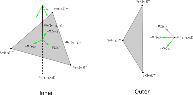
Figure 3. Inner versus outer loci. In the figure on the right, the locus should be regarded as coming out of the page. A filling set of curves that intersect pairwise at most once must have cardinality at least four. This figure represents a lower dimensional analogue, where $\mathrm{sys}(\{c_{i})^{\infty}$ denotes a point in the completion of $\mathcal{T}_{g}$ with respect to the Weil-Petersson metric at which the curve $c_{i}$ has been pinched.

Once again allowing $C$ to be any set of curves that intersects pairwise at most once, now that $\mathrm{Min}(C)$ can have a boundary, a new phenomenon occurs.

Inner, outer and borderline loci. A connected component of $E(C,d)$ is

• inner if it passes through a point of $\mathrm{Min}(C)$,

• borderline if it passes through a point of $\partial\mathrm{Min}(C)$,

• outer if it is disjoint from $\overline{\mathrm{Min}(C)}$.

Lower dimensional analogues of inner and outer loci are shown in Figure 3.

An inner locus $E(C,d)$ has the property that at the global minimum point of the lengths of curves in $C$ restricted to $E(C,d)$, there is no direction in which all the lengths of all the curves in $C$ are decreasing, whereas there is an open cone of such directions at the minimum point when $E(C,d)$ is outer.

Observe that the set $C$ of curves defining an outer or borderline locus strictly contain a minimal set of filling curves, because otherwise, by Lemma 6, $\mathrm{Min}(C)$ would have empty boundary. Similarly, if $\mathrm{Sys}(C)$ is not balanced at some point $x$, then by Proposition 18, $C$ strictly contains a minimal set of filling curves.

4. Proof of the Morse-Smale Property

This section proves the following reworded version of Theorem 1 from the Introduction.

Theorem 19.

Suppose a point $p\in\mathcal{P}_{g}$ has the property that the cone of increase of $f_{\mathrm{sys}}$ at $p$ is full. Then the intersection of this cone of increase with the $\epsilon$-tangent cone of $\mathcal{P}_{g}$ is (a) nonempty and (b) stably contractible for sufficiently small $\epsilon>0$.

Before beginning the proof of the theorem, a lemma will be proven. This lemma is probably well-known, but as the author could not give a reference, a proof will be given here. It is not essential to the proof of Thoerem 1, but helps to motivate the construction.

Lemma 20.

Fix $C$ and $l\in\mathbb{R}^{+}$. The set

$$L(C,l):=\{x\in\mathcal{T}_{g}\ |\ L(c)(x)=l\ \forall\ c\in C\}$$

is compact iff the curves in $C$ fill $\mathcal{S}_{g}$.

Proof.

If $C$ is a filling set, compactness of the level set is a consequence of Lemma 1 of [14], convexity of length functions and closure of level sets. When the geodesics in $C$ do not fill, there is a curve $c^{*}$ disjoint from all the geodesics in $C$. The set $L(C,l)$ is invariant under the flow $\mathbb{R}\times\mathcal{T}_{g}\rightarrow\mathcal{T}_{g}$ obtained by changing the twist parameter around $c^{*}$ and therefore noncompact. ∎

The proof of Theorem 1 will now be given.

Proof of theorem 1 from the Introduction.

Fix a point $p\in\mathrm{Sys}(C)\subset\mathcal{P}_{g}$ with a full cone of increase of $f_{\mathrm{sys}}$. Part (a) of the theorem will first be proven by showing the existence of a stratum of $\mathcal{P}_{g}$ above $p$. By above $p$ is meant, a stratum containing a sequence $\{x_{i}\}$ of points converging to $p$ such that $f_{\mathrm{sys}}(x_{i})>f_{\mathrm{sys}}(p)$. Similarly, a level set of $f_{\mathrm{sys}}$ is above $p$ if the value of $f_{\mathrm{sys}}$ on this level set is larger than $f_{\mathrm{sys}}(p)$. The adjective below will be used similarly.

Suppose there is a nonzero vector $v_{C}$ in $T_{p}\mathcal{T}_{g}$ tangent to $E(C)$ giving a direction in which the lengths of curves in $C$ are all increasing at the same rate. In this case, part (a) of the theorem follows immediately; by local finiteness there is a stratum $\mathrm{Sys}(C)$ above $p$. It is therefore possible to assume without loss of generality that even when there is a nonzero vector $v_{C}\in T_{p}\mathcal{T}_{g}$, it is not tangent to $E(C)$ because equality of curve lengths only holds to first order in the direction of $v_{C}$.

Recall from Section 2 that for $x\in\mathcal{T}_{g}$, $I(C,x):=\{y\in\mathcal{T}_{g}\ |\ L(c)(y)\geq f_{\mathrm{sys}}(x)\ \forall c\in C\}$. The set $D(C,x):=\{y\in\mathcal{T}_{g}\ |\ L(c)(y)\leq f_{\mathrm{sys}}(x)\ \forall c\in C\}$ is defined similarly. Since $D(C,x)$ is an intersection of convex sets, it is also convex. It follows that the unit tangent cone to $D(C,x)$ at $x$ is connected. As this is the same up to sign as the unit tangent cone to $I(C,x)$ at $x$, the latter is also connected.

As a result of local finiteness, in a neighbourhood of $p$, the level set of $f_{\mathrm{sys}}$ passing through $p$ is the boundary of $I(C,p)$. Recall that the tangent cone to $I(C,p)$ at $p$ is the cone of increase of $f_{sys}$ at $p$. By continuity of $f_{\mathrm{sys}}$, the level sets of $f_{\mathrm{sys}}$ passing through points close to $p$ converge to the level set passing through $p$.

Throughout this proof, $x\in\mathcal{T}_{g}$ will denote a point with $f_{\mathrm{sys}}(x)>f_{\mathrm{sys}}(p)$ in a neighbourhood of $p$ sufficiently small such that the systoles are contained in the set $C$.

A face (or subdivided face) of $I(C,x)$ or $I(C,p)$ will be said to be labelled by a subset $C^{\prime}$ of $C$, if the face is contained in the intersection of level sets of curves in $C^{\prime}$, and $C^{\prime}$ is not contained in a larger subset of $C$ for which this holds. For varying $x$, a face of $I(C,x)$ labelled by $C^{\prime}\subset C$ gives a 1-parameter family of faces contained in a stratum $\mathrm{Sys}(C^{\prime})$ above $p$. The stratum $\mathrm{Sys}(C^{\prime})$ will be said to be traced out by the 1-parameter family of faces of $I(C,x)$ labelled by $C^{\prime}$. Note that $f_{\mathrm{sys}}$ is smooth when restricted to a stratum, so a level set of $f_{\mathrm{sys}}$ restricted to the interior of a stratum of $\mathcal{P}_{g}$ cannot contain more than one adjacent face of $I(C,x)$.

Claim: In a sufficiently small neighbourhood of $p$, there is a stratum of $\mathcal{P}_{g}$ traced out by the 1-parameter family either of a locally lowest dimensional face of the level sets above $p$ or a subdivision of such a face.

This claim implies part (a) of the theorem.

To prove the claim, the first step is to understand the geometric, topological and combinatorial structure of $I(C_{m},x)$, where $C_{m}$ is a minimal set of filling curves contained in $C$. The point $p$ cannot be a minimum of $C_{m}$; if it were, by Lemma 13 it would be in the intersection of $\mathrm{Sys}(C)$ with $\mathrm{Min}(C_{m})$, in which case it would be either a boundary point of $f_{\mathrm{sys}}$, or a critical point of $f_{\mathrm{sys}}$ by [1], contradicting the assumption that the tangent cone of $f_{\mathrm{sys}}$ is full at $p$. Moreover, as critical points and boundary points of $f_{\mathrm{sys}}$ are isolated, there are no critical points or boundary points of $f_{\mathrm{sys}}$ on a neighbourhood of $p$. Consequently, by Lemma 11, on a sufficiently small neighbourhood of $p$, the level sets $\{L(c)^{-1}(t)\ |\ c\in C_{m}\}$ have the $\mathbb{H}$-property, and the gradients of the lengths of curves in $C_{m}$ are linearly independent. It is therefore possible to choose $x$ to be in $E(C_{m})$, in which case $I(C_{m},x)=\{y\in\mathcal{T}_{g}\ |\ L(c)(y)\geq L(c)(x)\ \forall c\in C_{m}\}$.

Recall the definition of the twist flow from Section 2. Denote by $c^{*}$ a curve with nonzero geometric intersection number with $c\in C_{m}$ that is disjoint from any curve in $C_{m}{\smallsetminus}\{c\}$. Then a flowline through $x$ will be denoted by $\gamma_{c^{*},x}$.

The lowest dimensional face of the boundary of $I(C_{m},p)$ is the level set of $E(C_{m})$ containing $p$. This is a topological sphere by Corollary 14. All other faces of $I(C_{m},p)$ are noncompact, and contained in level sets of loci labelled by nonfilling subsets of $C_{m}$. The same is true for $I(C_{m},x)$. Recall that Lemma 20 states that a level set of $E(C^{\prime})$ is compact iff $C^{\prime}$ fills.

Define a function $f_{sys}^{C}:\mathcal{T}_{g}\rightarrow\mathbb{R}$ for which $f_{sys}^{C}(y)=\min\{L(c)(y)\ |\ c\in C\}$.

If $x$ is a $C_{m}$-generic point on a level set of $E(C_{m})$ on $\partial I(C_{m},x)$, then $\partial I(C_{m},x)$ contains a ray along $\gamma_{c^{*},x}$ emanating from $x$ for any $c\in C_{m}$. This ray is contained in the intersection of a level set of $E(C_{m}{\smallsetminus}\{c\})$ with $\partial I(C_{m},x)$. A point $x$ at which the path $\gamma_{c^{*},x}$ leaves $\partial I(C_{m},x)$ is necessarily a point in a level set labelled by a set of curves containing $c$. This is a crucial statement to understand. At such a point $x$, $\gamma_{c^{*},x}$ leaves the level set of $f_{sys}^{C}$ given by $\partial I(C_{m},x)$. This means there is a direction along $\gamma_{c^{*},x}$ at $x$ at which $f_{sys}^{C}$ is changing along $\gamma_{c^{*},x}$, and hence there is a curve in $C$ intersecting $c^{*}$ that is equal shortest at $x$. Moreover, the direction in which $f_{sys}^{C}$ is changing along $\gamma_{c^{*},x}$ is a direction in which $f_{sys}^{C}$ is decreasing along $\gamma_{c^{*},x}$. The function $f_{sys}^{C}$ cannot be increasing along $\gamma_{c^{*},x}$ in this direction, because $x$ is in a face labelled by a set of curves, not all of which intersect $c^{*}$. The lengths of the curves disjoint from $c^{*}$ do not change along $\gamma_{c^{*},x}$.

For $C_{m}$-nongeneric $x$, $\partial I(C_{m},x)$ contains the entire path $\gamma_{c^{*},x}$. In the left hand side of Figure 4, $x_{1}$ is $C_{m}$-generic, and $x_{2}$ is not. The right hand side of Figure 4 shows a lower dimensional analogue of the faces of $I(C_{m},x)$ and the twist paths they contain, with the directions corresponding to $\{\nabla L(c)\ |\ c\in C_{m}\}^{\perp}$ suppressed. As explained in Section 2, the subspace $\{\nabla L(c)(x)\ |\ c\in C_{m}\}^{\perp}$ of $T_{x}\mathcal{T}_{g}$ is independent of the choice of metric, and is the tangent space to the lowest dimensional face of $I(C_{m},x)$ at $x$, shown as the blue circle in the figure.

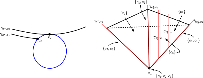
Figure 4. On the left, the lowest dimensional face of $I(C_{m},x)$ is a level set of $\mathrm{Sys}(C_{m})$ and shown in blue. The point $x_{1}$ is a $C_{m}$-generic point, and $x_{2}$ is not. On the right is a cross section of $I(C_{m},x_{1})$ in the fictitious case with $|C_{m}|=3$ with the tangent space to the blue circle on the left suppressed. The point $x_{1}$ on the right corresponds to the point $x_{1}$ shown on the left.

The claim clearly follows in the case $C_{m}=C$, as level sets of $f_{\mathrm{sys}}$ above $p$ lie on $\partial I(C_{m},x)$ on a neighbourhood of $p$, and the lowest dimensional face of $\partial I(C_{m},x)$ lies along a level set of $E(C_{m})$. By local finiteness, this 1-parameter family of lowest dimensional faces then traces out the stratum $\mathrm{Sys}(C_{m})$ above $p$, as required.

The case $C\neq C_{m}$ will now be discussed. Starting with $C_{m}$, one curve will be added at a time, until $C$ is reached.

For small $\epsilon>0$, choose $x(\epsilon)$ in the level set of $f_{\mathrm{sys}}(p)+\epsilon$.

It will first be ruled out that for some $c_{i}\in C_{m}$, $L(c)^{-1}(f_{\mathrm{sys}}(p)+\epsilon)$ intersects $\partial I(C_{m},x(\epsilon))$ along an entire twist path $\gamma_{c_{i}^{*},x^{\prime}}$ parallel to a path through a $C_{m}$-nongeneric point on the compact face of $\partial I(C_{m},x(\epsilon))$, in such a way that the compact face of $I(C_{m},x(\epsilon))$ is contained in the interior of the sublevel set $L(c)_{\leq f_{\mathrm{sys}}(p)+\epsilon}$. This would give an $I(C_{m}\cup\{c\},x(\epsilon))$ foliated by $c_{i}^{*}$ twist paths, on which none of the shortest curves in the set $C_{m}\cup\{c\}$ intersect $c_{i}^{*}$. This contradicts Lemma 9. As it was shown that the set of unit length vectors pointing into $I(C_{m},x(\epsilon))$ is connected, Lemma 9 and the intermediate value theorem together imply the existence of a face of $I(C_{m}\cup\{c\},p)$ along a level set of $L(c_{i})$, and hence a face of $I(C_{m}\cup\{c\},x(\epsilon))$ along a level set of $L(c_{i})$.

Suppose now that $L(c)^{-1}(f_{\mathrm{sys}}(p)+\epsilon)$ intersects a face of $I(C_{m},x(\epsilon))$ labelled by a set of curves $C^{\prime\prime}\subset(C_{m}{\smallsetminus}\{c_{i}\})$. Then $L(c)^{-1}(f_{\mathrm{sys}}(p)+\epsilon)$ intersects some rays $\gamma_{c_{i}^{*},y}$ for varying $y$ that foliate this face. These rays have endpoints in a face labelled by a subset $C^{\prime}$ of $C$ containing $c_{i}$. If none of the curves $C^{\prime\prime}\cup\{c\}$ intersect $c_{i}$, the rays along $\gamma_{c_{i}^{*},y}$ must also be contained in $L(c)^{-1}(f_{\mathrm{sys}}(p)+\epsilon)$, so $L(c)^{-1}(f_{\mathrm{sys}}(p)+\epsilon)$ also intersects the face of $I(C_{m},x(\epsilon))$ labelled by $C^{\prime}$.

When the intersection of $L(c)^{-1}(f_{\mathrm{sys}}(p)+\epsilon)$ is with a twist path $\gamma_{c_{i}^{*},y}$ passing through a $C_{m}$-nongeneric point of the compact face of $I\left(C_{m},x(\epsilon)\right)$, the intersection of this compact face with $L(c)^{-1}(f_{\mathrm{sys}}(p)+\epsilon)$ might not be transverse, so the subset of $\partial I(C_{m}\cup\{c\},x(\epsilon))$ labelled by the largest set of curves will not be a face, but a subdivided face.

It has now been shown that $\partial I(C_{m}\cup\{c\},x(\epsilon))$ has a lowest dimensional face, or a subdivided face, labelled by a set of filling curves. This proves the claim in the case $C=C_{m}\cup\{c\}$. When $C_{m}\cup\{c\}\subsetneq C$, taking intersections with level sets of subsequent curves in $C$, this argument can be repeated, with the only difference being that a ray along $\gamma_{c_{i}^{*},y}$ might be replaced by a compact interval $e_{i}(y)$ contained in $\gamma_{c_{i}^{*},y}$, with endpoints on faces labelled by sets of curves that intersect $c_{i}^{*}$. This concludes the proof of the claim, and hence of part (a) of the theorem.

Part b. The proof of part (b) begins by showing stable connectivity of the intersection of the cone of increase of $f_{\mathrm{sys}}$ at $p$ with the $\epsilon$-tangent cone of $\mathcal{P}_{g}$ at $p$. The proof of connectivity is based on the following construction, which will be referred to as the “wedge argument”. The wedge argument will first be explained, and then it will be related to stable connectivity of the intersection of the cone of increase of $f_{\mathrm{sys}}$ at $p$ with the $\epsilon$-tangent cone of $\mathcal{P}_{g}$ at $p$.

The wedge argument is based on the following: Suppose $C_{1}\subsetneq C$ and $C_{2}\subsetneq C$ are labels of faces of $I(C,x(\epsilon))$, both of which are on the boundary of a face of $I(C,x(\epsilon))$ labelled by $C_{1,2}\subsetneq C$. As $\epsilon$ approaches zero, the 1-parameter families of faces labelled by $C_{1},C_{1,2}$ and $C_{2}$ trace out a “wedge” with apex on $p$, as shown in Figure 5. A 1-parameter family of faces labelled by $C_{1,2}$ will be described as collapsing faces or collapsing onto $C$.

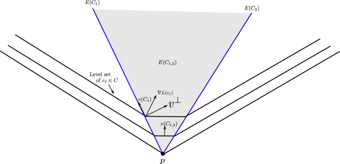
Figure 5. Obtaining the contradiction in the proof of part (b) of Theorem 1 involves showing that the collapsing faces making up the “wedge” (grey) between $E(C_{1})$ and $E(C_{2})$ prevent $E(C_{1})$ and $E(C_{2})$ from both being balanced.

The loci traced out by the 1-parameter families of faces of $I\left(C,x(\epsilon)\right)$ as labelled by $C_{1},C_{1,2}$ and $C_{2}$ have the property that the lengths of curves in $C_{1}{\smallsetminus}C_{1,2}$ are increasing into the level sets of $E(C_{1,2})$ (i.e. faces of $I(C,x(\epsilon))$ labelled by $C_{1,2}$) in the wedge, and similarly, the lengths of curves in $C_{2}{\smallsetminus}C_{1,2}$ are increasing into the level sets of $E(C_{1,2})$ in the wedge. This is not a property satisfied by any loci intersecting at $p$, but uses the assumption that the loci are traced out by faces on the boundary of $I\left(C,x(\epsilon)\right)$ for varying $\epsilon$.

Denote by $v_{C_{1}}$ the gradient of the restriction to $E(C_{1})$ of the lengths of the curves in $C_{1}$, similarly for $v_{C_{1,2}}$.

The existence of the wedge ensures that $E(C_{1})$ and $E(C_{2})$ cannot both be balanced at every point within a neighbourhood of $p$. This can be seen as follows: For at least one of $E(C_{1})$ and $E(C_{2})$, without loss of generality this can be assumed to be $E(C_{1})$, there is a direction orthogonal to $v_{C_{1}}$ in which the lengths of curves in $C_{1}$ are all increasing. This is the direction indicated as $v^{\perp}$ in Figure 5. The vector $v_{C_{1}}$ is not in the convex hull of $\nabla L(c_{1})$ and $v_{C_{1,2}}$, where $c_{1}$ as shown in Figure 5 is a curve in $C_{1}{\smallsetminus}C_{1,2}$.

For the wedge argument, it is not necessary that the faces of $I\left(C,x(\epsilon)\right)$ labelled by $C_{1}$ and $C_{2}$ are on the boundary of the same face labelled by $C_{1,2}$; there may be more than one face between the faces labelled by $C_{1}$ and $C_{2}$ tracing out the wedge, as shown on the left in Figure 6. Here it is used that $I\left(C,x(\epsilon)\right)$ is the intersection of super level sets, so large interior solid angles, such as in the right side of Figure 6, are not possible.

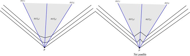
Figure 6. On the left, a wedge traced out by two faces of $I\left(C,x(\epsilon)\right)$. The definition of $I\left(C,x(\epsilon)\right)$ as the intersection of super level sets rules out the “nonconvex” configuration on the right.

It will now be explained how the wedge argument shows stable connectivity of the intersection of the cone of increase of $f_{\mathrm{sys}}$ at $p$ with the $\epsilon$-tangent cone of $\mathcal{P}_{g}$ at $p$. It is essentially always the case that locally top dimensional strata in $\mathcal{P}_{g}$ are balanced. If $\mathrm{Sys}(C_{1})$ and $\mathrm{Sys}(C_{2})$ were locally top dimensional balanced strata in $\mathcal{P}_{g}$, traced out by 1-parameter families of faces of $I\left(C,x(\epsilon)\right)$, that determine different connected components of the cone of increase of $f_{\mathrm{sys}}$ at $p$ with the $\epsilon$-tangent cone of $\mathcal{P}_{g}$ at $p$, then the wedge argument would give a contradiction.

Denote by $C_{1,2}^{1}$ the set of nonfilling curves labelling the stratum in the wedge next to $\mathrm{Sys}(C_{1})$, as shown in Figure 6. Similarly for $C_{1,2}^{2}$.

In the unlikely case that a locally top dimensional stratum is not balanced everywhere in the intersection with a neighbourhood of $p$, a similar proof by contradiction is obtained by projecting to a vector subspace of the tangent space of $\mathcal{T}_{g}$. For a point $y\in E(C_{1})\cap I\left(C,x(\epsilon)\right)$, this vector space is spanned by $v_{C_{1}}$ and the tangent space to a twist path in $E(C_{1,2}^{1})\cap I(C,x(\epsilon))$, as will now be explained.

Since $C_{1}$ and $C_{2}$ fill and $C_{1,2}^{1}$ and $C_{1,2}^{2}$ do not, it will be shown that it is possible to assume without loss of generality that there is a curve $c_{1}\in C_{1}{\smallsetminus}C_{1,2}^{1}$ with the property that $C_{1}{\smallsetminus}\{c_{1}\}$ is not filling, and $\mathrm{Sys}(C_{2})$ is either balanced in the intersection with a neighbourhood of $p$ or there is a curve $c_{2}\in C_{2}{\smallsetminus}C_{1,2}^{2}$ with the property that $C_{2}{\smallsetminus}\{c_{2}\}$ is not filling. Let $c_{1}^{*}$ be a curve intersecting $c_{1}$ and disjoint from all the curves in $C_{1}{\smallsetminus}\{c_{1}\}$. Then by local finiteness, $\mathrm{Sys}(C_{1,2}^{1})$ is foliated by twist paths around $c_{1}^{*}$, into which $L(c_{1})$ is increasing away from $\mathrm{Sys}(C_{1})$.

A contradiction is obtained as follows: if $\mathrm{Sys}(C_{2})$ is balanced in a neighbourhood of $p$, then at any point $y\in E(C_{1})\cap I\left(C,x(\epsilon)\right)$ in a sufficiently small neighbourhood of $p$, the tangent vector $\dot{\gamma}_{c_{1}^{*},y}$ to the twist path $\gamma_{c_{1}^{*},y}$ pointing into $E(C_{1,2}^{1})\cap I\left(C,x(\epsilon)\right)$ makes an angle of more than $\pi/2$ with $v_{C_{1}}$, and is in the boundary of the cone of increase of $f_{\mathrm{sys}}$ at $y$. Let $C_{m}\subset C_{1}$ be a subset of a minimal set of filling curves. Then the assumption that $C_{1}{\smallsetminus}\{c_{1}\}$ is nonfilling implies that$v_{C_{1}}(y)-v_{C_{m}}(y)$ is contained in the orthogonal complement of $\dot{\gamma}_{c_{1}^{*},y}$. This implies that there is a face of $I(C_{m},y)$ that makes an interior angle of more than $\pi/2$ with $v_{C_{m}}(y)$, which is a contradiction to the model for $I(C_{m},y)$ discussed at the beginning of this proof. When $E(C_{2})\cap I\left(C,x(\epsilon)\right)$ is not balanced, by relabelling $C_{1}$ and $C_{2}$ if necessary, once again at a point $y\in E(C_{1})\cap I\left(C,x(\epsilon)\right)$, the tangent vector $\dot{\gamma}_{c_{1}^{*},y}$ pointing into $E(C_{1,2}^{1})\cap I\left(C,x(\epsilon)\right)$ makes an angle of more than $\pi/2$ with $v_{C_{1}}$, giving a contradiction.

It will now be explained how it is possible to assume without loss of generality that $C_{1}{\smallsetminus}\{c_{1}\}$ is not filling and $C_{2}{\smallsetminus}\{c_{2}\}$ is not filling. There are two observations needed here. Firstly, in the wedge argument, it is possible to replace $C$ with a subset $C^{\prime}$ to obtain the contradiction. Secondly, it is not needed that $C_{1}$ and $C_{2}$ fill, only that $C_{1}$ fills a larger subsurface than $C_{1,2}^{1}$, and similarly for $C_{2}$ and $C_{1,2}^{2}$. If there is no $c_{1}\in C$ and $c_{2}\in C_{2}$ satisfying the assumption, it is therefore possible to apply the wedge argument with $C$ replaced by a subset $C^{\prime}$ for which the assumption holds. When deleting curves from $C$, note that the wedge structure is preserved by the fact that the length of every curve in $C_{1}$ intersecting $c_{1}^{*}$ is increasing (at least to second order) away from $E(C_{1})$ into the twist path $\gamma_{c_{1}^{*},y}$ in $E(C_{1,2}^{1})\cap I(C^{\prime},x)$ contained in the wedge. This is because $f_{\mathrm{sys}}$ would otherwise be decreasing away from the face of $I(C,x)$ labelled by $C_{1}$ into the face of $I(C,x)$ labelled by $C_{1,2}^{1}$, which is impossible because these faces are contained in the same level set.

This concludes the proof of stable connectivity of the intersection of the cone of increase of $f_{\mathrm{sys}}$ at $p$ with the $\epsilon$-tangent cone of $\mathcal{P}_{g}$ at $p$.

For a minimal set of filling curves $C_{m}\subset C$, the argument will now proceed by starting with the simplest nontrivial case $C_{m}\cup\{c\}$ and adding curves in $C{\smallsetminus}C_{m}$ one at a time until the entire set $C$ is reached. The final step is to show that for $C_{m}\subset C^{\prime}\subsetneq C$, taking an intersection of the superlevel set $L(c)_{\geq f_{\mathrm{sys}}(p)+\epsilon}$ with $I\left(C^{\prime},x(\epsilon)\right)$ does not destroy stable contractibility by creating holes amongst the faces of $I(C^{\prime},x(\epsilon))$ labelled by sets of filling curves. Since the diameter of any holes approach zero as $\epsilon$ approaches zero, it is possible to adapt the wedge argument to obtain a contradiction to the existence of a hole. However, as it is also possible to provide a more illustrative argument giving an explicit model showing how any holes that are created are filled by other strata in $\mathcal{P}_{g}$, this will now be presented. For ease of notation, holes created within an individual stratum will be considered; the construction for holes intersecting more than one stratum is analogous.

Definition 21 (Dependent curves).

A set $C$ of curves are dependent at $x\in\mathcal{T}_{g}$ if the set of gradients of their lengths are linearly dependent.

When $C_{m}\cup\{c\}$ are not dependent at $p$, this holds on a neighbourhood of $p$, so the level set $L(c)^{-1}(f_{\mathrm{sys}}(p)+\epsilon)$ intersects the faces of $I\left(C_{m},x(\epsilon)\right)$ transversely for sufficiently small $\epsilon$. The set of vectors in $T_{p}E(C_{m})$ giving directions in which the lengths of curves in $C_{m}$ are increasing, but no faster than the length of $L(c)$, is the solution to a linear equation. It follows that intersecting $L(c)^{-1}_{\geq(f_{\mathrm{sys}}(p)+\epsilon)}$ with $I(C_{m},x(\epsilon))$ does not create holes in the level sets of $E(C_{m})$ on $\partial I\left(C_{m},x(\epsilon)\right)$.

When $C_{m}\cup\{c\}$ are dependent at $p$, a hole in the level sets of $E(C_{m})$ on $\partial I\left(C_{m},x(\epsilon)\right)$ can only arise if $L(c)$ has a local minimum on the level sets of $E(C_{m})$ above $p$, as shown in Figure 7 (a).

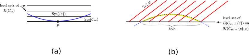
Figure 7. Part (a) shows the level sets of $E(C_{m})$ above $p$ when the restriction of $L(c)$ to the level sets of $E(C_{m})$ has a local minimum above $p$. $\mathrm{Sys}(C_{m}\cup\{c\})$ is shown in blue. Part (b) shows a level set of $E(C_{m})$ on $\partial I(C_{m},x(\epsilon))$. In the case shown in Part (a), $I(C_{m}\cup\{c\},x(\epsilon))$ is obtained from $I(C_{m},x(\epsilon))$ by intersecting with $L(c)_{\geq f_{\mathrm{sys}}(p)+\epsilon}$, the boundary of which is shown by a blue dotted line on the right. The red lines are rays along $\gamma_{c_{i}^{*},y}$ contained in a face of $I(C_{m},x(\epsilon))$ labelled by $C_{m}{\smallsetminus}\{c_{i}\}$. The hole in $E(C_{m})$ is filled by the yellow highlighted ball $\mathcal{B}(\{c\}\cup C_{m}{\smallsetminus}\{c_{i}\})$.

Claim: when the restriction of $L(c)$ to the level sets of $E(C_{m})$ has a local minimum above $p$, for sufficiently small $\epsilon$, there is a ball $\mathcal{B}(\{c\}\cup C_{m}{\smallsetminus}\{c_{i}\})$ on $\partial I(C_{m}\cup\{c\},x(\epsilon))$ such that

• $\mathcal{B}(\{c\}\cup C_{m}{\smallsetminus}\{c_{i}\})$ is the intersection of $L(c)^{-1}(f_{\mathrm{sys}}(p)+\epsilon)$ with a face of $I(C_{m},x(\epsilon))$ labelled by $C_{m}{\smallsetminus}\{c_{i}\}$ for some $c_{i}\in C_{m}$

• $\{c\}\cup C_{m}{\smallsetminus}\{c_{i}\}$ is a filling set of curves

• $\mathcal{B}(\{c\}\cup C_{m}{\smallsetminus}\{c_{i}\})$ fills the hole in the level set of $E(C_{m})$ on $\partial I(C_{m}\cup\{c\},x(\epsilon))$.

The claim follows from convexity of $L(c)$ with respect to the Weil-Petersson metric. As a result of this convexity, the tangent plane to the level set $L(c)^{-1}(f_{\mathrm{sys}}(p)+\epsilon)$ must be contained in $L(c)_{\geq f_{\mathrm{sys}}(p)+\epsilon}$ at every point. At any point $y_{\mathrm{hole}}$ on $\partial I\left(C_{m},x(\epsilon)\right)$ within the hole on the level sets of $E(C_{m})$, the tangent cone to $I(C_{m},y_{\mathrm{hole}})$ at $y_{\mathrm{hole}}$ is strictly contained within a half-space of $T_{y_{\mathrm{hole}}}\mathcal{T}_{g}$. This means that $L(c)^{-1}(f_{\mathrm{sys}}(p)+\epsilon)$ cannot both intersect the compact face of $I\left(C_{m},x(\epsilon)\right)$ labelled by $C_{m}$ in a sphere, as well as intersecting every noncompact face of $I\left(C_{m},x(\epsilon)\right)$ in a noncompact set containing infinite rays along twist paths $\gamma_{c_{j}^{*},y}$ for $c_{j}\in C_{m}$. This implies that there is a face of $I(C_{m},x(\epsilon))$ labelled by $C_{m}{\smallsetminus}\{c_{i}\}$ for some $c_{i}\in c_{m}$ with the property that $L(c)^{-1}(f_{\mathrm{sys}}(p)+\epsilon)$ intersects this face along a compact set, and hence cuts through the rays $\gamma_{c_{i}^{*},x}$ contained in this face, for any $c_{i}^{*}$ intersecting $c_{i}$ but not $C_{m}{\smallsetminus}\{c_{i}\}$. It follows that $\{c\}\cup C_{m}{\smallsetminus}\{c_{i}\}$ fills, as required. This is illustrated in the Figure 7 (b).

The ball $\mathcal{B}(\{c\}\cup C_{m}{\smallsetminus}\{c_{i}\})$ in the claim is the intersection of $L(c)^{-1}(f_{\mathrm{sys}}(p)+\epsilon)$ with the face of $I(C_{m},x(\epsilon))$ labelled by $C_{m}{\smallsetminus}\{c_{i}\}$. The boundary of $\mathcal{B}(\{c\}\cup C_{m}{\smallsetminus}\{c_{i}\})$ is the boundary of the hole, given by the intersection of $L(c)^{-1}(f_{\mathrm{sys}}(p)+\epsilon)$ with the compact face of $I\left(C_{m},x(\epsilon)\right)$. This concludes the proof of the claim, and the proof of the theorem in the case $C=C_{m}\cup\{c\}$.

When $C_{m}\cup\{c\}\subsetneq C$, the argument can be iterated to prove the general case. The only difference now is that for $C^{\prime}$ satisfying $C_{m}\subsetneq C^{\prime}\subset C$ the number of compact faces of $I\left(C^{\prime},x(\epsilon)\right)$ is more than for $I\left(C_{m},x(\epsilon)\right)$. Fix a filling set $C^{\prime\prime}\subset C$ and suppose a hole is created in the level sets of $E(C^{\prime\prime})$ on $I(C^{\prime},x(\epsilon))$, when $I(C^{\prime},x(\epsilon))$ is intersected with $L(c)_{\geq f_{sys}(p)+\epsilon}$. For $c\in C{\smallsetminus}C^{\prime}$ denote by $\mathcal{B}(C^{\prime\prime})$, $C^{\prime\prime}\subset C^{\prime}$ a ball analogous to $\mathcal{B}(\{c\}\cup C_{m}{\smallsetminus}\{c_{i}\})$ above, where $\mathcal{B}(C^{\prime\prime})$ is obtained by intersecting $L(c)^{-1}(f_{\mathrm{sys}}(p)+\epsilon)$ with a level set of $E(C^{\prime\prime\prime})$ for $C^{\prime\prime\prime}\subset C^{\prime}$. Then $\mathcal{B}(C^{\prime\prime})$ might not be contained in $\partial I\left(C^{\prime},x(\epsilon)\right)$. Using the same idea as in the proof of part (a), the boundary of any holes created in $\mathcal{B}(C^{\prime\prime})$ by intersecting with $\partial I\left(C^{\prime},x(\epsilon)\right)$ are topological spheres contained in faces of $I\left(C^{\prime},x(\epsilon)\right)$ labelled by sets of filling curves. An induction argument therefore shows that these holes are filled by faces labelled by filling sets of curves contained in $C^{\prime}$. This completes the proof of the theorem. ∎

5. Critical points and boundary points of the systole function

The purpose of this section is to study the structure of $\mathcal{P}_{g}$ around critical and boundary points of $f_{\mathrm{sys}}$, as these are not covered by Theorem 1. Section 6 gives an example that is interesting in its own right, illustrating the theorem proven in this section. The exposition begins with critical points.

Recalling the definition of a topological Morse function, on a neighbourhood of a critical point $p$ of index $j$ there is a homeomorphism $\psi$ that fixes the critical point. This homeomorphism has the property that there exists a smooth chart on a neighbourhood of $p$ such that

(4) $$f_{\mathrm{sys}}\circ\psi(x)-f_{\mathrm{sys}}(p)=-x_{1}^{2}-\ldots-x_{j}^{2}+x_{j+1}^{2}+\ldots+x_{n}^{2}$$

In this sense, the level sets of $f_{\mathrm{sys}}$ on a neighbourhood of a critical point of index $j$ are the same, up to homeomorphism, as for a critical point of index $j$ of a smooth Morse function. It was shown in [1] that critical points of $f_{\mathrm{sys}}$ occur exactly where $\mathrm{Sys}(C)$ intersects $\mathrm{Min}(C)$. The index $j$ is then equal to one less than the dimension of the span of $\{\nabla L(c)\ |\ c\in C\}$ at the critical point.

Suppose $p$ is a critical point of index $j$ in the intersection of $\mathrm{Sys}(C)$ with $\mathrm{Min}(C)$. It follows from local finiteness that there is a neighbourhood of $p$ in $\mathcal{T}_{g}$ on which the systoles are contained in the set $C$. Within $\mathrm{Min}(C)$, in every direction there is by definition a curve or curves in $C$ whose length is decreasing away from $p$. For a point $q$ in $\mathrm{Min}(C)$ near $p$, the systoles are the subset of curves in $C$ whose lengths are decreasing fastest away from $p$ in the direction of $q$. It follows that $j\leq|C|-1$ and on a neighbourhood of $p$, the level set of $f_{\mathrm{sys}}$ containing $p$ intersects $\mathrm{Min}(C)$ in the single point $p$. This is illustrated schematically in Figure 22 for the toy example with two systoles.

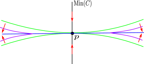
Figure 8. The level sets of the systole function passing through the critical point are shown in green. A level set at higher value of $f_{\mathrm{sys}}$ is shown in violet. The red arrows show the direction in which $f_{\mathrm{sys}}$ is increasing. The simplices $\sigma_{1}$ and $\sigma_{2}$ are shown in blue.

For $p$ in $\overline{\mathrm{Sys}(C)}$, the tangent cone to $\mathrm{Sys}(C)$ at $p$ will be denoted by $TC_{p}\mathrm{Sys}(C)$. If $p$ is a critical point of index $j$, and $C$ is the set of systoles at $p$, a descendent $C^{\prime}$ of $C$ is a subset of $C$ with the following properties

1. $C^{\prime}$ is eutactic at $p$

2. The span of $\{\nabla L(c)\ |\ c\in C^{\prime}\}$ is equal to the span of $\{\nabla L(c)\ |\ c\in C\}$

3. $C^{\prime}$ does not have a proper subset satisfying the first two conditions.

Note that the cardinality of a descendent $C^{\prime}$ is $j+1$. A subdescendent is the same as a descendent except it does not satisfy condition (2).

Theorem 22.

Fix a critical point $p\in\mathcal{P}_{g}$ of index $j$ with set of systoles $C$. (a) Then a neighbourhood of $p$ in $\mathcal{P}_{g}$ contains a piecewise smooth cell of codimension $j$ on which $f_{\mathrm{sys}}$ is increasing to second order away from the critical point. The tangent space of this cell at $p$ is in $\{\nabla L(c)(p)\ |\ c\in C\}^{\perp}$. (b) Moreover, the intersection of the cone of increase with the $\epsilon$-tangent cone to $\mathcal{P}_{g}$ at $p$ is stably connected.

In addition to proving the theorem, the following argument gives a model for $\mathcal{P}_{g}$ around a critical point, relating the geometry and the combinatorics. If the reader is not interested in the latter, the theorem also follows from the arguments in the previous section, with only minor adjustments.

Proof.

By local finiteness, convexity of length functions and the definition of $\mathrm{Min}(C)$, all the directions in which $f_{\mathrm{sys}}$ is increasing at $p$ to second order are contained in $\{\nabla L(c)(p)\ |\ c\in C\}^{\perp}$. At $p$, these directions are tangent to the level set of $f_{\mathrm{sys}}$ containing $p$. Recall that there exists a triangulation of $\mathcal{P}_{g}$ compatible with the stratification. Denote by $\sigma=\cup_{i=1}^{n}\sigma_{i}$ the union of simplices for which $TC_{p}\sigma=\{\nabla L(c)(p)\ |\ c\in C\}^{\perp}$. Note that existence of $\sigma$ is guaranteed by two observations: firstly, every vector in the cone of increase at $p$ is in $\{\nabla L(c)\ |\ c\in C\}^{\perp}$ and hence tangent to the level sets passing through $p$. Secondly, the restriction of $f_{\mathrm{sys}}$ to the interior of a stratum or a simplex is smooth, so the restriction of the level sets to the interiors of the simplices can only contain the smooth pieces of the piecewise smooth level sets. This is illustrated schematically in Figure 8.

For the purposes of constructing a combinatorial model of $\mathcal{P}_{g}$ around $p$, it is helpful to separately consider two cases. To begin with, it will be assumed that $\sigma$ has codimension $j$. Figure 8 shows an example satisfying this assumption, and Figure 9 shows one that does not.

It will now be shown that, on a neighbourhood of $p$, $\sigma$ is contained in $\mathcal{P}_{g}$. Note that each of $\sigma_{1},\ldots,\sigma_{n}$ is necessarily contained in a balanced locus as will now be explained. Let $x$ be a point in the interior of a simplex $\sigma_{i}$ in $\sigma$ where the systoles on $\sigma_{i}$ are given by $C_{i}\subset C$, and let $V$ be the subspace of $T_{x}\mathcal{T}_{g}$ given by the orthogonal complement of $v_{C_{i}}(x)$. Any vector in $V$ is either tangent to a level set of $\sigma_{i}$ or to a geodesic $\gamma$ with $\gamma(0)=x$ passing through level sets below $x$ for $t\in(-\epsilon,\epsilon)$. It follows from local finiteness that $\sigma_{i}$ is $V$-eutactic, and hence balanced.

Let $C_{i}=\{c_{1},\ldots,c_{k}\}$ be the systoles on $\sigma_{i}$ and consider a sequence of points in $\sigma_{i}$ approaching $p$. The stratum $\sigma_{i}$ is traced out by a 1-parameter family of faces of level sets above $p$ only, so in the limit as $p$ is approached, $f_{\mathrm{sys}}|_{\sigma_{i}}$ is increasing only to second order. At points in the sequence, the balanced sets of gradients $\{\nabla L(c)\ |\ c\in C_{i}\}$ become arbitrarily close to being eutactic. This implies that $C_{i}$ is a filling set, since otherwise a contradiction is obtained by invoking Proposition 3 and observing that in the limit as $p$ is approached, the open cone of directions in which the lengths of curves in $C_{i}$ are increasing is empty. This concludes the proof that $\sigma\subset\mathcal{P}_{g}$.

Let $C^{\prime}$ be a descendent of $C$. On a neighbourhood of $p$, $E(C^{\prime})$ is an embedded submanifold of codimension $j$, intersecting $\mathrm{Min}(C)$ in the unique point $p$. This follows from the fact that $\left\{\left(\nabla L(c_{2})-\nabla L(c_{1})\right),\ldots,\left(\nabla L(c_{k})-\nabla L(c_{1})\right)\right\}$ are linearly independent on a neighbourhood of $p$. The point $p$ is a minimum of the restriction to $E(C^{\prime})$ of the lengths of curves in $C^{\prime}$, and $T_{p}E(C^{\prime})$ is given by $\{\nabla L(c)(p)\ |\ c\in C^{\prime}\}^{\perp}=\{\nabla L(c)(p)\ |\ c\in C\}^{\perp}$.

Claim: Recalling the assumption that $\sigma$ has codimension $j$, on a neighbourhood of $p$, the codimension $j$ simplices $\sigma_{1},\ldots,\sigma_{n}$ are contained in loci labelled by descendents and unions of descendents.

To prove the claim, first note that balanced strata above $p$ can only be labelled by subsets of $C$ that are eutactic at $p$. This is because if $C_{i}\subset C$ is not eutactic, the balanced assumption implies that $v_{C_{i}}(p)\in TC_{p}\mathrm{Sys}(C_{i})$ is a direction in which the lengths of curves in $C^{\prime}$ are increasing to first order. For a point $x$ in $\sigma_{i}$ above $p$, local finiteness implies that $-v_{C_{i}}(x)\in TC_{x}\mathrm{Sys}(C_{i})$. As $x$ can be made arbitrarily close to $p$, this contradicts the assumption that $\sigma$ has codimension $j$.

Since $\mathrm{Sys}(C_{1}),\ldots,\mathrm{Sys}(C_{n})$ were shown to be balanced, condition 2 of the definition of descendents then implies that the only subsets of $C$ that could be systoles on codimension $j$ strata $\sigma_{i}$, $i=1,\ldots,n$ are descendents and unions of descendents. This concludes the proof of the claim.

When $C$ has more than one descendent, as in the example in the next subsection, exactly which descendents are realised as systoles depends on second order behaviour.

The assumption that $\sigma$ has codimension $j$ will now be dropped. Let $\sigma_{i}$ be a simplex in $\sigma$ of codimension less than $j$ that is not a face of a larger dimensional simplex of $\sigma$. Then at a point $x$ in the interior of $\sigma_{i}$ in a sufficiently small neighbourhood of $p$, $\mathrm{Sys}(C_{i})$ is balanced. This follows from the same argument as in the case when the codimension of $\sigma$ was assumed equal to $j$, the only difference is that the vector space $V\in T_{x}\mathcal{T}_{g}$ contains vectors tangent to level sets of $f_{sys}$ that are close to being parallel to vectors in the tangent space to $\mathrm{Min}(C)$ at $p$. More precisely, the span of $\{\nabla L(c)(x)\ |\ c\in C_{i}\}$ has codimension less than $j$. Since $\mathrm{Sys}(C_{i})$ is balanced in the intersection with a neighbourhood of $p$, it follows from the same argument as above that $\mathrm{Sys}(C_{i})\subset\mathcal{P}_{g}$. Since $\mathcal{P}_{g}$ is closed, $\sigma\subset\mathcal{P}_{g}$.

Mostly $C$ does not have subdescendents. In the abscence of subdescendents, $\sigma$ cannot contain any strata of codimension less than $j$. Any top dimensional strata in $\sigma$ were shown to be balanced, and hence labelled by subsets of $C$ that are eutactic at $p$. Without subdescendents, any subset of $C$ that is eutactic at $p$ can determine a stratum of codimension no less than $j$ at $p$.

When there exists a subdescendent $C^{\prime\prime}\subsetneq C$, there can also be a stratum $\mathrm{Sys}(C^{\prime\prime})$ in $\sigma$ with $p\in\overline{\mathrm{Sys}(C^{\prime\prime})}$ or a stratum with systoles given by a union of subdescendents. Although $\mathrm{Sys}(C^{\prime\prime})$ can have larger dimension than a stratum of descendents, as shown in Figure 9, it is “pinched” near $p$ (in the language of the previous section, it is traced out by a 1-parameter family of collapsing faces), so $TC_{p}\mathrm{Sys}(C^{\prime\prime})$ is also contained in $\{\nabla L(c)(p)\ |\ c\in C\}^{\perp}$. In this case, the simplices $\sigma_{1},\ldots,\sigma_{n}$ strictly contain a piecewise smooth cell of codimension $j$, with tangent space at $p$ given by $\{\nabla L(c)(p)\ |\ c\in C\}^{\perp}$. This concludes the proof of part (a).

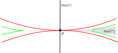
Figure 9. An example with a subdescendent $C^{\prime\prime}\subset C$. The level set of $f_{\mathrm{sys}}$ passing through $p$ is shown in red, and a level set above this in green.

Part (b) of the theorem follows from the wedge argument. Note that in this case, the cone of increase at $p$ is $S^{6g-6-j}\times\mathbb{R}$, so one only has stable connectivity and not stable contractibility of the intersection ($S^{6g-6-j}$) of the cone of increase with the $\epsilon$-tangent cone to $\mathcal{P}_{g}$ at $p$. ∎

Remark 23.

Theorem 22 implies that

$$\text{ codimension of }\mathcal{P}_{g}\leq|C|-1\text{ \ \ \ or \ \ \ dimension of }\mathcal{P}_{g}\geq 6g-|C|-5$$

This does not require Theorem 1 or Thurston’s construction from [16]. As explained in the proof of Theorem 22, it is a corollary of Proposition 3 and the characterisation of critical points given in [1] that the union of strata with tangent cone at $p$ given by $\{\nabla L(c)\ |\ c\in C\}^{\perp}$ is in $\mathcal{P}_{g}$. It then follows immediately from the sequence of critical points constructed in [6] that

$$\liminf_{g\rightarrow\infty}\frac{\text{dimension of }\mathcal{P}_{g}}{g}=0$$

This was proven in [12] by generalising an argument from [6].

Boundary points of the systole function and their structure. Recall that a boundary point of $f_{\mathrm{sys}}$ is a point at which $\mathrm{Sys}(C)$ intersects $\mathrm{Min}(C^{\prime})$, for $C^{\prime}\subsetneq C$. Since $\mathrm{Min}(C^{\prime})$ is empty unless $C^{\prime}$ fills, boundary points of $f_{\mathrm{sys}}$ are all necessarily contained in $\mathcal{P}_{g}$. Boundary points of $f_{\mathrm{sys}}$ were also shown in [14] to be isolated and hence there are at most finitely many modulo the action of $\Gamma_{g}$.

A boundary point of $f_{\mathrm{sys}}$ is not a critical point, but it also has no open cone in which $f_{\mathrm{sys}}$ is increasing. The level sets intersect as illustrated in Figure 10. The function $f_{\mathrm{sys}}$ increases away from a boundary point of $f_{\mathrm{sys}}$ only to second order.

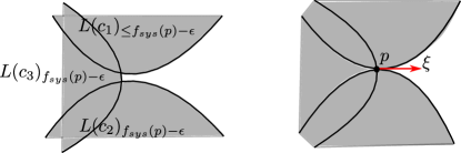
Figure 10. The intersection of level sets near a boundary point $p$ of $f_{\mathrm{sys}}$. The vector $\xi$ shows a direction in which $f_{\mathrm{sys}}$ is increasing away from $p$ to second order.

Ignoring the curves in $C{\smallsetminus}C^{\prime}$, around $p$, it is possible to construct the same simplices $\sigma_{1},\ldots,\sigma_{n}$ as in Theorem 22. For any vector in the tangent cone to $\sigma$ at $p$ giving a direction in which the length of a curve in $C{\smallsetminus}C^{\prime}$ is decreasing away from $p$, the set of systoles is in $C{\smallsetminus}C^{\prime}$. In all other directions near $p$, the behaviour of $f_{\mathrm{sys}}$ is identical to that near a critical point. Note that all directions in which $f_{\mathrm{sys}}$ is increasing away from $p$ are in the tangent cone to $\mathcal{P}_{g}$ at $p$.

6. Example: Schmutz’s critical point

The purpose of this subsection is to discuss an application of Theorem 22 in understanding the geometry of $\mathcal{P}_{2}$. This critical point is due to Schmutz [14] and is the first of a family of examples, one in each genus, of critical points of coindex equal to the virtual cohomological dimension of the mapping class group. This family of examples plays a key role in the study of the Steinberg module, [8].

Figure 11. The set of systoles at the critical point in the example are shown on the right. The left side of the figure shows a fundamental domain with edges lying along the systoles, and with numbers indicating the glung maps (not the labels of the curves). This figure is taken from [8].

Let $C$ be the set of curves on the right hand side of Figure 11. It was shown in Theorem 36 of [14] that there is a critical point $p$ of index 3 at which this set of curves is realised as the set of systoles. At $p$, the systoles intersect at right angles, cutting the surface into four regular hexagons. In [14], it was shown that $\mathrm{Min}(C)$ is a cell of dimension 3 with empty boundary.

Deleting any pair of intersecting curves in $C$ gives a minimal set of filling curves, all of which are descendents of $C$. The descendents are therefore

$$C_{1}=\{c_{1},c_{2},c_{3},c_{4}\}\ \ \ \ \ \ \ \ \ \ C_{2}=\{c_{2},c_{3},c_{4},c_{5}\} C_{3}=\{c_{3},c_{4},c_{5},c_{6}\}$$

$$C_{4}=\{c_{4},c_{5},c_{6},c_{1}\}\ \ \ \ \ \ \ \ \ \ C_{5}=\{c_{5},c_{6},c_{1},c_{2}\} C_{6}=\{c_{6},c_{1},c_{2},c_{3}\}$$

In this example there are no subdescendents.

For each descendent $C_{i},i=1,\ldots,6$ the locus $E(C_{i})$ is an embedded submanifold of dimension 3, intersecting $\mathrm{Min}(C)=\mathrm{Min}(C_{i})$ in the single point $p$, with $T_{p}E(C_{i})$ given by $\{\nabla L(c)\ |\ c\in C_{i}\}^{perp}=\{\nabla L(c)\ |\ c\in C\}^{\perp}$. This follows from the results in Section 3, or on a neighbourhood of $p$ by the rank calculations in [14].

Near $p$, $\mathcal{P}_{g}$ could potentially lie along any $E(C_{i})$; this is determined by second order behaviour. It is a consequence of the main construction in [12] that $E(C)=\cap_{i=1}^{i=6}E(C_{i})$ has a connected component consisting of a one dimensional embedded submanifold of $\mathcal{T}_{g}$ containing $p$. On a neighbourhood of $p$, by local finiteness, the points of $E(C)$ are in $\mathrm{Sys}(C)$. The same construction from [12] also implies that every proper filling subset of $C$ determines a stratum of $\mathcal{P}_{g}$ adjacent to $E(C)$; these are arranged as shown in Figure 12.

Figure 12. The arrangement of strata in $\mathcal{P}_{2}$ on a neighbourhood of the critical point $p$ in the example. The 3-sphere is piecewise smooth, and has a symmetry group given by the dihedral group $D_{6}$ that acts transitively on the top dimensional strata of $\mathcal{P}_{2}$ adjacent to $p$.

The automorphism group of the hyperbolic surface corresponding to $p$ contains a subgroup of the mapping class group isomorphic to the dihedral group $D_{6}$, and the connected component of the locus $E(C)$ passing through $p$ is the fixed point set of this subgroup. It follows that this connected component of $E(C)$ is a geodesic with respect to any mapping class group-equivariant metric on $\mathcal{T}_{g}$, such as the Teichmüller metric or the Weil-Petersson metric.

The set of minima $\mathrm{Min}(C)$ also has a simple parameterisation. In genus 2, $\mathrm{Min}(C)$ is the set of points at which the curves in $C$ intersect at right angles.

Theorem 24 (Ratcliffe, Theorem 3.5.14).

For any $a,b,c\in\mathbb{R}^{+}$ there is a right-angled hyperbolic convex hexagon, unique up to congruence, with alternate sides of length $a,b$ and $c$.

Using Theorem 24, from the left side of Figure 11, it is not difficult to verify that by Theorem 24 the lengths of 3 alternate edges of any one of the hexagons of $S_{g}{\smallsetminus}C$ completely parameterise $\mathrm{Min}(C)$.

References

- [1] H. Akrout. Singularités topologiques des systoles généralisées. Topology, 42(2):291–308, 2003.
- [2] A. Barvinok. Lattice points, polyhedra, and complexity. In Geometric combinatorics, volume 13 of IAS/Park City Math. Ser., pages 19–62. American Mathematical Society, Providence, RI, 2007.
- [3] L. Bers. Nielsen extensions of Riemann surfaces. Annales Academiæ Scientiarum Fennicæ, Series A. I. Mathematica, 2:29–34, 1976.
- [4] L. Bers. An Inequality for Riemann Surfaces, pages 87–93. Springer Berlin Heidelberg, Berlin, Heidelberg, 1985.
- [5] M. Bestvina, K. Bromberg, K. Fujiwara, and J. Souto. Shearing coordinates and convexity of length functions on Teichmüller space. American Journal of Mathematics, 135(6):1449–1476, 2013.
- [6] M. Fortier Bourque. The dimension of Thurston’s spine. arXiv:2211.08923, 2022.
- [7] M. Brion and M. Vergne. Lattice points in simple polytopes. Journal of the American Mathematical Society, 10(2):371–392, 1997.
- [8] I. Irmer. An explicit generating set for the Steinberg module of the mapping class group. arXiv:2312.08721, 2023.
- [9] S. Kerckhoff. The Nielsen realization problem. Annals of Mathematics, 117(2):235–265, 1983.
- [10] J. Lee. Introduction to smooth manifolds, 2nd Edition, volume 218 of Graduate Texts in Mathematics. Springer, New York, 2013.
- [11] S. Lojasiewicz. Triangulation of semi-analytic sets. Annali della Scuola Normale Superiore di Pisa - Classe di Scienze, 18(4):449–474, 1964.
- [12] O. Mathieu. Estimating the dimension of the Thurston spine. arXiv:2310.15618, 2023.
- [13] M. Morse. Topologically non-degenerate functions on a compact -manifold . Journal d’Analyse Mathématique, 7:189–208, 1959.
- [14] P. Schmutz Schaller. Systoles and topological Morse functions for Riemann surfaces. Journal of Differential Geometry, 52(3):407–452, 1999.
- [15] P. Schmutz Schaller. Riemann surfaces with longest systole and an improved Voronoĭ algorithm. Archiv der Mathematik, 76(3):231–240, 2001.
- [16] W. Thurston. A spine for Teichmüller space. Preprint, 1985.
- [17] S. Wolpert. An elementary formula for the Fenchel-Nielsen twist. Commentarii Mathematici Helvetici, 56(1):132–135, 1981.
- [18] S. Wolpert. Geodesic length functions and the Nielsen problem. Journal of Differential Geometry, 25(2):275–296, 1987.