Field theory expansions of string theory amplitudes

Abstract

It is commonly believed that string theory amplitudes cannot be expanded in terms of poles of all channels, thereby distinguishing them from the usual Feynman diagram expansion in quantum field theory. We present here new representations of the Euler-Beta function and tree-level string theory amplitudes which are analytic everywhere except at the poles but sum over poles in all channels, and, crucially, include contact diagrams, very much in the spirit of quantum field theory. This enables us to consider mass-level truncation, which preserves all the features of the original amplitude. By starting with such expansions for generalized Euler-Beta functions and demanding QFT like features, we single out the open string amplitude. Our considerations also lead to new field theory inspired representations of the Zeta function, which have very fast convergence. We demonstrate the difficulty in deforming away from the string amplitude and show that a class of such deformations can be potentially interesting when there is level truncation.

I Introduction

It is often said that string theory amplitudes are very different from quantum field theory (QFT) amplitudes [1, 2]. For instance, they exhibit Regge behaviour and exponentially soft high energy behaviour at fixed angle scattering. Further, it is also commonly held that string theory amplitudes, for instance for 2-2 scattering with two channels, can only be expanded in the poles of one channel but not all, as the sum over poles in one channel would automatically produce the poles in the other channel. This would give the impression, that we cannot write down a field theory representation of such amplitudes, where we have cubic vertices for the higher spin massive exchanged particles and (potential) contact diagrams. To be precise, we would like to truncate such an expansion up to some mass level. To capture the essential features of the string amplitude, like the exponentially soft high energy behaviour or the Regge behaviour up to some energy scale, if we had to retain a very large number of mass levels, much bigger than this energy scale, we would not call this field theory. We already know that there exists a perfectly valid and well understood low energy limit, where the energy scale is much smaller than the inverse string length, and where the description is via a low energy effective action in QFT. Further, string field theory hints at the existence of a field theory like representation of string amplitudes, not just at low energies but including the higher mass poles–we will review this below. In this letter, we demonstrate that there indeed exists such a field theory representation of 2-2 string amplitudes, which enables us to truncate in mass-levels, while retaining all the properties of the string amplitudes.

We begin by reviewing some well-known and some not-so-well-known facts. The Euler Beta function, introduced by Euler in the 18th century, has the integral representation:

$$B(-s_{1},-s_{2})=\frac{\Gamma(-s_{1})\Gamma(-s_{2})}{\Gamma(-s_{1}-s_{2})}=\int_{0}^{1}dz\,z^{-s_{1}-1}(1-z)^{-s_{2}-1}\,.$$ (1)

This integral form connects up with a world-sheet description. The convergence of the integral requires ${\rm Re}(s_{1})<0$ and ${\rm Re}(s_{2})<0$. For other $s_{1},s_{2}$ it is defined via analytic continuation and is given by the Gamma function form. It is also well-known that the Beta function can be expanded in terms of the $s_{1}$ or $s_{2}$ poles:

$$B(-s_{1},-s_{2})=-\frac{1}{s_{1}}-\sum_{n=1}^{\infty}\frac{1}{n!}\frac{(s_{2}+1)_{n}}{s_{1}-n}\,,$$ (2)

which converges for ${\rm Re}(s_{2})<0$. Here $(a)_{b}=\Gamma(a+b)/\Gamma(a)$ is the Pochhammer symbol. For $b=n\geq 0$ and integer, a degree $n$ polynomial in $(a+b)$ is obtained. A similar expression exists with $s_{1},s_{2}$ interchanged. This very property was responsible for the birth of string theory via the Veneziano amplitude [1, 2]. Dual resonance models posit that the amplitude can be expanded in terms of the poles of either channels but not both—purportedly distinguishing themselves from quantum field theories where we expand in terms of the poles in all channels.

It is less well-known that the Euler Beta function also has the integral representation [3]:

$$B(-s_{1},-s_{2})=\int_{0}^{1}dz\,\frac{z^{-s_{1}-1}+z^{-s_{2}-1}}{(1+z)^{-s_{1}-s_{2}}}\,,$$ (3)

which converges when ${\rm Re}(s_{1}),{\rm Re}(s_{2})<0$. If we expand the denominator around $z=0$ and integrate term by term, we will get an analytically continued representation in terms of the sum over poles in both $s_{1},s_{2}$, albeit one which only works in a limited regime:

$$\sum_{n=0}^{\infty}\left(\frac{1}{n-s_{1}}+\frac{1}{n-s_{2}}\right)\frac{(s_{1}+s_{2}-n+1)_{n}}{n!}\,,$$ (4)

where the summand for large $n$ goes like $n^{-2-s_{1}-s_{2}}$ needing ${\rm Re}(s_{1}+s_{2})>-1$ for convergence. Contrary to what is frequently mentioned in the older literature, this form, which sums over poles in both channels does not have any “double-counting”—the crucial, implicit contact terms in this representation avoid this. However, the restriction ${\rm Re}(s_{1}+s_{2})>-1$ is undesirable since in tree-level QFT, we do not expect any further singularities in the complex $s_{1},s_{2}$-plane except at the poles in all channels. Thus, while promising, this representation is still not what we would identify with QFT.

Now, string field theory numerical calculations in [4, 5] suggest that a mass-level expansion with the following properties should exist: (i) We sum over poles in all channels, introducing no new singularities except at these poles. (ii) Contact terms are crucial and finite; their precise form is subject to field redefinition ambiguity. (iii) The field redefinition ambiguity shows up in the truncated expansion. This last point will play a very important role in what follows. Unfortunately, such an analytic representation has never been worked out in the literature . Using the recently revived interest in crossing symmetric dispersion relations, attempts have been made to write string amplitudes as poles over all channels [7, 8, 9]. However, none of these satisfy all the criteria mentioned above (eg. (iii)) and do not allow for a convenient truncation, which would retain all the features of the string amplitude. Would such a representation look like QFT involving higher-spin massive particles? In particular, suppose we were interested in the physics inside $|s_{1,2}|<R$, then would we be able to capture all the important features of the string amplitude by retaining $N\sim R$ modes and including contact terms that exhibit finiteness? What we mean by the finiteness of the contact terms is that as we add more modes into the description, the coefficients in front of the contact term polynomials exhibit signs of convergence. We will show that there indeed exist new representations of string amplitudes with these QFT inspired properties. Rather fascinatingly, we will also demonstrate that for massless 2-2 scattering, we are naturally led to the open superstring amplitude using these considerations.

II Generalized Euler-Beta function

We start with a generalised version of the Veneziano amplitude/Euler-Beta function given by $\frac{\Gamma\left(\alpha-s_{1}\right)\Gamma\left(\alpha-s_{2}\right)}{\Gamma\left(\beta-s_{1}-s_{2}\right)}$. Using a local two-channel crossing symmetric dispersion relation, which can be worked out by using [11] and extending [12], this amplitude can be recast as a summation over the $s_{1},s_{2}$ poles in the following way,

$$\frac{\Gamma\left(\alpha-s_{1}\right)\Gamma\left(\alpha-s_{2}\right)}{\Gamma\left(\beta-s_{1}-s_{2}\right)} = \sum_{n=0}^{\infty}\frac{1}{n!}\left(\frac{1}{s_{1}-\alpha-n}+\frac{1}{s_{2}-\alpha-n}+\frac{1}{\alpha+\lambda+n}\right)\frac{\sin\left[\pi\left(\alpha-\beta-\lambda+\frac{\left(s_{1}+\lambda\right)\left(s_{2}+\lambda\right)}{\alpha+\lambda+n}\right)\right]}{\sin\left[\pi\left(\alpha+\lambda-\frac{\left(s_{1}+\lambda\right)\left(s_{2}+\lambda\right)}{\alpha+\lambda+n}\right)\right]}$$ (5)

$$\times\left(1-\alpha-\lambda+\frac{\left(s_{1}+\lambda\right)\left(s_{2}+\lambda\right)}{\alpha+\lambda+n}\right)_{n+2\alpha-\beta}$$

We derive this in the appendix. The extra parameter $\lambda$, which does not appear on the lhs and which mimics the expected field redefinition ambiguity, can be incorporated seamlessly. Without $\lambda$, we would not have a QFT like representation of the amplitudes, since as one can verify with (6), we would fail to capture the exponentially soft behaviour using a mass-level truncation. The familiar Euler-Beta function is obtained by choosing $\alpha=\beta=0$,

$$\frac{\Gamma\left(-s_{1}\right)\Gamma\left(-s_{2}\right)}{\Gamma\left(-s_{1}-s_{2}\right)} = -\sum_{n=0}^{\infty}\frac{1}{n!}\left(\frac{1}{s_{1}-n}+\frac{1}{s_{2}-n}+\frac{1}{\lambda+n}\right)$$ (6)

$$\left(1-\lambda+\frac{\left(s_{1}+\lambda\right)\left(s_{2}+\lambda\right)}{\lambda+n}\right)_{n}.$$

Each level can be expressed as terms containing poles at $s_{1}$ and $s_{2}$ channel and contact terms. For example, the first two levels are given by

$$n=0 : -\frac{1}{s_{1}}-\frac{1}{s_{2}}-\frac{1}{\lambda},$$ (7)

$$n=1 : -\frac{1+s_{2}}{s_{1}-1}-\frac{1+s_{1}}{s_{2}-1}-1-\frac{\lambda^{2}+\left(2\lambda+1\right)x+y}{(\lambda+1)^{2}},$$

where we define $s_{1}+s_{2}=x$ and $s_{1}s_{2}=y$. The polynomials in $x,y$ are the contact terms. This suggests that a potential Lagrangian description exists for 2-2 scattering of massless scalars, $\Phi$ with massive higher spin exchanges, $\mathbf{S_{\mu_{1}\cdots\mu_{\ell}}}$ at every level $n$,

$$\mathcal{L}_{n}\sim\sum_{\ell=0}^{n}\Phi\partial^{\mu_{1}\cdots\mu_{\ell}}\Phi\mathbf{S}_{\mu_{1}\cdots\mu_{\ell}}+\sum_{j=0}^{4n}\bigl{\{}\partial^{j}\bigr{\}}\Phi^{4}.$$ (8)

As will be elucidated in the rest of the paper, our objective is to obtain a QFT-like form by summing over $\mathcal{L}_{n}$, retaining only a finite number of terms in the series.

III Open string amplitude

We will now show that QFT considerations pick $\alpha,\beta$ for the open superstring amplitude. For the convergence of the $n$-sum in the above equation, we need $\alpha-\beta-\lambda<0$. Note that this condition is independent of $s_{1},s_{2}$, unlike the representations discussed in the Introduction. Further, notice that the trigonometric factor would imply an infinite number of contact terms at each mass level. To avoid this possiblity, we need $2\alpha-\beta=p$, where $p$ is any integer, whereby the trigonometric factor reduces to $(-1)^{p+1}$. This also leads to the Pochhammer term for $n+p\geq 0$ becoming a degree $n+p$ polynomial in $s_{1},s_{2}$; when $n+p<0$, we get poles from the Pochhammer. For instance, if $n=1,p<-1$, we would have higher order poles in the amplitude, which we will assume to be absent in a local theory. This leads to $p\geq-1$. Negative values of $\alpha$ correspond to tachyonic exchanges. We will focus on the situation where there are no tachyonic states. For the presence of a massless pole, $\alpha=0$. This, together with $2\alpha-\beta=p\geq-1$ leaves $\beta\leq 1$ and integer as the only possibility. Now, for a field theory representation we expect the contact terms to be finite. The $n$-dependence of the contact terms is $n^{-1+\alpha-\beta}$ so that for convergence we have $\beta>\alpha$. For $\alpha=0$, this uniquely picks out $\beta=1$. This is precisely the open superstring amplitude! For example, this amplitude describes the scattering of gluons after dressing with a kinematic factor $t_{8}{\rm Tr}F^{4}$, with the trace being over the gauge indices and the $t_{8}$ giving the contraction of the spatial indices [13]. We obtained this without appealing to unitarity or a world-sheet description. In recent literature, there have been attempts to zoom in to the open string amplitude using world-sheet monodromy constraints [14].

The convergence of the $n$-sum (for $\alpha=0,\beta=1$) in eq.(5) now tells us that $\lambda>-1$. Quite nicely, the $n=0$ term gives $1/(s_{1}s_{2})$, with no $\lambda$-dependence. The $\lambda$-dependence in the other levels cancels out when we sum over all poles. This is a non-trivial check of the correctness of the representation. Furthermore, as in field theory, in a truncated sum, the $\lambda$-dependence is simply reflective of the field redefinition ambiguity. Therefore, the four-point open string amplitude takes the form,

$$\frac{\Gamma\left(-s_{1}\right)\Gamma\left(-s_{2}\right)}{\Gamma\left(1-s_{1}-s_{2}\right)} = \sum_{n=0}^{\infty}\frac{1}{n!}\left(\frac{1}{s_{1}-n}+\frac{1}{s_{2}-n}+\frac{1}{\lambda+n}\right)\left(1-\lambda+\frac{\left(s_{1}+\lambda\right)\left(s_{2}+\lambda\right)}{\lambda+n}\right)_{n-1}.$$ (9)

Note here that if we fix the level number and take $\lambda\gg 1$, then the representation is similar to that in eq.(4). The salient features of the above representation of the four-point open string amplitude are the following: (i) It contains terms which are manifestly crossing symmetric at each mass level. Hence, exchange diagrams in both $s_{1}$ and $s_{2}$ channels along with the contact interactions can be discerned easily. (ii) For a range of the parameter $\lambda$ , if we truncate the series in the RHS of Eq.(9) to a finite mass level, then the truncated sum retains all the properties that the original amplitude has. We will now demonstrate this latter point. We will refer to the truncated sum as $M_{\text{T}}\left(s_{1},s_{2}\right)$ and number of terms in the sum by $N$.

III.1 Field theory analogue

Let us consider an energy scale $\Lambda$, such that $|s_{i}|<\Lambda^{2}$. Although the sum in Eq.(9) contains infinite number of terms, at the energy scale $\Lambda$ it suffices to truncate the sum to number of terms of $\mathcal{O}\left(\Lambda^{2}\right)$. In fig.(1), we exhibit evidence that the truncated expansion captures all the essential features of the actual amplitude, both in the physical region as well as in the unphysical region. The top panel is obtained using (9), truncated as indicated while the bottom is obtained using (4).

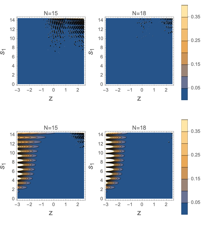
Figure 1: Plot showing fractional deviation of $M_{T}$ from the actual amplitude as function of $z=\cos\theta$ for the range of $s_{1}$. $N$ denotes the number of terms retained in the truncated sum. In the first row $\lambda=5.5$ and in the second row $\lambda\rightarrow\infty$.

III.1.1 Low energy expansion

The low energy expansion of the amplitude is given by

$$\mathcal{M}\left(s_{1},s_{2}\right) \approx \frac{1}{s_{1}s_{2}}-\zeta\left(2\right)-\zeta\left(3\right)\left(s_{1}+s_{2}\right)$$ (10)

$$-\zeta\left(4\right)\left(s_{1}^{2}+\frac{1}{4}s_{1}s_{2}+s_{2}^{2}\right)+\cdots$$

Working with $M_{\text{T}}\left(s_{1},s_{2}\right)$, the low energy behavior can be reproduced to an excellent accuracy. Numerical investigations suggest that for $\lambda\gtrsim 1$ with $N=20$ terms in the truncated sum, the agreement with the actual result is more than $99\%$. We demonstrate this in fig.(2). Here, we scaled $s_{1}$ and $s_{2}$ by $\epsilon$ and took the ratio $\left(r\right)$ of the low energy limit of $M_{\text{T}}$ to that of the actual amplitude at each order in $\epsilon$.

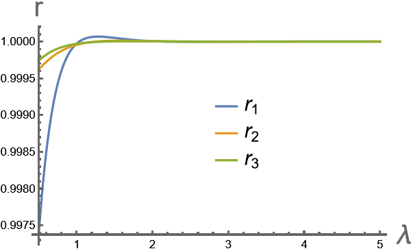
Figure 2: Ratio at each order in $\epsilon$ plotted as function of $\lambda$. $r_{1}$, $r_{2}$ and $r_{3}$ are the ratios at $\epsilon^{0}$, $\epsilon$ and $\epsilon^{2}$ respectively. Sum in $M_{\text{T}}$ is truncated at $N=20$.

In this way we can also deduce new identities for $\zeta$ functions. As an example, we present

$$-\sum_{n=1}^{\infty}\frac{(2\lambda+n)\Gamma\left(\frac{n^{2}}{n+\lambda}\right)}{\lambda n^{3}\Gamma(n)\Gamma\left(-\frac{n\lambda}{n+\lambda}\right)}=\zeta\left(2\right).$$ (11)

If we set $\lambda=0$, then the summand reduces to $\frac{1}{n^{2}}$. Convergence of the sum improves dramatically when $\lambda\neq 0$. Putting $\lambda=41.5$, we get convergence to 15 decimal places retaining only 40 terms, while $\sum 1/n^{2}$ would need 50 million terms! . To the best of our knowledge, such representations do not exist in the mathematics literature [17]. We give a similar representation for $\zeta(3)$ in the appendix.

III.1.2 Contact terms

Figure 3: Coefficients of contact terms appearing at $\mathcal{O}\left(s_{i}^{2}\right)$ plotted against $\lambda$. Sum is truncated at $N=20$

.

We denote the contact terms by $\left(-1\right)^{q}C_{pq}(s_{1}+s_{2})^{p}(s_{1}s_{2})^{q}$. We show in fig.(3) how the coefficients $C_{pq}$ change with $\lambda$. A distinct plateau appears with $\lambda$. These plateaus indicate that $\partial_{\lambda}M_{T}\approx 0$, which is exactly what we would want in the QFT representation.

III.1.3 Regge $\&$ Hard Scattering

Finally, we look at the high energy limits. In the Regge limit $s_{1}\rightarrow\infty$ keeping $s_{2}$ fixed, the amplitude is known to behave as $M\left(s_{1},s_{2}\right)\approx-s_{1}^{-1+s_{2}}\Gamma\left(-s_{2}\right)\frac{\sin\left(\pi\left(s_{1}+s_{2}\right)\right)}{\sin\left(\pi s_{1}\right)}.$ This is very accurately captured by the truncated representation as shown in fig.(4) upto (and a bit beyond) the truncation.

Figure 4: Absolute value of truncated amplitude with $s_{2}=-0.2$ for different values of $N$ plotted as function of $s_{1}+0.1i$. Here $\lambda=8.5$. The black curve represents the behavior of the actual amplitude.

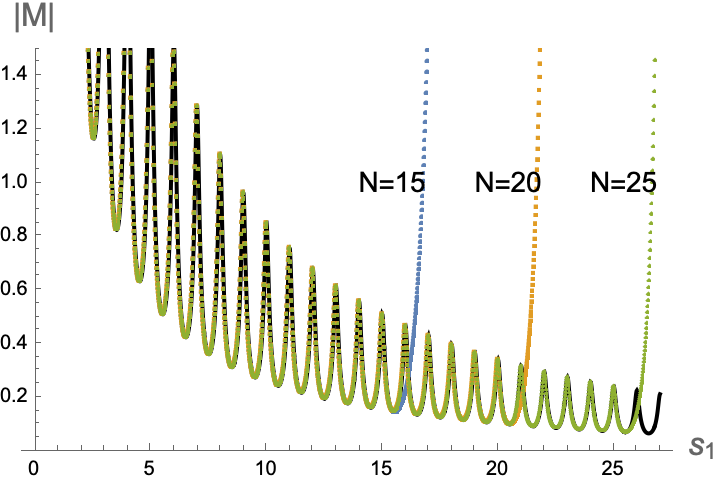
Figure 5: Absolute value of truncated amplitude with $z=-0.99$ for different values of $N$ plotted as function of $s_{1}+0.1i$. Here $\lambda=8.5$. The black curve represents the behavior of the actual amplitude.

The exponentially soft high energy, fixed angle ($z=1+2s_{2}/s_{1}$) scattering behaviour is a smoking gun for string theory. Remarkably, the truncated representation captures even this behaviour faithfully as shown in fig.(5).

IV Deformations

We now consider a certain deformation of the amplitude, retaining crossing symmetry and having the same spectrum. The simplest way to do this is to replace the $\frac{(s_{1}+\lambda)(s_{2}+\lambda)}{\lambda+n}$ in the Pochhammer by $\frac{(s_{1}+\lambda)(s_{2}+\lambda)}{c(\lambda+n)}$, with $c$ a deformation parameter. This changes the residues at the poles. When we examine the unitarity of the resulting partial waves, we find a restriction on $c$ and maximum $\lambda$ as depicted in the figure below. Unitarity restricts $c\geq 1$, while $\lambda$ is also restricted from above for $c>1$, unlike for $c=1$, where the residues are independent of $\lambda$. Curiously, $D=10$ exhibits a discontinuity in the plot as $\lambda_{max}$ changes from positive to negative near $c\sim 1$. Note that $D>10$ is now allowed by tree-level unitarity.

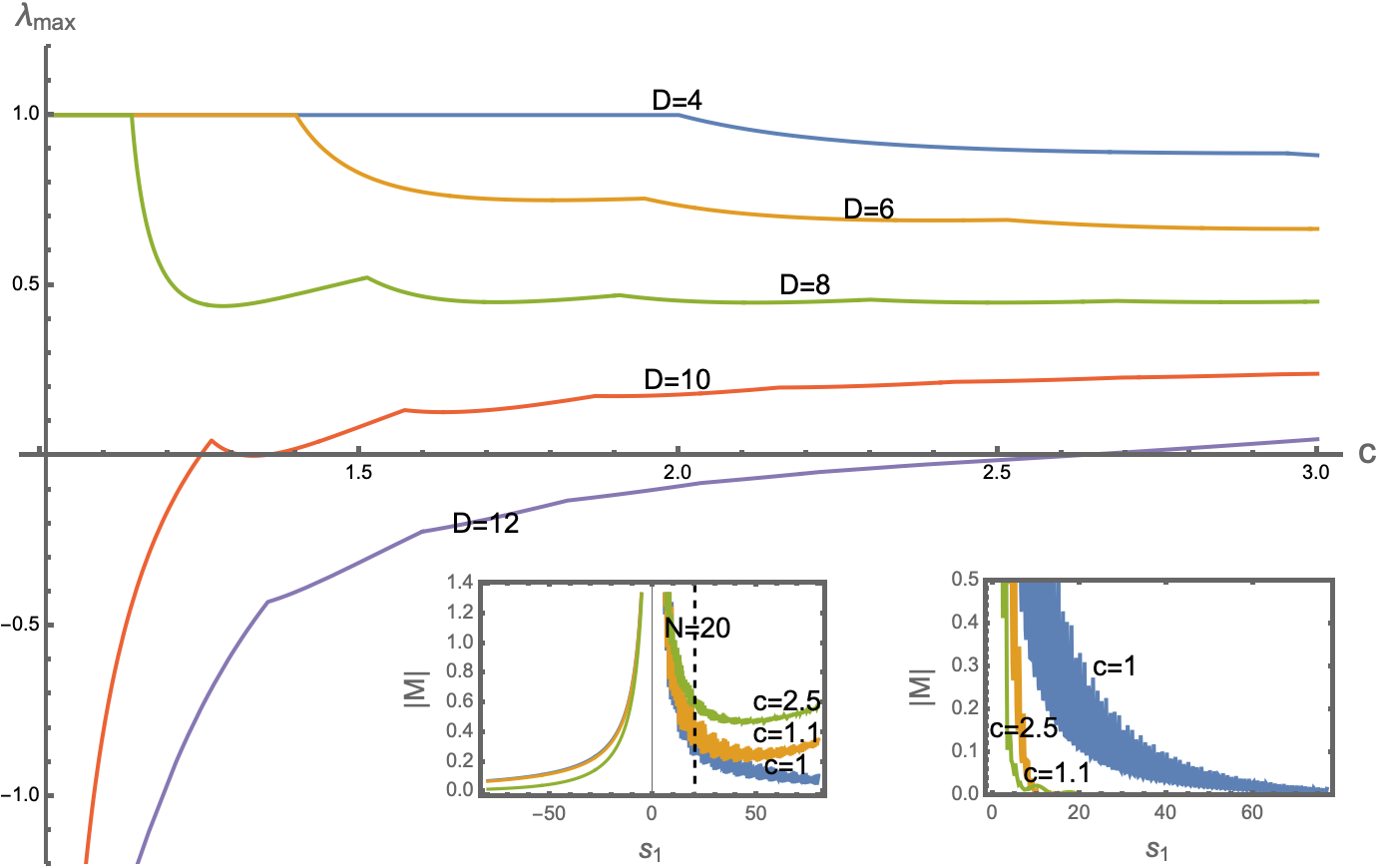
Figure 6: Tree level unitarity allows regions below the bounding lines for dimensions as indicated. Inset plots give Regge on the left and hard-scattering on the right. Here $\lambda=0.5,N=80$.

The most interesting question is if the level truncation is sensitive to the $c$-deformation or if there is some freedom which retains all the qualitative features at high energies for the amplitude. Our analysis of the high energy limits suggests that as soon as $c\neq 1$, the Regge behaviour is ruined beyond some energy scale. However, there appears to be some approximate sense in which both Regge and hard-scattering limits are similar to the stringy scenario up to some energy scale. We emphasise that the family of deformations we have considered does appear to single out the string theory answer, unless we restrict the energy scale. We will leave a more detailed study of deformations in the spirit of recent work [18, 19, 14] for the future.

V Discussion

There exist two well-studied limits of string theory where the string tension is either taken to infinity (eg.[1]) or zero (eg. [20]). The representations presented here can be used to study an intermediate limit, where the energy scale is such that only some of the higher spin massive modes are effectively massless. While the analysis above has focused on the open string, similar results hold also for the closed string. We briefly discuss this in the appendix. Does the truncated amplitude know about the underlying worldsheet? Note here that $\lambda$ in (9) is dimensionless. In string field theory a similar dimensionless parameter enters [5] in the plumbing fixture method, via a choice of local coordinates for fixed vertex operators on two glued discs/spheres. After a Mobius transformation, a one parameter ambiguity is left. The value of this parameter controls the rate of convergence of the level sum, very similar to what we have found here. Our explicit representation gives an analytic realization of the expectations from string field theory, and resolves certain confusing claims in the literature. One of the most exciting prospects of the new representations in this paper is to use suitable modifications of them to re-examine experimental data for hadron scattering.

In light of our findings, it will be interesting to re-examine [21], which discusses a no-go theorem for quantum field theories with massless higher spin exchanges. Another interesting direction to pursue is to extend existing on-shell techniques [22] to incorporate contact diagrams as suggested by the analysis in this paper. In particular, when we consider higher point functions, the contact diagrams would play an important role. In principle, one could start with the absorptive part of a four-point function and obtain the contact terms using the local crossing-symmetric dispersion relation. However, in practice, this is still a difficult program to implement, since this needs to be done for amplitudes more general than just identical particles.

Our new representation will also be useful in connecting with celestial holography [23]. In particular, it will be interesting to examine how the mass-level truncation and the exponential softness of the full amplitude manifest in the Celestial or Carollian CFTs.

Appendix A Crossing Symmetric Dispersion Relation

We briefly review the two-channel crossing symmetric dispersion relation for $2-2$ scattering obtained in [11]. The Mandelstam variables satisfy $s+t+u=\mu^{2}$. We define new variables: $s_{1}=s-\frac{\mu}{3}$, $s_{2}=t-\frac{\mu}{3}$ and $s_{3}=u-\frac{\mu}{3}$. $s_{1}$ and $s_{2}$ are mapped to complex $z$-plane using the following parameterization,

$$s_{k}=\frac{4aze^{i\pi k}}{\left(z+e^{i\pi k}\right)^{2}},\qquad k=1,2,$$ (12)

where $a=\frac{s_{1}s_{2}}{s_{1}+s_{2}}$ is held fixed. We assume that the amplitude in the Regge limit falls off as $|\mathcal{M}|\sim o(s_{1})$. Note that unlike the 3-channel case, where $s_{1}+s_{2}+s_{3}=0$, there is no restriction on $s_{1}+s_{2}$.

Discontinuities of the amplitude in the $s_{1}$-channel, for $s_{1}>a$, are located on the unit circle $|z|=1$ in the complex plane. Demanding that near $z=0$ the amplitude can be expanded in powers of only $z^{2}$, we obtain a dispersion relation,

$$\widetilde{\mathcal{M}}\left(z,a\right)=\widetilde{\mathcal{M}}\left(0,a\right)+\frac{1}{\pi}\frac{z^{2}}{1-z^{2}}\int_{|z^{\prime}|=1}\frac{\mathrm{d}z^{\prime}}{z^{\prime}}\frac{z^{{}^{\prime}2}-1}{z^{{}^{\prime}2}-z^{2}}\widetilde{\mathcal{A}}\left(z^{\prime},a\right).$$ (13)

Discontinuity of the amplitude at $z=1$ is defined as $\widetilde{\mathcal{A}}\left(z,a\right)=\lim_{\epsilon\rightarrow 0}\frac{1}{2i}\left[\widetilde{\mathcal{M}}\left(\left(1+\epsilon\right)e^{i\phi},a\right)-\widetilde{\mathcal{M}}\left(\left(1-\epsilon\right)e^{i\phi},a\right)\right]$, with $0\leq\phi\leq 2\pi$. Written in terms of the kinematic variables, Eq.(13) lead to the following two-channel crossing symmetric dispersion relation

$$\mathcal{M}\left(s_{1},s_{2}\right)=\mathcal{M}\left(0,0\right)+\frac{1}{\pi}\int_{a}^{\infty}\frac{\mathrm{d}\sigma}{\sigma}\mathcal{A}(\sigma,\frac{a\sigma}{\sigma-a})\left[\frac{s_{1}}{\sigma-s_{1}}+\frac{s_{2}}{\sigma-s_{2}}\right],$$ (14)

where the $\mathcal{A}(s_{1},s_{2})$ is the $s_{1}$-discontinuity of the amplitude. As it stands, this representation has non-local terms since Taylor expanding around $a=0$ leads to negative powers of $(s_{1}+s_{2})$. One can either remove these singularities imposing the so-called locality constraints, leading to what was dubbed as the Feynman block expansion in [7] or work out a more convenient local dispersion relation.

A.1 Local crossing symmetric dispersion relation

The kernel in Eq.(14) can be expressed as

$$H\left(\sigma;x,y\right)=\frac{\sigma^{2}-y}{\sigma^{2}-x\sigma+y}-1.$$ (15)

We follow a similar analysis done in [12] to eliminate negative exponents in $x$ from the dispersion relation. We perform a Taylor series expansion of $\mathcal{A}$ around $a=0$. Note that $ax=y$. Corresponding to $x^{n}$ we define a state $|n\rangle$ and $a$ is promoted to operator $\hat{a}$, such that $\hat{a}|n\rangle=|n-1\rangle$ and $\hat{a}|0\rangle=0$. Then it follows that $\hat{a}^{n}\frac{1}{\sigma^{2}-x\sigma+y}=\left(\frac{\sigma y}{\sigma^{2}+y}\right)^{n}\frac{1}{\sigma^{2}-x\sigma+y}$. This leads us to the following local dispersion relation,

$$\mathcal{M}^{(\text{local})}\left(s_{1},s_{2}\right)=\mathcal{M}\left(0,0\right)+\frac{1}{\pi}\int_{a}^{\infty}\frac{\mathrm{d}\sigma}{\sigma}\left[\frac{\sigma^{2}-y}{\sigma^{2}-x\sigma+y}\mathcal{A}\left(\sigma,\frac{y}{\sigma}\right)-\mathcal{A}\left(\sigma,0\right)\right].$$ (16)

Appendix B Generalised Euler-Beta function

We consider a generalisation of Veneziano amplitude of the form $\mathcal{M}\left(s_{1},s_{2}\right)=\frac{\Gamma\left(\alpha-s_{1}\right)\Gamma\left(\alpha-s_{2}\right)}{\Gamma\left(\beta-s_{1}-s_{2}\right)}$. For non-zero $\alpha$ and $\beta$, $\mathcal{M}\left(0,0\right)=\frac{\Gamma^{2}\left(\alpha\right)}{\Gamma\left(\beta\right)}$. Using Eq.(16) and $\sum_{n=0}^{\infty}\frac{\left(-1\right)^{n}}{n!\left(\alpha+n\right)}\frac{\Gamma(\alpha)}{\Gamma(-n-\alpha+\beta)}=\frac{\Gamma^{2}\left(\alpha\right)}{\Gamma\left(\beta\right)}$, we obtain the following series representation,

$$\frac{\Gamma\left(\alpha-s_{1}\right)\Gamma\left(\alpha-s_{2}\right)}{\Gamma\left(\beta-s_{1}-s_{2}\right)}=\sum_{n=0}^{\infty}\frac{(-1)^{n}}{n!}\left(\frac{1}{\alpha+n-s_{1}}+\frac{1}{\alpha+n-s_{2}}-\frac{1}{\alpha+n}\right)\frac{\Gamma\left(\alpha-\frac{s_{1}s_{2}}{n+\alpha}\right)}{\Gamma\left(-n-\alpha+\beta-\frac{s_{1}s_{2}}{n+\alpha}\right)}.$$ (17)

After using the identity, $\Gamma\left(x\right)\Gamma\left(1-x\right)=\frac{\pi}{\sin\left(\pi x\right)}$, the above equation can be expressed as

$$\frac{\Gamma\left(\alpha-s_{1}\right)\Gamma\left(\alpha-s_{2}\right)}{\Gamma\left(\beta-s_{1}-s_{2}\right)} = \sum_{n=0}^{\infty}\frac{1}{n!}\left(\frac{1}{s_{1}-\alpha-n}+\frac{1}{s_{2}-\alpha-n}+\frac{1}{\alpha+n}\right)$$ (18)

$$\hskip 85.35826pt\frac{\sin\left[\pi\left(\alpha-\beta+\frac{s_{1}s_{2}}{\alpha+n}\right)\right]}{\sin\left[\pi\left(\alpha-\frac{s_{1}s_{2}}{\alpha+n}\right)\right]}\left(1-\alpha+\frac{s_{1}s_{2}}{\alpha+n}\right)_{n+2\alpha-\beta}.$$

We have used the Pochhammer symbol, $\left(x\right)_{n}=\frac{\Gamma\left(x+n\right)}{\Gamma\left(x\right)}$. Eq.(18) is not unique and the redundancy is encapsulated in the following redefinition of the variables,

$$s_{1}\rightarrow s_{1}+\lambda,\qquad s_{2}\rightarrow s_{2}+\lambda,\qquad\alpha\rightarrow\alpha+\lambda,\qquad\beta\rightarrow\beta+2\lambda.$$ (19)

Implementing the above substitution for the variables in Eq.(18) then leads to Eq.(5). Introducing a similar redundancy in the 3-channel case is not entirely straightforward as there $s_{1}+s_{2}+s_{3}=0$ unlike here where there is no restriction on $s_{1}+s_{2}$.

Appendix C Open-string amplitude

The Pochhammer symbol appearing in Eq.(9) can be written as

$$\left(1-\lambda+\frac{\left(s_{1}+\lambda\right)\left(s_{2}+\lambda\right)}{\lambda+n}\right)_{n-1}=\prod_{k=1}^{n-1}\left[k-\lambda+\frac{\left(s_{1}+\lambda\right)\left(s_{2}+\lambda\right)}{\lambda+n}\right].$$ (20)

Using this we can write down the contact terms, $\kappa_{n}$ at $n$-th level as follows,

$$\kappa_{n} = \frac{1}{n!\left(s_{1}-n\right)}\left(1+s_{2}\right)_{n-1}\Biggl{\{}\prod_{k=1}^{n-1}\left[1+\frac{\left(s_{1}-n\right)\left(s_{2}+\lambda\right)}{\left(k+s_{2}\right)\left(n+\lambda\right)}\right]-1\Biggr{\}}$$ (21)

$$+\frac{1}{n!\left(s_{2}-n\right)}\left(1+s_{1}\right)_{n-1}\Biggl{\{}\prod_{k=1}^{n-1}\left[1+\frac{\left(s_{2}-n\right)\left(s_{1}+\lambda\right)}{\left(k+s_{1}\right)\left(n+\lambda\right)}\right]-1\Biggr{\}}$$

$$+\frac{1}{n!\left(\lambda+n\right)}\left(1-\lambda+\frac{\left(s_{1}+\lambda\right)\left(s_{2}+\lambda\right)}{\lambda+n}\right)_{n-1}.$$

The terms are regular in $s_{1},s_{2}$ as can be seen. An explicit formula, involving Stirling numbers of the first kind, can also be worked out for the same using the formula (and its $s_{1}\leftrightarrow s_{2}$ version) below:

$$\left(1-\lambda+\frac{\left(s_{1}+\lambda\right)\left(s_{2}+\lambda\right)}{\lambda+n}\right)_{n-1}=(1+s_{2})_{n-1}+\sum_{k=0}^{n-1}\sum_{j=1}^{k}(-1)^{k+n-1}S^{(k)}_{n-1}\,{}^{k}C_{j}\left[\frac{(s_{1}-n)(s_{2}+\lambda)}{n+\lambda}\right]^{j}(1+s_{2})^{k-j}\,.$$ (22)

The first term on the rhs gives the residue for the $s_{1}=n$-pole, while the next one leads to the regular contact terms.

C.1 Fast convergence of Zeta functions

As noted in the main text, our new representations lead to novel expressions for the Zeta function, which converge very fast. As another example, we note here the “field-theory” representation for $\zeta(3)$:

$$\zeta(3)=-\sum_{n=1}^{\infty}\frac{\Gamma\left(\frac{n^{2}}{n+\lambda}\right)\left(\lambda n(2\lambda+n)\left(\psi^{(0)}\left(\frac{n^{2}}{n+\lambda}\right)-\psi^{(0)}\left(1-\frac{n\lambda}{n+\lambda}\right)\right)+(\lambda+n)^{2}\right)}{\lambda n^{4}(\lambda+n)\Gamma(n)\Gamma\left(-\frac{n\lambda}{n+\lambda}\right)}$$ (23)

Setting $\lambda=535/12$, we find convergence to $\zeta(3)$ to 11 decimal places, keeping only up to 25 terms in the sum, while $1/n^{3}$ does not even converge to 3 decimal places with 75 terms, in fact needing 350,000 terms for a similar accuracy! Such games are easy to play on Mathematica (it also implements the Euler-Maclaurin summation formula automatically, so one can in principle specify the number of decimal places to calculate accurately).

A general formula can be worked out as follows. First we expand in terms of $x=s_{1}+s_{2},y=s_{1}s_{2}$. The Gamma function form after removing the massless pole, at $y=0$ becomes $-\sum_{k=0}^{\infty}\zeta(k+2)x^{k}$. We expand the rhs and compare powers. This gives:

$$\zeta(j)=\sum_{n=1}^{\infty}\sum_{k=0}^{n-1}(-1)^{k+n+1}\frac{1}{n^{2}n!}\left(\frac{\lambda}{n+\lambda}\right)^{j-2}\left(1-\frac{n\lambda}{n+\lambda}\right)^{k-j+2}\left(\frac{n(n+2\lambda)}{n+\lambda}{}^{k}C_{j-2}+\frac{n+\lambda-n\lambda}{\lambda}P^{(\alpha_{k},\beta_{k})}_{j-3}(\xi_{n})\right)S_{n-1}^{(k)}\,,$$ (24)

where $\xi_{n}=2\frac{n\lambda}{n+\lambda}-1$ and $P^{(\alpha,\beta)}(x)$ is the Jacobi Polynomial. Here $\alpha_{k}=3-j+k,\beta_{k}=-k$. We also note here the generating function $Z(x)\equiv\sum_{k=2}^{\infty}\zeta(k)x^{k}$:

$$Z(x)=-xH_{-x}=-\sum_{n=1}^{\infty}\frac{x^{2}}{n!}\left(\frac{x-2n}{n^{2}-nx}+\frac{1}{\lambda+n}\right)\left(1+\frac{\lambda(x-n)}{\lambda+n}\right)_{n-1}\,,$$ (25)

where $H_{-x}$ is the Harmonic number.

As a final application of our formulas, we quote the formula for $\pi$ which can be obtained by setting $s_{1}=-1/2=s_{2}$ in the open string amplitude. This gives the new representation:

$$\pi=4+\sum_{n=1}^{\infty}\frac{1}{n!}\left(-\frac{4}{2n+1}+\frac{1}{n+\lambda}\right)\left(-n+\frac{(2n+1)^{2}}{4(n+\lambda)}\right)_{n-1}\,.$$ (26)

In the $\lambda\rightarrow\infty$ limit, the summand goes over to $(-1)^{n}4/(2n+1)$ which is precisely the Leibniz-Madhava series! While this series takes 5 billion terms to converge to 10 decimal places, the new representation with $\lambda$ between $10-100$ takes 30 terms.

C.2 Explicit expressions

We note down the first few levels below:

$$t_{0} = \frac{1}{s_{1}s_{2}},$$

$$t_{1} = \Biggl{\{}\frac{1}{s_{1}-1}+\frac{1}{s_{2}-1}\Biggr{\}}+\frac{1}{1+\lambda},$$

$$t_{2} = \frac{1}{2}\Biggl{\{}\frac{1+s_{2}}{s_{1}-2}+\frac{1+s_{1}}{s_{2}-2}\Biggr{\}}+\frac{2\lambda^{2}+3\lambda+2+2\left(\lambda+1\right)x+y}{2(\lambda+2)^{2}},$$

$$t_{3} = \frac{1}{6}\Biggl{\{}\frac{10-d}{4\left(d-1\right)}\left(\frac{1}{s_{1}-3}+\frac{1}{s_{2}-3}\right)+\frac{\frac{9\left(d-2\right)}{4\left(d-1\right)}+3s_{2}+s_{2}^{2}}{s_{1}-3}+\frac{\frac{9\left(d-2\right)}{4\left(d-1\right)}+3s_{1}+s_{1}^{2}}{s_{2}-3}\Biggr{\}}$$ (27)

$$+\frac{1}{6}\left(3x+\frac{3x^{2}-18x+20}{\lambda+3}+\frac{3\left(-3x^{2}+xy+18x-3y-27\right)}{(\lambda+3)^{2}}+\frac{9x^{2}+y^{2}-6xy-54x+18y+81}{(\lambda+3)^{3}}\right).$$

The residues over the poles are written in this particular form such that when expressed in terms of Gegenbauer polynomials, $\mathcal{G}^{\frac{d-3}{2}}_{j}\left(\cos\theta\right)$ in $d$ dimension, the spectrum of exchanges is manifest. Positivity of the coefficients of the Gegenbauer polynomials ensures unitarity of the amplitude [27].

Appendix D Closed-string amplitude

We consider the following amplitude which is a generalization of Virasoro-Shapiro amplitude for four-point scattering in closed string theory.

$$\mathcal{M}_{\text{VS}}\left(s_{1},s_{2}\right)=\frac{\Gamma\left(\alpha-s_{1}\right)\Gamma\left(\alpha-s_{2}\right)\Gamma\left(\gamma+s_{1}+s_{2}\right)}{\Gamma\left(\beta+s_{1}\right)\Gamma\left(\beta+s_{2}\right)\Gamma\left(\delta-s_{1}-s_{2}\right)}.$$ (28)

Note that, we have replaced $s_{3}$ by a linear combination of $s_{1}$ and $s_{2}$. Our goal is to obtain a local two-channel crossing symmetric dispersion relation for this amplitude, in order to obtain a representation with a one parameter ambiguity like the open string scenario. For non-zero $\alpha$, $\beta$, $\gamma$ and $\delta$, we find $\mathcal{M}\left(0,0\right)=\frac{\Gamma(\alpha)^{2}\Gamma(\gamma)}{\Gamma(\beta)^{2}\Gamma(\delta)}$. Discontinuities in the $s_{1}$ channel come from two sources in Eq.(28): $\delta\left(s_{1}-\alpha-n\right)$ and $\delta\left(s_{1}+s_{2}+\gamma+n\right)$, the latter poles appearing due to the fact that singularities in $s_{3}$ are now expressed in terms of $s_{1}$. Here $n$ is any positive integer including $0$. Since $s_{2}=\frac{as_{1}}{s_{1}-a}$, the second set of delta functions yield two solutions for $s_{1}$, which are given by $s_{1}=\frac{1}{2}\left(-\gamma-n\pm\sqrt{\left(4a+\gamma+n\right)\left(\gamma+n\right)}\right)$. In the limit $a\rightarrow 0$ we require $s_{2}\rightarrow 0$, which leads us to pick the solution with relative positive sign. Using Eq.(16) we then obtain

$$\frac{\Gamma\left(\alpha-s_{1}\right)\Gamma\left(\alpha-s_{2}\right)\Gamma\left(\gamma+s_{1}+s_{2}\right)}{\Gamma\left(\beta+s_{1}\right)\Gamma\left(\beta+s_{2}\right)\Gamma\left(\delta-s_{1}-s_{2}\right)}$$

$$= \sum_{n=0}^{\infty}\frac{\left(-1\right)^{n}}{n!}\Biggl{\{}\frac{1}{\Gamma\left(\alpha+\beta+n\right)}\left[\frac{1}{s_{1}-\alpha-n}+\frac{1}{s_{2}-\alpha-n}+\frac{1}{\alpha+n}\right]\frac{\sin\left[\pi\left(\beta+\frac{s_{1}s_{2}}{\alpha+n}\right)\right]\sin\left[\pi\left(\alpha-\delta+\frac{s_{1}s_{2}}{\alpha+n}\right)\right]}{\sin\left[\pi\left(\alpha-\frac{s_{1}s_{2}}{\alpha+n}\right)\right]\sin\left[\pi\left(\alpha+\gamma+\frac{s_{1}s_{2}}{\alpha+n}\right)\right]}$$

$$\left(1-\alpha+\frac{s_{1}s_{2}}{\alpha+n}\right)_{n+2\alpha-\delta}\left(1-\alpha-\gamma-n-\frac{s_{1}s_{2}}{\alpha+n}\right)_{n+\alpha-\beta+\gamma}$$

$$+\frac{1}{\Gamma\left(\gamma+\delta+n\right)}\frac{1}{s_{1}+s_{2}+\gamma+n}\frac{\cos\left[\pi\sqrt{\left(\gamma+n\right)^{2}-4s_{1}s_{2}}\right]-\cos\left[\pi\left(-2\beta+\gamma+n\right)\right]}{\cos\left[\pi\sqrt{(\gamma+n)^{2}-4s_{1}s_{2}}\right]-\cos\left[\pi\left(2\alpha+\gamma+n\right)\right]}$$

$$\left(1-\alpha-\frac{1}{2}\left(\gamma+n-\sqrt{\left(\gamma+n\right)^{2}-4s_{1}s_{2}}\right)\right)_{n+\alpha-\beta+\gamma}\left(1-\alpha-\frac{1}{2}\left(\gamma+n+\sqrt{\left(\gamma+n\right)^{2}-4s_{1}s_{2}}\right)\right)_{n+\alpha-\beta+\gamma}\Biggr{\}}.$$

For integer values of $\alpha-\beta+\gamma$ and $2\alpha-\delta$, rhs is independent of the trigonometric functions.

Analogous to the representation of generalised Euler-Beta function of Eq.(18), Eq.(D) remains invariant under the following shift of variables,

$$s_{1} \rightarrow s_{1}+\lambda,\qquad s_{2}\rightarrow s_{2}+\lambda,$$

$$\alpha \rightarrow \alpha+\lambda,\qquad\beta\rightarrow\beta-\lambda,\qquad\gamma\rightarrow\gamma-2\lambda,\qquad\delta\rightarrow\delta+2\lambda.$$ (30)

Crossing symmetry in the three channels require $\gamma=\alpha$ and $\delta=\beta$. For massless pole to be present at $n=0$, we need $\alpha=0$. It can be checked that if $\beta>1$, residues in $s_{1}$ contains poles in $s_{2}$ and vice-versa, thus locality is violated. Contact terms diverge when $\beta\leq 0$. Thus, as in the open string case, again the superstring $\beta=1$ answer for $\alpha=0$ is singled out.

Choosing $\alpha=0$ and $\beta=1$, we obtain the following one-parameter family of representations for Virasoro-Shapiro amplitude,

$$\frac{\Gamma\left(-s_{1}\right)\Gamma\left(-s_{2}\right)\Gamma\left(s_{1}+s_{2}\right)}{\Gamma\left(1+s_{1}\right)\Gamma\left(1+s_{2}\right)\Gamma\left(1-s_{1}-s_{2}\right)}$$

$$= \sum_{n=0}^{\infty}\frac{\left(-1\right)^{n+1}}{\left(n!\right)^{2}}\Biggl{\{}\left[\frac{1}{s_{1}-n}+\frac{1}{s_{2}-n}+\frac{1}{\lambda+n}\right]\left(1-\lambda+\frac{\left(s_{1}+\lambda\right)\left(s_{2}+\lambda\right)}{\lambda+n}\right)_{n-1}\left(1+\lambda-n-\frac{\left(s_{1}+\lambda\right)\left(s_{2}+\lambda\right)}{\lambda+n}\right)_{n-1}$$

$$-\frac{1}{s_{1}+s_{2}+n}\left(1-\frac{n}{2}+\frac{\left(n-2\lambda\right)}{2}\sqrt{1-\frac{4\left(s_{1}+\lambda\right)\left(s_{2}+\lambda\right)}{\left(n-2\lambda\right)^{2}}}\right)_{n-1}\left(1-\frac{n}{2}-\frac{\left(n-2\lambda\right)}{2}\sqrt{1-\frac{4\left(s_{1}+\lambda\right)\left(s_{2}+\lambda\right)}{\left(n-2\lambda\right)^{2}}}\right)_{n-1}\Biggr{\}}.$$

The $n=0$ term corresponds to the massless pole $-\frac{1}{s_{1}s_{2}\left(s_{1}+s_{2}\right)}$. The penalty we have paid in using the two-channel representation, is that at each level, we do not retain manifest 3-channel symmetry. Rather, a re-grouping of terms is necessary to exhibit the 3-channel symmetry of the lhs.

Another representation that starts with the fully crossing symmetric dispersion relation [7, 12] can be delineated for $\alpha<\beta$ as follows:

$$\frac{\Gamma\left(\alpha-s_{1}\right)\Gamma\left(\alpha-s_{2}\right)\Gamma\left(\alpha-s_{3}\right)}{\Gamma\left(\beta+s_{1}\right)\Gamma\left(\beta+s_{2}\right)\Gamma\left(\beta+s_{3}\right)}$$ (32)

$$= \sum_{n=0}^{\infty}\frac{(-1)^{n+1}}{n!\Gamma(n+\alpha+\beta)}\left(\frac{1}{s_{1}-\alpha-n}+\frac{1}{s_{2}-\alpha-n}+\frac{1}{s_{3}-\alpha-n}+\frac{1}{\alpha+n}\right)$$

$$\frac{\cos\left[\pi(\alpha+n)\sqrt{1-4\frac{s_{1}s_{2}s_{3}}{(\alpha+n)^{3}}}\right]-\cos\left[\pi(\alpha-2\beta+n)\right]}{\cos\left[\pi(\alpha+n)\sqrt{1-4\frac{s_{1}s_{2}s_{3}}{(\alpha+n)^{3}}}\right]-\cos\left[\pi(3\alpha+n)\right]}$$

$$\left(1-\frac{3\alpha}{2}-\frac{n}{2}+\frac{1}{2}(n+\alpha)\sqrt{1-4\frac{s_{1}s_{2}s_{3}}{(n+\alpha)^{3}}}\right)_{n+2\alpha-\beta}\left(1-\frac{3\alpha}{2}-\frac{n}{2}-\frac{1}{2}(n+\alpha)\sqrt{1-4\frac{s_{1}s_{2}s_{3}}{(n+\alpha)^{3}}}\right)_{n+2\alpha-\beta}.$$

The above representation however lacks the one-parameter ambiguity that Eq.(D) exhibits and probably points at the need of a more general 3-channel crossing symmetric dispersion relation.

Note that Pochhammers in the above representations always occur in pairs and are of the form, $\left(a+b\right)_{m}\left(a-b\right)_{m}$. For integer values of $m$ we have the simplification,

$$\left(a+b\right)_{m}\left(a-b\right)_{m}=\prod_{k=0}^{m-1}\biggl{\{}\left(a+k\right)^{2}-b^{2}\biggr{\}}.$$ (33)

Although $b$ in the above representations contains square root, in the final expressions we get polynomials in the Mandelstam variables.

References

- Green et al. [1988] M. B. Green, J. H. Schwarz, and E. Witten, Superstring Theory. vol. 1: Introduction, Cambridge Monographs on Mathematical Physics (1988).
- Cappelli et al. [2012] A. Cappelli, E. Castellani, F. Colomo, and P. Di Vecchia, The birth of string theory (Cambridge University Press, 2012).
- Gradshteyn and Ryzhik [2014] I. S. Gradshteyn and I. M. Ryzhik, Table of integrals, series, and products (Academic press, 2014).
- Sen [2019] A. Sen, “String Field Theory as World-sheet UV Regulator,” JHEP 10, 119 (2019), arXiv:1902.00263 [hep-th].
- Polchinski [2007a] J. Polchinski, String theory. Vol. 1: An introduction to the bosonic string, Cambridge Monographs on Mathematical Physics (Cambridge University Press, 2007).
- Note [1] In [24], Giddings used Witten’s open string field theory to derive the Veneziano amplitude, but the equivalence was at the level of the world-sheet integrals and not in a form amenable to level truncation. This was addressed in [25] numerically. To date, no analytic expressions for string amplitudes at truncated level exist.
- Sinha and Zahed [2021] A. Sinha and A. Zahed, “Crossing Symmetric Dispersion Relations in Quantum Field Theories,” Phys. Rev. Lett. 126, 181601 (2021), arXiv:2012.04877 [hep-th].
- Gopakumar et al. [2021] R. Gopakumar, A. Sinha, and A. Zahed, “Crossing Symmetric Dispersion Relations for Mellin Amplitudes,” Phys. Rev. Lett. 126, 211602 (2021), arXiv:2101.09017 [hep-th].
- Bhat et al. [2023] F. Bhat, D. Chowdhury, A. Sinha, S. Tiwari, and A. Zahed, “Bootstrapping High-Energy Observables,” (2023), arXiv:2311.03451 [hep-th].
- Note [2] If we did the level sum in the contact terms to infinity first, then there would be nonanalyticity in to cancel the double counting introduced by the second channel. Convergence in sum over levels suggests that one should think of all the pieces at a particular level together and not individually.
- Raman and Sinha [2021] P. Raman and A. Sinha, “QFT, EFT and GFT,” JHEP 12, 203 (2021), arXiv:2107.06559 [hep-th].
- Song [2023] C. Song, “Crossing-Symmetric Dispersion Relations without Spurious Singularities,” Phys. Rev. Lett. 131, 161602 (2023), arXiv:2305.03669 [hep-th].
- Polchinski [2007b] J. Polchinski, String theory. Vol. 2: Superstring theory and beyond, Cambridge Monographs on Mathematical Physics (Cambridge University Press, 2007).
- Chiang et al. [2023] L.-Y. Chiang, Y.-t. Huang, and H.-C. Weng, “Bootstrapping string theory EFT,” (2023), arXiv:2310.10710 [hep-th].
- Note [3] Even in string field theory, this parameter leads to good convergence only beyond a certain value [5].
- Note [4] Even with if we sum over only 10 terms the error is , whereas the same for the produces error.
- Srivastava [2000] H. M. Srivastava, “Some Families of Rapidly Convergent Series Representations for the Zeta Functions,” Taiwanese Journal of Mathematics 4, 569 (2000).
- Cheung and Remmen [2023] C. Cheung and G. N. Remmen, “Bespoke dual resonance,” Phys. Rev. D 108, 086009 (2023), arXiv:2308.03833 [hep-th].
- Häring and Zhiboedov [2023] K. Häring and A. Zhiboedov, “The Stringy S-matrix Bootstrap: Maximal Spin and Superpolynomial Softness,” (2023), arXiv:2311.13631 [hep-th].
- Gaberdiel and Gopakumar [2021] M. R. Gaberdiel and R. Gopakumar, “String Dual to Free N=4 Supersymmetric Yang-Mills Theory,” Phys. Rev. Lett. 127, 131601 (2021), arXiv:2104.08263 [hep-th].
- Sleight and Taronna [2018] C. Sleight and M. Taronna, “Higher-Spin Gauge Theories and Bulk Locality,” Phys. Rev. Lett. 121, 171604 (2018), arXiv:1704.07859 [hep-th].
- Arkani-Hamed et al. [2021a] N. Arkani-Hamed, T.-C. Huang, and Y.-t. Huang, “The EFT-Hedron,” JHEP 05, 259 (2021a), arXiv:2012.15849 [hep-th].
- Arkani-Hamed et al. [2021b] N. Arkani-Hamed, M. Pate, A.-M. Raclariu, and A. Strominger, “Celestial amplitudes from UV to IR,” JHEP 08, 062 (2021b), arXiv:2012.04208 [hep-th].
- Giddings [1986] S. B. Giddings, “The Veneziano Amplitude from Interacting String Field Theory,” Nucl. Phys. B 278, 242 (1986).
- Taylor [2002] W. Taylor, “Perturbative diagrams in string field theory,” (2002), arXiv:hep-th/0207132.
- Note [5] We thank Prashanth Raman for suggesting this.
- Arkani-Hamed et al. [2022] N. Arkani-Hamed, L. Eberhardt, Y.-t. Huang, and S. Mizera, “On unitarity of tree-level string amplitudes,” JHEP 02, 197 (2022), arXiv:2201.11575 [hep-th].