11institutetext: University Paris 9 Dauphine,
Ceremade. Pl. Du Ml de L. de Tassigny. 75016
11email: orodrigu@ceremade.dauphine.fr
11email: diday@ceremade.dauphine.fr

Pyramidal Clustering Algorithms in ISO–3D Project

Oldemar Rodríguez 11    Edwin Diday 11
Abstract

Pyramidal clustering method generalizes hierarchies by allowing non-disjoint classes at a given level instead of a partition. Moreover, the clusters of the pyramid are intervals of a total order on the set being clustered. [Diday 1984], [Bertrand, Diday 1990] and [Mfoumoune 1998] proposed algorithms to build a pyramid starting with an arbitrary order of the individual. In this paper we present two new algorithms name CAPS and CAPSO. CAPSO builds a pyramid starting with an order given on the set of the individuals (or symbolic objects) while CAPS finds this order. These two algorithms allows moreover to cluster more complex data than the tabular model allows to process, by considering variation on the values taken by the variables, in this way, our method produces a symbolic pyramid. Each cluster thus formed is defined not only by the set of its elements (i.e. its extent) but also by a symbolic object, which describes its properties (i.e. its intent). These two algorithms were implemented in C++ and Java to the ISO–3D project.

1 Definitions

Diday in [5, Diday (1984)] proposes the algorithm CAP to build numeric pyramids. Algorithms are also presented with this purpose in [2, Bertrand y Diday (1990)], [10, Gil (1998)] and [11, Mfoumoune (1998)]. Paula Brito in [3, Brito (1991)] proposes a macro–algorithm that generalizes the algorithm to build numeric pyramids proposed by Bertrand to the symbolic case. In this article we propose two algorithm designed to build symbolic pyramids (CAPS and CAPSO), that is to say, a pyramid in which each node is again a symbolic object. These algorithms also calculate the extension of each one of these symbolic objects and verifie its completeness.

Notation:

  • $\Omega$ the set of individuals.

  • $O_{j}$ the description space for the variable $j$.

  • $P(O_{j})$ the set of parts of $O_{j}$.

  • The description of an individual $\omega$ is represented by the vector $(y_{1}(\omega),\ldots,y_{p}(\omega))$ where each variable $y_{j}$, $j=1,2,\ldots,p$ is an application of $\Omega$ in $P(O_{j})$. The value of $y_{j}(\omega)$ can be represented by a group of values, an interval or a histogram, among others.

  • Let $D=P(O_{1})\times P(O_{2})\times\cdots\times P(O_{p})$ the set of the possible descriptions and $d\in D$ a description, so for every $j=1,2,\ldots,p$, $d_{j}$ represents a description like a set of values.

In [9, Diday (1999)] the following definition of Symbolic Object is presented:

Definition 1

A symbolic object is a triple $(a,R,d)$ where $R$ in a vector of relationships $R_{i}$, $d=(d_{1},d_{2},\ldots,d_{p})$ is a vector of descriptions $d_{i}$, and $a$ is an application of $\Omega$ in $\{T,F\}$.

If in the previous definition we take $a(w)=[y_{1}(w)R_{1}d_{1}]\wedge[y_{2}(w)R_{2}d_{2}]\wedge\cdots\wedge[y_{p}(w)R_{p}d_{p}]$ where $a(w)=T$ iff $y_{j}(w)R_{j}d_{j}$ for all $j=1,2,\ldots,p$ then the symbolic object is known like Object of Assertion.

If $[y_{j}(w)R_{j}d_{j}]\in L=\{T,F\}$ for all $j=1,2,\ldots,p$ the symbolic object is known like Boolean Object and if $[y_{j}(w)R_{j}d_{j}]\in L=[0,1]$ for all $j=1,2,\ldots,p$ the symbolic object is known as Modal Objet.

In the case of boolean objects the extent is define for $ext_{\Omega}(a)=\{w\in\Omega$ such that $a(w)=T\}$; while in the case of modal symbolic objects the extent of $a$ in the level $\alpha$ is defined for $ext_{\Omega}(a,\alpha)=\{w\in\Omega$ such that $a(w)\geq\alpha\}$.

For the construction of Symbolic Pyramids will be necessary to calculate the union among symbolic objects, this operation is defined like it continues [7, Diday (1987)].

Definition 2

Let $s_{1}=(a_{1,}R,d_{1})$ and $s_{2}=(a_{2,}R,d_{2})$ two symbolic objects, the union between $s_{1}$ y $s_{2}$ denoted for $s_{1}\cup s_{2},$ is defined as the union of all the symbolic objects $e_{i}$ such that for all $i$ we have that $ext_{\Omega}(e_{i})\supseteq ext_{\Omega}s_{1}\cup ext_{\Omega}s_{2}$.

An important concept inside the symbolic pyramidal classification is the completeness of the symbolic object. A symbolic object is complete if it describes in an exhaustive way its extension, A formal definition is presented it is [3, Brito (1991)].

Definition 3

Let $s=\bigwedge\limits_{j=1}^{p}e_{j}$ a symbolic object, the Degree of Generality of $s$ is defined by:

$$G(s)=\prod_{j=1}^{p}G(e_{j})$$

where

$$G(e_{j})=\left\{\begin{array}[]{lll}\frac{|V_{j}|}{|{\cal Y}_{j}|}&\mbox{if}&e_{j}=[y_{j}\in V_{j}]\mbox{, }V_{j}\subseteq{\cal Y}_{j}\mbox{ with }{\cal Y}_{j}\mbox{ discreet.}\\ \frac{\mbox{length}(V_{j})}{\mbox{length}({\cal Y}_{j})}&\mbox{if}&e_{j}=[y_{j}\in V_{j}]\mbox{, }V_{j}\subseteq{\cal Y}_{j}\mbox{ with }{\cal Y}_{j}\mbox{ continuous.}\\ \frac{\sum_{h=1}^{k}w_{h}}{k}&\mbox{if}&\begin{array}[]{l}e_{j}=[y_{j}=\{m_{1}(w_{1}),\ldots,m_{k}(w_{k})\}]\mbox{ is a distribution of}\\ \mbox{frequency of the variable }y_{j}\mbox{ discreet.}\end{array}\end{array}\right.$$

Diday generalizes in [5, Diday (1984)] the concept of binary hierarchy to the pyramid, like we show in the following definitions.

Definition 4
  • Let be $\theta$ a total order on $\Omega$ and $P$ a set of parts not empty of $\Omega$. An element $h\in P$ is said connected according to the total order $\theta$, if for every $w\in\Omega$ that is between the $\max(h)$ and the $\min(h)$ ($\min(h)\theta w\theta\max(h)$) we have that $w\in h$.

  • A total order $\theta$ on $\Omega$ is compatible with $P,$ the set of parts of $\Omega$, if all element $h\in P$ is connected according to the total order $\theta$.

Definition 5

Let be $\Omega$ a finite set and $P$ a set of parts not empty of $\Omega$ (called nodes), $P$ is a pyramid if it has the following properties:

  1. 1.

    $\Omega\in P$.

  2. 2.

    $\forall$ $w\in\Omega$ we have that $\{w\}\in P$ (terminal nodes).

  3. 3.

    $\forall$ $(h,h^{{}^{\prime}})\in P\times P$ we have that $h\cap h^{{}^{\prime}}\in P$ or $h\cap h^{{}^{\prime}}=\emptyset$.

  4. 4.

    A total order exists $\theta$ in $\Omega$ compatible with $P$.

Definition 6

Let be $\Omega$ a finite set of symbolic objects and let be $P$ a set of parts not empty of $\Omega$ (calls also nodes), $P$ is a symbolic pyramid if it satisfies the following properties:

  1. 1.

    $P$ is a pyramid.

  2. 2.

    Each node of $P$ has associate a complete symbolic object.

Subsequently we present the necessary definitions for the specification of the algorithm, these definitions differ a little to the definitions presented in ([3, Brito (1991)], [2, Bertrand and Diday (1990)] and [11, Mfoumoune (1998)]), because all are local to the “component connected”.

For the following definitions we consider a set ${\cal P}$ $\subseteq P(\Omega)$ (the set of parts of $\Omega$) that it is not necessarily a pyramid, is possibly a “pyramid under construction”, for abuse of the language we will denominate like a node all the element of ${\cal P}$.

Definition 7
  • Let be $C\in{\cal P}$, $C$ is called connected component if a total order exists $\leq_{C}$ associated to $C$.

  • A node $G\in{\cal P}$ belongs to a connected component $C$ of ${\cal P}$ if $G\subseteq C$. We will also say that the total order $\leq_{C}$ associated to $C$ induces a total order $\leq_{G}$ on $G$ in the following way, if $x,y\in G$ then $x\leq_{G}y\Leftrightarrow x\leq_{C}y$.

  • Let be $G_{1}$ and $G_{2}$ nodes of ${\cal P}$. Then $G_{1}$ is interior $G_{2}$ if:

    • $G_{1}\neq G_{2}$.

    • $G_{1}$ and $G_{2}$ belong to the same connected component $C$.

    • $\min(G_{2})<_{C}\min(G_{1})$ y $\max(G_{1})<_{C}\max(G_{2})$, where $\alpha<_{C}\beta$ means that $\alpha\leq_{C}\beta$ and $\alpha\neq\beta$.

  • Let be $G_{1}$ and $G_{2}$ nodes of ${\cal P}$, then $G_{1}$ is successor $G_{2}$ ($G_{2}$ is predecessor $G_{1}$) if:

    • $G_{1}\subset G_{2}$ in strict sense.

    • Doesn’t exist a node $G\in{\cal P}$ such that $G_{1}\subset G\subset G_{2}$ in strict sense.

  • A node $G\in{\cal P}$ is called maximal if it doesn’t have predecessors.

  • Let be $G_{1}$ and $G_{2}$ nodes of ${\cal P}$, then $G_{1}$ is to the left of $G_{2}$ ($G_{2}$ is to the right of $G_{1}$) if:

    • Belong to the same connected component $C$.

    • $\min(G_{1})\leq_{C}\min(G_{2})$ and $\max(G_{1})\leq_{C}\max(G_{2})$.

  • Let be $G_{1}$ and $G_{2}$ nodes of ${\cal P}$, then $G_{1}$ is strictly to the left of $G_{2}$ if:

    • Belong to the same connected component $C$.

    • $\min(G_{1})<_{C}\min(G_{2})$ and $\max(G_{1})=\max(G_{2})$.

  • Let be $G_{1}$ and $G_{2}$ nodes of ${\cal P}$, the $G_{2}$ is strictly to the right of $G_{1}$ if:

    • Belong to the same connected component $C$.

    • $\min(G_{1})=\min(G_{2})$ and $\max(G_{1})<_{C}\max(G_{2})$.

  • Let be $G_{1}$ and $G_{2}$ nodes of ${\cal P}$, then $G_{1}$ it is the maximal left node of $G_{2}$ if:

    • $G_{1}$ is to the left of $G_{2}$.

    • $G_{1}$ is a maximal node.

    • $\max(G_{2})=\max(G_{1})$.

  • Let be $G$ a node of ${\cal P}$ that it belongs to the connected component $C$, let $G_{1,}G_{2},\ldots,G_{l}$, all the maximal nodes of the connected component $C$, order of left to right with the order $\leq_{C}$ (that is to say $G_{i}$ is to the left of $G_{i+1}$). If $G_{m}$ is the left maximal node of $G$ and $m<l$ then $G_{m+1}$ is called the next node maximal of $G$. If $m=l$ then $G$ doesn’t have next node maximal.

Definition 8 (Aggregation conditions)

Let be $G_{1}$ and $G_{2}$ two nodes of ${\cal P}$.

Case 1:

If $G_{1}$ and $G_{2}$ belong to the same connected component and we denote for $\overleftarrow{G}$ the left maximal node of $G_{1}$ and by $\overrightarrow{G}$ the right maximal node of $G_{1}$ (if it exists). Then $G_{1}$ and $G_{2}$ they are aggregables if the two following conditions are satisfied:

  1. 1.

    $G_{1}$ is to the right of $\overleftarrow{G}$ and strictly to the left of $\overleftarrow{G}\cap\overrightarrow{G}$.

  2. 2.

    $G_{2}$ is to the left of $\overrightarrow{G}$ and strictly to the right of $\overleftarrow{G}\cap\overrightarrow{G}$.

Case 2:

If $G_{1}$ and $G_{2}$ do NOT belong to the same connected component and we denote for $C_{1}$ and $C_{2}$ the connected components that $G_{1}$ and $G_{2}$ belong respectively. Then $G_{1}$ and $G_{2}$ are aggregables if the two following conditions are satisfied:

  1. 1.

    $\min(G_{1})=\min(C_{1})$ or $\max(G_{1})=\max(C_{1})$.

  2. 2.

    $\min(G_{2})=\min(C_{2})$ or $\max(G_{2})=\max(C_{2})$.

Definition 9

A node $G$ of ${\cal P}$ is called active if the following three conditions are satisfied:

  • Another node exists $G^{\star}$ in ${\cal P}$ such that $G$ is aggregated with $G^{\star}$.

  • $\not\exists\widetilde{G}\in{\cal P}$ such that $G$ it is interior node of $\widetilde{G}$.

  • $G$ has been aggregated at most once (one time).

2 The algorithms

Algorithm – CAPS

Input

:

  • $M=$Maximum number of iterations.

  • $N=$Number of vectors of symbolic data (number of the rows of the symbolic data table).

  • $P=$ Number of variables (number of columns of the symbolic data table).

  • $X=$Symbolic data table.

Output

:

  • A total order “$\leq$” on the set $\Omega$ of objects.

  • A pyramidal structure, that is to say, a succession of quadruples $(p,p_{I},p_{D},f(p))$, with $p=1,2,\ldots,NG$, where $NG=$total number of nodes of the pyramid, $p_{I}=$left son of the node $p$ and $p_{D}=$right son of the node $p$. If $p$ is a terminal node then $p_{I}=p_{D}=0$.

  • A symbolic object $O_{p}$ associated to the node $p$, with $p=1,2,\ldots,NG$.

  • The extension of the object associated to each node, that is to say, $ext(O_{p})$, with $p=1,2,\ldots,NG$.

  • If the algorithm fails the exit will be an error message.

Step 1:

Initialization phase

Step 1.1

$h=1$, where $h$ is the number of iterations.

Step 1.2

$NG=N$, where $NG=$total number of nodes of the pyramid.

Step 1.3

$NC=N$, where $NC=$Number of connected components, in one given iteration (at the end of the execution of the algorithm we will have $NC=1$).

Step 1.4

$NP=N$, where $NP=$number of active nodes in a given iteration (at the end of the execution of the algorithm we will have $NP=1$).

Step 1.5

We initialize the $N$ initial quadruples of the pyramidal structure: $(s,0,0,0)$, $s=1,2,\ldots,N$.

Step 1.6

We build: $NC$ initials connected components $C_{s}=\{s\}$, $s=1,2,\ldots,NC$, a total order $\leq_{C}$ associated to each connected component, at the begining one we have that $s\leq_{C}s$. It is also denoted for $C$ to the set formed by all the components, that is to say, $C=\{C_{1},C_{2},\ldots,C_{NC}\}$.

Step 1.7

We build: $NP$ initials nodes active in the following way $G_{q}=\{(\alpha,\beta,s_{q},\ell)\}$, for $q=1,2,\ldots,NP$. Where $\alpha$ is the number that is associated to each active node in a given iteration (the active nodes will be numbered from $1$ to $NP$), $\beta$ is the gloabl number of the node (the first node generated by the algorithm is $\beta=N+1$, the second node generated by the algorithm is $\beta=N+2$ and so on), $s_{q}$ is the vector of symbolic data stored in the row $q-$th of the symbolic data table (the beginning each row of the matrix corresponds a node, however, when the algorithm advances a node can correspond to the union of several symbolic objects, that is to say, can be associated to the “union of several rows of the symbolic data table”) and $\ell$ is the number of times that the node has been aggregated ($\ell\leq 2$). We denote for $G=\{G_{s}\}_{s=1,2,\ldots,NP}=\{(1,1,s_{1},0),(2,2,s_{2},0),\ldots,(NP,NP,s_{NP},0)\}$ the set of all the initials actives nodes, $G_{q}^{1}=\alpha$, $G_{q}^{2}=\beta$, $G_{q}^{3}=s_{q}$ and $G_{q}^{4}=\ell$

Step 1.8

We calculate the initial matrix of “disimilarities” $D_{ij}^{h}=G(s_{i}\cup s_{j})$ where $s_{k}$ is the vector of symbolic data stored in the row $k-$th row of the symbolic data table, with $i,j=1,2,\ldots,N$.

Step 2:

Elimination phase

Step 2.1

We find the nodes that are aggregables and with which nodes they are aggregables, that is to say, we calculate the matrix:

$\displaystyle B_{lu}=\left\{\begin{array}[]{lll}1&\mbox{if}&G_{l}\mbox{ and }G_{u}\mbox{ are aggregables}\\ 0&\mbox{if}&G_{l}\mbox{ and }G_{u}\mbox{ are not aggregables}\\ 0&\mbox{if}&\exists\mbox{ }\widetilde{G}\in{\cal P}\mbox{ such that }G_{l}\mbox{ is an interior node of }\widetilde{G}\\ 0&\mbox{if}&\exists\mbox{ }\widetilde{G}\in{\cal P}\mbox{ such that }G_{u}\mbox{ is an interior node of }\widetilde{G}\end{array}\right.\mbox{ }$
$\displaystyle\mbox{for }l,u=1,2,\ldots,NP\mbox{.}$
Step 2.2

We calculate the active nodes that are noy any more aggregables with any other node (that is to say the nodes that will not be active), that is to say, we find all the nodes $G\eta$ such that, the row and the column $\eta$ of the matrix $B$ contain only zeros. Let $\widetilde{G}=\{G_{\alpha_{1}},G_{\alpha_{2}},\ldots,G_{\alpha_{m}}\}$ with $m\geq 0$ the set of those $m$ nodes non aggregables.

Step 2.3

$NP=NP-m$.

Step 2.4

$G=G-\widetilde{G}$.

Step 2.5

Upgrades the matrix of distances $D^{h}$ so that:
$D^{h}\in M_{(NP-m)\times(NP-m)}$, because we eliminated of $D^{h}$ all the rows and columns associated to nodes not activate.

Step 3:

Phase of formation of new nodes (Step of Generalization)

Step 3.1

We find $s_{i}$ and $s_{j}$ such that $D_{ij}^{h}=G(s_{i}\cup s_{j})$ is minimum and $B_{ij}=1$, where $i,j=1,2,\ldots,NP$. The nodes where this minimum is reached is denoted for $s_{i^{\star}}$ and $s_{j^{\star}}$. If $B_{ij}=0,$ $\forall$ $i,j=1,2,\ldots,NP$ then the algorithm finishes and an returns error message, if not continuous in the step 3.2.

Step 3.2

$NG=N+h$, subsequently we calculate the following quadruple of the pyramidal structure $(NG,G_{i^{\star}}^{2},G_{j^{\star}}^{2},D_{i^{\star}j^{\star}}^{h})$.

Step 3.3

We calculate $s^{\star}=s_{i^{\star}}\cup s_{j^{\star}}$ and its extension $ext(s^{\star})$.

Step 3.4

If $s^{\star}$ is complete and $ext(s^{\star})=ext(s_{i^{\star}})\cup ext(s_{j^{\star}})$ then the algorithm continuous in the step 4, if not we take $B_{i^{\star}j^{\star}}=0$ and the algorithm returns to the step 3.1.

Step 4:

Phase of upgrade

Step 4.1

$h=h+1$.

Step 4.2

(Upgrade of the components) If $G_{i^{\star}}\in C_{\sigma_{1}}$ and $G_{j^{\star}}\in C_{\sigma_{2}}$ such that $\sigma_{1}\neq\sigma_{2}$ (belong to different connected components)

Step 4.2.1

We forme a new connected component $C_{\sigma}=C_{\sigma_{1}}\cup C_{\sigma_{2}}$, then in $C_{\sigma}$ we define a new total order, for this four possibilities exist:

Caso 1:

If $\max(G_{i^{\star}})=\max(C_{\sigma_{1}})$ and $\min(G_{j^{\star}})=\min(C_{\sigma_{2}})$ :
If $x,y\in C_{\sigma}$ then $x\leq_{C_{\sigma}}y\Leftrightarrow\left\{\begin{array}[]{lll}x\leq_{C_{\sigma_{1}}}y&\mbox{if}&x,y\in C_{\sigma_{1}}\\ x\leq_{C_{\sigma_{2}}}y&\mbox{if}&x,y\in C_{\sigma_{2}}\\ x\in C_{\sigma_{1}}\mbox{ }&\mbox{and}&y\in C_{\sigma_{2}}\end{array}\right.$

Caso 2:

If $\max(G_{i^{\star}})=\max(C_{\sigma_{1}})$ and $\max(G_{j^{\star}})=\max(C_{\sigma_{2}})$:
If $x,y\in C_{\sigma}$ then $x\leq_{C_{\sigma}}y\Leftrightarrow\left\{\begin{array}[]{lll}x\leq_{C_{\sigma_{1}}}y&\mbox{if}&x,y\in C_{\sigma_{1}}\\ y\leq_{C_{\sigma_{2}}}x&\mbox{if}&x,y\in C_{\sigma_{2}}\\ x\in C_{\sigma_{1}}\mbox{ }&\mbox{and}&y\in C_{\sigma_{2}}\end{array}\right.$

Caso 3:

If $\min(G_{i^{\star}})=\min(C_{\sigma_{1}})$ and $\min(G_{j^{\star}})=\min(C_{\sigma_{2}})$:
If $x,y\in C_{\sigma}$ then $x\leq_{C_{\sigma}}y\Leftrightarrow\left\{\begin{array}[]{lll}y\leq_{C_{\sigma_{1}}}x&\mbox{if}&x,y\in C_{\sigma_{1}}\\ x\leq_{C_{\sigma_{2}}}y&\mbox{if}&x,y\in C_{\sigma_{2}}\\ x\in C_{\sigma_{1}}\mbox{ }&\mbox{and}&y\in C_{\sigma_{2}}\end{array}\right.$

Caso 4:

If $\min(G_{i^{\star}})=\min(C_{\sigma_{1}})$ and $\max(G_{j^{\star}})=\max(C_{\sigma_{2}})$:
If $x,y\in C_{\sigma}$ then $x\leq_{C_{\sigma}}y\Leftrightarrow\left\{\begin{array}[]{lll}y\leq_{C_{\sigma_{1}}}x&\mbox{if}&x,y\in C_{\sigma_{1}}\\ y\leq_{C_{\sigma_{2}}}x&\mbox{if}&x,y\in C_{\sigma_{2}}\\ x\in C_{\sigma_{1}}\mbox{ }&\mbox{and}&y\in C_{\sigma_{2}}\end{array}\right.$

Step 4.2.2

$NC=NC-1$.

Step 4.2.3

$C=(C-\{C_{\sigma_{1}},C_{\sigma_{2}}\})\cup\{C_{\sigma}\}$.

Step 4.3

(Upgrade of the active nodes)

Step 4.3.1

The new node is calculated: $G_{\sigma}=G_{i^{\star}}\cup G_{j^{\star}}:=\{(G_{i^{\star}}^{1},N+h,s_{i^{\star}}\cup s_{j^{\star}},0)\}$ and we upgrade the number of times that these two nodes have been aggregated, that is to say, $G_{i^{\star}}^{4}=G_{i^{\star}}^{4}+1$ and $G_{j^{\star}}^{4}=G_{j^{\star}}^{4}+1$. Then the nodes that have been aggregated twice are eliminated, for this four possibilities exist:

Caso 1:

If $G_{i^{\star}}^{4}=2$ and $G_{j^{\star}}^{4}=2$ (both nodes have been aggregated twice) then: $NP=NP-1$ and $G=(G-\{G_{i^{\star}},G_{j^{\star}}\})\cup\{G_{\sigma}\}$.

Caso 2:

If $G_{i^{\star}}^{4}=1$ and $G_{j^{\star}}^{4}=1$ (both nodes have been aggregated once) then: $NP=NP+1$ and $G=G\cup\{G_{\sigma}\}$.

Caso 3:

If $G_{i^{\star}}^{4}=2$ and $G_{j^{\star}}^{4}=1$ ($G_{i^{\star}}$ has been aggregated twice and $G_{j^{\star}}$ has been aggregated once) then: $G=(G-\{G_{i^{\star}}\})\cup\{G_{\sigma}\}$.

Caso 4:

If $G_{i^{\star}}^{4}=1$ and $G_{j^{\star}}^{4}=2$ ($G_{j^{\star}}$ has been aggregated twice and $G_{i^{\star}}$ has been aggregated once) then: $G=(G-\{G_{j^{\star}}\})\cup\{G_{\sigma}\}$.

Step 4.4

we calculate the new matrix of “distances” $D_{ij}^{h}=G(s_{i}\cup s_{j})$ for $i,j=1,2,\ldots,NP$.

Step 5:

If $NP=1$ then the algorithm finishes, otherwise if $h>M$ then the algorithm returns an error message, if not the algorithm return to the step 2.

The following algorithm allows to build a symbolic pyramid when the order of the objects is known a priori. This algorithm is in fact a case particulier of the previous algorithm, since the previous algorithm begins with $n=|\Omega|$ connected components, while the following algorithm begins with $n=1$.

Algorithm (CAPSO)

Input

:

  • The same input of the previous algorithm plus

  • A total order “$\leq_{\Omega}$” on the set $\Omega$ of objects.

Output

:

  • The same input of the previous algorithm except the total order

Step 1:

Initialization phase (It only changes the step 1.6)

Step 1.6

A connected component is built $C=\{s_{1},s_{2},\ldots,s_{N}\}$, with total order $\leq_{C}$, defined as it continues: $s_{i}\leq_{C}s_{j}\Leftrightarrow s_{i}\leq_{\Omega}s_{j}$.

Step 2:

Elimination phase (Identical to the previous algorithm)

Step 3:

Phase of formation of new nodes (Step of Generalization) (Identical to the previous algorithm)

Step 4:

Phase of upgrade (Identical to the previous algorithm)

Theorem 2.1

The algorithm CAPS builds a symbolic pyramid.

Corollary 1

The algorithm CAPSO builds a symbolic pyramid.
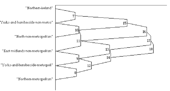
Example:

$$X=\left[\begin{array}[]{ccccc}[1,4]&2&(1(0.4),2(0.1),3(0.2),4(0.07),5(0.02))&(1(0.1),2(0.9))&(1(0.7),2(0.2))\\ [1,4]&3&(1(0.6),2(0.1),3(0.1),5(0.0))&(1(0.1),2(0.9))&(1(0.7),2(0.2))\\ [1,5]&2&(1(0.7),2(0.2))&(1(0.0),2(0.9))&(1(0.7),2(0.2))\\ [1,4]&1&(1(0.7),2(0.0),3(0.1),4(0.0),5(0.0),6(0.0),7(0.0))&(1(0.0),2(0.9))&(1(0.7),2(0.2))\\ [1,4]&1&(1(0.4),3(0.4),4(0.0),5(0.0))&(1(0.0),2(0.9))&(1(0.8),2(0.1))\\ [1,6]&2&(2(0.4),3(0.1),4(0.3),5(0.0),6(0.0),7(0.0))&(1(0.0),2(0.9))&(1(0.7),2(0.2))\end{array}\right]$$
Refer to caption
Figure 1: Pyramid produced using CAPS

The algorith CAPS, with the matrix $X$ as input, produces the pyramid of the Figure 1, and if we use the algorithm CAPSO with the order 8, 6, 4, 2, 5, 3, 1 given a priori, then we get the pyramid of the Figure 2.

Where the symbolic objects asociated to each node and their extension of the pyramid presented Figure 1 are:

P7=[y1=[1.000,4.000]]^[y2={1.00}]^[y3=(1(0.7181),2(0.0537),3(0.4348),
Ψ4(0.0870),5(0.0435),6(0.0134),7(0.0067))]^[y4=(1(0.0435),2(0.9799
Ψ))]^[y5=(1(0.8696),2(0.2483))]
Ext(P7)={4,5}
P8=[y1=[1.000,5.000]]^[y2={2.00}]^[y3=(1(0.7882),2(0.1151),3(0.2806),
Ψ4(0.0791),5(0.0288),6(0.0000),7(0.0000))]^[y4=(1(0.0588),2(0.9856)
Ψ)]^[y5=(1(0.7765),2(0.2734))]
Ext(P8)={1,3}
etc....
Refer to caption
Figure 2: Pyramid produced by CAPSO

References

  • [1] Bertrand P. Etude de la representation pyramidale, Thèse de 3 cycle, Universite Paris IX-Dauphine, 1986.
  • [2] Bertrand P et Diday E. Une generalisation des arbres hierarchiques: Les representations pyramidales, Statistique Appliquee, (3), 53-78, 1990.
  • [3] Brito P. Analyse de donnees symboliques: Pyramides d’heritage, Thèse de doctorat, Universite Paris 9 Dauphine, 1991.
  • [4] Brito P. Symbolic clustering of probabilistic data, Adavances in Data Science and Classification, eds. Rizzi A., Vichi M. and Bock H., Springer-Verlag, pp385-390, 1998.
  • [5] Diday E. Une representation visuelle des classes empietantes. Rapport INRIA n. 291. Rocquencourt 78150, France, 1984.
  • [6] Diday E., Lemaire J., Pouget J., Testu F. Elements d’Analyse des donnees. Dunod, Paris, 1984.
  • [7] Diday E. Introduction l’approche symbolique en Analyse des Donnes. Proc. Première Journees Symbolique-Numerique. Universite Paris IX Dauphine. Decembre 1987.
  • [8] Diday E. L’Analyse des Donnes Symboliques: un cadre theorique et des outils. Cahiers du CEREMADE, 1998.
  • [9] Diday E., and Bock H–H. (eds.). Analysis of Symbolic Data. Exploratory methods for extracting statistical information from complex data. Springer Verlag, Heidelberg, 425 pages, ISBN 3-540-66619-2, 2000.
  • [10] Gil A., Capdevila C. and Arcas A. On the efficiency and sensitivity of a pyramidal classification algorithm, Economics working paper 270, Barcelona, 1998.
  • [11] Mfoumoune E. Les aspects algorithmiques de la classification ascendante pyramidale et incrementale. Thèse de doctorat, Universite Paris 9 Dauphine, 1998.
  • [12] Pollaillon G. Organisation et interpretation par les treillis de Galois de donnees de type multivalue, intervalle ou histogramme. These de doctorat, Universite Paris 9 Dauphine, 1998.