INTERSTATIS: The STATIS method for interval valued data

E

Abstract

The STATIS method, proposed by L’Hermier des Plantes and Escoufier, is used to analyze multiple data tables in which is very common that each of the tables have information concerning the same set of individuals. The differences and similitudes between said tables are analyzed by means of a structure called the compromise. In this paper we present a new algorithm for applying the STATIS method when the input consists of interval data. This proposal is based on Moore’s interval arithmetic and the Centers Method for Principal Component Analysis with interval data, proposed by Cazes el al. [5]. In addition to presenting the INTERSTATIS method in an algorithmic way, an execution example is shown, alongside the interpretation of its results.

l método STATIS, propuesto por L’Hermier des Plantes y Escoufier, se utiliza para analizar múltiples tablas de datos en las cuales es muy frecuente que cada una de la tablas tenga información referente al mismo conjunto de individuos. Las diferencias y similitudes entre dichas tablas se analizan por medio de una estructura llamada compromiso. En este trabajo se presenta un nuevo algoritmo, denominado INTERSTATIS, del método STATIS para el caso cuando los datos de entrada son todos de tipo intervalo. Esta propuesta se basa en la aritmética de intervalos de Moore y el Método de Centros para el Análisis de Componentes Principales con datos de tipo intervalo, propuesto por Cazes et al. [5]. Además de presentar el método INTERSTATIS de forma algorítmica, un ejemplo de ejecución es presentado, junto con la interpretación de sus resultados.

INTERSTATIS, STATIS, Aritmética de intervalos, datos tipo intervalo, Análisis de datos simbólico.

INTERSTATIS, STATIS, Interval Arithmetic, Interval Data, Symbolic data analysis.

Mathematics Subject Classification: 62-07.

1 Introduction

Given the flexibility and various applications of the Principal Component Analysis (PCA), L’Hermier des Plantes [12] and Escoufier [7, 10] worked, sequentially, in a generalized version of the method, to study multiple data tables. The method, named STATIS, is capable of analyzing several groups of tables, referring to the same variables or the same individuals (STATIS DUAL). The STATIS uses the PCA as part of the necessary transformations to reach a structure called the compromise, used in evaluating the differences and similitudes amongst the input tables.

Taking into account the potential of the STATIS, as an 3-index information analysis tool, the initiative of extending the method to the case of interval symbolic objects [3, 13, 2, 6] was born. These objects are meant to represent second order inviduals, whose given concepts are much more complex than simple points in $\mathbb{R}^{n}$. For example, interval vectors, histograms, graphs, trees, rules, sets, functions, etc.

Although there already exist works in the field of symbolic methods for data analysis, like the generalizations of the Principal Components Analysis (PCA) [5, 9, 15] and the $k$-means [19] among others, the STATIS method has not been reformulated to handle symbolic objects. The first step consists in finding a way to generalize the STATIS, while guaranteeing that the classic method is an specific case of the symbolic proposal. This restriction is important since it ensures that the proposal has a sound statistical meaning.

Initially, Moore’s Interval Arithmetic (IA) [4, 14] was proposed to perform operations between intervals. This arithmetic was created to handle, in a bounded way, the uncertainty in operations amongst non-exact quantities, and thus, provides a natural transition for the elemental operations –addition, substraction, division and multiplication– from the classic case to the symbolic one. Besides, it is simple in its definition, implementation and complies with the fact that the operations between real numbers are specific cases of the IA, making it a good starting point for the generalization of the STATIS.

Additionally, knowing that the PCA is an integral part of the STATIS, it was necessary to have a PCA variant capable of handling interval valued data. To solve this need the Centers PCA (CPCA) by Cazes et al. [5] was used. This PCA gives as a result a representative hypercube for each individual, where its variation (in width, depth and height) describes the correspondent individual’s variation.

Besides the regular interval notation, the $\widehat{\times}$ notation is used to indicate interval arithmethic operations. In the case of the dot product between symbolic matrices, its definition is analog to the dot product between real matrices, but using the IA multiplication.

Note as well the use of boldface to denote interval valued variables. For example, $\mathbf{X}$ denotes an interval matrix, while $X$ stands for a classic matrix. This provision facilitates distinguishing between both cases throughout the paper.

2 INTERSTATIS with IA and Centers PCA

This first version of the INTERSTATIS for interval data, works by replacing the conventional –or classic– operations, with their IA counterparts. Also, the CPCA, with its interval inputs and outputs, replaces the classic PCA method.

During the preprocessing phase of the input matrices, it is a requisite to center them. For this step the Rodríguez [16] intervals mean was used. It follows:

Definición 1 (Intervals Mean)

Let $\mathbf{Y}$ be an interval valued variable, defined over $E=\{1,2,\ldots,n\}$ for $\mathbf{Y}=\{[\underline{y}_{1},\overline{y}_{1}]\,[\underline{y}_{2},\overline{y}_{2}],\ldots,[\underline{y}_{n},\overline{y}_{n}]\}$, the mean is defined as:

$$\overline{\mathbf{Y}}=\left[\frac{1}{n}\sum_{i=1}^{n}\underline{y}_{i},\frac{1}{n}\sum_{i=1}^{n}\overline{y}_{i}\right]\text{.}$$

Following, the INTERSTATIS algorithm using IA and CPCA, as a generalization of the version presented by González and Rodríguez in [8].

 

INTERSTATIS with AI and CPCA

Input: $r$ data tables (matrices) $\mathbf{X}_{k}\in\mathcal{I}(\mathbb{M}^{n\times p_{k}})$ individuals$\times$variables of size $n\times p_{k}$, centered with respect to $D$ (using Definition 1 for the means), where

• $n$ is the number of individuals, the same in the $r$ measurings.

• $p_{k}$ is the number of variables in the $k$th measuring.

• $D=diag(1/n,1/n,\ldots,1/n)$ is the weights matrix, invariant for the $r$ measurings.

• $l=\sum_{k=1}^{r}p_{k}$ is the amount of variables in all tables.

Output: the following tables are generated:

• $\mathbf{T}\in\mathcal{I}(\mathbb{M}^{r\times r})$ with the correlations between tables (step 4).

• $\mathbf{E_{v}}\in\mathcal{I}(\mathbb{M}^{l\times l})$ with the evolution of the variables (step 7).

• $\mathbf{M_{i}}\in\mathcal{I}(\mathbb{M}^{n\times l})$ with the average individuals (step 7).

• $\mathbf{E_{i}}\in\mathcal{I}(\mathbb{M}^{rn\times l})$ with the evolution of the individuals (step 11).

Interstructure: (steps 1-4). Given that the individuals in the $r$ measurings are the same, it is possible to compare their spatial distribution by means of the $\mathbf{W}_{i}=\mathbf{X}_{i}\widehat{\times}\mathbf{X}_{i}^{T}$ matrices. For this, the metric defined by the internal product is used

$$<\mathbf{W}_{i},\mathbf{W}_{j}>_{\phi}=trace(\mathbf{W}_{i}\widehat{\times}\mathbf{W}_{j})=<\vec{\mathbf{W}_{i}}\widehat{\times}\vec{\mathbf{W}_{j}}>_{I}$$

where $\vec{\mathbf{W}_{i}}\in\mathcal{I}(\mathbb{R}^{n^{2}})$ is the vector formed by all the rows of the $\mathbf{W}_{i}$ matrix, for $i=1,2,\ldots,r$.

• Step 1: Compute the $\mathbf{W}_{i}\in\mathcal{I}(\mathbb{M}^{n\times n})$ matrices, given by $\mathbf{W}_{i}=\mathbf{X}_{i}\widehat{\times}\mathbf{X}_{i}^{T}$ for $i=1,2,\ldots,r$.

• Step 2: Generate the following matrix

  $$\mathbf{X}=\left[\ \vec{\mathbf{W}_{1}}\ |\ \vec{\mathbf{W}_{2}}\ |\ \cdots|\ \vec{\mathbf{W}_{r}}\ \right]_{\mathcal{I}(n^{2}\times r)}$$

• Step 3: Perform a CPCA for the triplet $(\mathbf{X},D_{\frac{1}{\sigma^{2}}},\frac{1}{n^{2}}I_{n}^{2})$.

  Store the resulting principal components as

  $$\mathbf{T}=\left[\mathbf{PC}_{1},\mathbf{PC}_{2},\ldots,\mathbf{PC}_{r}\right]_{\mathcal{I}(r\times r)}\text{.}$$

  Also store the first eigenvector, noted by $u=(u_{1},u_{2},\ldots,u_{r})$, and the first eigenvalue $\lambda_{1}$, both real, to use them later on in the creation of the compromise. It is not necessary to convert these to interval data since the IA defines operations between interval and real values.

• Step 4: Plot the correlations circle from the $\mathbf{T}$ matrix. Each point represents a data table, where close points mean similar individual configurations, and parallel vectors represent homothetic configurations.

Intrastructure: (steps 5-12). The evolutive study of the individuals and the variables is performed through the compromise $\sum_{k=1}^{r}\mathbf{\beta}_{k}\mathbf{W}_{k}$ product of the CPCA with parameters $(\mathbf{\tilde{X}},I_{l},D)$, where $\mathbf{\beta}_{k}$ is defined in step 5 and $\mathbf{\tilde{X}}$ is defined as:

$$\mathbf{\tilde{X}}=\left[\ \mathbf{\beta}_{1}\widehat{\times}\mathbf{X}_{1}\ |\ \mathbf{\beta}_{2}\widehat{\times}\mathbf{X}_{2}\ |\ \cdots|\ \mathbf{\beta}_{r}\widehat{\times}\mathbf{X}_{l}\right]_{\mathcal{I}(n\times l)}$$

• Evolution of the variables: (steps 5-9)

  • Step 5: Compute $\mathbf{\beta}=(\mathbf{\beta}_{1},\mathbf{\beta}_{2},\ldots,\mathbf{\beta}_{r})=\frac{1}{\sqrt{\lambda_{1}}}u$.

  • Step 6: Compute the blocks matrix $\mathbf{\tilde{X}}$ as follows:

    $$\mathbf{\tilde{X}}=\left[\ \mathbf{\beta}_{1}\widehat{\times}\mathbf{X}_{1}\ |\ \mathbf{\beta}_{2}\widehat{\times}\mathbf{X}_{2}\ |\ \cdots|\ \mathbf{\beta}_{r}\widehat{\times}\mathbf{X}_{l}\right]_{\mathcal{I}(n\times l)}$$

  • Step 7: Perform a CPCA for ($\mathbf{\tilde{X}},I_{l},D$). Store the principal components $\mathbf{M_{i}}$ and the principal correlations $\mathbf{E_{v}}$, in the following way

    $$\mathbf{M_{i}}=\left[\mathbf{C}_{1},\mathbf{C}_{2},\ldots,\mathbf{C}_{l}\right]_{\mathcal{I}(n\times l)}\text{\quad y\quad}\mathbf{E_{v}}=\left[\mathbf{PC}_{1},\mathbf{PC}_{2},\ldots,\mathbf{PC}_{n}\right]_{\mathcal{I}(l\times l)}\text{.}$$

  • Step 8: Plot the correlations circle from $\mathbf{E_{v}}$, in which it is possible to study the evolution of the variables.

  • Step 9: Plot the principal plane based on $\mathbf{M_{i}}$, in which the $n$ average individuals (see definition in [11]) are represented.

• Evolution of the individuals: (steps 10-12)

  • Step 10: Compute the IND matrix, defined by blocks as:

    $$\texttt{IND}=\left[\begin{array}[]{c}\mathbf{W}_{1}\\ \mathbf{W}_{2}\\ \vdots\\ \mathbf{W}_{r}\\ \end{array}\right]_{\mathcal{I}(rn\times n)}$$

  • Step 11: Compute the coordinates for the individuals throughout the different tables, noted as $\mathbf{E_{i}}$, through the following matrix product:

    $$\mathbf{E_{i}}=\texttt{IND}\widehat{\times}\mathbf{M_{i}}$$

  • Step 12: Plot the principal plane using $\mathbf{E_{i}}$. In this chart, one can study the evolution of the individuals.

 

The following results prove that the classical STATIS is a particular case of the INTERSTATIS with IA and CPCA.

Definición 2 (Classical and interval matrix equivalence)

Let $X\in\mathbb{M}^{n\times p}$ and $\mathbf{Y}\in\mathcal{I}(\mathbb{M}^{n\times p})$. Then, $X$ is matrix-equivalent to $\mathbf{Y}$, noted by $X\equiv\mathbf{Y}$ if

$$X\equiv\mathbf{Y}\iff\forall\ x_{ij}\in X,\forall\ \mathbf{y}_{ij}\in\mathbf{Y}:x_{ij}=\underline{\mathbf{y}_{ij}}=\overline{\mathbf{y}_{ij}}$$

with $i=\{1,2,\ldots,n\}$ and $j=\{1,2,\ldots,p\}$.

Lema 1

The classic PCA is a particular case of the CPCA [16].

Lema 2

The classic operations $\{+,-,\times,/,\sqrt{\cdot}\}$ are particular cases of the IA [14].

Teorema 1

The classic STATIS is a particular case of the INTERSTATIS with IA and CPCA.

Due to space concerns the proof has been ommitted, although it is trivial.

Corolario 1

Let $X\in\mathbb{M}^{n\times p}$ and $\mathbf{Y}\in\mathcal{I}(\mathbb{M}^{n\times p})$ with $X\equiv\mathbf{Y}$, then the output of the STATIS taking $X$ as input, is the same as the INTERSTATIS output, taking $\mathbf{Y}$ as input.

3 Experiments

This section is concerned with the data used in the tests and the interpretation of the correspondent results.

For the experiments a data table based on the wine data by Abdi [1] was generated. This table describes the criteria from three different wine experts, on six different types of wines, depending on the type of oak barrels used in their aging process. For each wine sample, the intensity of a given flavor is defined in a scale from 1 to 10. Also, for the generated table, the center of each one of its entries is the same as the correspondent entry in the original data table. Mathematically, let $X$ be the classic wines table and $\mathbf{Y}$ the test data matrix, then

$$\forall\ x_{ij}\in X,\forall\ \mathbf{y}_{ij}\in\mathbf{Y}:x_{ij}=m(\mathbf{y}_{ij}),$$

with $i=\{1,2,\ldots,n\}$, $j=\{1,2,\ldots,p\}$ and where $m(\mathbf{y})$ is the middle point or center of the interval $\mathbf{y}$.

This property for the test table is based on the way the CPCA works. This method projects, for each interval, the center and then the minima and maxima in supplementary. Therefore, if the center –for each entry– of the test table is equal to the value in the original table, the individuals will have a similar spatial placement in the experiment.

3.1 Interpretation of the results

Each of the figures presents the output of the INTERSTATIS using the test table, with the first two axes used for plotting. The charts in this paper were generated in Mathematica.

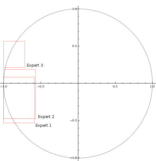
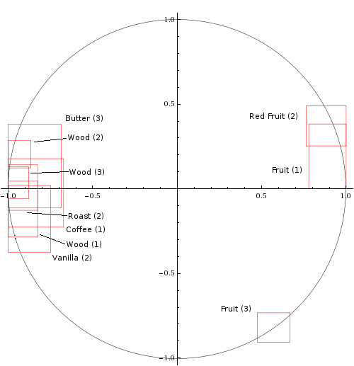
(a) Correlations amongst tables	(b) Evolution of the variables
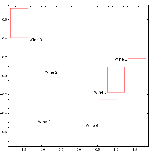
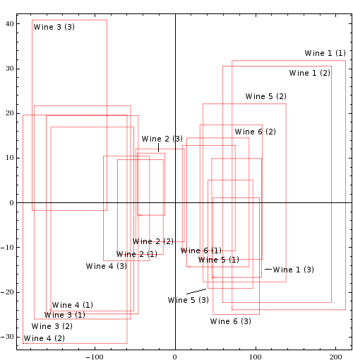
(c) Average individuals	(d) Evolution of the individuals

Figure 1: Output of the INTERSTATIS method.

Analyzing figure 1a, the test data produces a very similar output to that of the STATIS, given that experts 1 and 2 are correlated given their similitude, leaving expert 3 on its own. Nonetheless, the distance between the groups of tables is variable, as a consequence of the use of interval data. For example, the closeness of the borders for experts 2 and 3 indicates a similar behavior in said borders, nonexistent in the classic case. It is precisely this capability of handling a level of uncertainty, the advantage of this symbolic proposal, since it analyzes not only the variation amongst individuals, but their internal variation as well.

Figure 1b presents a very similar correlations structure in comparison to the one generated by the STATIS, showing three groupings of variables, but in the symbolic case overlapping occurs amongst said groups. It should be noted that the representations for the variables in 1b are near the borders of the circle, clear sign of marked correlations. If follows that results drawn upon them are thus valid.

In the average individuals plane (figure 1c) the additional information provided by the INTERSTATIS can be appreciated, through the size of the rectangles, given that their size is proportionate to the average size of the represented individual.

In the last step (figure 1d) the evolution of the individuals is studied, that is, their changes throughout all the tables or measurings. Given the amount of rectangles present ($r\times n$), this plane should ideally be plotted using a subset of the individuals, to aid in its interpretation. For example, visualize the evolution of a pair of individuals to better appreciate their variation and interaction.

It is important to remark that the symbolic proposal adds analysis information without sacrificing that already provided by the classic method, that is, produces more information by the use of intervals. Nevertheless, the interpretation complexity is increased as well. For this proposal, an aspect that heavily affects the output of the method is the width of the input intervals and therefore, the input tables should be normalized so that the width of its elements is reduced and the output remains useful.

Another relevant characteristic of symbolic analysis, which adds value to the proposal, lies in its ability to reveal possible interactions between individuals or variables, hidden in the results obtained through the classic methods.

4 Conclusions and future work

A new proposal for applying the STATIS method when the input data consists of interval valued data was proposed. This proposal permits the method to handle internal variation in the input data, therefore allowing the use of representations which better reflect the true nature of that which is measured. It was also proved that the STATIS is a particular case of the proposed INTERSTATIS with IA and CPCA, thus validating its statistical usefulness.

Another important benefit resides in the use of symbolic objects per se, given that they can be used to compact copious amounts of data, while minimizing data loss during the process. Once these symbolic objects are created, the INTERSTATIS –as well as any other symbolic method– allows the exploration and analysis of the totality (or a majority) of the individuals present in the original data table.

With regards to future work, although the obtained results have been positive, there exist other interval arithmetics (and modifications of these) that could help make the output of the INTERSTATIS more compact. Finally, a generalization of the STATIS method to treat histogram valued data is an open problem.

References

- [1] Abdi, H. & Valentin, D. (2006) “The STATIS Method”, Encyclopedia of Measurement and Statistics. Volume 2.
- [2] Billard, L. & Diday, E. (2006) Symbolic Data Analysis: Conceptual Statistics and Data Mining, John Wiley & Sons Ltd, United Kingdom.
- [3] Billard L., Douzal-Chouakria A. and Diday E. (2011) “Symbolic Principal Components For Interval-Valued Observations”, Statistical Analysis and Data Mining. 4 (2), 229-246. Wiley.
- [4] Caprani, O., Madsen, K., Nielsen, H. (2002) “Introduction to Interval Analysis”, Informatics and Mathematical Modelling, Technical University of Denmark, DTU, pp. 82.
- [5] Cazes P., Chouakria A., Diday E. et Schektman Y. (1997) “Extension de l’analyse en composantes principales à des données de type intervalle”, Rev. Statistique Appliquée, Vol. XLV Num. 3 pag. 5-24, France.
- [6] Diday E. (1987): “Introduction à l’approche symbolique en Analyse des Données”. Premières Journées Symbolique-Numérique. Université Paris IX Dauphine. Paris, France.
- [7] Escoufier, Y. (1980) L’analyse conjointe de plusieurs matrices de données. In M. Jolivet (Ed.), Biométrie et Temps. Paris: Société Française de Biométrie. pp. 59-76.
- [8] González, J. & Rodríguez, O. (1995) “Algoritmo e Implementación del método STATIS”, IX Simposio Métodos Matemáticos Aplicados a las Ciencias, J.Trejos (ed.), UCR-ITCR, Turrialba.
- [9] Lauro, C. & Palumbo F. (2001) “Principal Component Analysis of Interval Data: a Symbolic Data Analysis Approach”. Computational Statistics, Vol. 15 n.1, pp. 73-87.
- [10] Lavit, Ch., Escoufier Y., Sabatier, R., & Traissac, P., (1994) “The ACT (STATIS) method”. Computational Statistics & Data Analysis, 18, pp. 97-119.
- [11] Lavit, Ch., (1988) Analyse Conjointe de Tableaux Quantitatifs, Ed. Masson, París.
- [12] L’Hermier des Plantes, H. (1976) Structuration des tableaux à trois indices de la statistique. Thèse de troisième cycle. Universitè de Montpellier, Montpellier, France.
- [13] Makosso-Kallyth S. and Diday E. (2012) “Adaptation of interval PCA to symbolic histogram variables”, Advances in Data Analysis and Classification July, Volume 6, Issue 2, pp 147-159.
- [14] Moore, R.E. (1979) “Methods and Applications of Interval Analysis”, Society for Industrial and Applied Mathematics (SIAM), Philadelphia, USA.
- [15] Rodríguez, O., Diday E., Winsberg S. (2001) “Generalization of the Principal Component Analysis to Histogram Data”. Workshop on Simbolic Data Analysis of the 4th European Conference on Principles and Practice of Knowledge Discovery in Data Bases, Setiembre 12-16, 2000, Lyon, France.
- [16] Rodríguez, O. (2000) Classification et Modèles Linéaires en Analyse des Doneés Symboliques. Thèse de doctorat, Université Paris IX Dauphine, Paris, France.
- [17] Stolfi, J. & de Figueiredo, L. (2003) “An Introduction to Affine Arithmetic”, TEMA Tend. Mat. Apl. Comput., 4, Vol.3, pp. 297-312.
- [18] Stolfi, J. & de Figueiredo, L. (1997) “Self-Validated Numerical Methods and Applications”, Brazilian Mathematics Colloquium monograph, IMPA, Rio de Janeiro, Brasil.
- [19] Verde, R., De Carvalho, F.A.T., LeChevallier, Y. (2000) “A Dynamical Clustering Algorithm for Multi-Nominal Data”. In : H.A.L. Kiers, J.-P. Rasson, P.J.F. Groenen and M. Schader (Eds.): Data Analysis, Classification, and Related Methods, Springer-Verlag, Heidelberg, 387-394.