Multidimensional Scaling for Interval Data: INTERSCAL

Abstract

Standard multidimensional scaling takes as input a dissimilarity matrix of general term $\delta_{ij}$ which is a numerical value. In this paper we input $\delta_{ij}=[\underline{\delta_{ij}},\overline{\delta_{ij}}]$ where $\underline{\delta_{ij}}$ and $\overline{\delta_{ij}}$ are the lower bound and the upper bound of the “dissimilarity” between the stimulus/object $S_{i}$ and the stimulus/object $S_{j}$ respectively. As output instead of representing each stimulus/object on a factorial plane by a point, as in other multidimensional scaling methods, in the proposed method each stimulus/object is visualized by a rectangle, in order to represent dissimilarity variation. We generalize the classical scaling method looking for a method that produces results similar to those obtained by Tops Principal Components Analysis. Two examples are presented to illustrate the effectiveness of the proposed method.

S. Winsberg, O. Rodríguez and E. Diday LISE–CEREMADE, Université de Paris IX Dauphine. LISE–CEREMADE, Université de Paris IX Dauphine. IRCAM, 1 Place Igor Stravinsky, F–75004, Paris, France.

Keywords

Symbolic object, multidimensional scaling, interval data, dissimilarity variation.

1 Introduction

Let $S_{1},S_{2},\ldots,S_{m}$ be $m$ stimuli/objects, we assume that the data consist of a symmetric matrix $\Delta=([\delta_{ij}])=[\underline{\delta_{ij}},\overline{\delta_{ij}}]$, $i,j=1,2,\ldots,m$ where $[\underline{\delta_{ij}},\overline{\delta_{ij}}]$ represents the lower and upper limits respectively of the set of the possible values for the dissimilarity between the stimulus/object $S_{i}$ and the stimulus/object $S_{j}$. The set of possible values for the dissimilarity between the stimulus/object $S_{i}$ and the stimulus/object $S_{j}$ might result from combining data from $N$ judges or sources, or alternatively it might be a region of dissimilarity proposed by a single judge/source. Of course, the interval of dissimilarities for each pair of stimuli/objects could be trimmed on each end by five percent of the values, or the inter–quartile range could be used instead of the entire interval. So instead of a data table of dissimaliarities, that is a table of numerical values for the dissimilarity of each stimulus/object pair, we have a data table consisting of intervals representing the lower and upper limits of dissimilarity for each stimulus/object pair.

Consider a set of stimuli consisting of rectangles of varying area, ie size, and height–to–width ratio, ie shape, presented pairwise to subjects on a computer screeen. The subjects respond to each pair with a dissimilarity judgment. The dissimilarity between stimulus $i$ and stimulus $j$ can be represented as an interval, since each all the judges may not respond in the same way. Therefore, each “psychological”, or “perceptual”, rectangle is not precisely located, even though the corresponding “physical” rectangle occupies a point in two–dimensional space. Moreover, the dimensions used to make the disssimilarity judgments might be size and shape, or height and width, or something else. In fact an aim of multidimensional scaling, MDS, is to locate the stimuli–objects in a low–dimensional space, and interpret the dimensions giving rise to the dissimilarity judgments. With our approach we will also determine how well each stimulus/object is localized.

We have chosen to represent the objects $S_{i}$ and $S_{j}$ as hypercubes in a low–dimensional Euclidean space, rather than say for example hyperspheres because the hypercube representation is reflected as a conjunction of $n$ properties, where $n$ is the dimensionality of the space. This representation as a conjunction is appealing for two reasons. The first reason is linguistic. In everyday language one refers to rectangles having both an area lying between 10 and 20 square centimters, and a height–to–width ratio lying between 0.5 and 0.8; one does not refer to a rectangle with an area and shape centered at 15 square centimeters and 0.65 with a radius of 0.75, the radius to be expressed in just what units. In fact when one queries a data base, the query is expressed as a conjunction. The second reason is that this representation as a conjunction fits within a data analytic framework concerning symbolic objects. This data analytic framework has proved to be useful in dealing with large data bases.

A symbolic object is a model for an entity which can be an individual or a concept of the real world equipped with a means of comparing the description of this entity to the description of an individual observation. More precisely, it is defined by: $i)$ a description $D$, say area $[10,20]$ and height–to–width ratio $[0.5,0.8]$; $ii)$ a binary relation $R$, say $=$, $\leq$, or $\in$, permitting the comparison between two descriptions to the entire set of descriptions $\cal D$; $iii)$ a function, or mapping, $a$ providing a means of evaluating the result of the comparison (using $R$) of the description of an individual in $\Omega$ the set of all the individuals to the descripton $D$. The extent of a symbolic object $a$ is the set of individuals who fit the description. Thus, a symbolic object is defined by the triple $s=(a,R,D)$ where $a$ depends on the relation $R$ and the description $D$. Interval data are a type of symbolic data, so we might have for example, $a(w)=[size(w)\in[10,20]]\wedge[shape(w)\in[0.5,0.8]]$ defining a symbolic object $s=(a,R,D)$.

The representation of the upper and lower values for the distance between symbolic object $S_{i}$ and symbolic object $S_{j}$ is given in equations (1) and (2), below.

Let be $R_{S_{i}}$ the hypercube defined in ${\mbox{$IR$}}^{n}$ by the symbolic object $S_{i}$, $R_{S_{j}}$ the hypercube in ${\mbox{$IR$}}^{n}$ defined by the symbolic object $S_{j}$ and let $\underline{d_{ij}}$ end $\overline{d_{ij}}$ the minimum and the maximum Euclidean distances between $R_{S_{i}}$ and $R_{S_{j}}$. Then (where $\underline{x_{ik}}$ and $\overline{x_{jk}}$ are defined in the equation (3) below) one could be represent $\overline{d_{ij}}$ and $\underline{d_{ij}}$ as:

$$\overline{d_{ij}}=\frac{1}{2}\sqrt{\sum\limits_{k=1}^{n}\left[\left(\overline{x_{ik}}-\underline{x_{ik}}\right)+\left(\overline{x_{jk}}-\underline{x_{jk}}\right)+2\left|\frac{\overline{x_{ik}}-\underline{x_{ik}}}{2}-\frac{\overline{x_{jk}}-\underline{x_{jk}}}{2}\right|\right]^{2}}$$ (1)

$$\underline{d_{ij}}=\frac{1}{4}\sqrt{\left[\sum\limits_{k=1}^{n}\left(\overline{x_{ik}}-\underline{x_{ik}}\right)+\left(\overline{x_{jk}}-\underline{x_{jk}}\right)-2\left|\frac{\overline{x_{ik}}-\underline{x_{ik}}}{2}-\frac{\overline{x_{jk}}-\underline{x_{jk}}}{2}\right|-\sim\right.}$$

$$\overline{\left.\sim\left|\left(\overline{x_{ik}}-\underline{x_{ik}}\right)+\left(\overline{x_{jk}}-\underline{x_{jk}}\right)-2\left|\frac{\overline{x_{ik}}-\underline{x_{ik}}}{2}-\frac{\overline{x_{jk}}-\underline{x_{jk}}}{2}\right|\right|\right]^{2}}$$ (2)

Denœux and Masson (1999) have proposed a solution to this problem minimizing the stress function, $\sigma(\mathcal{R})$, by gradient descent:

$$\sigma(\mathcal{R})=\sum\limits_{i<j}(\underline{d_{ij}}-\underline{\delta_{ij}})^{2}+\sum\limits_{i<j}(\overline{d_{ij}}-\overline{\delta_{ij}})^{2},$$

where $\underline{d_{ij}}$ and $\overline{d_{ij}}$ represent, respectively, the minimum and the maximum Euclidean distances between of the region $R_{i}$ and $R_{j}$ that they are looking for in ${\mbox{$IR$}}^{p}$ to represent the symbolic object $S_{i}$ and $S_{j}$ respectively. Their approach has two problems. First it could find a local minimum. Second the minimization by gradient descent is not optimal and the computation of the gradient of their stress function is difficult to implement.

To avoid these problems we propose a method for multidimensional scaling of interval data, INTERSCAL, with a different approach. We generalize the classical scaling method of Torgenson (1958) and Gower (1966) by looking for a method that produces results similar to the Tops Method in Principal Component Analysis proposed by (Cazes, Chouakria, Diday and Schektman (1997)). The Tops Method extends standard principal component analysis to interval data. Standard principal component analysis, as a dimensional reduction method, aims at reducing the number of descriptive features while taking into account the main structure of the data. In the Tops Method, similarly, the aim is to reduce the number of interval features, called interval principal components. The variability or the inaccuracy of the descriptive features are expressed, after the reduction, by interval principal components and visualized by rectangles in the factorial space.

2 Multidimensional scaling for interval data

In the Tops Method case the input are $m$ symbolic objects $S_{1},S_{2},\ldots,S_{m}$ described by $n$ interval variables $X^{1},X^{2},\ldots,X^{n}$ like we show in equation (3).

$$\left(\begin{array}[]{c}S_{1}\\ \vdots\\ S_{m}\end{array}\right)=\left(\begin{array}[]{ccc}X_{S_{1}1}&\cdots&X_{S_{1}n}\\ \vdots&\ddots&\vdots\\ X_{S_{m}1}&\cdots&X_{S_{m}n}\end{array}\right)=\left(\begin{array}[]{ccc}\left[\underline{x_{11}},\overline{x_{11}}\right]&\cdots&\left[\underline{x_{1n}},\overline{x_{1n}}\right]\\ \vdots&\ddots&\vdots\\ \left[\underline{x_{m1}},\overline{x_{m1}}\right]&\cdots&\left[\underline{x_{mn}},\overline{x_{mn}}\right]\end{array}\right)$$ (3)

With this matrix we construct a new numerical matrix $M$ of $2^{m}\cdot n$ rows and $n$ columns as we show in the equation (3); then the Tops Method applies the standard Principal Component Analysis method to the matrix $M$.

$$M=\left[\begin{array}[]{c}\left[\begin{array}[]{cccc}\underline{x_{11}}&\underline{x_{12}}&\cdots&\underline{x_{1n}}\\ \underline{x_{11}}&\underline{x_{12}}&\cdots&\overline{x_{1n}}\\ \vdots&\vdots&\ddots&\vdots\\ \overline{x_{11}}&\overline{x_{12}}&\cdots&\overline{x_{1n}}\end{array}\right]\\ \left[\begin{array}[]{cccc}\underline{x_{21}}&\underline{x_{22}}&\cdots&\underline{x_{2n}}\\ \underline{x_{21}}&\underline{x_{22}}&\cdots&\overline{x_{2n}}\\ \vdots&\vdots&\ddots&\vdots\\ \overline{x_{21}}&\overline{x_{22}}&\cdots&\overline{x_{2n}}\end{array}\right]\\ \vdots\\ \left[\begin{array}[]{cccc}\underline{x_{m1}}&\underline{x_{m2}}&\cdots&\underline{x_{mn}}\\ \underline{x_{m1}}&\underline{x_{m2}}&\cdots&\overline{x_{mn}}\\ \vdots&\vdots&\ddots&\vdots\\ \overline{x_{m1}}&\overline{x_{m2}}&\cdots&\overline{x_{mn}}\end{array}\right]\end{array}\right],$$ (4)

Let $S_{1},S_{2},\ldots,S_{m}$ be $m$ symbolic objects, we assume that the input data consists of a symmetric matrix $\Delta$ defined by:

$$\Delta=\left[\begin{array}[]{cccc}[\underline{\delta_{11}},\overline{\delta_{11}}]&[\underline{\delta_{12}},\overline{\delta_{12}}]&\cdots&[\underline{\delta_{1m}},\overline{\delta_{1m}}]\\ [\underline{\delta_{21}},\overline{\delta_{21}}]&[\underline{\delta_{22}},\overline{\delta_{22}}]&\cdots&[\underline{\delta_{2m}},\overline{\delta_{2m}}]\\ \vdots&\vdots&\ddots&\vdots\\ [\underline{\delta_{m1}},\overline{\delta_{m1}}]&[\underline{\delta_{m2}},\overline{\delta_{m2}}]&\cdots&[\underline{\delta_{mm}},\overline{\delta_{mm}}]\end{array}\right],$$ (5)

where $\underline{\delta_{ij}}$ represents the lower bound of the dissimilarity between the symbolic object $S_{i}$ and the symbolic object $S_{j}$ and $\overline{\delta_{ij}}$ represents the upper bound of the dissimilarity between the symbolic object $S_{i}$ and the symbolic object $S_{j}$.

It is well known that there is a duality property between principal components analysis and classical multidimensional scaling where the dissimilarities are given by Euclidean distances. Formally, if $\mu_{i}$ and $\xi_{i}$ are the eigenvalues and eigenvectors of the principal components analysis respectively for $i=1,2,\ldots,n$, and we denote by $\lambda_{i}$ and $v_{i}$ the eigenvalues and eigenvectors of the multidimensional scaling respectively for $i=1,2,\ldots,n$ then $\mu_{i}=\lambda_{i}$ and $\xi_{i}=X^{t}v_{i}$ for $i=1,2,\ldots,n$.

If we want to get a Symbolic Multidimensional Scaling method that has the duality property with the Tops Principal Components Analysis method, when dissimilarity is modeled by an Euclidean distance, we need as input the dissimilarities between all the rows of the matrix $M$ defined in (4), because the Tops Principal Component Analysis method starts by doing a classical principal component analysis of the matrix $M$ defined in (4).

Since the size of $M$ has $m\cdot 2^{n}$ rows and $n$ columns, we should have as input a matrix $\Delta$ of size $m\cdot 2^{n}\times m\cdot 2^{n}$ but this is clearly impossible, because we only have two dissimilarities, that is the maximun and the minimum, for each pair of symbolic objects.

So it is impossible to find a Symbolic Multidimensional Method that has a duality property with the Tops Principal Component Analysis. Therefore we will find an approximate solution.

Let:

$$\begin{array}[]{c}\underline{\delta_{ij}}={\min_{x\in R_{S_{i}},\;y\in R_{S_{j}}}}d(x,y)\\ \overline{\delta_{ij}}={\max_{x\in R_{S_{i}},\;y\in R_{S_{j}}}}d(x,y)\end{array},$$ (6)

If we fix the hypercube $R_{S_{i}}$, it is clear that there are points $\alpha_{ij}=(\alpha_{1}^{ij},\alpha_{2}^{ij},\ldots,\alpha_{n}^{ij})$ $\in$ $R_{S_{i}}$ and $\alpha_{ji}=(\alpha_{1}^{ji},\alpha_{2}^{ji},\ldots,\alpha_{n}^{ji})$ $\in$ $R_{S_{j}}$, for $j=1,2,\ldots,m$ such that $\underline{\delta_{ij}}=d(\alpha_{ij},\alpha_{ji})$. In a similar way there are points $\beta_{ij}=(\beta_{1}^{ij},\beta_{2}^{ij},\ldots,\beta_{n}^{ij})\in R_{S_{i}}$ et $\beta_{ji}=\linebreak(\beta_{1}^{ji},\beta_{2}^{ji},\ldots,\beta_{n}^{ji})\in R_{S_{j}}$ such that $\overline{\delta_{ij}}=d(\beta_{ij},\beta_{ji})$ for $j=1,2,\ldots,m,$ as we show in Figure 1 for $n=2$. Since $j$ varies from $1$ to $m$ values, for each hypercube $R_{S_{i}}$ we have $m$ points $\alpha_{ij}$ and $m$ points $\beta_{ij}$ and so we have $2mm$ dissimilarities (we take into account the maximum and minimum dissimilarity between a hypercube and itself). In the case where the MDS is used for data reduction of a matrix $X$ as defined in equation (3), the mimimum dissimilarity between an object and itself is zero, as derived from equation (2), whereas the maximum dissimilarity may be derived from equation (3). In the case where the data consist of the minimum and maximum dissimilarity for each object pair, both the minimum and maximum dissimilarity between each object and itself are zero. In this latter case most probably there are no data values for the dissimilarity between an object and itself. But, since $\underline{\delta_{ij}}=d(\alpha_{ij},\alpha_{ji})=\underline{\delta_{ji}}=d(\alpha_{ji},\alpha_{ij})$ et $\overline{\delta_{ij}}=d(\beta_{ij},\beta_{ji})=\overline{\delta_{ji}}=d(\beta_{ji},\beta_{ij})$ we have $2m+2(m-1)+\cdots+2=2\sum_{i=1}^{m}i=m(m+1)$ dissimilarities. These $m(m+1)$ dissimilarities include the 2m dissimilarities (maximum and minimum) for each object and itself. When dealing with pairwise dissimilarity data, since these 2m dissimilarities are zero, there are in reality $m(m-1)$ dissimilarities, that is, $\frac{m(m-1)}{2}$ minimum and $\frac{m(m-1)}{2}$ maximum values, corresponding to the $\frac{m(m-1)}{2}$ pairs.

Figure 1: Minimum and maximum distances between 2 hypercubes.

If we fix the hypercube $R_{S_{i}}$, there are also points $\gamma_{ij}=(\gamma_{1}^{ij},\gamma_{2}^{ij},\ldots,\gamma_{n}^{ij})$ $\in$ $R_{S_{i}}$ and $\gamma_{ji}=(\gamma_{1}^{ji},\gamma_{2}^{ji},\ldots,\gamma_{n}^{ji})$ $\in$ $R_{S_{j}}$, for $j=1,2,\ldots,m$ such that $d(\gamma_{ij},\gamma_{ji})=\frac{\overline{\delta_{ij}}+\underline{\delta_{ij}}}{2}$, as we show in Figure 2. This produces $m$ dissimilarities.

Figure 2: Mean distances between 2 hypercubes.

The idea, then, is to do a Multidimensional Scaling of the distance matrix $\widetilde{\Delta}$ defined for the equation (7). For each hypercube $R_{S_{i}}$ the matrix $\widetilde{\Delta}$ has two rows, in the first row we use the minimum dissimilarity and the maximum dissimilarity among a hypercube and itself, whereas we use the dissimilarity minimum and the average dissimilarity among each different couple of hypercubes, that is to say, we use $2m$ dissimilarities. In the second row of the matrix $\widetilde{\Delta}$ we use the maximum dissimilarity and the minimum dissimilarity among a hypercube and itself, and we use the average dissimilarity and the maximum dissimilarity among each different couple of hypecubes, in this row we also use $2m$ dissimilarities, but as the average dissimilarities were already employed we really use $m$ dissimilarities, therefore for each hypercube we use $3m$ dissimilarities. Then, since $d(x,y)=d(y,x)$, in total we use $3m+3(m-1)+\cdots+3=3\sum_{i=1}^{m}i=\frac{3}{2}m(m+1)>m(m+1)$ dissimilarities. Note that $\widetilde{\Delta}$ is a symetric matrix and its size is $2m\times 2m$. Since for each hypercube $R_{S_{i}}$ we have two rows, we can compute a principal coordinate minimum and maximum, i.e. principal coordinates of interval type.

$$\widetilde{\Delta}=\left[\begin{array}[]{ccccccccc}0&\overline{\delta_{11}}&\underline{\delta_{12}}&\frac{\overline{\delta_{12}}+\underline{\delta_{12}}}{2}&\underline{\delta_{13}}&\frac{\overline{\delta_{13}}+\underline{\delta_{13}}}{2}&\cdots&\underline{\delta_{1m}}&\frac{\overline{\delta_{1m}}+\underline{\delta_{1m}}}{2}\\ \overline{\delta_{11}}&0&\frac{\overline{\delta_{12}}+\underline{\delta_{12}}}{2}&\overline{\delta_{12}}&\frac{\overline{\delta_{13}}+\underline{\delta_{13}}}{2}&\overline{\delta_{13}}&\cdots&\frac{\overline{\delta_{1m}}+\underline{\delta_{1m}}}{2}&\overline{\delta_{1m}}\\ \underline{\delta_{21}}&\frac{\overline{\delta_{21}}+\underline{\delta_{21}}}{2}&0&\overline{\delta_{22}}&\underline{\delta_{23}}&\frac{\overline{\delta_{23}}+\underline{\delta_{23}}}{2}&\cdots&\underline{\delta_{2m}}&\frac{\overline{\delta_{2m}}+\underline{\delta_{2m}}}{2}\\ \frac{\overline{\delta_{21}}+\underline{\delta_{21}}}{2}&\overline{\delta_{21}}&\overline{\delta_{22}}&0&\frac{\overline{\delta_{23}}+\underline{\delta_{23}}}{2}&\overline{\delta_{23}}&\cdots&\frac{\overline{\delta_{2m}}+\underline{\delta_{2m}}}{2}&\overline{\delta_{2m}}\\ \underline{\delta_{31}}&\frac{\overline{\delta_{31}}+\underline{\delta_{31}}}{2}&\underline{\delta_{32}}&\frac{\overline{\delta_{32}}+\underline{\delta_{32}}}{2}&0&\overline{\delta_{33}}&\cdots&\underline{\delta_{3m}}&\frac{\overline{\delta_{3m}}+\underline{\delta_{3m}}}{2}\\ \frac{\overline{\delta_{31}}+\underline{\delta_{31}}}{2}&\overline{\delta_{31}}&\frac{\overline{\delta_{32}}+\underline{\delta_{32}}}{2}&\overline{\delta_{32}}&\overline{\delta_{33}}&0&\cdots&\frac{\overline{\delta_{3m}}+\underline{\delta_{3m}}}{2}&\overline{\delta_{3m}}\\ \vdots&\vdots&\vdots&\vdots&\vdots&\vdots&\ddots&\vdots&\vdots\\ \underline{\delta_{m1}}&\frac{\overline{\delta_{m1}}+\underline{\delta_{m1}}}{2}&\underline{\delta_{m2}}&\frac{\overline{\delta_{m2}}+\underline{\delta_{m2}}}{2}&\underline{\delta_{m3}}&\frac{\overline{\delta_{m3}}+\underline{\delta_{m3}}}{2}&\cdots&0&\overline{\delta_{mm}}\\ \frac{\overline{\delta_{m1}}+\underline{\delta_{m1}}}{2}&\overline{\delta_{m1}}&\frac{\overline{\delta_{m2}}+\underline{\delta_{m2}}}{2}&\overline{\delta_{m2}}&\frac{\overline{\delta_{m3}}+\underline{\delta_{m3}}}{2}&\overline{\delta_{m3}}&\cdots&\overline{\delta_{mm}}&0\end{array}\right].$$ (7)

Algorithm for Multidimensional Scaling of interval–value dissimilarity data

Step 1:

Obtain the dissimilarities $\left\{\left[\underline{\delta_{ij}},\overline{\delta_{ij}}\right]\right\}_{i,j=1,2,\ldots,m}$.

Step 2:

Compute the matrix $\widetilde{\Delta}=(\widetilde{\delta}_{ij})_{i,j=1,2,\ldots,2m}$ defined in the equation (7).

Step 3:

Find the matrix $B=\{[b_{ij}]\}_{i,j=1,2,\ldots,2m}$:

$$b_{ij}=-\frac{1}{2}\left(\widetilde{\delta}_{ij}^{2}-\frac{1}{2m}\sum\limits_{r=1}^{2m}\widetilde{\delta}_{rj}^{2}-\frac{1}{2m}\sum\limits_{s=1}^{2m}\widetilde{\delta}_{is}^{2}+\frac{1}{(2m)^{2}}\sum\limits_{r=1}^{2m}\sum\limits_{s=1}^{2m}\widetilde{\delta}_{rs}^{2}\right)$$

Step 4:

Find the eigenvalues $\lambda_{1},\lambda_{2},\ldots,\lambda_{2m}$ and the associated eigenvectors $v_{1},v_{2},\ldots,v_{2m}$ of $B$.

Step 5:

Compute the coordinates of the $2m$ points in ${\mbox{$IR$}}^{n}$ using the formula:

$$x_{ri}=\sqrt{\lambda_{r}}v_{ir}\mbox{ for }r=1,2,\ldots,2m\mbox{ and }i=1,2,\ldots,n\mbox{.}$$

Step 6:

Construct the principal coordinates of interval type $X_{1}^{I},X_{2}^{I},\ldots,X_{m}^{I}$ from the numerical coordinates $X_{1},X_{2},\ldots,X_{2m}$ ($X_{i}=(x_{i1},x_{i2},\ldots,x_{in})$). Let $L_{S_{i}}$ be the set of row numbers in the matrix $\widetilde{M}$ referring to the symbolic object $S_{i}$. It is clear that $L_{S_{i}}=\{2i-1,2i\}$. If $X_{S_{i}j}=[\underline{x_{ij}},\overline{x_{ij}}]$ is the value of the principal component of interval type $X_{j}^{I}$ for the symbolic object $S_{i}$ then:

$$\underline{x_{ij}}={\min_{k\in L_{S_{i}}}}(x_{kj})={\min_{k\in\{2i-1,2i\}}}(x_{kj}),$$

$$\overline{x_{ij}}={\max_{k\in L_{S_{i}}}}(x_{kj})={\max_{k\in\{2i-1,2i\}}}(x_{kj}).$$

The solution for $X$ is not unique for $B=V\Lambda V^{t}=XTT^{t}X^{t}$ for any $TT^{t}=I$. Any rigid rotation is an example of matrix of type $T$. We choose the solution corresponding to principal axes. The first axis maximizes the variance of the $\alpha_{i},\beta_{i}$ $i=1,2,\ldots,m$. However, since any rotation is also a solution, one may wish to rotate the principal axes solution in order to obtaing axes which are more interpretable.

Let us consider the special case when all the interval $\left[\underline{\delta_{ij}},\overline{\delta_{ij}}\right]$ are trivial that is they are points, i.e. $\underline{\delta_{ij}}=\overline{\delta_{ij}}=\delta_{ij}$, for $i=1,2,\ldots,m$; $j=1,2,\ldots,m$. Then $\frac{\underline{\delta_{ij}}-\overline{\delta_{ij}}}{2}=0$ and $\frac{\underline{\delta_{ij}}+\overline{\delta_{ij}}}{2}=\delta_{ij}$. Define $\widetilde{B}$ to be the scalar product matrix for the classical Torgerson–Gower scaling. Let be $\widetilde{B}=\widetilde{V}\widetilde{\lambda}\widetilde{V}$. Then, $\lambda_{s}=2\widetilde{\lambda}_{s}$ for $s=1,2,\ldots,q$ where $q$ is the number of strictly positive eigenvalues. Moreover $\widetilde{v}_{ir}=2v_{2i-1,r}=x_{2i-1,r}=\sqrt{2}v_{2i,r}=x_{2i,r}$ for $r=1,2,\ldots,q$; $i=1,2,\ldots,m$.

In this case then $\underline{x_{ir}}=\overline{x_{ir}}=x_{ir}$ for $i=1,2,\ldots,m$ and $r=1,2,\ldots,q$. And then in this special case INTERSCAL and Torgerson–Gower scaling are equivalent. Therefore Torgerson–Gower scaling is a spacial case of INTERSCAL occurring when all of the observed dissimilarity intervals collapse to points.

INTERSCAL Multidimensional Scaling method has an advantage with respect to the Tops Principal Component method. The size of the matrix where the algorithm computes the eigenvalues and eigenvectors for the INTERSCAL Multidimensional Scaling method is $2m\times 2m$, while in Tops Principal Components Analysis method, it may be $m\cdot 2^{n}\times m\cdot 2^{n}$.

3 Examples

We have analyzed two data sets. First, a data set already explored in the principal components context, and second a more traditional multidimensional scaling data set involving judged dissimilarities. MDS may be used to analyze proximity data or alternatively it may be used for dimension reduction. In the latter case, given high–dimensional data $x_{1},x_{2},\ldots,x_{n}$ in $\mbox{$IR$}^{K}$ for $K$ large compute a matrix of pairwise distances, dist$(x_{i},x_{j})=D$. If classical Gower–Torgerson scaling is applied to $D$, the result is essentially identical with principal components analysis when used for dimension reduction. We analyzed the oils and fats data because this data set has been explained in the context of Principal Components Analysis of interval data and therefore we can compare our results with those obtained from Principal Components.

The oils and fats data set is shown in (Cazes, Chouakria, Diday and Schektman (1997)). Each row of the data table refers to a class of oil described by 4 quantitative interval type variables, “Specific gravity”, “Freezing point”, “Iodine value” and “Saponification”. The matrix of distances $\Delta$ that we used as an input to the INTERSCAL multidimensional scaling was computed using a matrix $X$ that we got standardizing the oils and fats matrix. To computed $\Delta$ we used the equations (1) and (2). Using our INTERSCAL algorithm we get the principal plane shown in Figure 3. If we use Tops Principal Component Analysis with the oils and fats interval data we get the results that are shown in Figure 4.

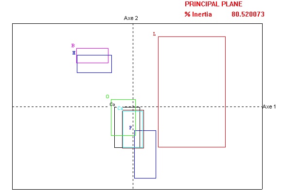
Figure 3: Principal plane of oils and fats data with Multidimensional Scaling.

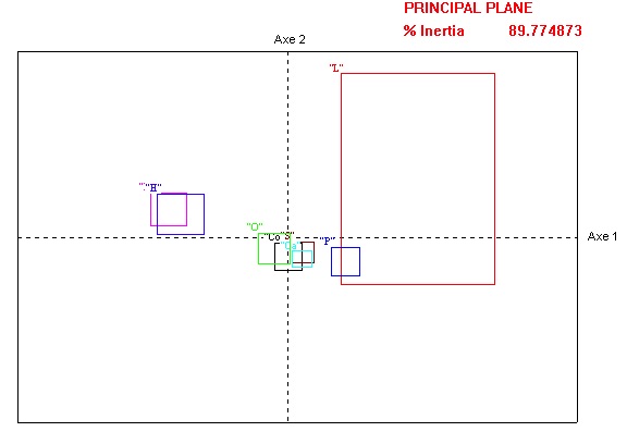
Figure 4: Principal plane of oils and fats data using Principal Component Analysis.

The clustering structure get in Figure 3 and in Figure 4 are similar because the groups are the same and the size of the rectangles are proportional. So the interpretation of both graphs will be just about the same.

The second data set we considered consists of dissimilarity judgments of rectangles of different area and height–to–width ratio, judged by 16 subjects. These data were presented in a paper on constrained multidimensional scaling, (Winsberg and De Soete (1997)). Other researchers have looked at rectangles. However, in general, they restricted their attention to rectangles where the height is greater than the width or vice versa. This data set includes both rectangles in which the height is greater than the width and vice versa. In a study of rectangle dominance data discussed by (Carroll (1972)) the consensus dimension corresponded fairly well with size; but it was also clear in that case that subjects vary greatly as to what they mean by size. Some subjects equated size to height, some to area, some to width, and some to height–to–width ratio. When Winsberg and De Soete (1997) analyzed their data for the 16 subjects, taken together, three dimensions were recovered: the first was area, which relates to size; the second dimension was height–to–width ratio, with recovered values falling into essentially three categories, depending on whether the height–to–width ratio was greater than, equal to, or less than one, which relates to the position of the rectangle, (up–down); the third was height–to–width ratio, or alternatively width–to–height ratio, such that the value was less than or equal to one, i.e. squareness. So, the first dimension relates to size, and the other two dimensions relate to shape. Three latent classes were found in the CLASCAL analysis. The difference among the classes was primarily due to how strongly they weighted dimension two.

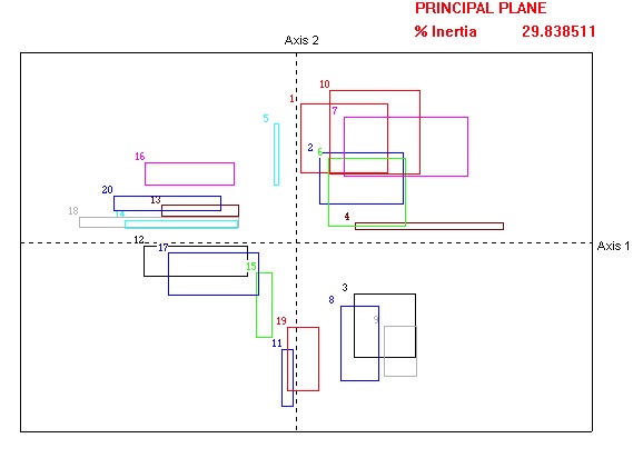
Figure 5: Rectangles whose height is less than their width on the right.

Our INTERSCAL solution for the data recovers the same three dimensions. Figures 5 and 6 display the results. The second dimension separates the rectangles whose height is less than their width at the up of Figure 5 form those whose height is greater than their width at the bottom of Figure 5. Dimension one is related to squareness, that is width–to–height ratio or height–to–width ratio whichever is less than one. The rectangles which are nearly square are on the right side of Figure 5. The third dimension is related to size or area with the smaller rectangles appearing on the top of Figure 6.

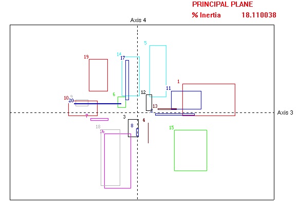
Figure 6: Third dimension related to size or area with the smaller rectangles appearing on the top.

Note that each stimulis/object is represented as a hypercube of three dimensions. Thus for rectangle number eight we have $a(w)=[Y_{1}(w)\in[4.43,7.22]]\wedge[Y_{2}(w)\in[-35.12,-14.94]]\wedge[Y_{3}(w)\in[-0.05,0.49]]$. The “psychological” rectangles occupy a hypercube so that for the physical stimulis/object rectangle number eight, the model of the corresponding psychological object is the symbolic object with a conjunction of three attributes, each described by an interval, one interval for up–down $[4.43,7.22]$, one interval for squareness or shape $[-35.12,-14.94]$, (height–to–width ratio or width–to–height ratio whichever is less than one), and one interval for area or size $[-0.05,0.49]$. Note that up–down is not precisely localized. It is represented by an interval for each symbolic object, even though the “physical” rectangles fall into three categories on this variable that is, up, (the height is greater than the width), down, (the width is greater than the height), or neither, (the rectangle is a square). Up–down is not precisely localized for each “psychological” rectangle, because for some of the judges, this dimension was more important than for others when making the dissimilarity judgements, causing the distance between the up rectangles and the down rectangles to be an interval. Note that the size of this interval is smaller for those rectangles which are more nearly square, that is those rectangles at the bottom of Figure 5.

These results are consistent with the results of the analyses presented in Winsberg and De Soete (1997). In addition, this new technique indicates how precisely the rectangles are located in the space. We have obtained the interesting result that the size of the hypercube occupied by a rectangle is inversely related to its area ($r=-0.72$). This finding indicates that it is easier for subjects to distinguish larger rectangles from one another than it is to do so for smaller rectangles.

4 Conclusion

We have presented a Multidimensional Scaling technique which enables the representation of objects as hypercubes in a $n$ dimensional space, reflecting a range of dissimilarities observed for each pair of objects. By representing these objects as hypercubes we can display information relating to how well the objects are localized. Moreover, as we demonstrated in the example dealing with rectangles the precision with which an object is localized may be related to one of its attributes.

This technique can be extended to include the case where in addition to the common dimensions shared by all the stimuli, some stimuli may possess specific attributes.

1. Bock, H-H and Diday, E. (eds.) (2000). Analysis of Symbolic Data. Exploratory methods for extracting statistical information from complex data. Springer Verlag, Heidelberg, 425 pages, ISBN 3-540-66619-2, 2000.

2. Borg I. and Groenen P. (1997). Modern Multidimensional Scaling – Theory and Applications, Springer–Verlag, New York.

3. Brito P. (1991). Analyse de donnees symboliques: Pyramides d’heritage, Thèse de doctorat, Université Paris 9 Dauphine.

4. Carroll, J.D. (1972). Individual Differences and Multidimensional Scaling. in Multidimensional Scaling Theory and Applications in the Behavioral Sciences, vol I, Theory, New York: Seminar Press.

5. Cazes P., Chouakria A., Diday E. et Schektman Y. (1997). Extension de l’analyse en composantes principales à des données de type intervalle, Rev. Statistique Appliquée, Vol. XLV Num. 3 pag. 5-24, France.

6. Cox T. and Cox M. (1994). Multidimensional Scaling, Chapman and Hall,New York.

7. Denoeux T. and Masson M. (1999). Multidimensional Scaling of interval–valued dissimilarity data. Université de Technologie de Compiégne, France.

8. Diday E., Lemaire J., Pouget J., Testu F. (1984). Eléments d’Analyse des données. Dunod, Paris.

9. Diday E. (1987). Introduction l’approche symbolique en Analyse des Donnés. Première Journées Symbolique-Numérique. Université Paris IX Dauphine.

10. Gower, J. C. (1966) Some distances properties of latent root and vector methods using multivariate analysis. Biometrika, 53, 325–338.

11. Torgenson, W. S. (1952) Multidimensional scaling: 1 Theory and method, Psychometrika, 17, 401–419.

12. Torgenson, W. S. (1958) Theory and methods of scaling. New York: Wiley.

13. Winsberg, S. and Desoete, G. (1997) Multidimensional scaling with constrained dimensions: CONSCAL, British Journal of Mathematical and Statistical Psychology, 50, 55-72.