D³GU: Multi-target Active Domain Adaptation
via Enhancing Domain Alignment

Abstract

Unsupervised domain adaptation (UDA) for image classification has made remarkable progress in transferring classification knowledge from a labeled source domain to an unlabeled target domain, thanks to effective domain alignment techniques. Recently, in order to further improve performance on a target domain, many Single-Target Active Domain Adaptation (ST-ADA) methods have been proposed to identify and annotate the salient and exemplar target samples. However, it requires one model to be trained and deployed for each target domain and the domain label associated with each test sample. This largely restricts its application in the ubiquitous scenarios with multiple target domains. Therefore, we propose a Multi-Target Active Domain Adaptation (MT-ADA) framework for image classification, named D³GU, to simultaneously align different domains and actively select samples from them for annotation. This is the first research effort in this field to our best knowledge. D³GU applies Decomposed Domain Discrimination (D³) during training to achieve both source-target and target-target domain alignments. Then during active sampling, a Gradient Utility (GU) score is designed to weight every unlabeled target image by its contribution towards classification and domain alignment tasks, and is further combined with KMeans clustering to form GU-KMeans for diverse image sampling. Extensive experiments on three benchmark datasets, Office31, OfficeHome, and DomainNet, have been conducted to validate consistently superior performance of D³GU for MT-ADA .

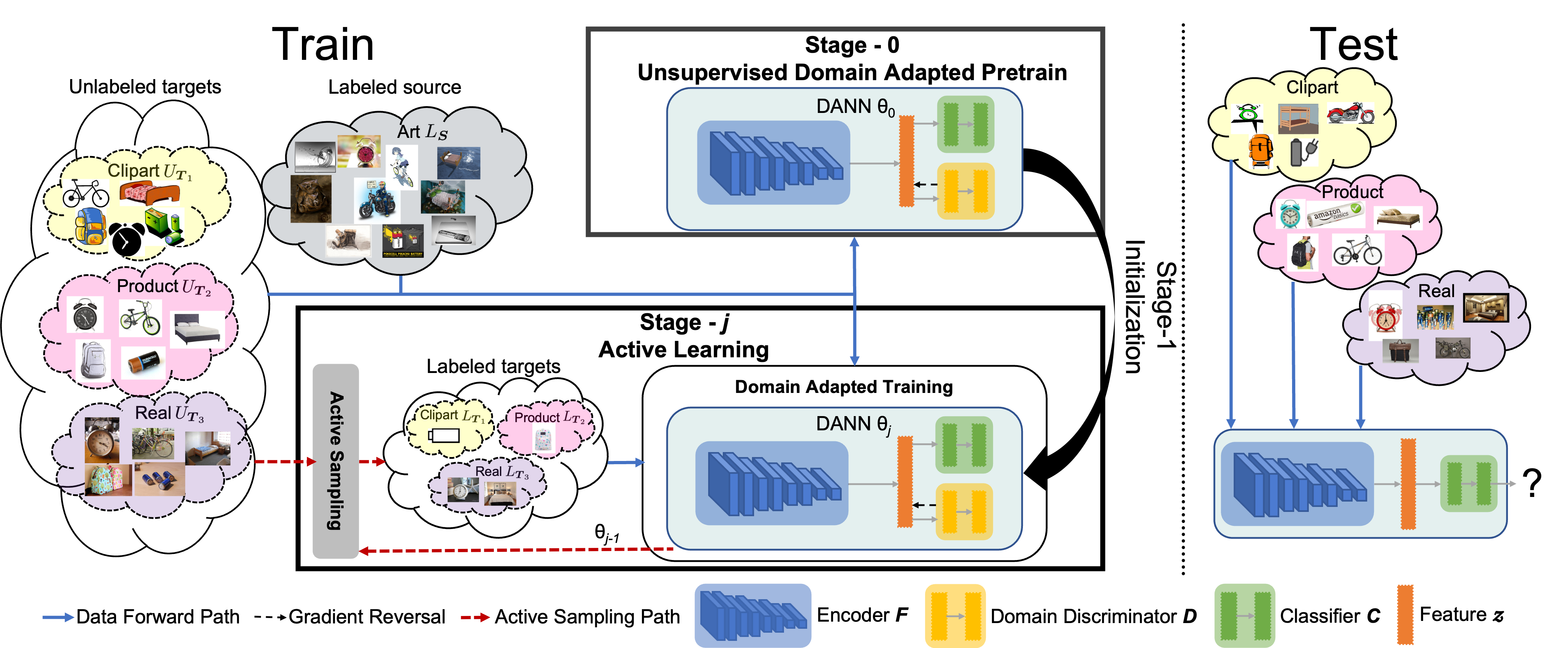
Figure 1: Illustration of MT-ADA task on OfficeHome with source domain (art), three target domains (clipart, product, real), and five classification classes (alarm_clock, backpack, batteries, bed, bike). The pretraining stage trains a model $\theta_{0}$ through unsupervised domain adaptation on labeled source images $L_{\mathcal{S}}$ and unlabeled target images $\bigcup\{U_{\mathcal{T}_{i}}\}_{i=1}^{3}$. Multiple active learning stages then follow to iterate between active sampling and domain adapted training. At the $j$-th active learning stage, the active sampling function selects and annotates some unlabeled target images to expand the labeled target set $\bigcup\{L_{\mathcal{T}_{i}}\}_{i=1}^{3}$ using the model $\theta_{j-1}$ trained at the previous stage. The domain adapted training step then finetunes $\theta_{j-1}$ to obtain $\theta_{j}$ using all images and annotations. Model performance is evaluated on target domains at test time. Section 3 describes more details.

1 Introduction

Deep image classification models trained in one domain (source) often fail to generalize well to other domains (targets) due to ubiquitous domain shifts. Domain shifts can occur due to a variety of reasons, such as changing conditions (e.g., background, location, pose changes) and different image formats (e.g., photos, NIR images, paintings, sketches) [9]. To address this problem, the challenging Unsupervised domain adaptation (UDA) paradigm has been extensively studied in recent years. Without any annotated data in the target domain $\mathcal{T}$, UDA aims to train a robust classification model for the target by transferring relevant knowledge from the labeled source domain $\mathcal{S}$. Various methods have emerged to approach the problem by aligning source and target feature distributions (Domain Alignment)  [27, 48, 5, 43, 25, 10, 1, 8, 49, 44, 16, 23, 19]. The most popular line of research designs adversarial domain discriminators in parallel with the classification head  [48, 20, 27]. Through adversarial training of the domain discriminator, the feature encoder learns a domain-invariant feature space with informative supervision from the source, while addressing the domain shifts between the source and the target. The success of domain adaptation thus heavily relies on effective alignment between domains.

Along with UDA, it has also been empirically established that a small number of labeled data in the target domain can largely improve the performance of domain adaptation [22]. Active Learning, the process of selecting labeled data, has then been identified as the critical factor for classification performance. This has motivated researchers to apply it to domain adaptation and formulate the problem of Single-Target Active Domain Adaptation (ST-ADA). ST-ADA aims to identify the most informative unlabeled target samples for manual annotation and efficiently mitigate the lack of classification knowledge in the target domain [20, 30, 34, 6, 7, 46, 14]. However, ST-ADA is not an ideal solution for many real-world scenarios where multiple target domains are available. Specifically, applying ST-ADA on multiple target domains requires independently training one model on each target domain. At test time, the domain label of a test sample should also be known to select its target model for inference. The whole system is therefore restricted by huge disk storage linearly increasing with number of target domains involved and its usage scenarios, necessitating a framework to be designed for Multi-Target Active Domain Adaptation (MT-ADA).

Therefore, we propose the first learning framework for MT-ADA image classification. As depicted in Figure 1, our framework consists of an initial pretraining stage, followed by multiple active learning stages. The pretraining stage conducts unsupervised domain adaptation with all labeled source images and unlabeled target images. Each active learning stage consists of two steps: (i) an active sampling step automatically selecting unlabeled target images from the union target pool for manual annotation within a preset budget. (ii) a domain adapted training step utilizing all images and available annotations to obtain an improved classification model. The iteration between these two steps gradually expands the labeled target set and improves classification performance on target domains. Unlike the aforementioned ST-ADA solution, our framework only maintains one classification model during both training and inference, and is domain-label-free at test time.

However, since every domain has its domain-specific classification information, domain alignment in MT-ADA becomes much more challenging. To address this problem, we focus on improving domain alignment efficacy for MT-ADA during both training and active sampling. To this end, we first propose decomposed domain discrimination (D³) for training, which is deployed in pretraining stage and every domain adapted training step. It decomposes multi-domain alignment into source-target and target-target domain alignment and balances them appropriately. Consequently, the well-aligned feature space can facilitate the encoding of domain-invariant features. Then during active sampling, we conceptualize domain adaptation as a multi-task learning process with two objectives: classification and domain alignment. We weight target images with their contributions to both tasks, which are computed as each target image’s feature gradients from classification and domain alignment losses, supervised by corresponding pseudo-labels. The computed weights, named Gradient Utility (GU), are further combined with KMeans clustering (GU-KMeans) to select diverse target samples for annotation. GU-KMeans thus is able to automatically distribute the preset budget among target domains and identify images that contribute maximally to domain adaptation. Our unified framework, named D³GU, effectively boosts MT-ADA performance via enhancing domain alignments during both training and active sampling.

In summary, our contribution is three-fold:

• To address the domain shifts during training in the multi-target setting, we introduce decomposed domain discrimination (D³) to appropriately achieve source-target and target-target domain alignments.

• We propose GU-KMeans, an active sampling strategy utilizing gradients from classification and domain alignment losses to select informative target images.

• To the best of our knowledge, this is the first work addressing the MT-ADA problem for image classification. Extensive experiments on Office31 [32], OfficeHome [41], and DomainNet [29] have demonstrated its state-of-the-art performance.

2 Related work

2.1 Unsupervised domain adaptation

To mitigate the domain shifts between source and target domains, modern unsupervised domain adaptation methods rely on various domain alignment techniques to align the distributions of source and target features. One line of research is to design various metrics to decrease the distance between source and target distributions [26, 25, 5, 43]. It is however difficult to comprehensively compute distribution disparity with handcrafted metrics. A more prominent line of work resorted to adversarial domain discriminators to automatically align domains via min-max optimization [48, 20, 27]. The pioneer work, DANN [48], included a binary domain discriminator in the network architecture and reversed its gradient flowing to the feature encoder during back-propagation. Recent UDA works were mostly built on the domain discriminator by proposing some improvement in architectures [1, 44, 45], training pipelines [16], and loss functions [8, 49, 23, 18, 40, 19]. Due to DANN’s popularity and the convention to use it on ADA [7, 20, 34, 30], our work is also built upon it to enhance domain alignment.

2.2 Multi-target domain adaptation

Real-world applications often require adaptation to multiple target domains. Research works for domain adaptation on multiple target domains can be classified into blended-target adaptation and multi-target adaptation, determined by the availability of target domain labels. When target domain labels are missing, blended-target domain adaptation methods [15, 50, 47] merge all targets into one and focus on source-target alignment. In this paper, we instead study multi-target domain adaptation (MTDA) [13, 28, 39, 31], where target domain labels are provided for training data. Previous MTDA methods proposed sophisticated training pipelines and architectures, including decomposed mapping [13], knowledge distillation [28, 39], and curriculum learning [31]. On the contrary, we propose a simple but effective adversarial domain discrimination technique to enhance multi-domain alignment, with minimal modifications to the training pipeline and architecture.

2.3 Active domain adaptation

Traditional active learning methods aim to selectively annotate images by measuring their importance as data uncertainty [33, 11, 37, 36] and diversity [35, 38, 12]. Recently, active domain adaptation (ADA), which instead actively annotates a few images from the target domain to address domain shifts, has received increasing research attention. AADA [20] weighted entropy score with target probability at the equilibrium state of adversarial training. TQS [7] jointly considered committee uncertainty, and domainness for active learning. CLUE [30] integrated entropy score into diversity sampling via KMeans clustering. SDM [46] boosted active domain adaptation accuracy with the help of a margin loss. LAMDA [34] selected domain-representative candidates. However, these methods treated classification and domain alignment as two independent tasks and failed to explicitly consider their correlations. In this paper, we leverage the domain discriminator to propose an active sampling criterion called gradient utility, which explicitly measures each target image’s contributions to classification and domain alignment.

3 Preliminary

3.1 Multi-target active domain adaptation

MT-ADA aims at training a single classification model for $K$ classes on $N$ target domains $\{\mathcal{T}_{i}\}_{i=1}^{N}$ by transferring classification knowledge from one labeled source domain $\mathcal{S}$. It utilizes labeled source images $L_{\mathcal{S}}$ and unlabeled target images $\{U_{\mathcal{T}_{i}}\}_{i=1}^{N}$, then selects and annotates images from $\{U_{\mathcal{T}_{i}}\}_{i=1}^{N}$ at multiple stages to build up labeled target set $\{L_{\mathcal{T}_{i}}\}_{i=1}^{N}$ to join training. As visualized in Figure 1, the learning process is composed of an initial unsupervised domain adapted pretraining stage (stage-$0$) followed by $s$ stages of active learning. The same domain adaptation method is used in all stages for training. The pretraining stage trains a model $\theta_{0}$ with only $L_{\mathcal{S}}$ and $\{U_{\mathcal{T}_{i}}\}_{i=1}^{N}$ in the UDA manner, since $\{L_{\mathcal{T}_{i}}\}_{i=1}^{N}=\emptyset$ initially. At the $j$-th active learning stage with annotation budget $b_{j}$, an active sampling algorithm first selects $b_{j}$ images from unlabeled target union $\{U_{\mathcal{T}_{i}}\}_{i=1}^{N}$ for annotation by utilizing the previous stage’s trained model $\theta_{j-1}$, and then moves the selected images from unlabeled target set to the labeled target set. Since the selection pool is the target union, numbers of images selected from each target domain, which have a sum of $b_{j}$, are automatically determined by the active sampling algorithm. Through domain adapted training, an improved model $\theta_{j}$ is thus obtained by finetuning $\theta_{j-1}$ on labeled source set $L_{\mathcal{S}}$, unlabeled target set $\{U_{\mathcal{T}_{i}}\}_{i=1}^{N}$, and labeled target set $\{L_{\mathcal{T}_{i}}\}_{i=1}^{N}$. The active learning stages repeat until the annotation budget runs out. At test time, we measure model’s average classification accuracy on all target domains.

3.2 Adversarial domain adaptation

Following previous convention [7, 20, 34, 30], we choose DANN [48] for domain adaptation due to its high efficiency. DANN is the exemplar of adversarial domain adaptation [48, 10, 27]. Initially designed for single-target domain adaptation, DANN has been adapted to multi-target domain adaptation by merging all target domains into a union domain $\tilde{\mathcal{T}}=\bigcup\{\mathcal{T}_{i}\}_{i=1}^{N}$ [39, 28, 42]. Specifically, as Figure 1 shows, the model is composed of three parts: a backbone feature encoder $F$, a classification head $C$, and a domain discrimination head $D$. During training, an input image $\boldsymbol{x}\in\mathcal{R}^{3\times H\times W}$ with height $H$ and width $W$ from either source domain $\mathcal{S}$ or target domain $\mathcal{\tilde{T}}$ is first encoded into a feature vector, i.e., $\boldsymbol{z}=F(\boldsymbol{x})$, which is then passed to $C$ and $D$ simultaneously. The classification head and a softmax layer predict $\boldsymbol{z}$ into class probabilities $\boldsymbol{p}=\text{Softmax}(C(\boldsymbol{z}))\in\mathcal{R}^{K}$. When $\boldsymbol{x}$ is labeled with class $y$, the classification loss is computed as:

$$\mathcal{L}_{cls}(\boldsymbol{x},y) =-\sum\nolimits_{k=1}^{K}\mathbbm{1}_{[k=y]}\,\text{log}\,\boldsymbol{p}_{k}$$ (1)

Parallelly, the domain discrimination branch predicts $\boldsymbol{z}$ into domain logits $\boldsymbol{\phi}^{d}=D(\boldsymbol{z})\in\mathcal{R}^{2}$, which is then activated into domain probabilities $\boldsymbol{q}\in\mathcal{R}^{2}$ by softmax layer. The two channels of $\boldsymbol{\phi}^{d}$ and $\boldsymbol{q}$ represent source and target domains, respectively. Suppose the domain label of $\boldsymbol{x}$ is $m$, a binary domain classification task is formulated with loss:

$$\mathcal{L}_{dom}^{bin}(\boldsymbol{x},m) =-\sum\nolimits_{t\in\{\mathcal{S},\mathcal{T}\}}\mathbbm{1}_{[t=m]}\,\text{log}\,\boldsymbol{q}_{t}$$ (2)

We denote it as binary domain discrimination. To achieve domain alignment, a domain-invariant feature encoder is needed to confuse the domain discriminator. Therefore, we adversarially train $D$ to minimize $\mathcal{L}_{dom}^{bin}$ and $F$ to maximize $\mathcal{L}_{dom}^{bin}$, which is implemented by reversing the gradients flowing from $D$ to $\boldsymbol{z}$. In practice, during all training steps, $\mathcal{L}_{dom}^{bin}$ is computed on all images because domain labels are always provided, while $\mathcal{L}_{cls}$ is only computed on labeled images. At test time, only the backbone $F$ and classification head $C$ are kept for inference.

4 Proposed method

4.1 Decomposed domain discrimination

Although binary domain discrimination already demonstrates appealing performance, the missing target domain labels make it focus on source-target alignment but ignore target-target alignment. As shown in Figure 2, this results in under-alignment between target domains, the distributions of which can be quite distinct and cause drastic category mismatch [50]. To ensure better alignment between multiple domains, all-way domain discrimination [31] is used to align every domain with all others. By predicting a logit for every domain, it estimates the probabilities of the input belonging to every domain out of all $(1+N)$ domains, i.e., $\boldsymbol{q}\in\mathcal{R}^{(1+N)}$. The corresponding loss function is then changed from Equation 2 to:

$$\mathcal{L}_{dom}^{aw}(\boldsymbol{x},m) =-\sum\nolimits_{t\in\{\mathcal{S},\mathcal{T}_{1},...,\mathcal{T}_{N}\}}\mathbbm{1}_{[t=m]}\,\text{log}\,\boldsymbol{q}_{t}$$ (3)

Similarly, we apply minmax optimization on $\mathcal{L}_{dom}^{aw}$ for adversarial training. In this way, every domain is aligned with the others, resulting in a more compact feature space.

However, while domain adaptation assumes most of the classification knowledge is shared and transferable between domains (“+”), every domain also has its own domain-specific classification knowledge (“-”), the alignment of which adversely affects the classification in the shared feature space. This is known as negative transfer [24, 51]. All-way domain discrimination applies the same degree of alignment between all domains, thus emphasizing alignment between unlabeled target domains where classification supervision is missing. Consequently, it can easily lead to negative transfer and over-alignment, as in Figure 2.

To mitigate this dilemma, we hereby propose Decomposed Domain Discrimination (D³) to decompose domain alignment into source-target alignment and target-target alignment. D³ uses a domain discriminator $D$ that predicts $(N+2)$-dimensional domain logits $\boldsymbol{\phi}^{d}\in\mathcal{R}^{(2+N)}$, corresponding to the source domain $\mathcal{S}$, union target domain $\tilde{\mathcal{T}}$, and each individual target domains $\mathcal{T}_{1},...,\mathcal{T}_{N}$, sequentially. It then simultaneously computes $\mathcal{L}_{dom}^{bin}$ on $\mathcal{S}$ and $\tilde{\mathcal{T}}$ for source-target alignment, and $\mathcal{L}_{dom}^{aw}$ on $\mathcal{S}$ and $\{\mathcal{T}_{i}\}_{i=1}^{N}$ for target-target alignment. Decomposed domain discrimination is thus formulated as a weighted sum of the two losses:

$$\mathcal{L}_{dom}^{dec}=\mathcal{L}_{dom}^{bin}+\alpha\mathcal{L}_{dom}^{aw}$$ (4)

where loss weight for $\mathcal{L}_{dom}^{bin}$ is always $1.0$ to necessitate and prioritize source-target alignment since annotations mostly come from the source domain. $\alpha$ is the hyperparameter that controls the balance between the source-target alignment and target-target alignment to avoid either under-alignment or over-alignment. We show in experiments that, despite its simplicity, decomposed domain discrimination effectively facilitates encoding domain-invariant features and improves domain adaptation performance.

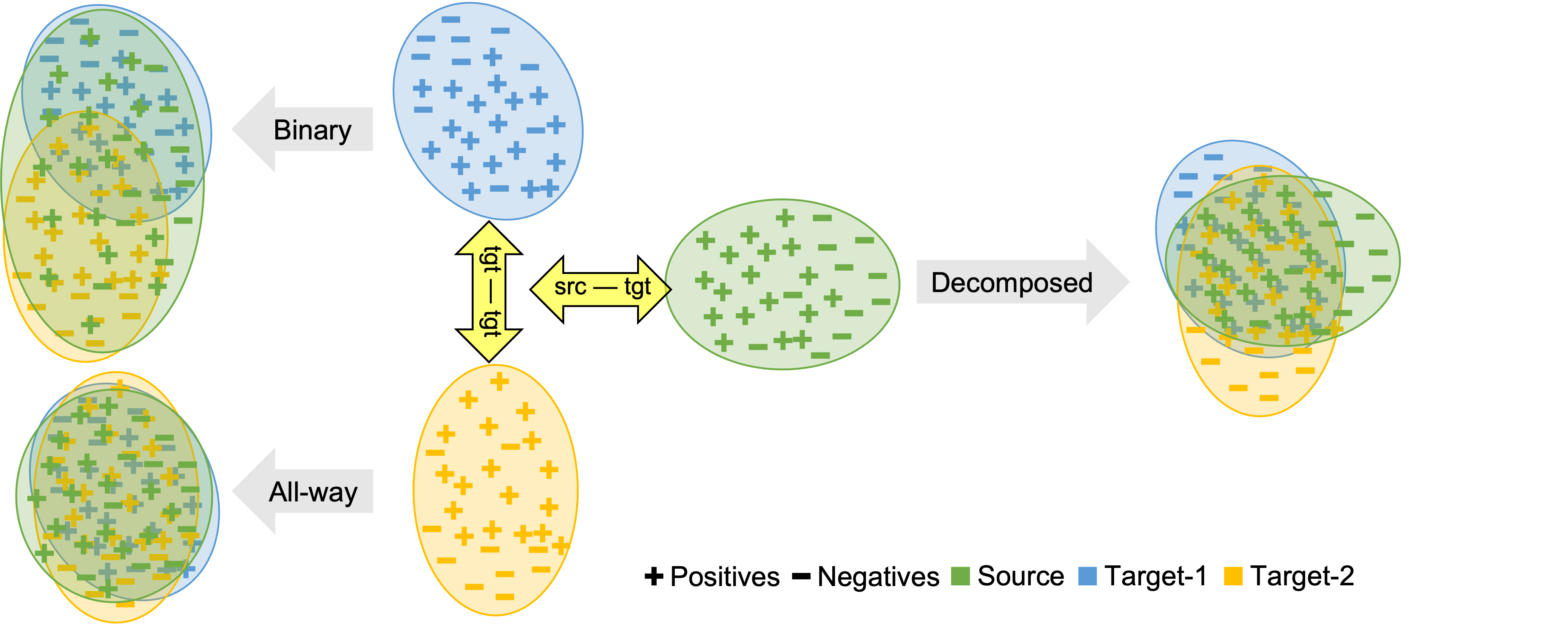
Figure 2: Each domain has its transferable positive knowledge (“+”), and negative knowledge (“-”) that is domain-specific and cannot be shared. Binary domain discrimination can lead to under-alignment between positives in the target domains while all-way domain discrimination leads to over-alignment of the negatives. Decomposed domain discrimination instead balances the two to enhance domain alignment.

4.2 Gradient utility for sample selection

Traditional active sampling functions consider unlabeled samples’ uncertainty as the major criterion for selection, i.e., samples closer to the decision boundaries are preferred. However, domain adaptation is a two-task learning process, where the classification task aims at learning classification knowledge from source domain and domain alignment task is responsible for knowledge transferring to the target domains. Merely applying the uncertainty-based methods to active domain adaptation, without addressing domain mismatch, can result in querying a sub-optimal set of samples. Existing active domain adaptation research therefore considers domain gap [20] and domain representatives [34]. However, they treat classification and domain alignment as two independent tasks and fail to consider their correlation.

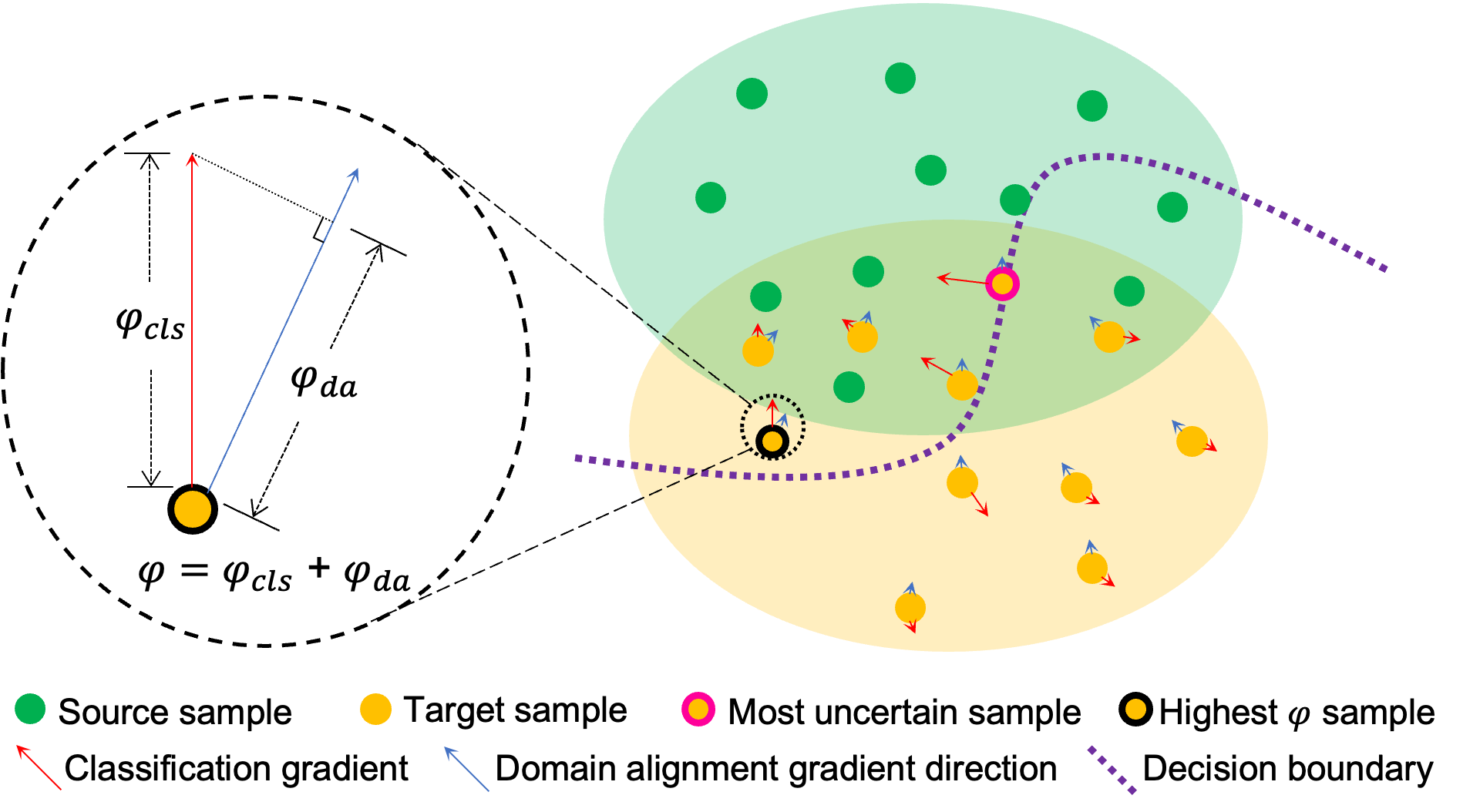
Figure 3: Gradient utility $\varphi$ measures each target sample’s contributions towards classification ($\varphi_{cls}$) and domain alignment ($\varphi_{da}$). Target samples with the highest $\varphi$, rather than the most uncertain ones, are upweighted the most.

We propose a novel technique to address this challenge by leveraging the domain discriminator. As mentioned in Section 3.2, the encoded feature $\boldsymbol{z}$ acts like a bridge between two task-specific branches $C$ and $D$. Our method thus quantifies the contributions of each sample in the encoded feature space, resulting from the active annotation, by measuring its gradient utilities towards these two branches.

Assuming the ideal situation where the classification label $y$ of a sample $\boldsymbol{x}$ is known, we firstly compute the negative gradient of the classification loss $\mathcal{L}_{cls}$ (supervised by the label $y$) w.r.t. its encoded feature $\boldsymbol{z}$:

$$\tilde{\boldsymbol{g}}_{cls}(\boldsymbol{x},y) =-\frac{\partial\mathcal{L}_{cls}(\boldsymbol{x},y)}{\partial\boldsymbol{z}}$$ (5)

which represents the first-order displacement of $\boldsymbol{z}$ in the feature space with both direction and magnitude, resulting from annotating it. Larger displacement induces larger changes to the feature space, leading to more contributions to the classification task. We can quantify such contribution with gradient utility towards classification, which is the magnitude of the displacement:

$$\varphi_{cls}(\boldsymbol{x},y) =\|\tilde{\boldsymbol{g}}_{cls}(\boldsymbol{x},y)\|_{2}$$ (6)

However, $\boldsymbol{x}$’s contribution to domain alignment task cannot be computed similarly, since the domain label $m$ is already known and active annotation does not augment any extra supervision. We therefore need another method to quantify the contribution resulting from annotating it with label $y$. To this end, we exploit the correlation between the classification and domain alignment tasks. Any attempt to optimize the performance of one task is likely to alter the encoded feature representations $\boldsymbol{z}$, which will affect the performance of the other task. Such task correlation can be computed by the cosine similarity between the two task gradients w.r.t. the encoded feature $\boldsymbol{z}$. Formally,

$$\tilde{\boldsymbol{g}}_{da}(\boldsymbol{x},\mathcal{S}) =-\frac{\partial\mathcal{L}_{dom}(\boldsymbol{x},\mathcal{S})}{\partial\boldsymbol{z}}$$ (7)

$$\text{corr}_{cls-da}(\boldsymbol{x},y,\mathcal{S}) =\frac{\tilde{\boldsymbol{g}}_{cls}(\boldsymbol{x},y)\boldsymbol{\cdot}\tilde{\boldsymbol{g}}_{da}(\boldsymbol{x},\mathcal{S})}{\|\tilde{\boldsymbol{g}}_{cls}(\boldsymbol{x},y)\|_{2}\cdot\|\tilde{\boldsymbol{g}}_{da}(\boldsymbol{x},\mathcal{S})\|_{2}}$$ (8)

where $\mathcal{L}_{dom}\in\{\mathcal{L}_{dom}^{bin},\mathcal{L}_{dom}^{aw},\mathcal{L}_{dom}^{dec}\}$ depending on which domain discrimination method is used, and $\tilde{\boldsymbol{g}}_{da}(\boldsymbol{x},\mathcal{S})$ is the negative gradient of the domain discrimination loss $\mathcal{L}_{dom}$ to align $\boldsymbol{x}$ with the source domain. Now we can derive target $\boldsymbol{x}$’s gradient utility towards domain alignment, resulting from annotating $x$ with label $y$:

$$\varphi_{da}(\boldsymbol{x},y) =\varphi_{cls}(\boldsymbol{x},y)\cdot\text{corr}_{cls-da}(\boldsymbol{x},y,\mathcal{S})$$ (9)

which measures how $\boldsymbol{x}$’s displacement in the feature space induced by classification affects domain alignment. We sum the gradient utilities towards both classification and domain alignment to form the final Gradient Utility (GU):

$$\varphi(\boldsymbol{x},y) =\varphi_{cls}(\boldsymbol{x},y)+\varphi_{da}(\boldsymbol{x},y)$$ (10)

which measures $\boldsymbol{x}$’s contribution to both tasks. We weight samples using their GUs during active sampling, as illustrated in Figure 3. In practice, the assumption on the availability of the ground truth label $y$ does not hold when sampling. We therefore use the predicted pseudo-label instead, which also shows strong empirical performance.

4.3 GU-KMeans for diverse sample selection

To further augment the selected target subset with diversity, at the $j$-th active sampling step, we cluster the unlabeled target images into $b_{j}$ clusters, where $b_{j}$ is the annotation budget mentioned in Section 3.1. The image closest to the centroid of each cluster is selected for annotation. KMeans is employed for clustering in our experiments following [30, 3]. The proposed gradient utilities act as sample weights when computing the centroids:

$$w(\boldsymbol{x}) =\text{norm}(\varphi(\boldsymbol{x}))^{\beta}$$ (11)

where $w$ is the sample weight and the “norm” operator divides all scores by the maximum to normalize them into the range $[0,1]$ for computational stability. A parameter $\beta$ is used as the exponent on the score to tradeoff gradient utility and diversity in active sampling. The larger $\beta$ is, the more importance we put on gradient utility than diversity. The final active sampling method is named as GU-KMeans.

5 Experiments and results

In the absence of benchmarks for MT-ADA for image classification, we develop our own codebase on three conventional domain adaptation datasets. We present experimental setup in Section 5.1, introduce baselines in Section 5.2, analyze the performance of our framework in Section 5.3, and provide more analysis in Section 5.4. Additional details and results are in the supplementary material.

5.1 Experimental setup

Datasets: We conduct multi-target active domain adaptation experiments on 3 benchmark datasets: Office31 [32], OfficeHome [41], and DomainNet [29]. Office31 consists of $4,652$ images classified into $31$ classes from $3$ domains {amazon, dslr, webcam}. OfficeHome consists of $15,500$ images spanning $65$ classes and $4$ domains {art, clipart, product, real}. DomainNet is a large-scale dataset with $0.6$ million images spanning $345$ classes and $6$ domains {clipart, infograph, painting, quickdrarw, real, sketch}. Since Office31 and OfficeHome do not provide train and test splits, we follow the conventional protocol to use all images for both training and testing [46, 30, 34, 7]. We use the official train/test splits in DomainNet for experiments.

Evaluation metric: For each dataset, when taking one domain as the source, we use all the remaining domains as targets, and report the averaged classification accuracy over all target domains. For example, on OfficeHome, reported accuracy corresponding to “art” refers to the average classification accuracy on clipart, product, and real, when taking art as the source. All reported results are the average of three random trials, unless otherwise specified.

Implementation: We use a ResNet-50 [21] pretrained on ImageNet [17, 2] as the backbone. Encoded feature dimension is $256$ on Office31/OfficeHome and $512$ on DomainNet. The classification head is a single layer neural network and the domain discriminator is a three-layer neural network with dropout value of $0.5$. $\alpha$ in Equation 4 is set to $1.0$ on Office31/OfficeHome and $0.05$ on DomainNet. $\beta$ in Equation 11 is set to $4.0$. We use SGD optimizer in unsupervised pretraining with learning rate $0.001$ and domain adapted training with learning rate $0.0003$, both of which are inversely decayed during training. We conduct $4$ active learning stages with equal annotation budget at each stage.

Method	Office31								OfficeHome
	budget=30/stage-1				budget=120/stage-4				budget=100/stage-1					budget=400/stage-4
	amzn	dslr	web	AVG	amzn	dslr	web	AVG	art	clip	prod	real	AVG	art	clip	prod	real	AVG
random(b)	85.38	81.14	81.44	82.65	92.64	85.03	85.75	87.80	63.37	62.43	56.78	63.64	61.55	68.20	68.47	61.99	68.15	66.70
entropy(b)	89.62	81.11	81.53	84.08	98.16	86.44	87.20	90.60	63.27	63.80	57.17	63.44	61.92	70.05	71.35	65.25	70.19	69.21
margin(b)	89.80	82.24	83.46	85.16	98.92	87.89	87.75	91.52	63.75	64.98	57.90	64.31	62.73	71.12	71.86	65.79	70.64	69.85
coreset(b)	85.52	80.50	81.08	82.36	90.51	83.22	83.41	85.71	62.00	62.75	55.23	62.94	60.73	66.48	67.22	60.38	66.47	65.14
BADGE(b)	89.16	81.61	82.86	84.54	98.54	86.53	87.82	90.97	64.25	64.65	57.38	64.57	62.71	70.70	72.14	64.57	70.28	69.42
AADA(a)	89.32	80.70	82.76	84.26	98.34	86.01	87.10	90.48	63.72	64.56	57.85	64.89	62.76	70.28	71.65	64.87	70.32	69.28
SDM(a)	89.85	81.94	83.55	85.11	99.06	87.62	88.32	91.67	64.23	64.85	58.09	65.65	63.21	71.03	72.72	65.88	70.92	70.13
LAMDA(a)	90.74	82.34	83.49	85.52	98.57	87.60	88.30	91.49	65.44	64.37	58.55	65.74	63.52	70.87	71.61	65.46	70.58	69.63
CLUE(a)	90.74	84.21	84.12	86.36	97.93	87.74	88.86	91.51	66.02	65.36	59.40	65.79	64.14	71.75	71.33	64.89	70.56	69.63
D3GU	91.14	84.23	85.16	86.84	99.16	88.55	89.29	92.33	65.96	66.53	59.29	66.30	64.52	72.36	72.65	65.75	71.43	70.55

Table 1: MT-ADA accuracies with total budget 120 and 400 on Office31 and OfficeHome, respectively. We conducted 4 active learning stages with equal budgets. Pretraining stage and active learning training stages apply the same domain discrimination, which is indicated by “(a)”(all-way) and “(b)”(binary) postfixes in “Method” column. We mark the best results in bold and underline the second-best ones. The best average results across all the source domains on each dataset are marked in red. Same annotations are used for Table 2 and 3.

5.2 Active sampling baselines

For replication purposes and fair comparison, we re-implemented the following active sampling baselines on our codebase, including both classical active sampling methods denoted as AL, and state-of-the-art active domain adaptation sampling methods denoted as ADA.

Entropy(AL) selects samples with the largest entropy scores, i.e., $\mathcal{H}(\boldsymbol{x})=-\sum_{k=1}^{C}\boldsymbol{p}_{k}(\boldsymbol{x})\ \text{log}\ \boldsymbol{p}_{k}(\boldsymbol{x})$, where $C$ and $\boldsymbol{p}$ refer to the number of classes and predicted class probabilities, respectively.

Margin(AL) selects samples with the smallest prediction margins $\mathcal{M}(\boldsymbol{x})=\boldsymbol{p}_{c_{1}}(\boldsymbol{x})-\boldsymbol{p}_{c_{2}}(\boldsymbol{x})$, where $c_{1}/c_{2}$ stands for the most/second-most confident predicted classes.

Coreset [35](AL) selects representative target subset with greedy KCenter clustering.

BADGE [4](AL) uses KMeans++ clustering on the classification gradient embedding space to select the most uncertain and diverse subset.

AADA [20](ADA) selects images with the largest augmented entropy scores, i.e., $G(\boldsymbol{x})=\frac{1-\boldsymbol{q}_{\mathcal{S}}(\boldsymbol{x})}{\boldsymbol{q}_{\mathcal{S}}(\boldsymbol{x})}\mathcal{H}(\boldsymbol{x})$, where $\boldsymbol{q}$/$\mathcal{S}$ refers to predicted domain probabilities/source domain.

CLUE [30](ADA) performs KMeans clustering on all target images with entropy scores as clustering weights. It however ignores domain shifts.

LAMDA [34](ADA) selects a subset of target images whose maximal mean discrepancy with the unlabeled target set is minimized. Selected images are representatives of the target domain but do not optimize classification accuracy.

SDM [46](ADA) improves margin sampling by further selecting images with strong correlations between the loss and the margin sampling function.

5.3 Main results

Method	C	I	P	Q	R	S	AVG
SDM(b)	43.06	43.26	43.82	40.42	42.97	46.41	43.32
CLUE(b)	43.79	46.48	44.41	40.03	43.01	46.71	44.07
LAMDA(b)	44.08	46.34	44.75	40.73	43.25	46.94	44.35
D3GU	44.40	47.23	44.82	40.90	43.23	47.13	44.62

Table 2: MT-ADA accuracies on DomainNet with total budget ${=}10,000$ in $4$ active learning stages. Capital letters are short for source domains. Refer to supplementary material for more results.

We compare our unified framework D³GU with baselines on MT-ADA task on Office31/OfficeHome in Table 1 and DomainNet in Table 2. In Table 3, we compare different domain adaptation methods at the pretraining stage (stage-$0$). We mainly compare with ADA baselines since they generally perform better than AL methods on ADA tasks. Results of ADA baselines are trained with domain adaptation methods whose empirical performances are better, i.e., all-way domain discrimination on Office31 and OfficeHome, and binary domain discrimination on DomainNet, as indicated in Table 3. We include more results in the supplementary material, including comparison between GU-KMeans and other sampling algorithms under the same domain adaptations on both MT-ADA and ST-ADA tasks.

DA	Office31			OfficeHome				DomainNet
	amzn	dslr	web	art	clip	prod	real	C	I	P	Q	R	S
binary	79.83	79.83	80.37	60.65	58.33	52.92	61.70	31.28	28.28	30.62	11.07	30.99	35.75
all-way	81.12	80.43	80.62	61.50	58.80	54.57	62.70	30.28	27.90	30.59	10.59	30.25	34.11
D3	81.13	80.16	80.66	61.79	59.26	54.77	63.07	31.43	28.46	30.69	11.43	30.75	35.59

Table 3: Unsupervised domain adaptation results of $3$ domain adaptations (DA) on Office31, OfficeHome, and DomainNet.

Performance of D³GU: As shown in Tables 1 and 2, D³GU consistently outperforms all baselines on almost every MT-ADA setting on three benchmark datasets. Under the settings where it does not achieve the best results, its accuracies still stay very close to the best ones. In Table 1, while SDM demonstrates competitive performance at stage-$4$ (AVG=$91.67/70.13$ on Office31/OfficeHome), it performs relatively poor at stage-$1$ (AVG=$85.11/63.21$ on Office31/OfficeHome). In comparison, D³GU demonstrates consistent state-of-the-art performance at both stages. This unanimously corroborates the promise of D³GU for real-world multi-target active domain adaptation applications.

Performance of decomposed domain discrimination: As shown in Table 3, neither binary domain discrimination nor all-way discrimination shows consistent advantages on all three datasets. On DomainNet, where the $6$ domains and large number of images make domain shift a much more challenging problem to solve, all-way domain discrimination loses its advantage and falls behind binary discrimination by a large margin. This further suggests the existence of negative transfer. On the contrary, D³ always demonstrates the best or second-best accuracies, highlighting its superior and robust performance.

Performance of GU-KMeans: As shown in Figure 4, with the same domain discrimination methods, GU-KMeans still outperforms the other ADA baselines on all three datasets by a large margin. We also provide more experiment results in the supplementary material, which further shows GU-KMeans’s state-of-the-art performance as an active sampling method on Office31, OfficeHome, and DomainNet.

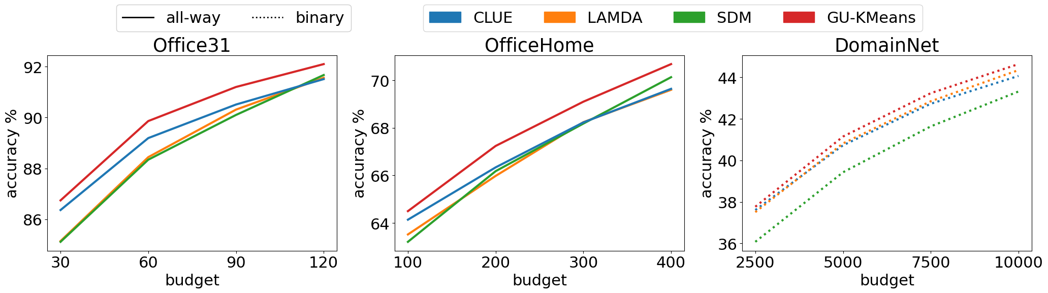
Figure 4: Plot of MT-ADA accuracies at $4$ active learning stages. We plot classification accuracies averaged over all source domains on each dataset (AVG in Tables 1, 2).

5.4 Further analysis

Analysis of each component of GU-KMeans: In Table 4, we validate the effectiveness of each component of GU-KMeans with real as source on OfficeHome. We first establish two baselines that select target images whose gradient utility scores ($\varphi_{cls}$ and $\varphi_{cls}+\varphi_{da}$) are highest, similar to entropy sampling. While entropy score sampling improves random sampling by a large margin with budget = $400$, gradient utility towards classification $\varphi_{cls}$ proves to be a more effective way to measure samples’ contribution to classification (Cls), further improving entropy sampling significantly in both budget settings. By further considering samples’ contribution to domain alignment (Da) by introducing $\varphi_{da}$, performance keeps increasing to $70.84$ with budget = $400$, already outperforming the second best accuracy $70.64$ of margin sampling as indicated in Table 1. GU-KMeans further boosts the performance by introducing KMeans for diversity (Div). These results show the usefulness of each component of GU-KMeans as an active sampling method.

Ablation on decomposed loss weight parameter: We plot the unsupervised domain adaptation pretraining results with various $\alpha$ values (Equation 4) in the top subfigure of Figure 5, with source domain quickdraw on DomainNet. quickdraw is the most challenging source domain in DomainNet, where the objects are only outlined by several black lines. With binary discrimination as the baseline, $\alpha$ around $0.2$ gives the best tradeoff between source-target alignment and target-target alignment. The larger value of $\alpha$ leads to over-alignment and makes performance worse, with the worst performance achieved with only all-way discrimination. We report distances between domains of different $\alpha$ values to quantify domain alignment in the supplementary material.

Ablation on utility-diversity tradeoff parameter: As shown in the bottom subfigure of Figure 5, we ablate the utility-diversity tradeoff parameter $\beta$ (Equation 11), taking art as source domain on OfficeHome. By introducing vanilla gradient utility as weight, performance of KMeans sampling is boosted by a large margin ($\beta=1.0$). While the best accuracy is obtained when $\beta\approx 4.0$, any value of $\beta$ in the range $[2.0,6.0]$ gives competitive performance.

Analysis of the number of samples selected from each target domain: In Figure 6, taking art as source domain on OfficeHome, we plot the accuracies and the numbers of selected samples in each target domain at every active learning stage, with annotation budget being $100$ at each stage. Note that active sampling always relies on the model trained at previous stage. As shown in the figure, D³GU tends to select more samples from the domain with worse performance. We also include selected samples’ distribution visualizations in the supplementary material.

Method	Cls	Da	Div	b=100	b=400
random	✗	✗	✗	63.64	68.15
entropy	✓	✗	✗	63.44-0.20	70.19+2.04
$\varphi_{cls}$	✓	✗	✗	64.48+1.04	70.61+0.42
$\varphi_{cls}+\varphi_{da}$	✓	✓	✗	64.90+0.42	70.84+0.23
GU-KMeans	✓	✓	✓	65.00+0.10	71.11+0.27

Table 4: Analysis of GU-KMeans with real as source on OfficeHome.“b” is short for budget.

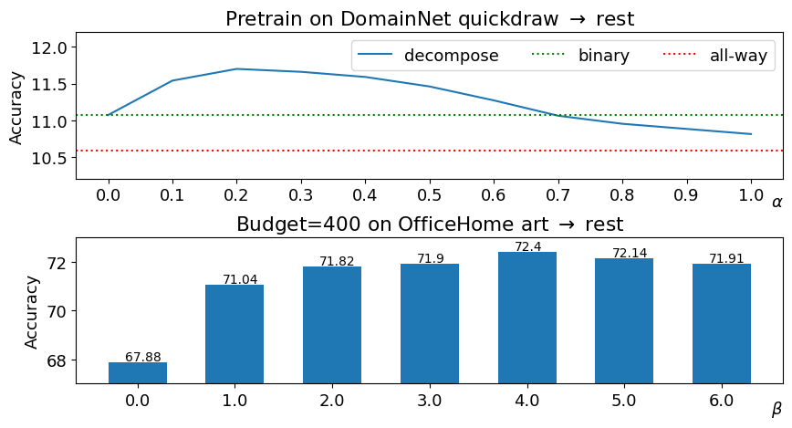
Figure 5: Top: UDA pretrain performances of different $\alpha$ values in Equation 4 with quickdraw as source domain on DomainNet. Bottom: Effect of $\beta$ values in Equation 11 on GU-KMeans $+$ binary domain discrimination, with art as source domain on OfficeHome.

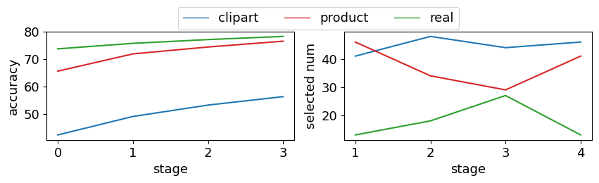
Figure 6: Accuracy and selected image counts for each target domain at every active learning stage using D³GU. Experiments conducted with art as source on OfficeHome.

6 Conclusion

In this paper, we propose D³GU, the first framework of its kind to address the challenging but unexplored task of multi-target active domain adaptation (MT-ADA) for image classification. We introduced decomposed domain discrimination to properly align source-target and target-target domains. We proposed an active sampling strategy that computes the gradient utilities of each target sample towards classification and domain alignment tasks, and combine it with KMeans for diversity. Extensive analysis on three datasets corroborates the promise of D³GU for MT-ADA. We hope our work will motivate the development of other MT-ADA algorithms for image recognition. When images and domains scale up, training may require extensive computing resources, impacting the environment negatively. We leave it as a future work to design more efficient algorithms.

7 Acknowledgement

This research was supported in part by the National Science Foundation under Grant Number: IIS-2143424 (NSF CAREER Award).

References

- [1] Kumar Abhishek, Sattigeri Prasanna, Wadhawan Kahini, Karlinsky Leonid, Feris Rogerio, T. Freeman William, and Wornell Gregory. Co-regularized alignment for unsupervised domain adaptation. In NeurIPS, 2018.
- [2] Paszke Adam, Gross Sam, Massa Francisco, Lerer Adam, Bradbury James, Chanan Gregory, Killeen Trevor, Lin Zeming, Gimelshein Natalia, Antiga Luca, Desmaison Alban, Köpf Andreas, Yang Edward, DeVito Zach, Raison Martin, Tejani Alykhan, Chilamkurthy Sasank, Steiner Benoit, Fang Lu, Bai Junjie, and Chintala Soumith. Pytorch: An imperative style, high-performance deep learning library. In NeuraIPS, 2019.
- [3] Parvaneh Amin, Abbasnejad Ehsan, Teney Damien, Haffari Reza, van den Hengel Anton, and Shi Javen Qinfeng. Active learning by feature mixing. In CVPR, 2022.
- [4] Jordan T Ash, Chicheng Zhang, Akshay Krishnamurthy, John Langford, and Alekh Agarwal. Deep batch active learning by diverse, uncertain gradient lower bounds. 2020.
- [5] Sun Baochen, Feng Jiashi, and Saenko Kate. Return of frustratingly easy domain adaptation. In AAAI, 2016.
- [6] Xie Binhui, Yuan Longhui, Li Shuang, Liu Chi Harold, Cheng Xinjing, and Wang Guoren. Active learning for domain adaptation: An energy-based approach. In AAAI, 2022.
- [7] Fu Bo, Cao Zhangjie, Wang Jianmin, and Long Mingsheng. Transferable query selection for active domain adaptation. In CVPR, 2021.
- [8] Chen Chao, Chen Zhihong, Jiang Boyuan, and Jin Xinyu. Joint domain alignment and discriminative feature learning for unsupervised deep domain adaptation. In AAAI, 2019.
- [9] Gabriela Csurka. Domain adaptation for visual applications: A comprehensive survey. In Domain Adaptation in Computer Vision Applications, 2017.
- [10] Tzeng Eric, Hoffman Judy, Saenko Kate, and Darrell Trevor. Adversarial discriminative domain adaptation. In CVPR, 2017.
- [11] Yarin Gal, Riashat Islam, and Zoubin Ghahramani. Deep bayesian active learning with image data. In International Conference on Machine Learning, pages 1183–1192. PMLR, 2017.
- [12] Yonatan Geifman and Ran El-Yaniv. Deep active learning over the long tail. 2017.
- [13] Behnam Gholami, Pritish Sahu, Ognjen Rudovic, Konstantinos Bousmalis, and Vladimir Pavlovic. Unsupervised multi-target domain adaptation: An information theoretic approach. 2020.
- [14] Rangwani Harsh, Jain Arihant, K Aithal Sumukh, and Babu R. Venkatesh. S3vaada: Submodular subset selection for virtual adversarial active domain adaptation. In ICCV, 2021.
- [15] Yu Huanhuan, Hu Menglei, and Chen Songcan. Multi-target unsupervised domain adaptation without exactly shared categories. In arXiv, 2018.
- [16] Na Jaemin, Jung Heechul, Jin Chang Hyung, and Hwang Wonjun. Fixbi: Bridging domain spaces for unsupervised domain adaptation. In CVPR, 2021.
- [17] Deng Jia, Dong Wei, Socher Richard, Li Li-Jia, Li Kai, and Li Fei-Fei. Imagenet: A large-scale hierarchical image database. In CVPR, 2009.
- [18] Hu Jian, Zhong Haowen, Yang Fei, Gong Shaogang, Wu Guile, and Yan Junchi. Learning unbiased transferability for domain adaptation by uncertainty modeling. In ECCV, 2022.
- [19] Huang Jiaxing, Guan Dayan, Lu Aoran, Xiao aand Shijian, and Shao Ling. Category contrast for unsupervised domain adaptation in visual tasks. In CVPR, 2022.
- [20] Su Jong-Chyi, Tsai Yi-Hsuan, Sohn Kihyuk, and Buyu Liu. Active adversarial domain adaptation. In CVPRW, 2019.
- [21] He Kaiming, Zhang Xiangyu, Ren Shaoqing, and Sun Jian. Deep residual learning for image recognition. In CVPR, 2016.
- [22] Saito Kuniaki, Kim Donghyun, Sclaroff Stan, Darrell Trevor, and Saenko Kate. Semi-supervised domain adaptation via minimax entropy. In ICCV, 2019.
- [23] Hu Lanqing, Kan Meina, Shan Shiguang, and Chen Xilin. Unsupervised domain adaptation with hierarchical gradient synchronization. In CVPR, 2020.
- [24] Rosenstein Michael T., Marx Zvika, Pack Kaelbling Leslie, and G. Dietterich Thomas. To transfer or not to transfer. In NeurIPS workshop on transfer learning, 2005.
- [25] Long Mingsheng, Zhu Han, Wang Jianmin, and I. Jordan Michael. Deep transfer learning with joint adaptation network. In ICML, 2017.
- [26] Long Mingsheng, Cao Yue, Wang Jianmin, and I. Jordan Michael. Learning transferable features with deep adaptation networks. In ICML, 2015.
- [27] Long Mingsheng, Cao Zhangjie, Wang Jianmin, and I. Jordan Michael. Conditional adversarial domain adaptation. In NeurIPS, 2018.
- [28] Le Thanh Nguyen-Meidine, Atif Belal, Madhu Kiran, Jose Dolz, Louis-Antoine Blais-Morin, and Eric Granger. Unsupervised multi-target domain adaptation through knowledge distillation. In WACV, 2021.
- [29] Xingchao Peng, Qinxun Bai, Xide Xia, Zijun Huang, Kate Saenko, and Bo Wang. Moment matching for multi-source domain adaptation. In ICCV, 2019.
- [30] Viraj Prabhu, Arjun Chandrasekaran, Kate Saenko, and Judy Hoffman. Active domain adaptation via clustering uncertainty-weighted embeddings. In ICCV, 2021.
- [31] Subhankar Roy, Evgeny Krivosheev, Zhun Zhong, Nicu Sebe, and Elisa Ricci. Curriculum graph co-teaching for multi-target domain adaptation. In Proceedings of the IEEE/CVF Conference on Computer Vision and Pattern Recognition, pages 5351–5360, 2021.
- [32] Kate Saenko, Brian Kulis, Mario Fritz, and Trevor Darrell. Adapting visual category models to new domains. In ECCV, 2010.
- [33] Greg Schohn and David Cohn. Less is more: Active learning with support vector machines. In ICML, volume 2, page 6. Citeseer, 2000.
- [34] Hwang Sehyun, Lee Sohyun, Kim Sungyeon, Ok Jungseul, and Kwak Suha. Combating label distribution shift for active domain adaptation. In ECCV, 2022.
- [35] Ozan Sener and Silvio Savarese. Active learning for convolutional neural networks: A core-set approach. In ICLR, 2018.
- [36] Inkyu Shin, Dong-Jin Kim, Jae Won Cho, Sanghyun Woo, Kwanyong Park, and In So Kweon. Labor: Labeling only if required for domain adaptive semantic segmentation. In Proceedings of the IEEE/CVF International Conference on Computer Vision, pages 8588–8598, 2021.
- [37] Yawar Siddiqui, Julien Valentin, and Matthias Nießner. Viewal: Active learning with viewpoint entropy for semantic segmentation. In Proceedings of the IEEE/CVF conference on computer vision and pattern recognition, pages 9433–9443, 2020.
- [38] Samarth Sinha, Sayna Ebrahimi, and Trevor Darrell. Variational adversarial active learning. In Proceedings of the IEEE/CVF International Conference on Computer Vision, pages 5972–5981, 2019.
- [39] Isobe Takashi, Jia Xu, Chen Shuaijun, He Jianzhong, Shi Yongjie, Liu Jianzhuang, Lu Huchuan, and Wang Shengjin. Multi-target domain adaptation with collaborative consistency learning. In CVPR, 2021.
- [40] Kalluri Tarun, Sharma Astuti, and Chandraker Manmohan. Memsac: Memory augmented sample consistency for large scale domain adaptation. In ECCV, 2022.
- [41] Hemanth Venkateswara, Jose Eusebio, Shayok Chakraborty, and Sethuraman Panchanathan. Deep hashing network for unsupervised domain adaptation. In CVPR, 2017.
- [42] Kumar Vikash, Lal Rohit, Patil Himanshu, and Chakraborty Anirban. Conmix for source-free single and multi-target domain adaptation. In WACV, 2023.
- [43] Zellinger Werner, Lughofer Edwin, Saminger-Platz Susanne, Grubinger Thomas, and Natschlager Thomas. Central moment discrepancy (cmd) for domain-invariant representation learning. In ICLR, 2017.
- [44] Chang Woong-Gi, You Tackgeun, Seo Seonguk, Kwak Suha, and Han Bohyung. Domain-specific batch normalization for unsupervised domain adaptation. In CVPR, 2019.
- [45] Gu Xiang, Sun Jian, and Xu Zongben. Spherical space domain adaptation with robust pseudo-label loss. In CVPR, 2020.
- [46] Ming Xie, Yuxi Li, Yabiao Wang, Zekun Luo, Zhenye Gan, Zhongyi Sun, Mingmin Chi, Chengjie Wang, and Pei Wang. Learning distinctive margin toward active domain adaptation. In CVPR, 2022.
- [47] Peng Xingchao, Huang Zijun, Sun Ximeng, and Saenko Kate. Domain agnostic learning with disentangled representations. In ICML, 2019.
- [48] Ganin Yaroslav and Lempitsky Victor. Unsupervised domain adaptation by backpropagation. In ICML, 2015.
- [49] Gao Zhiqiang, Zhang Shufei, Huang Kaizhu, Wang Qiufeng, and Zhong Chaoliang. Gradient distribution alignment certificates better adversarial domain adaptation. In ICCV, 2021.
- [50] Chen Ziliang, Zhuang Jingyu, Liang Xiaodan, and Lin Liang. Blending-target domain adaptation by adversarial meta-adaptation networks. In CVPR, 2019.
- [51] Wang Zirui, Dai Zihang, Poczos Barnabas, and Carbonell Jaime. Characterizing and avoiding negative transfer. In CVPR, 2019.