State-Specific Coupled-Cluster Methods for Excited States

Abstract

We reexamine $\Delta$CCSD, a state-specific coupled-cluster (CC) with single and double excitations (CCSD) approach that targets excited states through the utilization of non-Aufbau determinants. This methodology is particularly efficient when dealing with doubly excited states, a domain where the standard equation-of-motion CCSD (EOM-CCSD) formalism falls short. Our goal here is to evaluate the effectiveness of $\Delta$CCSD when applied to other types of excited states, comparing its consistency and accuracy with EOM-CCSD. To this end, we report a benchmark on excitation energies computed with the $\Delta$CCSD and EOM-CCSD methods, for a set of molecular excited-state energies that encompasses not only doubly excited states but also doublet-doublet transitions and (singlet and triplet) singly-excited states of closed-shell systems. In the latter case, we rely on a minimalist version of multireference CC known as the two-determinant CCSD method to compute the excited states. Our dataset, consisting of 276 excited states stemming from the quest database [Véril et al., WIREs Comput. Mol. Sci. 2021, 11, e1517], provides a significant base to draw general conclusions concerning the accuracy of $\Delta$CCSD. Except for the doubly-excited states, we found that $\Delta$CCSD underperforms EOM-CCSD. For doublet-doublet transitions, the difference between the mean absolute errors (MAEs) of the two methodologies (of $0.10\text{\,}\mathrm{eV}$ and $0.07\text{\,}\mathrm{eV}$) is less pronounced than that obtained for singly-excited states of closed-shell systems (MAEs of $0.15\text{\,}\mathrm{eV}$ and $0.08\text{\,}\mathrm{eV}$). This discrepancy is largely attributed to a greater number of excited states in the latter set exhibiting multiconfigurational characters, which are more challenging for $\Delta$CCSD. We also found typically small improvements by employing state-specific optimized orbitals.

I Introduction

Over the past few years, significant advances have been made towards the accurate description of molecular excited states, with a particular emphasis on vertical excitation energies from the electronic ground state. These advances have been realized by solving the Schrödinger equation in a basis of one-electron functions using a set of judicious and appropriate approximations. In such a way, numerous innovative methods have emerged, each characterized by distinct strategies designed to describe the ground and excited states. Roos et al. (1996); Piecuch et al. (2002); Dreuw and Head-Gordon (2005); Krylov (2006); Sneskov and Christiansen (2012); González, Escudero, and Serrano-Andrès (2012); Laurent and Jacquemin (2013); Adamo and Jacquemin (2013); Ghosh et al. (2018); Blase et al. (2020); Loos, Scemama, and Jacquemin (2020)

The prominent density-functional theory (DFT) Hohenberg and Kohn (1964); Kohn and Sham (1965); Parr and Weitao (1989); Teale et al. (2022) provides a framework to study electronic excited states through time-dependent DFT, Runge and Gross (1984); Burke, Werschnik, and Gross (2005); Casida and Huix-Rotllant (2012); Huix-Rotllant, Ferré, and Barbatti (2020) by applying the linear-response formalism on top of a ground-state calculation. Similarly, single-reference coupled-cluster (SRCC)Čížek (1966, 1969); Paldus (1992); Crawford and Schaefer (2000); Bartlett and Musiał (2007); Shavitt and Bartlett (2009) methods compute excitation energies based on the ground-state amplitudes. This is done by either constructing and diagonalizing the similarity-transformed Hamiltonian in equation-of-motion coupled-cluster (EOM-CC) Rowe (1968); Emrich (1981); Sekino and Bartlett (1984); Geertsen, Rittby, and Bartlett (1989); Stanton and Bartlett (1993); Comeau and Bartlett (1993); Watts and Bartlett (1994) or by examining the poles of the linear-response function in linear-response coupled-cluster (LRCC).Monkhorst (1977); Dalgaard and Monkhorst (1983); Sekino and Bartlett (1984); Koch and Jørgensen (1990); Koch et al. (1990) Consequently, the excited states provided by these frameworks are inherently biased toward the ground state upon which they are built. As a direct consequence, the accuracy of such approaches is known to be quite poor for certain classes of excited states, typically for doubly-excited states.Watson and Chan (2012); Shu and Truhlar (2017); Barca, Gilbert, and Gill (2018a); Loos et al. (2019); Ravi et al. (2022); do Casal et al. (2023)

Nevertheless, other strategies can be used with different methods to address this limitation. In configuration interaction (CI), Szabo and Ostlund (1989) excited-state energies are obtained through the diagonalization of the Hamiltonian matrix within a basis of Slater determinants. However, since the results are highly dependent on the underlying orbitals, their choice is critical. To deal with this issue, the states can be treated in a state-averaged approach, i.e., using the same set of orbitals for the states of interest, thereby treating them on an equal footing. Werner and Meyer (1981); Diffenderfer and Yarkony (1982) Excitation energies can then be straightforwardly extracted as energy differences between these states. Alternatively, one can employ a state-specific approach, which requires to use of orbitals optimally designed for each of the states of interest and implies separate calculations for each of them. When seeking to evaluate the excitation energy between two states, it is intuitive to expect the state-specific approach to yield more accurate results. Nonetheless, certain issues might be encountered, such as keeping track of the targeted state because of possible root-flipping.Docken and Hinze (1972); Golab, Yeager, and Jørgensen (1983) Similarly, variational collapse may happen while trying to follow the potential energy surface of a given excited state. Thus, even if such problems can occur, by adopting one of these two approaches (state-averaged or state-specific), the calculations are no longer subject to an orbital-related bias toward the ground state.

At the self-consistent-field (SCF) level, such as Hartree-Fock (HF) or DFT, the well-known $\Delta$SCF method employs non-Aufbau determinants with orbitals that are optimized in a state-specific manner to describe excited states.Ziegler, Rauk, and Baerends (1977); Gilbert, Besley, and Gill (2008); Kowalczyk, Yost, and Voorhis (2011) A considerable body of research has been dedicated to the $\Delta$SCF family of methods, yielding promising results, notably for doubly-excited and charge-transfer states.Filatov and Shaik (1999); Kowalczyk et al. (2013); Levi, Ivanov, and Jónsson (2020a, b); Hait and Head-Gordon (2020, 2021); Cunha et al. (2022); Toffoli et al. (2022); Shea and Neuscamman (2018); Barca, Gilbert, and Gill (2018b); Shea, Gwin, and Neuscamman (2020); Hardikar and Neuscamman (2020); Carter-Fenk and Herbert (2020); Wibowo et al. (2023); Schmerwitz et al. (2022); Schmerwitz, Levi, and Jónsson (2023) Multireference self-consistent-field Das and Wahl (1966); Das (1973); Roos, Taylor, and Sigbahn (1980); Roos (1980); Malmqvist, Rendell, and Roos (1990); Roos et al. (2016) and multireference perturbation theory Andersson et al. (1990); Andersson, Malmqvist, and Roos (1992); Finley et al. (1998); Angeli et al. (2001); Angeli, Cimiraglia, and Malrieu (2002); Battaglia, Fdez. Galván, and Lindh (2023) methods have also been extensively applied in a state-averaged or state-specific way. Shea and Neuscamman (2018); Tran, Shea, and Neuscamman (2019); Tran and Neuscamman (2020); Burton and Wales (2021); Burton (2022); Marie and Burton (2023) In particular, some of us have recently employed a state-specific CI approach applied to a vast number and various classes of excited states. Kossoski and Loos (2023) Finally, selected configuration interaction (SCI) methods Bender and Davidson (1969); Huron, Malrieu, and Rancurel (1973); Buenker and Peyerimhoff (1974); Evangelisti, Daudey, and Malrieu (1983); Angeli and Cimiraglia (2001); Liu and Hoffmann (2016); Harrison (1991); Giner, Scemama, and Caffarel (2013, 2015); Holmes, Tubman, and Umrigar (2016); Schriber and Evangelista (2016); Tubman et al. (2016); Sharma et al. (2017); Coe (2018); Garniron et al. (2019); Zhang, Liu, and Hoffmann (2020, 2021); Mussard and Sharma (2018); Chien et al. (2018); Loos, Damour, and Scemama (2020); Yao et al. (2020); Damour et al. (2021); Yao and Umrigar (2021); Larsson et al. (2022); Coe et al. (2022); Holmes, Umrigar, and Sharma (2017); Eriksen et al. (2020); Damour et al. (2023) are known for their ability to provide results approaching full CI (FCI) quality, though they are usually restricted to relatively small systems and basis sets.

Similar studies have been undertaken within the context of CC theory. Notably, the work of Lee et al. showed that the $\Delta$CC approach can provide accurate excitation energies for both doubly-excited and double-core-hole states. Lee, Small, and Head-Gordon (2019) Mayhall and Raghavachari achieved something similar a decade earlier when they successfully converged multiple coupled-cluster with singles and doubles (CCSD) solutions for the NiH molecule. Mayhall and Raghavachari (2010) Other works reported the use of $\Delta$CC,Dreuw and Hoffmann (2023); Rishi et al. (2023) notably for processes implying core excitations. Zheng and Cheng (2019); Zheng et al. (2020); Tsuru et al. (2021); Matz and Jagau (2022); Jayadev et al. (2023); Matz and Jagau (2023); Arias-Martinez et al. (2022) This methodology has also been exploited by Schraivogel and Kats within the distinguishable cluster approximation Kats and Manby (2013); Kats (2014) yielding promising results in the case of open-shell systems as well as excited states. Schraivogel and Kats (2021) This kind of approach has been also applied for low-order and cheaper CC methods such as pair coupled-cluster doubles. Kossoski et al. (2021); Marie, Kossoski, and Loos (2021); Rishi et al. (2023)

All these works have been inspired by the discovery of multiple CC solutions. Živković and Monkhorst were the first to study the conditions under which higher roots of the CC equations exist, Živković (1977); Živković and Monkhorst (1978) while Adamowicz and Bartlett explored the feasibility of reaching certain excited states of the LiH molecule. Adamowicz and Bartlett (1985) Subsequently, Jankowski et al. clearly evidenced that some of these non-standard CC solutions are unphysical. Jankowski, Kowalski, and Jankowski (1994a, b, 1995) A pivotal development in the study of non-standard CC solutions was the introduction of the homotopy method Verschelde and Cools (1994) by Kowalski, Jankowski, and others. Kowalski and Jankowski (1998a, b); Jankowski and Kowalski (1999a, b, c, d); Kowalski and Piecuch (2000a, b) We refer the interested reader to the review of Piecuch and Kowalski for additional information on this topic. Piecuch and Kowalski (2000) (See also Refs. Csirik and Laestadius, 2023a, b; Faulstich and Oster, 2022; Faulstich and Laestadius, 2023 for a more mathematical perspective.)

Unfortunately, some electronic states require a multireference treatment to efficiently achieve an accurate description of their electronic structure. A simple example is the singly-excited state of a closed-shell molecule, which must be described by at least two determinants related by a global spin-flip transformation, forming a single configuration state function (CSF). Within the CI formalism, a multireference treatment is relatively straightforward as it only requires designing an appropriate reference before applying excitations. Szalay et al. (2012); Lischka et al. (2018) However, on the CC side, the situation is considerably more complex and implies the use of multireference CC (MRCC) methods. To avoid this, Tuckman and Neuscamman recently proposed an alternative way to deal with open-shell singlet excited states within the SRCC formalism. Tuckman and Neuscamman (2023a, b)

MRCC methods have been a center of interest since the inception of SRCC methods, despite the various challenges they present. Interested readers can find reviews on this topic elsewhere. Bartlett and Musiał (2007); Musial and Bartlett (2008); Lyakh et al. (2012); Köhn et al. (2013); Evangelista (2018) In MRCC, the wave function is constructed through the application of a wave operator on a model wave function composed of multiple Slater determinants. MRCC methods can be separated into two main categories, namely Fock-space MRCC (FS-MRCC),Lindgren (1978); Haque and Mukherjee (1984); Sinha et al. (1986); Pal et al. (1987, 1988); Jeziorski and Paldus (1989); Chaudhuri, Mukhopadhyay, and Mukherjee (1989); Landau, Eliav, and Kaldor (1999); Landau et al. (2000) also known as valence-universal MRCC (VU-MRCC), and Hilbert-space MRCC (HS-MRCC).Jeziorski and Monkhorst (1981); Lindgren and Mukherjee (1987); Mukherjee and Pal (1989); Kucharski and Bartlett (1991); Balková et al. (1991a, b); Balková and Bartlett (1992); Kucharski et al. (1992); Paldus et al. (1993); Mášik and Hubač (1998); Pittner et al. (1999); Hubač, Pittner, and Čársky (2000); Pittner (2003) The primary distinction between these two categories lies in their respective configuration spaces. FS-MRCC computes states within the Fock space, i.e., with a variable number of electrons. In contrast, HS-MRCC considers only determinants within a specified Hilbert space, i.e., with a fixed number of electrons. Methods based on HS-MRCC can be designed in several manners. In the state-universal (SU) formalism,Li and Paldus (2003, 2004) one considers multiple electronic states, while the single-root or state-specific formalism looks at each state separately. Mukherjee and Pal (1989); Mahapatra et al. (1998); Mášik and Hubač (1998); Pittner et al. (1999); Hubač, Pittner, and Čársky (2000); Das, Mukherjee, and Kállay (2010); Garniron et al. (2017) The intermediate Hamiltonian formalism leads to a restricted number of relevant states among all the computed roots. Malrieu, Durand, and Daudey (1985); Meissner and Nooijen (1995); Meissner (1998); Landau, Eliav, and Kaldor (1999); Landau et al. (2000); Giner et al. (2016, 2017)

One common challenge encountered with multi-state approaches is the potential emergence of intruder states. However, an interesting observation is that the open-shell singlet and triplet states that are correctly described by two determinants can be effectively treated with the SU-MRCC approach using an incomplete active space (IAS-SU-MRCC) containing only the two determinants of interest. The resulting scheme is then free of the intruder state problem. Moreover, while the use of the Jeziorski-Monkhorst ansatz in SU-MRCC usually requires solving simultaneous equations for all the references, Jeziorski and Monkhorst (1981); Kucharski and Bartlett (1991) in this particular case, the equations are considerably simplified due to the spin-flip relationship between the two reference determinants. It leads to the so-called two-determinant CC (TD-CC) approach developed by Bartlett’s group.Balková et al. (1991a); Balková and Bartlett (1992, 1993, 1994); Szalay and Bartlett (1994); Lutz et al. (2018) Likewise, Piecuch and coworkers have formulated a spin-adapted version of TD-CC. Piecuch and Paldus (1992); Piecuch, Toboła, and Paldus (1993); Piecuch and Paldus (1994a); Li, Piecuch, and Paldus (1994); Piecuch and Paldus (1994b); Piecuch, Li, and Paldus (1994); Piecuch and Paldus (1995)

In this manuscript, we employ state-specific CCSD and TD-CCSD to consistently treat various classes of excited states. The vertical excitation energies are computed within the $\Delta$CCSD framework and subsequently compared with EOM-CCSD and state-of-the-art high-order EOM-CC or extrapolated FCI (exFCI) calculations. Both ground-state HF and state-specific orbitals are employed to build the reference, chosen as a single- or two-determinant wave function depending on the targeted state, as discussed in detail below. Our main goal is to assess the performance of state-specific CC methods to describe different types of excited states. The present manuscript is organized as follows. Section II recalls the working equations of SRCC and MRCC. It also quickly explains how one can compute excitation energies within the different formalisms. Section III presents the computational details, while Sec. IV discusses the main results and compares the performance of the state-specific approach with that of the standard EOM-CCSD method. Our conclusions are drawn in Sec. V.

II Theory

II.1 Single-Reference Coupled Cluster

In CC theory, the wave function is expressed as an exponential ansatz

$$\ket{\Psi}=e^{\hat{T}}\ket{\Phi_{0}}$$ (1)

where an excitation operator

$$\hat{T}=\sum_{n=1}^{N}\hat{T}_{n}$$ (2)

is exponentiated and applied on a reference determinant $\ket{\Phi_{0}}$ to create new determinants. The excitation operator is composed of a sum of $n$-electron operators

$$\hat{T}_{n}=(n!)^{-2}\sum_{ij\cdots}\sum_{ab\cdots}t_{ij\cdots}^{ab\cdots}\hat{a}_{a}^{{\dagger}}\hat{a}_{b}^{{\dagger}}\cdots\hat{a}_{j}\hat{a}_{i}$$ (3)

associated with cluster amplitudes $t_{ij\cdots}^{ab\cdots}$ that promote $n$ electrons from occupied spin orbitals $(\phi_{i},\phi_{j},\ldots)$ in $\ket{\Phi_{0}}$, to virtual spin orbitals $(\phi_{a},\phi_{b},\ldots)$ using respectively annihilation ($\hat{a}$) and creation ($\hat{a}^{{\dagger}}$) second-quantized operators. For the sake of simplicity, we shall use the following shortcut notations: $\hat{p}^{{\dagger}}\equiv\hat{a}^{{\dagger}}_{p}$ and $\hat{p}\equiv\hat{a}_{p}$.

The equations for the energy and the amplitudes are determined using the time-independent Schrödinger equation

$$\hat{H}\ket{\Psi}=E\ket{\Psi}$$ (4)

by projecting on either $\bra{\Phi_{0}}e^{-\hat{T}}$ for the energy

$$\matrixelement*{\Phi_{0}}{\bar{H}}{\Phi_{0}}=E$$ (5)

or $\bra*{\Phi_{ij\cdots}^{ab\cdots}}e^{-\hat{T}}$ for the amplitudes

$$\matrixelement*{\Phi_{ij\cdots}^{ab\cdots}}{\bar{H}}{\Phi_{0}}=0$$ (6)

where $\bra*{\Phi_{ij\cdots}^{ab\cdots}}=\bra*{\Phi_{0}}\hat{i}^{{\dagger}}\hat{j}^{{\dagger}}\cdots\hat{b}\hat{a}$ is an excited determinant and $\bar{H}=e^{-\hat{T}}\hat{H}e^{\hat{T}}$ is the (non-Hermitian) similarity-transformed Hamiltonian. To ensure that the number of unknown amplitudes matches the number of equations, the latter equation must be solved for all the excited determinants that can be built from the application of $\hat{T}$ on $\ket{\Phi_{0}}$.

The second-quantized form of the Hamiltonian operator mentioned in the previous equations is

$$\hat{H}=\sum_{pq}\matrixelement*{\phi_{p}}{\hat{h}}{\phi_{q}}p^{\dagger}q+\frac{1}{4}\sum_{pqrs}\matrixelement*{\phi_{p}\phi_{q}}{}{\phi_{r}\phi_{s}}\hat{p}^{{\dagger}}\hat{q}^{{\dagger}}\hat{s}\hat{r}$$ (7)

where $p,q,r,s$ are general indices that run over all spin orbitals $(\phi_{i}\phi_{j}\cdots\phi_{a}\phi_{b}\cdots)$, $\matrixelement*{\phi_{p}}{\hat{h}}{\phi_{q}}$ are the elements of the core Hamiltonian and $\matrixelement*{\phi_{p}\phi_{q}}{}{\phi_{r}\phi_{s}}$ are the antisymmetrized two-electron integrals. It is convenient to define the normal-ordered Hamiltonian

$$\hat{H}_{N}=\sum_{pq}\matrixelement*{\phi_{p}}{\hat{f}}{\phi_{q}}\left\{\hat{p}^{{\dagger}}\hat{q}\right\}+\frac{1}{4}\sum_{pqrs}\matrixelement*{\phi_{p}\phi_{q}}{}{\phi_{r}\phi_{s}}\left\{\hat{p}^{{\dagger}}\hat{q}^{{\dagger}}\hat{s}\hat{r}\right\}$$ (8)

where $\left\{\cdots\right\}$ means that the second-quantized operators inside the curly brakets are normal-ordered with respect to the Fermi vacuum $\Phi_{0}$ and $\matrixelement*{\phi_{p}}{\hat{f}}{\phi_{q}}$ are the elements of the Fock matrix. More detailed explanations about normal ordering and CC theory can be found elsewhere. Crawford and Schaefer (2000); Shavitt and Bartlett (2009)

II.2 Equation-of-Motion Coupled Cluster

In CC theory, excited states can be accessed via the EOM Rowe (1968); Emrich (1981); Sekino and Bartlett (1984); Geertsen, Rittby, and Bartlett (1989); Stanton and Bartlett (1993); Comeau and Bartlett (1993); Watts and Bartlett (1994) and LR Monkhorst (1977); Dalgaard and Monkhorst (1983); Sekino and Bartlett (1984); Koch and Jørgensen (1990); Koch et al. (1990) formalisms. Both frameworks yield identical excitation energies but result in different molecular properties. Bartlett and Musiał (2007); Sarkar et al. (ress); Chrayteh et al. (2021); Damour et al. (2023) In the following subsection, we provide a brief overview of EOM-CC to emphasize the distinctions between this approach and its state-specific counterpart discussed later.

In EOM-CC, one seeks to solve the following modified Schrödinger equation,

$$\hat{H}_{N}\ket*{\Psi^{(k)}}=\Delta E^{(k)}\ket*{\Psi^{(k)}}$$ (9)

where $\ket*{\Psi^{(k)}}$ is the $k$th excited state of energy $E^{(k)}$ , $\Delta E^{(k)}=E^{(k)}-E_{0}$, and $E_{0}$ the energy of the reference wave function. This excited state is created from the CC ground-state wave function

$$\ket*{\Psi^{(0)}}=e^{\hat{T}}\ket*{\Phi_{0}}$$ (10)

of energy $E^{(0)}$ by applying a linear excitation operator $\hat{R}^{(k)}$, such that

$$\ket*{\Psi^{(k)}}=\hat{R}^{(k)}\ket*{\Psi^{(0)}}$$ (11)

with

$$\hat{R}^{(k)}=r_{0}+\sum_{n=1}^{N}\hat{R}_{n}^{(k)}$$ (12)

$$\hat{R}_{n}^{(k)}=(n!)^{-2}\sum_{ij\cdots}\sum_{ab\cdots}r_{ij\cdots}^{ab\cdots}\hat{a}^{{\dagger}}\hat{b}^{{\dagger}}\cdots\hat{j}\hat{i}$$ (13)

where $r_{ij\cdots}^{ab\cdots}$ are the EOM right amplitudes. Hence, by multiplying the left-hand side of Eq. (9) by $e^{-\hat{T}}$ and rearranging the equation, one gets

$$\bar{H}_{\text{N}}\hat{R}^{(k)}\ket{\Phi_{0}}=\Delta E^{(k)}\hat{R}^{(k)}\ket{\Phi_{0}}$$ (14)

where $\bar{H}_{\text{N}}=e^{-\hat{T}}\hat{H}_{\text{N}}e^{\hat{T}}$ is the normal-ordered version of the similarity-transformed Hamiltonian. Because $\bar{H}_{\text{N}}$ and $\hat{H}_{\text{N}}$ share the same spectrum of eigenenergies, the diagonalization of $\bar{H}_{\text{N}}$ within a suitable basis of Slater determinants yields the energies $\Delta E^{(k)}$ and the corresponding eigenvectors $\hat{R}^{(k)}\ket{\Phi_{0}}$. Note that, because $\bar{H}$ is non-hermitian, two sets of biorthogonal eigenvectors can be obtained, usually referred to as the right and left eigenvectors, and denoted respectively as $\hat{R}^{(k)}\ket{\Phi_{0}}$ and $\bra{\Phi_{0}}\hat{L}^{(k)}$, respectively, where $\hat{L}^{(k)}$ is a linear de-excitation operator. Additional details can be found elsewhere. Crawford and Schaefer (2000); Shavitt and Bartlett (2009)

II.3 Multi-Reference Coupled Cluster

Within the MRCC formalism, one seeks a wave operator $\hat{\Omega}$, which creates the exact wave function $\ket{\Psi}$ when applied to a model wave function $\ket{\Psi_{0}}$, i.e.,

$$\ket{\Psi}=\hat{\Omega}\ket{\Psi_{0}}$$ (15)

and fulfills the so-called Bloch equation

$$\hat{H}\hat{\Omega}=\hat{\Omega}\hat{H}\hat{\Omega}$$ (16)

The model wave function, which lives in the model space $\mathcal{M}_{0}$, is built as a linear combination of determinants $\ket{I}$ associated with coefficients $c_{I}$, as follows:

$$\ket{\Psi_{0}}=\sum_{I\in\mathcal{M}_{0}}c_{I}\ket{I}$$ (17)

From this, one can define a projector operator onto $\mathcal{M}_{0}$

$$\hat{P}=\sum_{I\in\mathcal{M}_{0}}\hat{P}_{I}=\sum_{I\in\mathcal{M}_{0}}\outerproduct{I}{I}$$ (18)

For the sake of simplicity, we assume that $\Psi_{0}$ is normalized and we adopt the intermediate normalization between $\Psi_{0}$ and $\Psi$, i.e., $\innerproduct{\Psi_{0}}{\Psi_{0}}=1$ and $\innerproduct{\Psi_{0}}{\Psi}=1$.

The key strength of this multireference formalism appears when Eq. (15) is plugged into the Schrödinger equation, and subsequently multiplied by $\hat{P}$ on the left-hand side, which yields

$$\hat{P}\hat{H}\hat{\Omega}\hat{P}\ket{\Psi_{0}}=E\ket{\Psi_{0}}$$ (19)

because $\hat{P}\hat{\Omega}=\hat{\Omega}\hat{P}=\hat{P}$ and $\hat{P}\ket{\Psi_{0}}=\ket{\Psi_{0}}$. Thus, it can be rewritten as

$$\hat{H}^{\text{eff}}\ket{\Psi_{0}}=E\ket{\Psi_{0}}$$ (20)

meaning that the eigenvalues of $\hat{H}$ can be obtained by only diagonalizing the effective Hamiltonian

$$\hat{H}^{\text{eff}}=\hat{P}\hat{H}\hat{\Omega}\hat{P}$$ (21)

which has the size of the model space $\mathcal{M}_{0}$. As TD-CC is based on HS-MRCC, we briefly review the latter in Sec. II.4. The interested reader can find additional details about MRCC (including its Fock-space variant) elsewhere. Shavitt and Bartlett (2009); Lyakh et al. (2012)

II.4 Hilbert-Space MRCC

In Hilbert-space MRCC, one considers the Jeziorski-Monkhorst form of the wave operator,Jeziorski and Monkhorst (1981) which reads

$$\hat{\Omega}=\sum_{I\in\mathcal{M}_{0}}e^{{}^{I}\hat{T}}\hat{P}_{I}$$ (22)

where ${}^{I}\hat{T}$ is a cluster operator defined for the reference $I$ that contains restrictions to remove all the excitations within the model space.

The amplitude equations related to each determinant within the model space are obtained by recasting the previous expression into the Bloch equation (16), projecting onto a determinant within the model space $\ket{A}$ and a determinant outside the model space $\bra{A_{ij\cdots}^{ab\cdots}}$

$$\matrixelement*{A_{ij\cdots}^{ab\cdots}}{\hat{H}e^{{}^{A}\hat{T}}}{A}-\sum_{I\in\mathcal{M}_{0}}\matrixelement*{A_{ij\cdots}^{ab\cdots}}{e^{{}^{I}\hat{T}}}{I}\matrixelement*{I}{\hat{H}e^{{}^{A}\hat{T}}}{A}=0$$ (23)

where $H^{\text{eff}}_{IA}=\matrixelement*{I}{\hat{H}e^{{}^{A}\hat{T}}}{A}$ are the matrix elements of the effective Hamiltonian defined in Eq. (21).

These amplitude equations must be solved simultaneously for all the references $A$ within the model space. As the matrix elements $H^{\text{eff}}_{IA}$ depend on the reference-dependent amplitudes ${}^{A}\hat{T}$, they must be updated, at each iteration, after the computation of the new amplitudes. Nonetheless, in the special case where the model space is restricted to only two determinants related by a global spin-flip transformation, one ends up with the TD-CC equations that require only one set of amplitudes to be solved. We explore this special case in Sec. II.5.

II.5 Two-Determinant Coupled Cluster

In TD-CC, the reference space is built from two open-shell determinants, $\ket{A}$ and $\ket{B}$, related by a global spin-flip transformation:

$$\ket{A} =\hat{n}^{{\dagger}}_{\downarrow}\hat{m}^{{\dagger}}_{\uparrow}\ket{\Phi_{\text{core}}} \ket{B} =\hat{n}^{{\dagger}}_{\uparrow}\hat{m}^{{\dagger}}_{\downarrow}\ket{\Phi_{\text{core}}}$$ (24)

where $\Phi_{\text{core}}$ is a closed-shell determinant containing the common doubly-occupied orbitals of $A$ and $B$. These determinants are represented in Fig. 1, where the labels corresponding to the different classes of orbitals are specified: $\bar{i},\bar{j},\ldots$ for doubly-occupied orbitals, $m$ or $n$ for active or singly-occupied orbitals, and $\bar{a},\bar{b},\ldots$ for virtual orbitals. Thus, in the following, occupied and virtual spin orbitals are labeled $i,j,\ldots$ and $a,b,\ldots$, respectively. For the reference $\ket{A}$, we have

$$\quantity{i,j,\ldots} =\quantity{\bar{i},\bar{j},\ldots}\cup\quantity{m_{\uparrow},n_{\downarrow}}$$ (25a)

$$\quantity{a,b,\ldots} =\quantity{\bar{a},\bar{b},\ldots}\cup\quantity{m_{\downarrow},n_{\uparrow}}$$ (25b)

and likewise for the reference $\ket{B}$

$$\quantity{i,j,\ldots} =\quantity{\bar{i},\bar{j},\ldots}\cup\quantity{m_{\downarrow},n_{\uparrow}}$$ (26a)

$$\quantity{a,b,\ldots} =\quantity{\bar{a},\bar{b},\ldots}\cup\quantity{m_{\uparrow},n_{\downarrow}}$$ (26b)

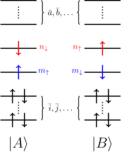
Figure 1: Occupancy of the two reference determinants in TD-CC, $\ket{A}$ and $\ket{B}$, which are related by a global spin-flip transformation.

The model space is thus composed of one singlet (S) and one triplet (T) model wave function:

$$\ket{{}^{\text{S}}\Psi_{0}} =\frac{\ket{A}+\ket{B}}{\sqrt{2}} \ket{{}^{\text{T}}\Psi_{0}} =\frac{\ket{A}-\ket{B}}{\sqrt{2}}$$ (27)

Thus, using Eq. (15) and Eq. (22), the TDCC singlet and triplet wave functions are

$$\ket{{}^{\text{S}}\Psi} =\frac{e^{{}^{A}T}\ket{A}+e^{{}^{B}T}\ket{B}}{\sqrt{2}} \ket{{}^{\text{T}}\Psi} =\frac{e^{{}^{A}T}\ket{A}-e^{{}^{B}T}\ket{B}}{\sqrt{2}}$$ (28)

Because of the spin-flip relation between these model wave functions, the diagonalization of the effective Hamiltonian leads to the following energies for the singlet and triplet states:

$$E^{\text{S}} =\matrixelement*{A}{\hat{H}e^{{}^{A}\hat{T}}}{A}+\matrixelement*{A}{\hat{H}e^{{}^{B}\hat{T}}}{B}$$ (29a)

$$E^{\text{T}} =\matrixelement*{A}{\hat{H}e^{{}^{A}\hat{T}}}{A}-\matrixelement*{A}{\hat{H}e^{{}^{B}\hat{T}}}{B}$$ (29b)

At the TD-CCSD level, the excitation operators are restricted to single and double excitations with respect to their respective references. For example, we have

$$\begin{split}{}^{A}\hat{T}&={}^{A}\hat{T}_{1}+{}^{A}\hat{T}_{2}\\ &=\sum_{ia}{}^{A}t_{i}^{a}\hat{a}^{{\dagger}}\hat{i}+\frac{1}{4}\sum_{ijab}{}^{A}t_{ij}^{ab}\hat{a}^{{\dagger}}\hat{b}^{{\dagger}}\hat{j}\hat{i}\end{split}$$ (30)

with a similar expression for the reference $B$. Note that excitations of the form $t_{{m_{\uparrow}}{n_{\downarrow}}}^{{m_{\downarrow}}{n_{\uparrow}}}\hat{m}^{{\dagger}}_{\downarrow}\hat{n}^{{\dagger}}_{\uparrow}\hat{n}_{\downarrow}\hat{m}_{\uparrow}$, which link $\ket{A}$ to $\ket{B}$, are removed from the summation since the excitations between two determinants of the active space must be discarded.

The ${}^{A}T_{1}$ equations for the reference-dependent amplitudes are

$$\begin{split}{}^{A}Q_{i}^{a}&=\matrixelement*{A_{i}^{a}}{\hat{H}_{N}e^{{}^{A}\hat{T}}}{A}_{\text{c}}-\quantity(\matrixelement*{A_{i}^{a}}{e^{{}^{B}\hat{T}}}{B}H^{\text{eff}}_{BA})_{\text{c}}\\ &=\matrixelement*{A_{i}^{a}}{\hat{H}_{N}e^{{}^{A}\hat{T}}}{A}_{\text{c}}-{{}^{A}}M_{i}^{a}H^{\text{eff}}_{BA}=0\end{split}$$ (31)

while, for the ${}^{A}T_{2}$ equations, we have

$$\begin{split}{}^{A}Q_{ij}^{ab}&=\matrixelement*{A_{ij}^{ab}}{\hat{H}_{N}e^{{}^{A}\hat{T}}}{A}_{\text{c}}-\quantity(\matrixelement*{A_{ij}^{ab}}{e^{{}^{B}\hat{T}}}{B}H^{\text{eff}}_{BA})_{\text{c}}\\ &-P(ij,ab)\quantity[\quantity({{}^{A}}t_{i}^{a}-\hat{R}_{ia}{}^{B}t_{i}^{a})\quantity(\matrixelement*{A_{j}^{b}}{e^{{}^{B}\hat{T}}}{B}H^{\text{eff}}_{BA})_{\text{c}}]\\ &=\matrixelement*{A_{ij}^{ab}}{\hat{H}_{N}e^{{}^{A}\hat{T}}}{A}_{\text{c}}-{{}^{A}}M_{ij}^{ab}H^{\text{eff}}_{BA}=0\end{split}$$ (32)

where $\hat{H}_{N}$ is normal-ordered with respect to $A$, $M_{i}^{a}$, and $M_{ij}^{ab}$ are the so-called renormalization terms, the subscript c indicates that only connected terms are considered, $\hat{R}_{ia}=(1-\delta_{in_{\uparrow}})(1-\delta_{im_{\downarrow}})(1-\delta_{am_{\uparrow}})(1-\delta_{an_{\downarrow}})$, and $P(ij,ab)=1-(i\leftrightarrow j)-(a\leftrightarrow b)+(i\leftrightarrow j)(a\leftrightarrow b)$ is a permutation operator. It is worth noting that one only needs to solve Eqs. (31) and (32) for the reference $A$ since the corresponding amplitudes for $B$ can be easily obtained thanks to the global spin-flip relationship between $A$ and $B$. Further explanations and explicit expressions of each quantity can be found in Refs. Balková and Bartlett, 1992; Szalay and Bartlett, 1994; Lutz et al., 2018.

Furthermore, as explained by Lutz et al., Lutz et al. (2018) only two out of four determinants contribute to the singlet and triplet states in the case of a complete active space (CAS) containing two electrons in two orbitals of different spatial symmetries (as for H2 in a minimal basis set). Therefore, TD-CC is performed on top of a (2,2) complete active space, and the CC single excitation amplitudes between the active orbitals are zero, further simplifying the equations. However, in the case where the active space contains two orbitals of the same spatial symmetry, TD-CC accounts for an incomplete active space. The working equations for both scenarios are presented in the supporting information.

II.6 Derivation of the TD-CCSD Equations

The TD-CCSD equations can be derived by hand using Wick’s theorem or diagrammatic techniques.Kucharski and Bartlett (1991) However, the manual manipulation of a substantial number of equations and indices is highly prone to errors, especially during their implementation in computer software. Fortunately, software solutions are available to streamline this process. Notably, tools such as p^†q by Rubin and DePrince Rubin and DePrince (2021) and wick&d developed by Evangelista Evangelista (2022) can algebraically derive this kind of equations in various contexts.

Let us have a look at Eq. (31) for the ${}^{A}T_{1}$ amplitudes. The first term in the right-hand-side of Eq. (31), $\matrixelement*{A_{i}^{a}}{H_{N}e^{{}^{A}\hat{T}}}{A}_{\text{c}}$, corresponds to the standard term of the $T_{1}$ SRCC equations considered in Eq. (6), with a restriction over the summations in ${}^{A}\hat{T}$. The only new part is the renormalization term, $\quantity(\matrixelement*{A_{i}^{a}}{e^{{}^{B}\hat{T}}}{B}H^{\text{eff}}_{BA})_{\text{c}}$ . To compute the latter term, it is convenient to express each component with respect to a unique reference. For example, the term $H^{\text{eff}}_{BA}=\matrixelement*{B}{\hat{H}e^{{}^{A}\hat{T}}}{A}$ can be obtained by rewriting $\ket{B}$ as an excitation from $\ket{A}$ using Eq. (24), i.e.,

$$\begin{split}\ket{B}&=\hat{n}^{{\dagger}}_{\uparrow}\hat{m}^{{\dagger}}_{\downarrow}\ket{\Phi_{\text{core}}}\\ &=\hat{n}^{{\dagger}}_{\uparrow}\hat{m}^{{\dagger}}_{\downarrow}\hat{m}_{\uparrow}\hat{n}_{\downarrow}\hat{n}^{{\dagger}}_{\downarrow}\hat{m}^{{\dagger}}_{\uparrow}\ket{\Phi_{\text{core}}}\\ &=\hat{n}^{{\dagger}}_{\uparrow}\hat{m}^{{\dagger}}_{\downarrow}\hat{m}_{\uparrow}\hat{n}_{\downarrow}\ket{A}\\ &=\ket{A_{{n_{\downarrow}}{m_{\uparrow}}}^{{n_{\uparrow}}{m_{\downarrow}}}}\end{split}$$ (33)

Thus, the quantity that needs to be evaluated is $\matrixelement*{A_{{n_{\downarrow}}{m_{\uparrow}}}^{{n_{\uparrow}}{m_{\downarrow}}}}{\hat{H}e^{{}^{A}\hat{T}}}{A}$, which is simply one of the SRCC $T_{2}$ equations with additional restrictions over the summations in ${}^{A}\hat{T}$.

The derivation of the second part of the renormalization term, $M_{a}^{i}=\matrixelement*{A_{i}^{a}}{e^{{}^{B}\hat{T}}}{B}$, is a little bit more involved. Due to the presence of $e^{{}^{B}\hat{T}}\ket{B}$, it is easier to express $\bra{A_{i}^{a}}$ as an excitation from the reference $\bra{B}$. To do so, we start by rewriting $\ket{A}$ as an excitation from $\ket{B}$:

$$\begin{split}\ket{A}&=\hat{n}^{{\dagger}}_{\downarrow}\hat{m}^{{\dagger}}_{\uparrow}\ket{\Phi_{\text{core}}}\\ &=\hat{n}^{{\dagger}}_{\downarrow}\hat{m}^{{\dagger}}_{\uparrow}\hat{m}_{\downarrow}\hat{n}_{\uparrow}\hat{n}^{{\dagger}}_{\uparrow}\hat{m}^{{\dagger}}_{\downarrow}\ket{\Phi_{\text{core}}}\\ &=\hat{n}^{{\dagger}}_{\downarrow}\hat{m}^{{\dagger}}_{\uparrow}\hat{m}_{\downarrow}\hat{n}_{\uparrow}\ket{B}\end{split}$$ (34)

which yields

$$\ket{A_{i}^{a}}=\hat{a}^{\dagger}\hat{i}\hat{n}^{{\dagger}}_{\downarrow}\hat{m}^{{\dagger}}_{\uparrow}\hat{m}_{\downarrow}\hat{n}_{\uparrow}\ket{B}$$ (35)

At this stage, a difficulty arises from the fact that $A$ and $B$ do not share the same set of occupied and virtual spin orbitals because of the two unpaired electrons, as shown in Fig. 1 and Eqs. (25a), (26a), (25b), and (26b). To solve this issue, we generate a set of strings of second-quantized operators corresponding to every possible combination of occupancy and spin cases, and apply them to $\bra{B}$:

$$\quantity(\hat{a}^{\dagger}\hat{i}\hat{n}^{{\dagger}}_{\downarrow}\hat{m}^{{\dagger}}_{\uparrow}\hat{m}_{\downarrow}\hat{n}_{\uparrow})^{\dagger}\\ \quad\rightarrow\Bigg{\{}\quantity(\hat{a}^{{\dagger}}_{o}\hat{i}_{o}\hat{n}^{{\dagger}}_{\downarrow}\hat{m}^{{\dagger}}_{\uparrow}\hat{m}_{\downarrow}\hat{n}_{\uparrow})^{\dagger},\quantity(\hat{a}^{{\dagger}}_{v}\hat{i}_{o}\hat{n}^{{\dagger}}_{\downarrow}\hat{m}^{{\dagger}}_{\uparrow}\hat{m}_{\downarrow}\hat{n}_{\uparrow})^{\dagger},\\ \quantity(\hat{a}^{{\dagger}}_{o}\hat{i}_{v}\hat{n}^{{\dagger}}_{\downarrow}\hat{m}^{{\dagger}}_{\uparrow}\hat{m}_{\downarrow}\hat{n}_{\uparrow})^{\dagger},\quantity(\hat{a}^{{\dagger}}_{v}\hat{i}_{v}\hat{n}^{{\dagger}}_{\downarrow}\hat{m}^{{\dagger}}_{\uparrow}\hat{m}_{\downarrow}\hat{n}_{\uparrow})^{\dagger}\Bigg{\}}$$ (36)

where the subscripts $o$ (occupied) and $v$ (virtual) specify the occupancy of the spin orbitals of reference $A$ in the reference $B$. Note that we have not specified the spin of $\phi_{a}$ and $\phi_{i}$ on purpose to reduce the number of terms. Otherwise, by including their spin, each string would lead to four additional terms, that is, $\uparrow\uparrow$, $\uparrow\downarrow$, $\downarrow\uparrow$, and $\downarrow\downarrow$. Subsequently, Wick’s theorem is applied to each of the generated strings. The result is a set of normal-ordered strings of second-quantized operators with Kronecker deltas.

To avoid errors, we have implemented Wick’s theorem for a single string of second-quantized operators in Python. The source code is freely available on github at https://github.com/LCPQ/SimpleWick, and archived in the software heritage database. sim (2023) As a reminder, Wick’s theorem is a technique to rewrite an arbitrary string of second-quantized operators into a sum of normal-order strings. Wick (1950); Crawford and Schaefer (2000); Shavitt and Bartlett (2009) Thus, to evaluate

$$\begin{split}{}^{A}M_{i}^{a}&=\matrixelement*{A_{i}^{a}}{e^{{}^{B}\hat{T}}}{B}\\ &=\matrixelement*{B}{(\hat{a}^{\dagger}\hat{i}\hat{n}^{{\dagger}}_{\downarrow}\hat{m}^{{\dagger}}_{\uparrow}\hat{m}_{\downarrow}\hat{n}_{\uparrow})^{\dagger}e^{{}^{B}\hat{T}}}{B}\end{split}$$ (37)

the string $(\hat{a}^{\dagger}\hat{i}\hat{n}^{{\dagger}}_{\downarrow}\hat{m}^{{\dagger}}_{\uparrow}\hat{m}_{\downarrow}\hat{n}_{\uparrow})^{\dagger}$ is expanded and evaluated as explained above. The resulting strings of normal-ordered second-quantized operators are reordered and fed to p^†q as left operators of the form $\quantity{\hat{i}^{{\dagger}}\hat{j}^{{\dagger}}\cdots\hat{b}\hat{a}}$, using the occupancy definition of Eq. (26a) and  (26b), to be separately evaluated. Schematically, we evaluate terms of the form

$$\matrixelement*{B}{\quantity{\hat{i}^{{\dagger}}\hat{j}^{{\dagger}}\cdots\hat{b}\hat{a}}\ e^{{}^{B}\hat{T}}}{B}$$ (38)

The use of Wick’s theorem allows us to handle the different occupancy cases. To illustrate this, let us consider the first term of Eq. (36) that contributes to ${}^{A}M_{i_{\uparrow}}^{a_{\uparrow}}$. In this case, we have

$$\begin{split}\hat{n}^{{\dagger}}_{\uparrow}\hat{m}^{{\dagger}}_{\downarrow}\hat{m}_{\uparrow}\hat{n}_{\downarrow}\hat{i}^{{\dagger}}_{o\uparrow}\hat{a}_{o\uparrow}&=\quantity{\hat{n}^{{\dagger}}_{\uparrow}\hat{m}^{{\dagger}}_{\downarrow}\hat{m}_{\uparrow}\hat{n}_{\downarrow}\hat{i}^{{\dagger}}_{o\uparrow}\hat{a}_{o\uparrow}}\\ &+\delta_{na}\quantity{\hat{m}^{{\dagger}}_{\downarrow}\hat{m}_{\uparrow}\hat{n}_{\downarrow}\hat{i}^{{\dagger}}_{o\uparrow}}\end{split}$$ (39)

Obviously, the contraction between $a$ and $i$, as well as the contraction between $n$ and $m$, are zero since they correspond to distinct spin orbitals. In addition, it is straightforward to see that the first term of the previous equation yields a zero contribution. Thus, we have

$${}^{A}M_{i_{\uparrow}}^{a_{\uparrow}}=\delta_{na}\matrixelement*{B}{\quantity{\hat{m}^{{\dagger}}_{\downarrow}\hat{i}^{{\dagger}}_{o\uparrow}\hat{m}_{\uparrow}\hat{n}_{\downarrow}}\ e^{{}^{B}\hat{T}}}{B}$$ (40)

which becomes

$$\begin{split}{}^{A}M_{i_{\uparrow}}^{n_{\uparrow}}&={}^{B}t_{m_{\downarrow}i_{\uparrow}}^{n_{\downarrow}m_{\uparrow}}+{}^{B}t_{m_{\downarrow}}^{n_{\downarrow}}{{}^{B}}t_{i_{\uparrow}}^{m_{\uparrow}}\\ &={}^{A}t_{m_{\uparrow}i_{\downarrow}}^{n_{\uparrow}m_{\downarrow}}+{}^{A}t_{m_{\uparrow}}^{n_{\uparrow}}{{}^{A}}t_{i_{\downarrow}}^{m_{\downarrow}}\end{split}$$ (41)

However, because our aim is to evaluate $\quantity(\matrixelement*{A_{i}^{a}}{e^{{}^{B}\hat{T}}}{B}H^{\text{eff}}_{BA})_{\text{c}}$, we must remove the disconnected contributions. To do so, the terms involving at least one cluster amplitude not connected to the effective Hamiltonian, i.e., a cluster amplitude that does not contain any active label, like $m$ or $n$, are excluded. Then, the generated terms are associated with the Kronecker deltas and the signs coming from Wick’s theorem. At this stage, all quantities are related to the reference $B$. We thus perform a global spin-flip transformation on $M_{i}^{a}$ to express the latter quantity with respect to the reference $A$. Finally, the contributions to $M_{i}^{a}$ are generated for computer implementation. A similar procedure is applied to the renormalization term of the ${}^{A}T_{2}$ equations [see Eq. (32)].

To perform all these tasks, we have developed a Python code that interfaces p^†q with the Wick theorem code described above. It enables to generate LaTeX formulas and Fortran code with ease within a jupyter notebook. This code is also freely available on github at https://github.com/LCPQ/Gen_Eq_TDCC, and archived in the software heritage database.gen (2023) For the sake of completeness, the automatically derived formulas related to Eqs. (31) and (32) can be found in the supporting information.

III Computational Details

Most of the molecules and states considered in this paper have been studied in Ref. Kossoski and Loos, 2023 and were originally extracted from the quest database. Véril et al. (2021) The geometries are also taken from the quest database while the state-specific orbitals are the same as those of Ref. Kossoski and Loos, 2023 (see below). We employ the aug-cc-pVDZ basis set for molecules with three or fewer non-hydrogen atoms and the 6-31+G(d) basis otherwise, applying the frozen core approximation (large core for third-row atoms). In the special case of the Be atom, the aug-cc-pVDZ basis set was chosen so as to comply with Ref. Loos et al., 2020. Furthermore, we rely on the same reference values as in Ref. Kossoski and Loos, 2023, which are mainly of CC with singles, doubles, triples, and quadruples (CCSDTQ) or exFCI quality. We consider two new systems, borole and oxalyl fluoride, with geometries optimized at the CC3/aug-cc-pVTZ level of theory following the quest methodology. These are reported in the supporting information.

Our set of excited states comprises 125 singlet, 36 doublet, and 106 triplet states in small- and medium-sized organic compounds, among which there are 9 doubly-excited states. Compared to Ref. Kossoski and Loos, 2023, a few states were removed for reasons detailed below.

In this paper, all the calculations were performed with the quantum package software, Garniron et al. (2019) where CCSD (for both open- and closed-shell systems) and TD-CCSD have been implemented. The calculations were carried out using the $\Delta$CC strategy. Hence, the excitation energies from the ground state were straightforwardly determined as an energy difference between ground and excited states. The ground-state energies were computed with CCSD and ground-state HF orbitals. Different strategies were applied to compute excited states based on their nature. For doubly-excited states, a CCSD calculation was performed on top of a closed-shell doubly-excited determinant. Similarly, for the doublet excited states, a CCSD calculation was performed on top of a singly-excited determinant. Finally, for open-shell singlet and triplet excited states, a TD-CCSD calculation was undertaken using a pair of open-shell singly-excited determinants as the reference.

Concerning the choice of the orbitals, we employ both the ground-state HF and state-specific optimized orbitals. At the HF level, we rely systematically on the restricted HF and restricted open-shell HF (ROHF) formalisms for closed- and open-shell systems, respectively. The state-specific orbitals, extracted from our recent work, Kossoski and Loos (2023) were obtained by optimizing the orbitals for a minimal CSF space using the Newton-Raphson method, also implemented in quantum package. Garniron et al. (2019); Damour et al. (2021) We refer to HF-$\Delta$CCSD as a $\Delta$CCSD calculation where ground-state HF orbitals have been considered for both ground and excited states, while oo-$\Delta$CCSD denotes a $\Delta$CCSD calculation that employs HF orbitals for the ground state and state-specific optimized orbitals for the excited state. For HF-$\Delta$CCSD, the excited-state calculations were performed by changing the orbital occupancy to match with the excited-state dominant determinant obtained from a prior EOM-CCSD calculation. For oo-$\Delta$CCSD, the excited-state calculations were done for a non-Aufbau single CSF reference for which the orbitals were optimized. It is important to note that the orbitals in oo-$\Delta$CCSD are optimized for a single CSF wave function. In other words, they do not minimize the CCSD energy as in orbital-optimized CCSD. Sherrill et al. (1998); Krylov et al. (1998); Krylov, Sherrill, and Head-Gordon (2000); Bozkaya et al. (2011)

In the statistical analysis presented below, we report the usual indicators: the mean signed error (MSE), the mean absolute error (MAE), the root-mean-square error (RMSE), and the standard deviation of the errors (SDE). For the sake of completeness, the raw data associated with each figure and table, in addition to the total and excitation energies computed at the different levels of theory are reported in the supporting information.

IV Results and discussion

IV.1 Doubly-excited states

For the doubly-excited states, we limited our focus to a small subset of 9 molecules, including the 6 listed in Ref. 84 complemented with borole, oxalyl fluoride, and tetrazine. Other molecules such as C2 and C3 are excluded from this study since they require consideration of more than one closed-shell determinant to accurately describe their doubly-excited states. Kossoski and Loos (2023) This requirement becomes evident when examining the coefficients of their CI wave function. Additionally, we restrict ourselves to “genuine” double excitations only, which have a small contribution from the single excitations (see the $\%T_{1}$ values in Table 1) and are hence reasonably well described by a single closed-shell determinant. Transitions with a dominant single excitation character, yet a significant partial double excitation contribution (large $\%T_{1}$ values), such as the famous $2{}^{1}A_{g}$ dark state of butadiene, Saha, Ehara, and Nakatsuji (2006); Watson and Chan (2012); Shu and Truhlar (2017); Barca, Gilbert, and Gill (2018a); Loos et al. (2019); do Casal et al. (2023) are treated as single excitations using TD-CCSD (see Sec. IV.3). Most of the reference data for these transitions have been extracted from Ref. Loos et al., 2019.

The results for each system are represented in Fig. 2 and are also collected in Table 1, where we further report the $\Delta$SCF results and the value of $\%T_{1}$ computed at the CC3/aug-cc-pVTZ level. We do not consider EOM-CCSD due to the very poor quality of the results. Indeed, it is well known that, at this level of theory, some of the doubly-excited states are overshooted by several eV. For the doubly-excited states, we do not perform a statistical analysis due to the limited number of states.

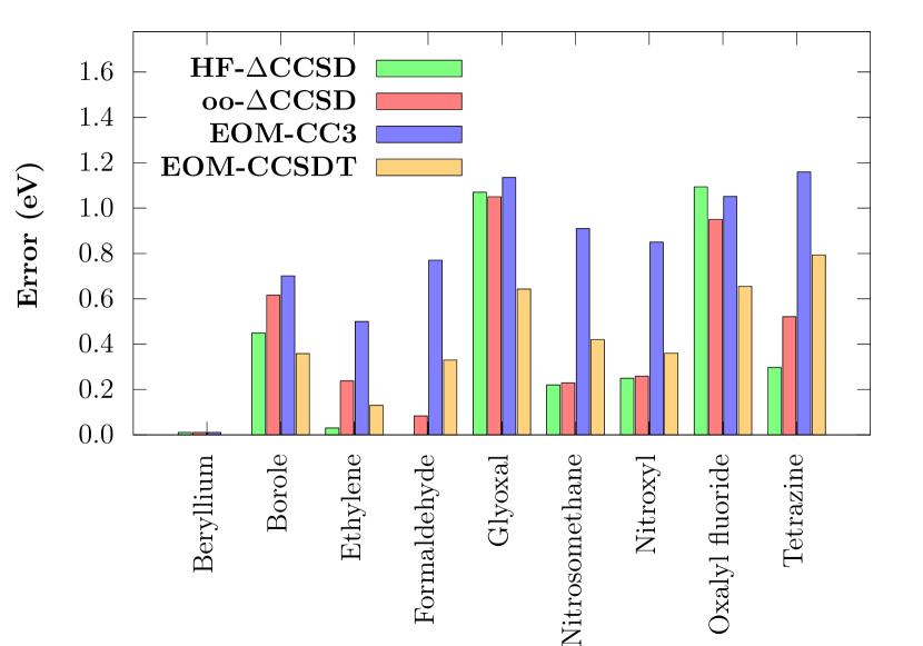
Figure 2: Errors in the excitation energies (with respect to the reference values) of doubly-excited states, computed at various levels of theory. See Table 1 for the raw data.

Table 1: Excitation energies associated with the doubly-excited states calculated at various levels of theory. The error with respect to the reference value is reported in parentheses.

		Excitation energies $\mathrm{eV}$
Molecule	$\%T_{1}$	Ref.	$\Delta$SCF	HF-$\Delta$CCSD	oo-$\Delta$CCSD	EOM-CC3	EOM-CCSDT
Beryllium	$29$	$7.22$	7.86(+0.64)	7.23(+0.01)	7.23(+0.01)	7.23(+0.01)	7.22(+0.00)
Borole	$20$	$4.71$	5.70(+0.99)	5.16(+0.45)	5.33(+0.62)	5.41(+0.70)	5.07(+0.36)
Ethylene	$20$	$13.07$	13.54(+0.47)	13.10(+0.03)	13.31(+0.24)	13.57(+0.50)	13.20(+0.13)
Formaldehyde	$5$	$10.45$	10.83(+0.38)		10.53(+0.08)	11.22(+0.77)	10.78(+0.33)
Glyoxal	$0$	$5.60$	10.50(+4.90)	6.67(+1.07)	6.55(+0.95)	6.74(+1.14)	6.24(+0.64)
Nitrosomethane	$3$	$4.84$	4.96(+0.12)	5.06(+0.22)	5.07(+0.23)	5.75(+0.91)	5.26(+0.42)
Nitroxyl	$0$	$4.40$	4.57(+0.17)	4.65(+0.25)	4.66(+0.26)	5.25(+0.85)	4.76(+0.36)
Oxalyl fluoride	$2$	$9.21$	12.57(+3.37)	10.30(+1.09)	10.16(+0.95)	10.26(+1.05)	9.86(+0.66)
Tetrazine	$1$	$5.06$	7.77(+2.71)	5.36(+0.30)	5.58(+0.52)	6.22(+1.16)	5.86(+0.79)

Interestingly, we found that HF-$\Delta$CCSD generally yields similar results to those of oo-$\Delta$CCSD, with the exception of formaldehyde, for which we were not able to locate the state of interest with HF-$\Delta$CCSD. This result reveals a limited effect of mean-field orbital optimization for $\Delta$CCSD calculations. It is also worth noticing that both HF-$\Delta$CCSD and oo-$\Delta$CCSD systematically overestimate the excitation energies, hinting at the importance of the missing contributions from higher excitations (see below).

Glyoxal and oxalyl fluoride exhibit the largest errors of our set (around $1\text{\,}\mathrm{eV}$), with both HF-$\Delta$CCSD and oo-$\Delta$CCSD. Based on SCI calculations, for both molecules and with both methods, we found that the CI coefficient associated with the reference determinant of the excited state is large ($\approx 0.8$). One possible explanation for the observed discrepancy lies in the existence of a second doubly-excited determinant, relative to both the HF and the reference determinant, which carries a substantial weight in the wave function ($\approx 0.2$). Indeed, for glyoxal, including this second determinant in the reference space leads to improved results in state-specific CI with singles and doubles ($\Delta$CISD) calculations. Kossoski and Loos (2023) It is also interesting to notice that the presence of singly-excited determinants with somewhat larger coefficients (up to $\approx 0.3$) is problematic, based on the smaller errors we observe in the other doubly-excited states. Therefore, the inaccuracies for glyoxal and oxalyl fluoride may originate from the fact that important single and double excitations accessed from the second doubly-excited determinant are not accounted for, which would appear as triple and quadruple excitations with respect to the reference determinant, and are thus lacking in the $\Delta$CCSD calculations. This also explains the systematically overestimated excitation energies.

When compared to standard EOM-CC methods, the $\Delta$CCSD approach demonstrates its superiority for the doubly-excited states surveyed here, outperforming EOM-CC3 and even EOM-CCSDT in some cases. However, $\Delta$CCSD becomes less accurate when dealing with systems possessing several doubly-excited determinants with significant weights, as discussed above for glyoxal and oxalyl fluoride.

IV.2 Doublet-doublet transitions

We included all the radical doublets from Ref. Kossoski and Loos, 2023, except for 11 states (outlined below), making a total of 36 states in the present set. The reference data for these molecules have been extracted from Ref. Loos et al., 2020. We did not consider the four states of nitromethyl, since their assignment is particularly challenging due to the significant deviations observed between EOM-CCSD and EOM-CCSDT. We also excluded one state of BeH as the two states of interest share the same dominant determinant and one state of BeF, for which we did not manage to converge the orbital optimization. Moreover, HF-$\Delta$CCSD leads to very large errors for two states of CH, as they need two open-shell determinants to be qualitatively described. Kossoski and Loos (2023) Hence, they have also been discarded. Finally, we did not consider one of the states of vinyl and the two states of OH which need three determinants with three unpaired electrons to be described. Kossoski and Loos (2023) The detailed results for all the states can be found in the supporting information.

Our set of 36 doublet-doublet transitions should be large enough to render reasonable statistics. The distribution of errors with respect to accurate reference values, as obtained with EOM-CCSD, HF-$\Delta$CCSD, and oo-$\Delta$CCSD, is illustrated in Fig. 3, whereas the associated statistical measures are reported in Table 2. When compared to EOM-CCSD, the distribution of errors for HF-$\Delta$CCSD and oo-$\Delta$CCSD appears to be less sharp, leading to slightly worse statistics. Indeed, the distributions are similar for HF-$\Delta$CCSD and oo-$\Delta$CCSD, with comparable MAEs ($0.09\text{\,}\mathrm{eV}0.10\text{\,}\mathrm{eV}$), both underperforming EOM-CCSD, which has a MAE of $0.07\text{\,}\mathrm{eV}$. The same can be concluded from the RMSEs and SDEs. Surprisingly, in contrast to HF-$\Delta$CCSD, which has a near-zero MSE, oo-$\Delta$CCSD has the same slightly positive MSE ($0.05\text{\,}\mathrm{eV}$) as EOM-CCSD. Thus, the use of optimized orbitals instead of HF ground-state orbitals does not improve the overall accuracy. On the contrary, the MAE, RMSE, and SDE are slightly larger (by $0.01\text{\,}\mathrm{eV}$ or $0.02\text{\,}\mathrm{eV}$) when optimized orbitals are employed, which could be a statistical artifact though. Overall, the accuracy of $\Delta$CCSD for doublet-doublet transitions is only marginally worse compared to EOM-CCSD.

We further notice that oo-$\Delta$CCSD is more accurate than the $\Delta$CISD calculations reported in Ref. Kossoski and Loos, 2023, with respective MAEs of $0.10\text{\,}\mathrm{eV}$ and $0.16\text{\,}\mathrm{eV}$. Since both methods employ the same set of state-specific orbitals, reference wave function, and excitation manifold (singles and doubles), the superior performance of oo-$\Delta$CCSD can be attributed to the inclusion of higher-order excitations accessed through the connected terms of CC.

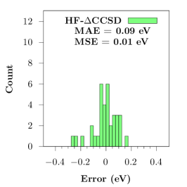
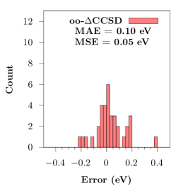
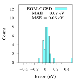
Figure 3: Histograms of the error in excitation energies (with respect to the reference values) computed at the HF-$\Delta$CCSD (left), oo-$\Delta$CCSD (center), and EOM-CCSD (right) levels for doublet-doublet transitions.

Table 2: Statistical indicators associated with the errors in doublet-doublet transitions computed at the EOM-CCSD, HF-$\Delta$CCSD, and oo-$\Delta$CCSD levels. All values are in $\mathrm{eV}$.

Method	# states	MAE	MSE	RMSE	SDE
EOM-CCSD	$36$	$0.07$	$0.05$	$0.13$	$0.12$
HF-$\Delta$CCSD	$36$	$0.09$	$0.01$	$0.15$	$0.15$
oo-$\Delta$CCSD	$36$	$0.10$	$0.05$	$0.17$	$0.16$

IV.3 Open-shell singly-excited states

Let us now focus on the performance of $\Delta$CCSD for open-shell singly-excited states of closed-shell systems. Out of the 237 states considered, two could not be targeted with our protocol for HF-$\Delta$CCSD calculations, since their dominant determinants are the same as those of a lower-lying excited state. In addition, HF-TDCC calculations did not converge for four other states, making a total of 231 converged states. All the results are available in the supporting information, with the above-mentioned problematic cases highlighted in magenta.

The distribution of errors in the excitation energy for the three methods assessed here is depicted in Fig. 4, and the corresponding statistical analysis is reported in Table 3. For the full set of singly-excited states, HF-$\Delta$CCSD and oo-$\Delta$CCSD share a near-zero MSE ($0.02\text{\,}\mathrm{eV}$), and a comparable accuracy, with a small advantage for the latter (MAE of $0.15\text{\,}\mathrm{eV}$ against $0.17\text{\,}\mathrm{eV}$). oo-$\Delta$CCSD produces fewer outliers than HF-$\Delta$CCSD, which is clear from their corresponding RMSEs, of $0.27\text{\,}\mathrm{eV}$ and $0.35\text{\,}\mathrm{eV}$. oo-$\Delta$CCSD is also more consistent than HF-$\Delta$CCSD, having SDEs of $0.26\text{\,}\mathrm{eV}$ and $0.35\text{\,}\mathrm{eV}$. Orbital optimization enhances the description of singly-excited states, particularly for those poorly characterized by HF-$\Delta$CCSD, providing a more accurate overall representation. Both methods compare unfavorably with EOM-CCSD, however, which has a considerably smaller MAE ($0.08\text{\,}\mathrm{eV}$), RMSE and SDE, although it shows a somewhat positive MSE ($0.05\text{\,}\mathrm{eV}$). Compared to the closer performances of HF-$\Delta$CCSD, oo-$\Delta$CCSD, and EOM-CCSD for doublet-doublet transitions, the larger discrepancies for singly-excited states are noteworthy.

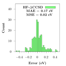
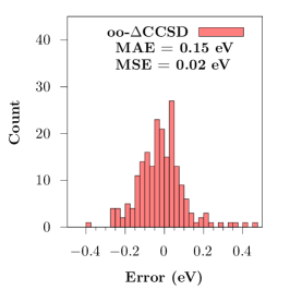
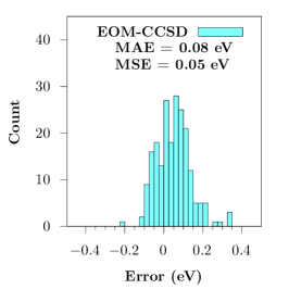
Figure 4: Histograms of the error in excitation energies (with respect to the reference values) at the HF-$\Delta$CCSD (left), oo-$\Delta$CCSD (center), and EOM-CCSD (right) levels, for open-shell singly-excited states.

Table 3: Statistical results associated with the errors in excitation energies (with respect to the reference values) for the singlet and triplet singly-excited states computed with EOM-CCSD, HF-$\Delta$CCSD, and oo-$\Delta$CCSD. Values in parenthesis are obtained by discarding 19 states having four dominant determinants with the exact same weight in the EOM-CCSD vector, which are all $\pi\pi^{*}$ valence excitations involving degenerate orbitals. All values are in $\mathrm{eV}$.

Method	Character	# states	MAE	MSE	RMSE	SDE
EOM-CCSD	All	231 (212)	0.08 (0.09)	0.05 ( 0.05)	0.13 (0.13)	0.12 (0.12)
	Singlet	125 (116)	0.10 (0.10)	0.09 ( 0.09)	0.13 (0.13)	0.09 (0.10)
	Triplet	106 ( 96)	0.07 (0.06)	-0.01 (-0.00)	0.12 (0.13)	0.12 (0.13)
	Valence	152 (133)	0.09 (0.09)	0.04 ( 0.05)	0.14 (0.14)	0.13 (0.14)
	Rydberg	79 ( 79)	0.08 (0.08)	0.05 ( 0.05)	0.09 (0.09)	0.08 (0.08)
HF-$\Delta$CCSD	All	231 (212)	0.17 (0.13)	0.02 (-0.01)	0.35 (0.28)	0.35 (0.28)
	Singlet	125 (116)	0.17 (0.11)	0.03 (-0.02)	0.38 (0.29)	0.38 (0.29)
	Triplet	106 ( 96)	0.18 (0.15)	-0.01 (-0.01)	0.32 (0.28)	0.32 (0.28)
	Valence	152 (133)	0.20 (0.14)	0.06 ( 0.02)	0.36 (0.24)	0.35 (0.24)
	Rydberg	79 ( 79)	0.12 (0.12)	-0.07 (-0.07)	0.34 (0.34)	0.33 (0.33)
oo-$\Delta$CCSD	All	231 (212)	0.15 (0.12)	0.02 (-0.01)	0.27 (0.20)	0.26 (0.20)
	Singlet	125 (116)	0.15 (0.11)	0.04 ( 0.00)	0.29 (0.18)	0.29 (0.18)
	Triplet	106 ( 96)	0.13 (0.12)	-0.00 (-0.03)	0.23 (0.22)	0.23 (0.22)
	Valence	152 (133)	0.17 (0.13)	0.04 (-0.02)	0.31 (0.22)	0.31 (0.22)
	Rydberg	79 ( 79)	0.09 (0.09)	-0.01 (-0.01)	0.15 (0.15)	0.15 (0.15)

HF-$\Delta$CCSD and oo-$\Delta$CCSD show a substantial number of absolute errors exceeding $0.2\text{\,}\mathrm{eV}$, in contrast to EOM-CCSD. This significantly deteriorates the statistics of these methods, since 19 and 15 states, respectively, have errors above $0.5\text{\,}\mathrm{eV}$. For EOM-CCSD, this happens for 2 states only. Understanding the reasons behind the inaccuracy of HF-$\Delta$CCSD and oo-$\Delta$CCSD for these specific cases is important. TD-CC is expected to perform well for states described by a single CSF; however, it is less effective for excited states that exhibit a pronounced multiconfigurational character, which would necessitate additional CSFs. To evaluate its performance for the former type of states only, we excluded 19 states having four dominant determinants with the exact same weight in the EOM-CCSD vector, which are indicated in red in the supporting information. These transitions involve degenerate $\pi$/$\pi^{*}$ orbitals and would require at least two CSFs to be qualitatively described. The associated statistics excluding results from this subset of singly-excited states are shown in parenthesis in Table 3. By discarding these multiconfigurational excited states, the statistics for both HF-$\Delta$CCSD and oo-$\Delta$CCSD are systematically improved. In particular, the MAE of HF-$\Delta$CCSD decreases from $0.17\text{\,}\mathrm{eV}$ to $0.13\text{\,}\mathrm{eV}$, whereas that of oo-$\Delta$CCSD decreases from $0.15\text{\,}\mathrm{eV}$ to $0.12\text{\,}\mathrm{eV}$. The accuracy of $\Delta$CCSD methods thus approaches that of EOM-CCSD, which remains almost unaltered (with a slightly larger MAE of $0.09\text{\,}\mathrm{eV}$) in this case. Moreover, the comparable improvement for both HF-$\Delta$CCSD and oo-$\Delta$CCSD suggests that orbital optimization is overall equally helpful for the single and multiconfigurational excited states.

Further examining the EOM-CCSD eigenvectors shows that HF-$\Delta$CCSD and oo-$\Delta$CCSD usually deliver larger errors for states with important contributions coming from several determinants, especially when these determinants are doubly excited with respect to the two determinants considered for the TD-CC calculation. From this last point, the magnitude of the errors becomes less surprising, since we perform all single and double excitations on top of a two-determinant reference. For instance, by further discarding the three excited states having the largest contribution from doubly-excited determinants with respect to those used in TD-CC (based on the EOM-CCSD vector), namely the ${1}^{3}A_{1}$ state of cyclopentadiene, the ${2}^{1}B_{2}$ state of cyclopropenone, and the ${1}^{3}A_{g}$ state of butadiene, highlighted in yellow in the supporting information, one obtains even smaller MAEs for HF-$\Delta$CCSD and oo-$\Delta$CCSD, of $0.12\text{\,}\mathrm{eV}$ and $0.11\text{\,}\mathrm{eV}$, whereas the MAE of EOM-CCSD remains unchanged at $0.09\text{\,}\mathrm{eV}$. Clearly, the performance of $\Delta$CC methods, TD-CC in particular, approaches the one of EOM-CCSD for states dominated by a single open-shell CSF but deteriorates as the multiconfigurational character of the excited states becomes more pronounced.

Another important aspect concerns the accuracy of the $\Delta$CCSD methods with respect to the nature of the excitation. As can be seen from Table 3, EOM-CCSD suffers from significant differences in its MAE and MSE when comparing singlet and triplet states. This behavior may be attributed to variations in the $\%T_{1}$ values, as triplets generally have typically much higher $\%T_{1}$ than singlets. Véril et al. (2021) Thus, it is reasonable to expect a more favorable treatment of triplets with EOM-CCSD. On the other hand, HF-$\Delta$CCSD and oo-$\Delta$CCSD share a similar MAE and MSE, meaning that $\Delta$CCSD demonstrates greater consistency in the treatment of singlet and triplet states. When disregarding the more problematic multiconfigurational excited states, the small gap between the MAE for singlets and triplets is preserved in the case of oo-$\Delta$CCSD, but actually increases for HF-$\Delta$CCSD, becoming comparable to that of EOM-CCSD.

When looking at the statistics for valence and Rydberg states, $\Delta$CCSD seems to be less consistent than EOM-CCSD. While it provides a better treatment of the Rydberg states, the description of the valence ones is less satisfactory. The same trend is observed in EOM-CCSD, though to a lesser degree. A closer examination of the statistics reveals that the issue primarily arises from the $\pi\pi^{*}$ transitions, which are less accurately described than the other valence excitations (the results are shown in the supporting information). However, the gap between valence and Rydberg transitions encountered for $\Delta$CCSD is considerably reduced once the 19 multiconfigurational excited states described above are discarded (see Table 3). In fact, EOM-CCSD also exhibits a poorer description of $\pi\pi^{*}$ transitions, albeit by a smaller margin.

oo-$\Delta$CCSD is also more accurate than $\Delta$CISD Kossoski and Loos (2023) for the singly-excited states, with respective MAEs of $0.10\text{\,}\mathrm{eV}$ and $0.16\text{\,}\mathrm{eV}$, respectively. To have a fair comparison, these MAEs were computed by considering the subset of 203 excited states described by a single CSF reference in Ref. Kossoski and Loos, 2023. In this case, the two sets of calculations only differ by the connectedness of CC, which implicitly accounts for higher-order excitations. The $0.06\text{\,}\mathrm{eV}$ improvement equals the one found for the doublet-doublet transitions.

V Concluding Remarks

In this work, we studied the use of state-specific CCSD approaches to compute vertical excitation energies and compare them with the standard EOM-CCSD approach. Thanks to the present implementation of TD-CCSD and CCSD based on a non-Aufbau determinant, we conducted a substantial number of calculations on various types of excited states to assess the performance of these state-specific approaches. Our investigation began with closed-shell doubly-excited states, where $\Delta$CCSD is known to work quite well (see, for example, Ref. Lee, Small, and Head-Gordon, 2019). Next, we extended our exploration to doublet-doublet transitions in radicals, for which both ground and excited states are generally well-described by a single (open-shell) Slater determinant. Finally, we inspected more traditional single excitation processes leading to both singlet and triplet excited states using TD-CCSD, which allows us to perform CCSD calculations on top of a single CSF.

In the context of doubly-excited states, $\Delta$CCSD produces results that are comparable to EOM-CCSDT and significantly more accurate than EOM-CCSD. This is an expected outcome because, by construction, at the EOM-CCSD level, the similarity-transformed Hamiltonian only contains the reference determinant in addition to its single and double excitations. This level of description is simply insufficient to accurately describe the genuine doubly-excited states considered here, which require the inclusion of triples and quadruples to be properly correlated.

The results for the other kinds of states yielded somewhat unexpected outcomes. Indeed, because EOM-CCSD is biased toward the ground state, one might expect improved results by starting from a more suitable, state-specific reference. However, our findings did not indicate any substantial improvement with the state-specific approaches followed here. Additionally, employing optimized orbitals for the reference CSF in oo-$\Delta$CCSD did not lead to a significant improvement in the accuracy when compared to HF-$\Delta$CCSD. This observation may be attributed to the fact that our optimized orbitals minimize the energy associated with the reference CSF but do not minimize the corresponding CCSD energy. Nonetheless, it is noteworthy that, for most of the states investigated here, $\Delta$CCSD did not significantly deteriorate the quality of the doublet states as compared to EOM-CCSD, with a small MAE increase from $0.07\text{\,}\mathrm{eV}$ to $0.10\text{\,}\mathrm{eV}$ (for oo-$\Delta$CCSD).

Finally, for singlet and triplet singly-excited states, $\Delta$CCSD produced twice larger errors (MAEs of $0.15\text{\,}\mathrm{eV}0.17\text{\,}\mathrm{eV}$) than EOM-CCSD (MAE of $0.08\text{\,}\mathrm{eV}$). Excited states with a strong multiconfigurational character are less well described with $\Delta$CCSD approaches, which could be expected. Ignoring these states from the statistics reduces the MAEs by $0.03\text{\,}\mathrm{eV}0.04\text{\,}\mathrm{eV}$, which is however not enough to match the systematically very good performance of EOM-CCSD for the states considered here. We also found that state-specifically optimizing the orbitals leads to a small but statistically significant improvement for this class of excitation. On the bright side, $\Delta$CCSD enables a more consistent treatment of singlet and triplet states than EOM-CCSD. Consequently, while $\Delta$CCSD may not surpass EOM-CCSD for single-reference singly-excited states, it may offer an attractive alternative for achieving a more consistent treatment of excited states of different spin multiplicities, which remains to be explored. State-specifically optimizing the ground- and excited-state orbitals at the CCSD level is another avenue one should explore but is left as a future work.

In comparison to standard multiconfigurational methods, such as CASPT2 or NEVPT2, $\Delta$CCSD demonstrates interesting performance. While the former methods typically yield excitation energy errors in the range of $0.1\text{\,}\mathrm{eV}0.2\text{\,}\mathrm{eV}$Schapiro, Sivalingam, and Neese (2013); Sarkar et al. (2022); Boggio-Pasqua, Jacquemin, and Loos (2022); Battaglia, Fdez. Galván, and Lindh (2023) and involve a computational complexity that grows factorially with the size of the active space, $\Delta$CCSD provides excitation energies with errors between $0.10\text{\,}\mathrm{eV}$ and $0.15\text{\,}\mathrm{eV}$ at a computational cost scaling polynomially with the system size. Thus, $\Delta$CCSD may emerge as an appealing alternative for accurately describing excitations that demand a large active space in multiconfigurational methods.

In addition to the classes of excited states considered in the present benchmark study, there remains the unexplored class of charge-transfer states, which could be of particular interest for future assessments of $\Delta$CCSD. Kozma et al. (2020); Loos et al. (2021) In this case, orbital relaxation is known to be crucial, Schmerwitz, Levi, and Jónsson (2023) and thus $\Delta$CCSD may be expected to outperform EOM-CCSD. In addition, the present analysis mainly focused on small- and medium-sized molecules. Future investigations could extend this study to larger systems. Indeed, the quality of EOM-CCSD deteriorates with increasing system size and becomes less accurate than EOM-CC2 for large systems. Loos and Jacquemin (2021) It remains to be seen whether this observation holds true within the state-specific formalism.

Supporting Information

See the supporting information for the geometries of borole and oxalyl fluoride, further statistical measures, the TD-CCSD equations, the raw data associated with each figure and table, in addition to the energies at different levels of theory in the considered basis sets.