Evidence for transit-timing variations of the 11 Myr exoplanet TOI-1227 b

TOI-1227 b is an 11 Myr old validated transiting planet in the middle of its contraction phase, with a current radius of 0.85 $\mathrm{R}_{\rm J}$. It orbits a low-mass pre-main sequence star (0.170 $M_{\odot}$, 0.56 $R_{\odot}$) every 27.4 days. The magnetic activity of its young host star induces radial velocity jitter and prevents good measurements of the planetary mass. We gathered additional transit observations of TOI-1227 b with space- and ground-based telescopes, and we detected highly significant transit-timing variations (TTVs). Their amplitude is about 40 minutes and their dominant timescale is longer than 3.7 years. Their most probable origin is dynamical interactions with additional planets in the system. We modeled the TTVs with inner and outer perturbers near first and second order resonances; several orbital configurations provide an acceptable fit. More data are needed to determine the actual orbital configuration and eventually measure the planetary masses. These TTVs and an updated transit chromaticity analysis reinforce the evidence that TOI-1227 b is a planet.

1 Introduction

Young planets offer unique insight into the early physical processes that shape planetary systems, such as the post-formation cooling and contraction of the planets (Vazan et al. 2013; Mordasini et al. 2012; Linder et al. 2019), their orbital evolution (Matsumura et al. 2010; Bolmont et al. 2017), and the influence of stellar radiation on planetary evolution (Lopez et al. 2012; Owen & Wu 2017; Kubyshkina et al. 2020). In particular, very young resonant multi-planetary systems allow the resonance configuration to be observed as it formed in the protoplanetary disk (Teyssandier & Libert 2020), before tidal dissipation erases the pristine configuration (Papaloizou & Terquem 2010; Delisle & Laskar 2014).

The planets of AU Mic (Plavchan et al. 2020; Cale et al. 2021) and V1298 Tau b and e (David et al. 2019; Suárez Mascareño et al. 2021; Finociety et al. 2023) unfortunately remain the only planets with both mass and radius measurements for ages below 50 Myr. TOI-1227 b (Mann et al. 2022) is, alongside K2-33 (David et al. 2016; Mann et al. 2016), the youngest transiting planet known to date, with an age of just $11\pm 2$ Myr (estimated due to its membership to the Musca group, Mann et al. 2022). The planet orbits a very low-mass pre-main sequence star ($0.170\pm 0.015$ $M_{\odot}$, $0.56\pm 0.03$ $R_{\odot}$) every 27.4 days, which makes TOI-1227 b the youngest transiting planet around the least massive star known today.

Young planets are key for theory of planet formation and evolution since they provide direct observational constraints just at the interface of the two stages. Such constraints will be crucial, for instance, to shed light on the current debate about the origin and composition of super-Earths and mini-Neptunes, where some studies propose a solely post-formation atmospheric-loss explanation (Owen & Wu 2017), while others highlight the importance of planet formation in producing the two populations of planets (Venturini et al. 2020). In addition, different evolutionary processes such as photoevaporation (Owen & Wu 2017) and core-powered mass loss (Gupta & Schlichting 2019) yield equal outputs after gigayears of evolution, but they act on different timescales when scrutinizing at the $\sim$10-100 Myr level. Furthermore, several physical parameters affect the size of a planet over time, such as the core and envelope mass and composition (Mordasini 2020; Dorn et al. 2017), the presence of compositional gradients (Vazan et al. 2013), internal luminosity (Guillot 2010), the extension of convective and radiative regions (Haldemann et al. 2023), and the extreme-ultraviolet (XUV) environment (Kubyshkina et al. 2020); however, their distinctive imprint fades for mature, gigayear-old planets. On the contrary, the size of young planets is much more sensitive to these model assumptions (Mordasini et al. 2012; Vazan et al. 2013; Müller et al. 2020), which suggest the possibility of disentangling among them when observing planets that just emerged from the protoplanetary disk.

TOI-1227 b has a measured size of 0.85 $\mathrm{R}_{\rm J}$, and its mass is not known. Planet evolution models indicate that in order to match the planet size at its inferred age, the planet mass could range between approximately 5 and 50 $\mathrm{M_{E}}$, depending on different model assumptions (Mordasini et al. 2012; Linder et al. 2019; Mann et al. 2022). The planet is believed to be halfway through its contraction phase, and it is expected to mature into a planet of roughly Neptune size when reaching an age of approximately a gigayear (Mann et al. 2022). Determining the planet’s mass is key to set proper constraints on the model assumptions mentioned above (otherwise the unknown mass becomes a confounding factor). Radial velocity measurements are very challenging for this target due to the stellar activity. The starspots on fast-rotating young stars do indeed induce large apparent radial velocity variations (e.g., Donati et al. 2023), blurring any planetary signal. Because of this, only an upper mass limit of $\simeq$0.5 $\mathrm{M}_{\rm J}$ could be reported from past radial velocity campaigns (Mann et al. 2022). Due to the difficulties entailed in obtaining radial velocities for a target of these characteristics, transit-timing variations (TTVs, Agol et al. 2005; Holman & Murray 2005) from dynamical interactions offer an alternative and promising path to constrain the planet mass, not only for TOI-1227 b, but in general for any young multi-planetary system (Martioli et al. 2021).

We observed additional transits of TOI-1227 b and detected TTVs, which suggest that the system contains at least one additional planet. The article is organized as follows: We present the new transit photometry of TOI-1227 b in Sect. 2, we explain how we derived the transit timings in Sect. 3 and modeled them in Sect. 4. Finally, in Sect. 5 we discuss the results of our work.

2 Observations

We first collected the Transiting Exoplanet Survey Satellite (TESS, Ricker et al. 2015) and ground-based transit photometry observations presented in Mann et al. (2022). To those literature data, we added new photometry gathered since by TESS, as well as follow-up ground-based observations with Antarctica Search for Transiting ExoPlanets (ASTEP), Exoplanets in Transits and their Atmospheres (ExTrA), Search for habitable Planets EClipsing ULtra-cOOl Stars (SPECULOOS-South), and TRAnsiting Planets and PlanetesImals Small Telescope (TRAPPIST-South). Table 1 summarizes all transit observations used in this work, and we detail the new observations by telescope below.

Table 1: Log of transit observations.

Epoch	Mid-transit date	Telescope	Band	Exposure time	Coverage	Source
	YYYY-MM-DD (UT)			[s]
0	2019-05-13	TESS s11	TESS	120	Full	Mann et al. (2022)
1	2019-06-10	TESS s12	TESS	120	Full	Mann et al. (2022)
9	2020-01-15	SOAR	i’	120	Full	Mann et al. (2022)
13	2020-05-03	LCOGT-SSO	i’	200	Partial	Mann et al. (2022)
16	2020-07-24	LCOGT-SAAO	r’, zS	200	Partial	Mann et al. (2022)
25	2021-03-28	SOAR	g’	120	Partial	Mann et al. (2022)
26	2021-04-24	LCOGT-SSO	zS	210	Partial	Mann et al. (2022)
26	2021-04-24	ASTEP	ASTEP	200	Partial	Mann et al. (2022)
27	2021-05-21	TESS s38	TESS	120	Full	Mann et al. (2022)
28	2021-06-18	LCOGT-CTIO	g’	300	Partial	Mann et al. (2022)
28	2021-06-18	ExTrA T23	ExTrA	60	Partial	This work
39	2022-04-15	TRAPPIST-South	I+z	180	Full	This work
39	2022-04-15	ExTrA T23	ExTrA	60	Partial	This work
40	2022-05-12	ExTrA T3	ExTrA	60	Partial	This work
51	2023-03-09	ExTrA T123	ExTrA	60	Partial	This work
53	2023-05-03	TESS s64	TESS	120	Full	This work
53	2023-05-03	SPECULOOS-Io	z’	21	Full	This work
53	2023-05-03	ExTrA T123	ExTrA	60	Full	This work
54	2023-05-30	TESS s65	TESS	120	Full	This work
54	2023-05-30	ASTEP	ASTEP+ Red	200	Full	This work
55	2023-06-26	ASTEP	ASTEP+ Red	200	Full	This work
57	2023-08-20	ASTEP	ASTEP+ Red	200	Partial	This work

2.1 ASTEP

The ASTEP is a 0.4-m telescope equipped with a Wynne Newtonian coma corrector, located at Dome C on the east Antarctic plateau (Guillot et al. 2015; Mékarnia et al. 2016). Until December 2021, it was equipped with a 4k × 4k front-illuminated FLI Proline KAF-16801E CCD with an image scale of $0.93\arcsec\rm{pixel}^{-1}$ resulting in a $1^{\circ}\times 1^{\circ}$ corrected field of view. The focal instrument dichroic plate split the beam into a blue wavelength channel for guiding, and a non-filtered red science channel roughly matching an $Rc$ transmission curve (Abe et al. 2013). In January 2022, the focal box was replaced with a new one with two high sensitivity cameras including an Andor iKon-L936 at red wavelengths. The image scale is $1.39\arcsec\rm{pixel}^{-1}$ with a transmission curve centered on 850$\pm$138 nm (Schmider et al. 2022). The telescope is automated or remotely operated when needed. Due to the extremely low data transmission rate at the Concordia station, the data are processed on-site using IDL (Mékarnia et al. 2016) and Python (Dransfield et al. 2022) aperture photometry pipelines. The raw light curves of up to 1 000 stars in the field are transferred to Europe on a server in Rome, Italy, and they are then available for deeper analysis.

Four observations of TOI-1227 b were carried out with ASTEP, all under clear sky conditions with winds between 2 and 5 ms^-1 and a temperature ranging between $-$65 and $-$70^∘C. An egress was observed on 24 April 2021 with an image full width at half maximum (FWHM) of $4.9^{\prime\prime}$, and an almost complete transit, with the beginning of the transit missing, and on 20 August 2023 with a FWHM of $5.0^{\prime\prime}$. Full transits were observed on 30 May 2023 and 26 June 2023 with a FWHM of $6.8^{\prime\prime}$ and $6.0^{\prime\prime}$, respectively. The Moon was present for the 24 April 2021 (90% illuminated), 30 May 2023 (76% illuminated), and 26 June 2023 (51% illuminated) observations. The light curves are shown in Fig. 1.

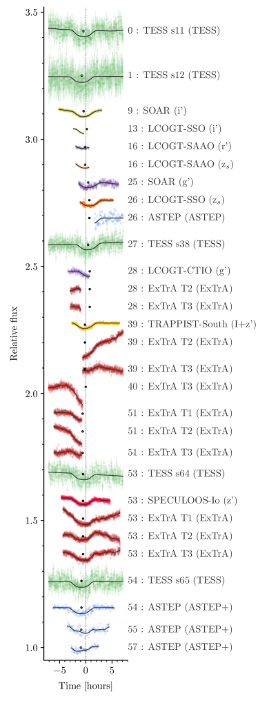
Figure 1: Transit observations (vertical error bars) with the model that combines both transit and noise (median as a black line and 68% interval in gray), arbitrarily shifted vertically. Each transit observation is labeled with the transit epoch, the telescope, and the observing band. Each transit is centered relative to the maximum a posteriori value of the linear ephemeris derived in Sect. 4.1. Horizontal error bars show the mid-transit time offset from the linear ephemeris.

2.2 ExTrA

The ExTrA (Bonfils et al. 2015) is a low-resolution near-infrared (0.85 to 1.55 $\mu$m) multi-object spectrograph fed by three 60-cm telescopes located at La Silla Observatory in Chile. One full and four partial transits were observed using one, two, or three of the ExTrA telescopes. We used 8$\arcsec$ aperture fibers and the lowest-resolution mode ($R$$\sim$20) of the spectrograph, a combination that is optimal for the target’s magnitude, with an exposure time of 60 seconds. Five fibers are positioned in the focal plane of each telescope to select light from the target and four comparison stars. We chose comparison stars with 2MASS $J$ magnitudes (Skrutskie et al. 2006) and effective temperatures (Gaia Collaboration et al. 2018) similar to the target. The resulting ExTrA data were analyzed using custom data reduction software.

2.3 SPECULOOS

The SPECULOOS Southern Observatory is located at ESO Paranal Observatory in Chile (Jehin et al. 2018; Delrez et al. 2018; Sebastian et al. 2021). It holds four Ritchey-Chrétien 1m-class telescopes, each equipped with a deep-depletion Andor $2048\times 2048$ CCD camera with a pixel scale of $0.35\arcsec$, which gives a field of view of $12\times 12\arcmin$. We observed one full transit of TOI-1227 b in the Sloan-z’ filter on the night of 3 May 2023 with an exposure of 21 seconds, totaling 1033 measurements. The data reduction and photometry extraction were performed with a custom pipeline built with the prose package (Garcia et al. 2022).

2.4 TESS

In addition to the sectors 11, 12, and 38 TESS data presented in Mann et al. (2022), TESS observed two full transits of TOI-1227 b in sectors 64 and 65 with 2-min cadence. For the analysis in Sect. 3, we used the presearch data conditioning simple aperture photometry (PDCSAP; Smith et al. 2012, Stumpe et al. 2012, 2014, Caldwell et al. 2020) light curve of TOI-1227, produced by the TESS Science Processing Operations Center (SPOC; Jenkins et al. 2016; Caldwell et al. 2020).

2.5 TRAPPIST

The TRAPPIST-South is a 0.6-m Ritchey-Chrétien telescope located at ESO La Silla Observatory in Chile (Jehin et al. 2011; Gillon et al. 2011). It is equipped with a German equatorial mount and has a $2048\times 2048$ back-illuminated FLI ProLine PL3041-BB CCD camera with a pixel scale of $0.64\arcsec$, giving a field of view of $22\times 22\arcmin$. One full transit of TOI-1227 b was observed on 15 April 2022 with an exposure time of 180 seconds in the I+z custom filter, and we collected 170 measurements during the observation. We performed the data analysis using a custom pipeline built with the prose package, which allowed for the data to be reduced as well as for differential photometry to be performed.

In the transit light curves presented in this work, no detrending was applied for systematics. Any systematics present in the light curves were addressed during the global analysis (Sect. 3).

3 Transit photometry analysis

We derived the transit times of TOI-1227 b with juliet (Espinoza et al. 2019), using batman (Kreidberg 2015) for the transit model, and the approximate Matern kernel Gaussian process (GP) included in celerite (Foreman-Mackey et al. 2017) to model the systematics. We used different GPs’ hyperparameters for each telescope and for each transit observation. The timing of each transit epoch, observed with one to five telescopes, is a free parameter. We assumed a circular orbit, but this assumption should not significantly affect the determination of the transit times. We adopted non-informative or broad priors for all the parameters. To sample from the posterior, we used the dynesty nested sampling code (Speagle 2020). The complete list of parameters, priors, and posteriors’ median and 68.3% credible interval (CI) are shown in Table 2. We scaled the radius of TOI-1227 b using the Mann et al. (2022) stellar radius, $0.56\pm 0.03$ $R_{\odot}$. Figure 1 shows the data and the model posterior. We explain how we briefly tested the accuracy of our transit timings using simulated transits in Sect. B.

Table 2: Inferred parameters from the transit photometry analysis.

Parameter	Units	Prior	Posterior median and 68.3% CI
TOI-1227
Mean density, $\rho_{\star}$	[$\mathrm{g\;cm^{-3}}$]	$U(0.9,1.6)$	$1.197\pm 0.063$
$q_{1}$ ASTEP, ExTrA, TESS		$U(0,1)$	$0.18^{+0.18}_{-0.12}$, $0.19^{+0.22}_{-0.13}$, $0.25^{+0.31}_{-0.17}$
$q_{2}$ ASTEP, ExTrA, TESS		$U(0,1)$	$0.62^{+0.27}_{-0.36}$, $0.33^{+0.37}_{-0.24}$, $0.32^{+0.37}_{-0.23}$
$q_{1}$ g’, r’, i’		$U(0,1)$	$0.70^{+0.20}_{-0.26}$, $0.50\pm 0.34$, $0.77^{+0.15}_{-0.20}$
$q_{2}$ g’, r’, i’		$U(0,1)$	$0.71^{+0.20}_{-0.32}$, $0.63^{+0.27}_{-0.39}$, $0.64^{+0.21}_{-0.24}$
$q_{1}$ z’, zS, I+z		$U(0,1)$	$0.71^{+0.19}_{-0.22}$, $0.61\pm 0.24$, $0.883^{+0.086}_{-0.16}$
$q_{2}$ z’, zS, I+z		$U(0,1)$	$0.26^{+0.24}_{-0.17}$, $0.43^{+0.29}_{-0.25}$, $0.46\pm 0.21$
TOI-1227 b
Semi-major axis, $a$	[au]		$0.0942\pm 0.0053$
Inclination, $i_{p}$	[°]		$88.711\pm 0.036$
Radius ratio, $R_{\mathrm{p}}/R_{\star}$			$0.1567\pm 0.0029$
Scaled semi-major axis, $a/R_{\star}$			$36.18\pm 0.62$
Impact parameter, $b$			$0.814\pm 0.012$
Transit duration, $T_{14}$	[h]		$4.752^{+0.052}_{-0.074}$
Radius, $R_{\mathrm{p}}$	[$\mathcal{R}^{\rm N}_{e\rm E}$]		$9.58\pm 0.55$
	[$\mathcal{R}^{\rm N}_{e\rm J}$]		$0.854\pm 0.049$
$r_{1}$		$U(0,1)$	$0.8759^{+0.0071}_{-0.0080}$
$r_{2}$		$U(0.140,0.175)$	$0.1567\pm 0.0029$
Mid-transit times
Epoch 0 (TESS s11)	[BJDTDB]	$U(2458617.44,2458617.53)$	$2458617.4817\pm 0.0081$
Epoch 1 (TESS s12)	[BJDTDB]	$U(2458644.76,2458644.90)$	$2458644.830\pm 0.015$
Epoch 9 (SOAR i’)	[BJDTDB]	$U(2458863.71,2458863.76)$	$2458863.7372\pm 0.0028$
Epoch 13 (LCOGT i’)	[BJDTDB]	$U(2458973.17,2458973.25)$	$2458973.2089\pm 0.0048$
Epoch 16 (LCOGT r’, zS)	[BJDTDB]	$U(2459055.230,2459055.309)$	$2459055.2799^{+0.0036}_{-0.012}$
Epoch 25 (SOAR g’)	[BJDTDB]	$U(2459301.48,2459301.65)$	$2459301.5581^{+0.0062}_{-0.0052}$
Epoch 26 (ASTEP, LCOGT zS)	[BJDTDB]	$U(2459328.915,2459328.945)$	$2459328.9290\pm 0.0015$
Epoch 27 (TESS s38)	[BJDTDB]	$U(2459356.24,2459356.32)$	$2459356.2810\pm 0.0063$
Epoch 28 (LCOGT g’, ExTrA T23)	[BJDTDB]	$U(2459383.60,2459383.70)$	$2459383.6550\pm 0.0041$
Epoch 39 (ExTrA T23, TRAPPIST-South I+z)	[BJDTDB]	$U(2459684.58,2459684.615)$	$2459684.5931^{+0.0018}_{-0.0014}$
Epoch 40 (ExTrA T3)	[BJDTDB]	$U(2459711.900,2459712.005)$	$2459711.9615^{+0.0078}_{-0.010}$
Epoch 51 (ExTrA T123)	[BJDTDB]	$U(2460012.890,2460012.935)$	$2460012.9133\pm 0.0029$
Epoch 53 (ExTrA T123, SPECULOOS z’, TESS s64)	[BJDTDB]	$U(2460067.63,2460067.65)$	$2460067.6395\pm 0.0012$
Epoch 54 (ASTEP, TESS s65)	[BJDTDB]	$U(2460094.97,2460095.01)$	$2460094.9886\pm 0.0031$
Epoch 55 (ASTEP)	[BJDTDB]	$U(2460122.30,2460122.40)$	$2460122.3472^{+0.015}_{-0.0093}$
Epoch 57 (ASTEP)	[BJDTDB]	$U(2460177.02,2460177.12)$	$2460177.0688^{+0.0077}_{-0.0068}$
Photometry
Offset relative flux	[Relative flux]	$N(0,0.01)$	(a)
Jitter	[ppm]	$J(1,20000)$	(a)
Amplitude of the GP	[Relative flux]	$J(10^{-6},1.0)$	(a)
Timescale of the GP	[days]	$J(0.001,10)$	(a)

For comparison, we repeated the analysis for a model with equally spaced transits. This required using a linear ephemeris for the timing of each transit epoch ($E$), calculated as $T_{0}+P\times E$, where $T_{0}$ is the transit time at a reference epoch and $P$ is the orbital period and both are free parameters. A Bayesian model comparison strongly favors (Kass & Raftery 1995) the model with TTVs over the linear ephemeris model, by a log-Bayes factor $\mathcal{Z}_{\rm TTVs}/\mathcal{Z}_{T_{0},P}$ of $54.5\pm 0.6$. This finding brings novel evidence that the transits of TOI-1227 A are indeed produced by a planet, as eclipse-timing variations of the observed amplitude would imply a stellar mass perturber (Rappaport et al. 2013). Such a perturber would have been observed in the spectra or the color-magnitude diagram (Mann et al. 2022). The alternative false positive scenarios involving starspots or an accretion disk, presented in Yu et al. (2015) for the young system PTFO 8-8695, do not apply here. This is because the orbital period (27.4 days) is significantly different from the rotation period of the star (1.65 days) and TOI-1227 shows no evidence of having an accretion disk.

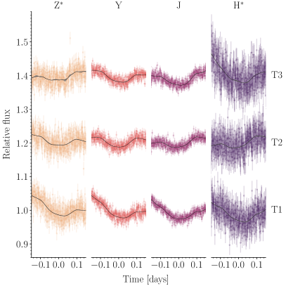
Figure 7: ExTrA full transit photometry observation of TOI-1227 b in Z*, Y, J, and H* bands (error bars). Each line corresponds to an ExTrA telescope (labeled T1, T2, and T3) observation that is offset vertically for clarity. For each transit the median model (black line) and 68% CI (gray band, barely visible) computed from 1000 random posterior samples are shown.

We extended the transit chromatic analysis of Mann et al. (2022) by including the additional photometric bands made available by our new observations. We excluded the epoch 16 transit (LCOGT-SAAO r’, z_S) which lacks a baseline and the partial transits observed by ExTrA. We separated the five TESS sectors because they use distinct photometric aperture and could therefore have different third light contamination. To refine the chromatic analysis, we synthesized photometry in the UKIRT-WFCAM filters from the ExTrA spectrophotometry for the fully observed epoch 53 transit. This produced four intermediate-band light curves in addition to the light curve in ExTrA’s full wavelength range (0.85 to 1.55 $\mu$m), for a truncated Z band (Z^∗), a Y, a J, and a truncated H band (H^∗) (Fig. 7). This chromatic analysis is similar to the one presented above, except that the planet-to-star radius ratio ($R_{p}/R_{\star}$) has been adjusted separately for each dataset. This allowed for a different transit depth at each band, whose posteriors are listed in Table 5. As Fig. 2 shows, the transit depths for all of these bandpasses are consistent with a common $R_{p}/R_{\star}$. The observed achromaticity of the transit reinforces the hypothesis of a planet rather than a blended binary scenario.

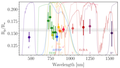
Figure 2: Posterior distribution comparison for $R_{p}/R_{\star}$ (error bars) computed for different bands (whose transmission curves are shown and labeled with different colors) and TESS sectors (shifted horizontally for visualization purposes, the TESS sector number is noted inside the dots). All transits were fitted jointly with a separate $R_{p}/R_{\star}$ parameter for each band. The horizontal solid and dotted gray lines represent the posterior median and 68.3% CI assuming a common $R_{p}/R_{\star}$ (Sect. 3).

4 Modeling the transit timings

Although the TTVs are robustly detected, their modeling is challenging because the transit observations are heterogeneous and they do not cover the full range of the timing variability yet. Additionally, half of the epochs have only partial transit coverage, providing timings that are less robust than from a full transit observation.

4.1 Sine wave model

We started modeling the transit timings assuming a transit period that oscillates sinusoidally around an average value, which is often a good approximation for planets near first-order resonance (Lithwick et al. 2012) and inside resonance (Nesvorný & Vokrouhlický 2016). We excluded from the analysis transit epoch 16, which covers neither the first nor the fourth contact. The posterior distribution was sampled using the emcee algorithm (Goodman & Weare 2010; Foreman-Mackey et al. 2013). We used uniform priors for all parameters. The posteriors are listed in Table 3, and Fig. 3 shows the observed TTVs with the sinusoidal model posterior. The maximum a posteriori (MAP) linear ephemeris, which was used to compute the TTVs in Figs. 1, 3, 6, and 8, is BJD_TDB 2460067.6617 + 27.36152 $\times$ $E$, with $E$ being the epoch number relative to epoch 53. This simple model does not fit epochs 54 and 57 well, and the main periodicity of the TTVs is probably longer than the 3.7 year-long sine wave period. There are tentative indications of ”chopping” (Deck & Agol 2015), for example the ”jump” between transit epochs 53 and 54, but more transit observations are clearly needed to characterize the TTVs.

Table 3: Sine wave modeling of the TTVs.

Parameter	Units	Median and 68.3% CI
$T_{0}$	[BJDTDB]	$2460067.6622\pm 0.0027$
Orbital period, $P$	[days]	$27.36155\pm 0.00015$
Sine $t_{s}$	[epochs]	$-15.62\pm 0.38$
Sine period, $P_{s}$	[epochs]	$49.3\pm 2.7$
Sine amplitude, $A$	[minutes]	$40.1\pm 2.8$

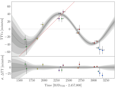
Figure 3: Posterior TTVs of TOI-1227 b computed relative to a linear ephemeris (from the MAP value of the sinusoidal model) are shown with black error bars (Sect. 3). In the upper panel, the TTVs’ sinusoidal model (median, 1, 2, and 3-$\sigma$, in gray) is shown and compared with individual transit-time determinations (Sect. 3, median and 68% CI, the colors of the dots indicate the observing band as in Fig. 1). The linear ephemeris from Mann et al. (2022) is shown as a red line. In the lower panel, the posterior median of the TTVs’ model was subtracted to visualize the uncertainty of the distribution and to allow for better comparison with the individual transit-time determinations.

4.2 Nonparametric model

Although a sinusoidal model may be an adequate model, it risks lacking the flexibility to capture the intricacies produced by the actual planetary dynamics. On the other hand, N-body simulations are costly and often quite slow. In any case, a model correctly accounting for TTVs is needed to correctly estimate the planetary ephemeris.

For this subsection, we used a nonparametric model for the TTVs. More concretely, the variations with respect to a constant linear ephemeris were modeled using GP regression (Rasmussen & Williams 2005; Rajpaul et al. 2015). The covariance of the model is given by a kernel function, whose hyperparameters were optimized simultaneously to the determination of the ephemeris parameters, $P$ and $T_{0}$.

Several kernel functions were tried. Leveraging the fact that the sum and product of two valid kernel functions is also a valid kernel function, we constructed a series of models based on the following:

1. the squared exponential function – the radial basis function (RBF),

   $$k(t_{i},t_{j})=A^{2}\exp\left(-\frac{d(t_{i},t_{j})^{2}}{2\tau^{2}}\right)\;\;,$$ (1)

   where $A^{2}$ is the covariance amplitude, the variable $t_{i}$ is the epoch of $i$-th transit epoch, and $d$ is a function computing the distance, here $d(t_{i},t_{j})=t_{i}-t_{j}$;

2. the exp-sine function (i.e., a strictly periodic kernel),

   $$k(t_{i},t_{j})=A^{2}\exp\left(-\frac{2\sin^{2}(\pi\,d(t_{i},t_{j})/\mathcal{P})}{\epsilon^{2}}\right)\;\;,$$ (2)

   where $\mathcal{P}$ is the covariance periodicity; and

3. a quasi-periodic function (i.e., the product of the squared exponential and the exp-sine kernels).

In addition, we explored the inclusion of a white noise term in the covariance (i.e., a diagonal kernel function). Readers can refer to Rasmussen & Williams (2005) for a description of each kernel function.

Vague priors were set for the parameters of the linear mean model, $P$ and $T_{0}$, by using a normal prior with large variance. In this manner, the marginal likelihood of the model can be computed analytically. The marginal likelihood thus computed was optimized with respect to the hyperparameters using the limited-memory Broyden–Fletcher–Goldfarb–Shanno (LM-BFGS) algorithm implemented in the Python scipy package optimize (Jones et al. 2001).

Overall, we found that kernels without a periodic term (the RBF kernel) produced worse results than those with a periodic term. Also, quasi-periodic kernels have very long decay times, in agreement with the fact that – at most – a single period is covered by the current observations. In fact, the periodic and quasi-periodic solutions were identical in all aspects, and are therefore not reported.

If the kernel functions enumerated above are combined with a long-term trend modeled by summing an additional RBF function,

$$A_{\text{long}}\exp\left(-\frac{d(t_{i},t_{j})^{2}}{\tau_{\text{long}}^{2}}\right)\;\;,$$ (3)

the values of the marginal likelihood are maximized, but the error in the mean orbital period is increased significantly. These solutions, though favored by the data, imply that the currently observed transits are only covering a small fraction of the much longer evolution with timescale $\tau_{\text{long}}$ of about 185 transit epochs, that is, over 13 years.

The results of all the tested kernel functions are listed in order of increasing optimized marginal likelihood in Table 4. The value of the selected parameters are presented. We remind the reader that the values of the hyperparameters are optimized, and that they should therefore be considered with caution. On the other hand, for the period and the epoch of the transits of TOI-1227 b, we have full Gaussian posterior distributions, whose summaries are provided. However, these distributions are conditional on the values of the hyperparameters.

We note that the solutions from kernels including a white noise component (+ white) imply an additional white noise term with an amplitude between 6.4 and 8.3 minutes. This may seem excessive in view of the current data, but our objective for this work was to avoid constraining the model drastically by setting bounds on the optimization. We also present the alternative models without a diagonal term added to the model covariance. In all cases, the uncertainty of the period and epoch of transits increased significantly with respect to the values in Table 3, because this approach adequately propagates the uncertainty of the TTV model into the ephemeris. In Fig. 4 we present the best model (per + long + white), the best model without a long-term trend (per + white), and the best model with neither a long-term trend nor white noise component (per).

Table 4: Results of the GP regression model to the transit times.

kernel	period, $P$	$\sigma_{P}$	$T_{0}$	$\sigma_{T_{0}}$	cov. amplitude, $A$	cov. periodicity, $\mathcal{P}$	$\sigma_{\text{white}}$	logL
	[d]	[d]	[BJD${}_{\text{TDB}}$ - 2,460,000]		[min]	[epochs]	[min]
RBF	27.36090	0.00070	67.636	0.023	41.63	–	–	23.25
per	27.36109	0.00014	67.648	0.010	29.85	48.02	–	25.52
RBF + white	27.36108	0.00086	67.637	0.030	48.69	–	8.3	28.55
per + white	27.36130	0.00025	67.651	0.043	67.77	61.47	8.0	28.68
per + long	27.36172	0.01256	66.218	1.968	12.38	29.92	–	29.01
per + long + white	27.36207	0.01324	66.102	2.131	15.40	29.56	6.4	29.46

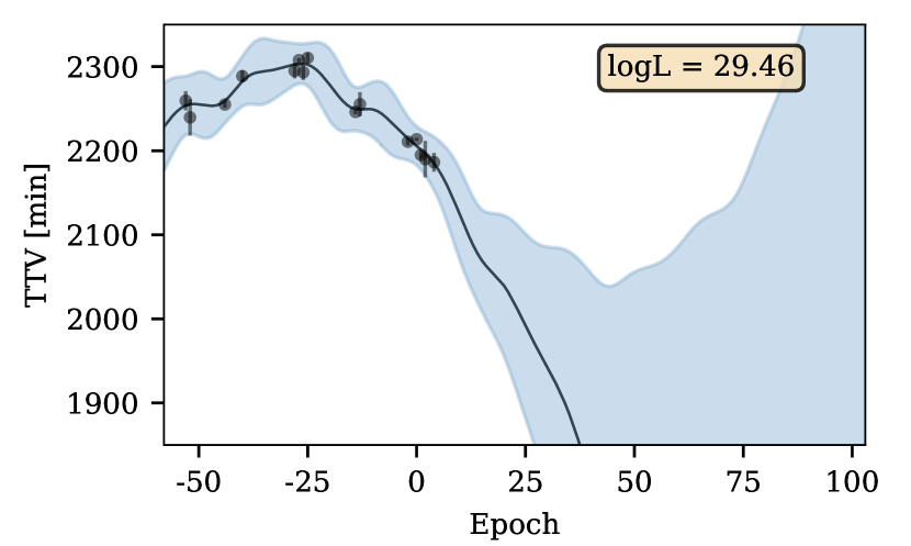
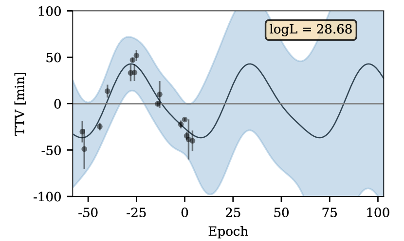
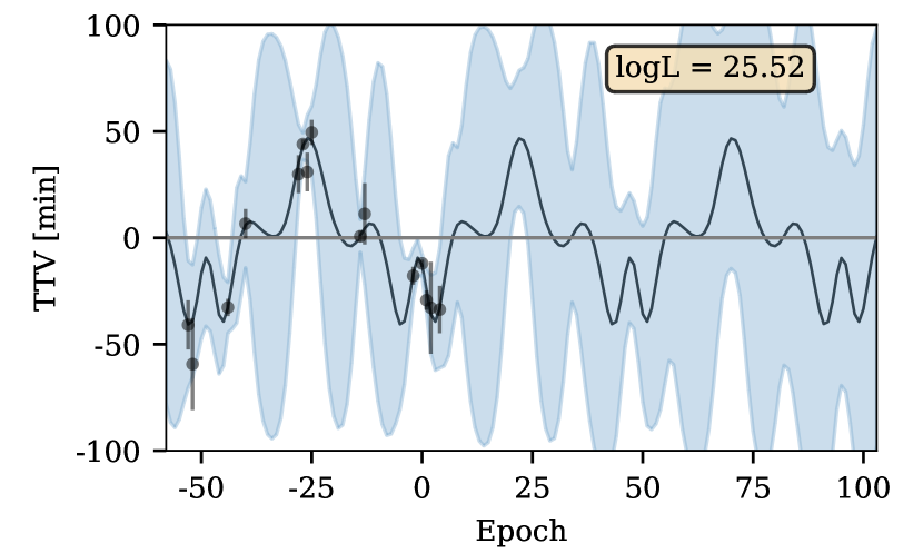
Figure 4: GP regression of the time variations in excess of mean linear ephemeris. The results are shown for kernels ”per + long + white” (top), ”per + white” (middle), and ”per” (bottom). The black curve represents the posterior GP mean and the blue-shaded area represents the 3-$\sigma$ region for each epoch. The epoch number is relative to epoch 53.

4.3 Dynamical modeling

We have attempted to develop a physical model of the TTVs, exploring inner and outer perturbers around the first and second order mean motion resonances (exploring period ratios from 3:1 to 6:5). We assumed coplanar orbits and neglected the light-time effect (Irwin 1952), which is very small at these periods. We used the REBOUND n-body code (Rein & Liu 2012) with the WHFast integrator (Rein & Spiegel 2015) and an integration step of 0.01 days. We did not impose a stability criterion. The model was parameterized using, for each planet, the planet-to-star mass ratio, a pseudo-period, the time of a reference conjunction (star, planet, and observer), and two products of the square root of the eccentricity: one multiplied by the cosine of the argument of periastron, and another multiplied by the sine of the argument of periastron. We used uniform priors for all parameters. The joint posterior distribution was sampled using the emcee algorithm. We started the walkers for a 10 $\mathrm{M_{E}}$ mass for TOI-1227 b, a plausible value following Mann et al. (2022), and a perturber offset from the period commensurability in accordance with a TTVs’ super-period (Lithwick et al. 2012) of 3.7 years.

While we have not explored the entire parameter space of these orbital configurations, we have already found multiple very distinct solutions that provide a satisfactory fit. Figure 5 shows the posterior for the perturber and TOI-1227 b masses and a metric for the goodness of fit ($\chi^{2}_{\rm red}$). The best fit was obtained for an exterior 3:2 MMR. In this case, the TOI-1227 b mass distribution is bimodal, with a peak at $40\ \mathrm{M}_{\oplus}$ and a perturber of mass $5.7\pm 1.7\ \mathrm{M}_{\oplus}$. The next best fits correspond to the inner resonances 5:7, 7:9, and 4:5. However, these fits show an indication of overfitting, with very small masses for the perturber and very constrained mass ranges for TOI-1227 b. These configurations could be ruled out with a longer TTV coverage, resolving the super-period.

The MAP model for each period ratio tested is plotted in Fig. 6. Even with the simplistic assumption of coplanar orbits, the dynamical model is flexible enough to capture the observed TTVs, including the jump between epochs 53 and 54. This exercise proves that the TTVs can be reasonably fitted with several orbital configurations, and thus that the problem is degenerate with the current dataset. We again conclude that more data are needed to find the right solution. The problem naturally becomes more complex if additional dynamically relevant perturbers are present in the system.

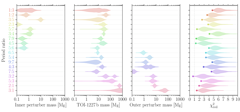
Figure 5: Exploration of perturbers near the inner and outer first and second order resonances (the period ratio is denoted in the format ”perturber:TOI-1227 b”). From left to right: Violin plots representing the marginal posterior of the mass for the inner perturber, the mass of TOI-1227 b, the mass of the outer perturber, and the goodness of fit ($\chi^{2}_{\rm red}$), with the MAP value displayed as a dot.

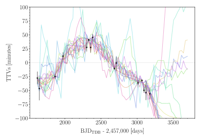
Figure 6: Same as the upper panel of Fig. 3 but showing the MAP models of the exploration of the perturbers close to the inner and outer first and second order resonances. The color code is the same as in Fig. 5.

5 Results and discussion

We have detected significant TTVs of the 11 Myr exoplanet TOI-1227 b. Those TTVs are well above what could be explained by spots (TOI-1227 shows rotational modulation in the TESS light curve with a period of 1.65 days): they amount to 14% of the transit duration (see Fig. 8), while spots can cause TTVs of $\sim$1% of the transit duration at most (Ioannidis et al. 2016). We conclude that the observed TTVs are most likely caused by at least one additional planet in the system, but additional transit observations are needed to constrain the orbital configuration.

One probable perturber could be the external 3:2, with a mass of $5.7\pm 1.7$ $\mathrm{M_{E}}$. Among the configurations tested, the external 3:2 perturber provided the best fit to the data. Interestingly, capture into the 3:2 is the typical expected outcome of convergent type I migration for sub-Neptunes (Kajtazi et al. 2023). In addition, the configuration is stable during the migration phase as the outer perturber is less massive than the inner one (Deck & Batygin 2015). Unfortunately, if this perturber is coplanar with TOI-1227 b, it will not transit.

In addition to detecting TTVs, the additional transit observations slightly improve the transit parameters derived in Mann et al. (2022). Specifically, grazing transits are now ruled out, eliminating the tail of high planet-to-star radius ratios in the posterior. The planetary radius we derived in ($0.854\pm 0.049$ $\mathrm{R}_{\rm J}$) precisely matches the one of Mann et al. (2022), $0.854^{+0.067}_{-0.052}$ $\mathrm{R}_{\rm J}$, with just slightly improved error bars. While the planet-to-star radius ratio now has a 1.9% uncertainty, the planetary radius is uncertain by 5.7%, dominated by the 5.4% uncertainty on the stellar radius. The planet-to-star radius ratio measurement may also be biased, as it assumes an unspotted star (Czesla et al. 2009).

We expanded the transit chromatic analysis of Mann et al. (2022), and again found no significant chromaticity. It is anticipated that depths will increase at optical wavelengths due to the presence of unocculted spots. However, the g’ measurement suggests that spots may not significantly influence the measurement of the planet-to-star radius ratio. An alternative interpretation could be that the spots are distributed semi-uniformly. This implies that there is roughly an equal number of unocculted and occulted spots and, as a result, their effects would largely neutralize each other.

Based on our understanding, there are no false positive scenarios that could account for the observed 40-minute TTVs of TOI-1227 b. As a result, these observations appear to unequivocally confirm TOI-1227 b as a planet. We encourage intensive observations of TOI-1227 b’s transits, as they could lead to a measurement of the planet’s mass.

TOI-1227 b provides a rare opportunity for transmission spectroscopy of a still-contracting young exoplanet using JWST (Gardner et al. 2006) or high-resolution spectrographs, although starspots may pose a challenge (Rackham et al. 2018). The transmission spectroscopy metric (TSM, Kempton et al. 2018) could range from 95 to 950 for a mass of 50 and 5 $\mathrm{M_{E}}$, respectively. However, before attempting this observation, we should improve the forecast of TOI-1227 b transits. Additionally, measuring the mass of TOI-1227 b would aid in better interpreting the transmission spectrum.

Appendix A Additional figures and tables

Table 5: Inferred $R_{p}/R_{\star}$ in different bands and TESS sectors.

Band	$\lambda_{\rm pivot}$ [nm]	Prior	Median and 68.3% CI
g’	476	$U(0,1)$	$0.142\pm 0.011$
TESS s11	770	$U(0,1)$	$0.176\pm 0.018$
TESS s12	770	$U(0,1)$	$0.184\pm 0.024$
TESS s38	770	$U(0,1)$	$0.161\pm 0.014$
TESS s64	770	$U(0,1)$	$0.152\pm 0.015$
TESS s65	770	$U(0,1)$	$0.152\pm 0.013$
i’	772	$U(0,1)$	$0.1463\pm 0.0087$
ASTEP+ Red	819	$U(0,1)$	$0.1430\pm 0.0093$
I+z	850	$U(0,1)$	$0.1628\pm 0.0075$
zS	867	$U(0,1)$	$0.1549_{-0.0048}^{+0.0056}$
ExTrA $Z^{*}$	890	$U(0,1)$	$0.154\pm 0.015$
z’	$\sim$912	$U(0,1)$	$0.1581\pm 0.0062$
ExTrA $Y$	1031	$U(0,1)$	$0.160\pm 0.011$
ExTrA	1165	$U(0,1)$	$0.163\pm 0.017$
ExTrA $J$	1248	$U(0,1)$	$0.165\pm 0.016$
ExTrA $H{*}$	1526	$U(0,1)$	$0.151_{-0.028}^{+0.025}$

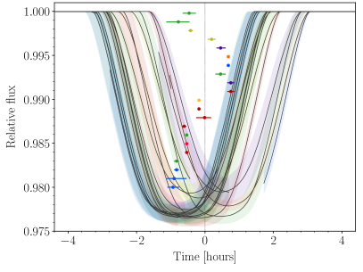
Figure 8: Posterior of the transit models for each epoch and band (Sect. 3, TTV analysis with a single $R_{p}/R_{\star}$), with the median represented as a black line and the 68% credible interval shown in various colors corresponding to Fig. 1, excludes epoch 16. Each transit is centered relative to the MAP value of the linear ephemeris derived in Sect. 4.1. The horizontal error bars indicate the mid-transit time offset from the linear ephemeris, shifted vertically, with time increasing from top to bottom.

Appendix B Supplementary assessment

In order to validate the accuracy of our methodology in determining transit times, we applied the methods outlined in Sect. 3 to simulated data. We started from the true observation, removed the MAP model from the analysis presented Sect. 3, and then added back the same model but with a different mid-transit time. The simulated times were pure linear ephemeris (no TTVs) for simulation 1, and the MAP sinusoidal model of Sect. 4.1 for simulation 2. This procedure tests the original data (with its systematics and sampling) at slightly different times. We have excluded epoch 16, which was not used for Sect. 4. Figure 9 compares posterior and simulated transit times. To further compare the posteriors with the simulated values, we calculated the offset normalized by the 68.3% CI. This metric has a mean of 0.11 and 0.20, and a standard deviation of 0.88 and 0.86, for simulations 1 and 2, respectively. This is compatible with a standard normal distribution, given the small number of samples, suggesting that the systematics do not prevent an accurate estimation of the transit timing.

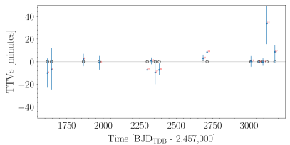
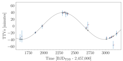
Figure 9: Posterior TTVs of the simulated data (simulation 1 in the upper panel and simulation 2 in the lower panel), relative to a linear ephemeris, are shown with blue error bars. The open black circles are the simulated data, and the gray line is the simulated model for the TTVs.