Universal hard-edge statistics of non-Hermitian random matrices

Abstract

Random matrix theory is a powerful tool for understanding spectral correlations inherent in quantum chaotic systems. Despite diverse applications of non-Hermitian random matrix theory, the role of symmetry remains to be fully established. Here, we comprehensively investigate the impact of symmetry on the level statistics around the spectral origin—hard-edge statistics—and complete the classification of spectral statistics in all the 38 symmetry classes of non-Hermitian random matrices. Within this classification, we discern 28 symmetry classes characterized by distinct hard-edge statistics from the level statistics in the bulk of spectra, which are further categorized into two groups, namely the Altland-Zirnbauer₀ classification and beyond. We introduce and elucidate quantitative measures capturing the universal hard-edge statistics for all the symmetry classes. Furthermore, through extensive numerical calculations, we study various open quantum systems in different symmetry classes, including quadratic and many-body Lindbladians, as well as non-Hermitian Hamiltonians. We show that these systems manifest the same hard-edge statistics as random matrices and that their ensemble-average spectral distributions around the origin exhibit emergent symmetry conforming to the random-matrix behavior. Our results establish a comprehensive understanding of non-Hermitian random matrix theory and are useful in detecting quantum chaos or its absence in open quantum systems.

I Introduction

Symmetry plays a pivotal role in random matrix theory and is crucial for comprehending spectra of complex systems [1]. Dyson’s threefold way initially classifies Hermitian random matrices according to time-reversal symmetry (TRS) [2]. The bulk of spectra is characterized by the threefold universal level statistics, termed the Wigner-Dyson statistics [3, 4]. These universal level statistics appear in the following renowned random matrix ensembles: Gaussian unitary ensemble (lacking TRS), Gaussian orthogonal ensemble (possessing TRS with sign $+1$), and Gaussian symplectic ensemble (possessing TRS with sign $-1$). Extensive theoretical and experimental investigations have demonstrated that the spectral correlations of chaotic closed quantum systems align with these universal random-matrix statistics with corresponding symmetry [5, 6, 7, 8, 9]. Subsequently, random matrix ensembles in the chiral and Bogoliubov-de Gennes (BdG) symmetry classes, which incorporate chiral symmetry [10, 11] and particle-hole symmetry [12], were introduced. These symmetries dictate universal properties in the proximity of the symmetry-preserving point $E=0$ in the energy spectrum. Together with TRS, chiral and particle-hole symmetries form the comprehensive classification of Hermitian random matrices, known as the Altland-Zirnbauer (AZ) tenfold classification [12]. Importantly, this well-established Hermitian random matrix theory has found broad applications across diverse fields of physics. In condensed matter physics, it elucidates universal transport phenomena of disordered metals and superconductors [13, 14] and also serves as a powerful tool to detect the Anderson transitions [15] and many-body-localization transitions [16, 17]. In nuclear physics, random matrices provide an effective model of chiral symmetry breaking [18].

While researchers historically focused on Hermitian operators, non-Hermitian operators are equally important in various physical systems. Prime examples include chiral Dirac operators with chemical potential in quantum chromodynamics (QCD) [19, 20, 21] and scattering matrices in quantum transport phenomena [13, 14]. Non-Hermitian matrices appear naturally in stochastic processes and network systems, having important applications in biological systems  [22, 23, 24, 25, 26, 27, 28, 29]. Realistic physical systems are inevitably coupled with their surrounding environments, and non-Hermitian operators also play pivotal roles in the dynamics of such open physical systems [30]. For the Markovian environment, the dynamics of open quantum systems is described by the Lindblad master equation [31, 32], where the generator of the dynamics, known as the Lindbladian, is a non-Hermitian operator. The time evolution of classical synthetic materials such as optical and photonic systems with energy gain or loss [33, 34, 35, 36], along with quantum systems under continuous measurement [37, 38, 39, 40], can also be characterized by non-Hermitian Hamiltonians. Thanks to advances in state-of-the-art experiments and theories, the past years have witnessed remarkable development in non-Hermitian physics [41, 42, 43, 44].

These advances necessitate a systematic understanding of symmetry inherent in open quantum systems, leading to the 38-fold classification [45, 46] of non-Hermitian operators beyond the tenfold classification of Hermitian operators. This symmetry classification serves as a guiding principle in designing and comprehending non-Hermitian topological phases [47, 48, 49, 50, 51, 46, 52], analyzing non-Hermitian Anderson [53, 54, 55, 56, 57, 58, 59, 60, 61, 62, 63, 64, 65, 66] and many-body localization [67, 68, 69], as well as understanding spontaneous breaking of parity-time ($\mathcal{PT}$) symmetry [70]. Moreover, the chaotic behavior in open quantum systems has drawn substantial attention [71, 72, 73, 74, 75, 76, 77, 78, 79, 80, 81, 82, 83, 84, 85], with symmetry playing a crucial role in its description. Researchers developed the symmetry classification of non-Hermitian generalizations of the Sachdev-Ye-Kitaev (SYK) model [86, 87, 88, 89, 90, 91, 92], a prototype of quantum chaotic model, revealing rich structures [93]. Substantial progress was also made in the symmetry classification of Lindbladians for both single-particle and many-body systems [94, 95, 96, 97]. Several prototypical models, such as Bogoliubov quasi-particles in dissipative superconductors [98, 99, 100, 101, 102] and non-Hermitian extensions [103, 104, 49] of the Su-Schrieffer-Heeger model [105], exhibit particle-hole or sublattice symmetry and can display chaotic behavior in the presence of disorder.

Non-Hermitian random matrix theory is useful for understanding the spectral correlations and dynamics of open quantum systems. It was conjectured that the statistics of complex energy levels in non-integrable open quantum systems follow those of non-Hermitian random matrices, which has been numerically verified in several models [71, 77, 78, 79, 82]. Level correlations of non-Hermitian random matrices in the bulk of complex spectra (i.e., away from special points, lines, and edges of complex spectra) belong to the threefold universality classes [106, 72, 77]. These universality classes depend only on an extension of TRS for non-Hermitian operators, time-reversal symmetry^† [46], while the influence of other defining symmetries appears elusive. Given the prevalence of almost all 38 symmetry classes in realistic physical systems (e.g., see Refs. [93, 96, 97]), characterizing the unique universality classes of level correlations in each symmetry class and exploring the impact of symmetry stands out as one of the crucial challenges in non-Hermitian random matrix theory. Despite its importance and some discrete works on level statistics beyond the threefold way, especially those on non-Hermitian but real random matrices [107, 108, 109, 110, 111], a comprehensive understanding of the universality classes within the 38-fold symmetry classification is still lacking.

In this work, we demonstrate that the level statistics around the spectral origin, known as the hard-edge statistics, faithfully reveal the impact of all defining symmetries. We comprehensively explore possible universality classes of the hard-edge statistics of non-Hermitian random matrices in all 38 symmetry classes. We identify 28 symmetry classes where the level statistics around the spectral origin differ from those in the bulk of the spectra or around the real or imaginary axis by analyzing their defining symmetry. This approach is akin to that in Hermitian random matrix theory, where the hard-edge statistics distinct from the bulk statistics appear in the chiral and BdG symmetry classes but not in the Wigner-Dyson symmetry classes [12, 14, 1]. By contrast, non-Hermiticity enriches the symmetry classification and leads to more diverse universal spectral correlations. Specifically, we categorize these 28 symmetry classes into two groups and investigate all of them, summarized in Table 2 and Table 3.

The first group, summarized in Table 2, comprises seven symmetry classes, where the spectral origin is the only high-symmetry point in the complex plane, and the hard-edge statistics exhibit spectral U(1) rotation symmetry. These seven symmetry classes, together with the threefold classes based on time-reversal symmetry^†, form the tenfold classification, which we dub Altland-Zirnbauer₀ (AZ₀) classification. We employ the density of complex eigenvalues and the distributions of the complex level ratios around the spectral origin to characterize the universality classes of the hard-edge statistics. We numerically obtain seven universal ratio distributions and summarize their properties in Table 2. We explain their asymptotic behaviors through analytic small-matrix calculations. Notably, distributions of the complex eigenvalue with the minimum modulus were investigated previously [112, 113, 83]. By contrast, we introduce a new statistical quantity that captures the hard-edge statistics—ratio of the complex eigenvalue with the minimum modulus to that with the second minimum modulus, which we dub the complex level ratio. We clarify the difference between the two approaches and discuss the potential advantages of the complex level ratio.

The second group, summarized in Table 3, comprises the remaining 21 symmetry classes which have no spectral U(1) rotation symmetry around the origin. We investigate the distributions of the eigenvalues $z_{\min}$ with the smallest modulus. We numerically demonstrate that in certain symmetry classes, the distributions exhibit delta-function peaks on the real and/or imaginary axes, in contrast to the preceding seven symmetry classes in the AZ₀ classification. We find that the probability of $z_{\min}$ being real or purely imaginary is characteristic and universal in each symmetry class, summarizing these universal values for all these 21 symmetry classes in Table 3. In particular, we focus on three representative symmetry classes (i.e., classes BDI, CII, and AII + $\mathcal{S}_{+}$) and carefully examine their universal distributions of $z_{\min}$. The obtained distributions are qualitatively different when $z_{\min}$ is complex, real, or purely imaginary, and in certain classes, the distributions exhibit the point group symmetry D₄. We provide theoretical explanations for our numerical findings.

To further demonstrate the universality of our newly found hard-edge statistics, we investigate diverse open quantum systems, including quadratic and many-body Lindbladians, as well as non-Hermitian Hamiltonians. For the seven symmetry classes in the AZ₀ classification, we construct corresponding physical models. An ensemble of a physical model often has statistical symmetry (ensemble symmetry), while symmetry of a single realization of the model determines the relevant symmetry class. Notably, the ensemble symmetry of physical models is generally lower than the ensemble symmetry of random matrices in the same symmetry class. Nevertheless, the hard-edge statistics of non-Hermitian random matrices in the AZ₀ classification manifest themselves in these physical systems in the seven symmetry classes, signaling emergent spectral U(1) symmetry. For the 21 symmetry classes beyond the AZ₀ classification, we construct models in the three representative symmetry classes. We show that they also exhibit the hard-edge statistics and emergent spectral D₄ symmetry consistent with non-Hermitian random matrices.

The rest of this work is organized as follows. In Sec. II, we begin with the symmetry classification of non-Hermitian random matrix theory. We identify the symmetry classes exhibiting the unique hard-edge statistics. In Secs. III and IV, we investigate the hard-edge statistics of non-Hermitian random matrices in the Gaussian ensembles within and beyond the AZ₀ classification, respectively. Sections V and VI are respectively dedicated to open quantum physical models within and beyond the AZ₀ classification. We uncover that the hard-edge statistics of these physical models coincide with non-Hermitian random matrices, demonstrating that our characterization of the hard-edge statistics efficiently captures the chaotic behavior or integrability of open quantum systems. Section VII is devoted to conclusions and discussions.

II Symmetry classification of non-Hermitian random matrix theory

The 38-fold symmetry classification [45, 46] of non-Hermitian operators $H$ is given by four types of anti-unitary symmetry,

time-reversal symmetry (TRS):

$$\qquad\mathcal{T}_{+}H^{*}\mathcal{T}_{+}^{-1}=H\qquad(\mathcal{T}_{+}\mathcal{T}_{+}^{*}=\pm 1)\,;$$ (1)

particle-hole symmetry (PHS):

$$\qquad\mathcal{C}_{-}H^{\rm T}\mathcal{C}_{-}^{-1}=-H\qquad(\mathcal{C}_{-}\mathcal{C}_{-}^{*}=\pm 1)\,;$$ (2)

$$\text{time-reversal }{\rm symmetry^{\dagger}\,(TRS^{\dagger}):}$$

$$\qquad\mathcal{C}_{+}H^{\rm T}\mathcal{C}_{+}^{-1}=H\qquad(\mathcal{C}_{+}\mathcal{C}_{+}^{*}=\pm 1)\,;$$ (3)

$$\text{particle-hole }{\rm symmetry^{\dagger}\,(PHS^{\dagger}):}$$

$$\qquad\mathcal{T}_{-}H^{*}\mathcal{T}_{-}^{-1}=-H\qquad(\mathcal{T}_{-}\mathcal{T}_{-}^{*}=\pm 1)\,;$$ (4)

and three types of unitary symmetry,

chiral symmetry (CS):

$$\qquad\Gamma H^{\dagger}\Gamma^{-1}=-H\qquad(\Gamma^{2}=1)\,;$$ (5)

pseudo-Hermiticity (pH):

$$\qquad\eta H^{\dagger}\eta^{-1}=H\qquad(\eta^{2}=1)\,;$$ (6)

sublattice symmetry (SLS):

$$\qquad\mathcal{S}H\mathcal{S}^{-1}=-H\qquad(\mathcal{S}^{2}=1)\,;$$ (7)

where $\mathcal{T}_{\pm},\mathcal{C}_{\pm},\Gamma,\eta$, and $\mathcal{S}$ are all unitary operators. Symmetries impose constraints on spectra and eigenvectors of non-Hermitian operators. As an example, let us consider a non-Hermitian Hamiltonian $H$ with PHS. If ${\bm{v}}$ is a right eigenvector of $H$ with an eigenvalue $z$ (i.e., $H{\bm{v}}=z{\bm{v}}$), ${\bm{v}}^{\rm T}\mathcal{C}_{-}^{\dagger}$ is a left eigenvector of $H$ with an eigenvalue $-z$ [i.e., $({\bm{v}}^{\rm T}\mathcal{C}_{-}^{\dagger})\,H=-z\,({\bm{v}}^{\rm T}\mathcal{C}_{-}^{\dagger})$]. Thus, the particle-hole operation generally transforms an eigenvalue $z$ to another eigenvalue $-z$, and hence the complex spectrum is symmetric about the origin. Notably, while PHS, in general, creates opposite-sign pairs $\left(z,-z\right)$ of complex eigenvalues, it imposes a special constraint on the eigenvalue invariant under the particle-hole operation, i.e., the zero eigenvalue $z=0$. In fact, the left eigenvector coincides with ${\bm{v}}^{\rm T}\mathcal{C}_{-}^{\dagger}$ for $z=0$. Similarly, SLS relates an eigenvalue $z$ to $-z$. On the other hand, TRS, PHS^†, CS, and pH accompany complex or Hermitian conjugation: while TRS and pH relate an eigenvalue $z$ to $z^{*}$, PHS^† and CS relate an eigenvalue $z$ to $-z^{*}$. In contrast to these symmetries, TRS^† does not lead to such pairs of eigenvalues between different eigenvalues but imposes constraints on generic individual eigenvalues.

Table 1: Altland-Zirnbauer^† (AZ^†) classification of non-Hermitian random matrices based on time-reversal symmetry (TRS), time-reversal symmetry^† (TRS^†), and pseudo-Hermiticity (pH). If $H$ respects TRS or pH, $\text{i}H$ respects particle-hole symmetry^† (PHS^†) or chiral symmetry (CS), respectively. If $H$ belongs to the symmetry class in the column “Class ($H$)”, $\text{i}H$ belongs to the corresponding class in “Class ($\text{i}H$)”. In the nomenclature of symmetry classes, $\eta$ represents pH, and the subscript of $\eta_{\pm}$ denotes whether pH commutes ($+$) or anti-commutes ($-$) with TRS^†. In the columns “TRS (PHS^†)” and “TRS^†”, the entry “$\pm 1$” specifies the sign of the anti-unitary symmetry, and “$0$” means its absence. The influence of symmetries on the level statistics around the real axis is summarized [111]. If there is a soft gap in the density of complex eigenvalues, $\rho_{c}(x+\text{i}y)$, around the real axis $y=0$, its small-$|y|$ behavior is listed. The column “Real eigenvalues” indicates whether random matrices have a subextensive number of real eigenvalues ($\surd$) or not ($\times$).

Class ($H$)	Class ($\text{i}H$)	TRS   (PHS†)	TRS†	pH   (CS)	Density $\rho_{c}(x+\text{i}y)$ around the real axis	Real eigenvalues
A	A	$0$	$0$	$0$	-	$\times$
AI†	AI†	$0$	$+1$	$0$	-	$\times$
AII†	AII†	$0$	$-1$	$0$	-	$\times$
A + $\eta$	AIII	$0$	$0$	$1$	$|y|$	$\surd$
AI	D†	$+1$	$0$	$0$	$|y|$	$\surd$
AII	C†	$-1$	$0$	$0$	$|y|^{2}$	$\times$
AI + $\eta_{+}$	BDI†	$+1$	$+1$	$1$	$-|y|\ln|y|$	$\surd$
AI + $\eta_{-}$	DIII†	$+1$	$-1$	$1$	$|y|$	$\surd$
AII + $\eta_{+}$	CII†	$-1$	$-1$	$1$	$|y|$	$\surd$
AII + $\eta_{-}$	CI†	$-1$	$+1$	$1$	$|y|$	$\times$

Importantly, the influence of symmetry on the level statistics is contingent upon the invariance of eigenvalues under the symmetry operation. This is also the case for Hermitian random matrices, where TRS is relevant to generic real eigenvalues, but PHS and CS (or equivalently, SLS) are relevant only to the zero eigenvalue. As also discussed above, TRS^† constrains generic complex eigenvalues and influences the spectral correlations in the bulk of complex spectra. On the other hand, the other six types of symmetry affect the level statistics only around the symmetry-preserving lines or points. For example, TRS transforms a complex eigenvalue $z$ to another complex eigenvalue $z^{*}$, as discussed previously. As a result, TRS is respected only by eigenvalues satisfying $z=z^{*}$, i.e., real eigenvalues $z\in\mathbb{R}$, and hence changes the spectral statistics only around the real axis. Similar to TRS, the other three types of symmetry, PHS^†, CS, and pH, are also relevant to the level statistics only around the real or imaginary axis. By contrast, the remaining two types of symmetry, PHS and SLS, are not necessarily relevant even around the real or imaginary axis and influence the level statistics only around the spectral origin.

Consistent with this general understanding, numerical investigations confirmed that symmetries other than TRS^† do not influence the level statistics within the bulk of spectra (i.e., generic eigenvalues away from the spectral origin, as well as real and imaginary axes) [77]. TRS^† alone gives rise to the threefold classification, comprising classes A, AI^†, and AII^† (see the first three rows in Table 1 or Table 2), and yields the three distinct universality classes of level statistics for generic complex eigenvalues [77]. Specially, let $z_{\alpha}$ be a complex eigenvalue, $z_{\alpha;{\rm NN}}$ be its nearest-neighbor eigenvalue (i.e., $|z_{\alpha;{\rm NN}}-z_{\alpha}|=\min_{\beta}|z_{\alpha}-z_{\beta}|$), and $z_{\alpha;{\rm NNN}}$ be its next-nearest-neighbor eigenvalue. The distributions of the complex level spacing [106, 71, 72, 77] $z_{\alpha;{\rm NN}}-z_{\alpha}$ and the complex level-spacing ratio $(z_{\alpha;{\rm NN}}-z_{\alpha})/(z_{\alpha;{\rm NNN}}-z_{\alpha})$ [79] were used to characterize the spectral correlations and found to converge to universal level statistics for large random matrices.

Furthermore, TRS, TRS^†, and pH give rise to the tenfold classification (see Table 1). This tenfold classification is equivalent to the Altland-Zirnbauer^† (AZ^†) classification [46] since TRS is equivalent to PHS^† [51]. In this classification, the three symmetry classes (i.e., classes A, AI^†, and AII^†) where real eigenvalues do not have higher symmetry than generic ones are characterized only by TRS^† and already included in the previous threefold classification. Consequently, $10-3=7$ distinct universality classes of level statistics on and around the real axis emerge. It was found that these symmetries determine whether random matrices have real eigenvalues and determine the behavior of the density of complex eigenvalues around the real axis (see a summary in Table 1) [106, 107, 55, 108, 109, 111]. The level spacings or level-spacing ratios of real eigenvalues (if exist) also exhibit universal and characteristic distributions in each symmetry class [111]. The study of level statistics on or around the imaginary axis does not yield new universality classes since the real and imaginary axes are transformed into each other via the multiplication by i.

All the seven symmetries in Eqs. (1)-(7) within the 38-fold classification influence the level statistics around the spectral origin. In the tenfold AZ^† classification discussed above, we examine the level statistics around generic points or the real axis, where the spectral origin does not possess higher symmetry compared to real eigenvalues. In the remaining $38-10=28$ symmetry classes, by contrast, the spectral origin exhibits higher symmetry and hence is special. In this work, we show that the unique level statistics indeed appear around the spectral origin in these 28 symmetry classes. We categorize these 28 symmetry classes into two groups according to whether they involve symmetries associated with complex or Hermitian conjugation (i.e., TRS, PHS^†, CS, and pH).

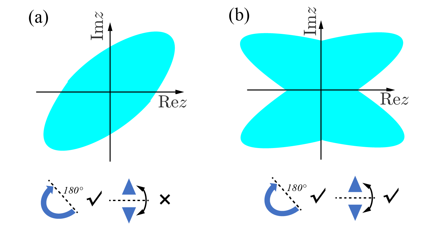
Figure 1: Symmetry of complex spectra (denoted by the colored region) for non-Hermitian random matrices. (a) Seven symmetry classes in the Altland-Zirnbauer₀ (AZ₀) classification. The complex spectrum is invariant under reflection about the spectral origin but not under reflection about the real or imaginary axis, resulting in the point group symmetry C₂. (b) Twenty-one symmetry classes beyond the AZ₀ classification. The complex spectrum is invariant under reflections about both real and imaginary axes, indicating the point group symmetry D₂.

In the first group, symmetry classes involve TRS^†, PHS, and SLS, but do not involve symmetries associated with complex or Hermitian conjugation. TRS^†, PHS, and SLS lead to the tenfold classification in Table 2 different from the AZ^† classification in Table 1. Here, we call this additional tenfold classification Altland-Zirnbauer₀ (AZ₀) classification since it is concerned with the spectral origin. Besides the three symmetry classes (i.e., classes A, AI^†, and AII^†) that only involve TRS^† and are counted before, the seven symmetry classes (i.e., classes AIII^†, BDI₀, CII₀, D, C, CI₀, and DIII₀) are in the first group. Owing to PHS, SLS, or both of them, which maps an eigenvalue $z$ to another eigenvalue $-z$, the complex spectra of generic matrices in any of these symmetry classes are invariant under the reflection about the spectral origin and hence respect the point group symmetry C₂ [see a schematic in Fig. 1 (a)]. Away from the origin, the spectral statistics depend solely on TRS^† since PHS and SLS merely create opposite-sign pairs of eigenvalues, $\left(z,-z\right)$. This is also the case for non-zero real or purely imaginary eigenvalues. Around the origin, by contrast, even PHS and SLS change the spectral correlations and lead to unique spectral statistics, as shown below. If a matrix $H$ belongs to one of these seven symmetry classes, $e^{\text{i}\phi}H$ also belongs to the same symmetry class for arbitrary $\phi\in\mathbb{R}$ (see Table 2).

The remaining $28-7=21$ symmetry classes are in the second group and involve at least one of TRS, PHS^†, CS, and pH, as summarized in Table 3. These symmetries accompany complex or Hermitian conjugation and hence map an eigenvalue $z$ to $z^{*}$ or $-z^{*}$. In these classes, SLS, PHS, or both of them also exist. Consequently, the real or imaginary axis exhibits higher symmetry than generic points, and the spectral origin exhibits even higher symmetry. Owing to the combination of these symmetries, $H$ does not necessarily belong to the same symmetry class as $e^{\text{i}\phi}H$ for generic $\phi\in\mathbb{R}$, in contrast to the AZ₀ symmetry classification. Rather, complex spectra of generic non-Hermitian matrices in these 21 symmetry classes are invariant under the reflections about the real and imaginary axes, and hence respect the point group symmetry D₂ [see a schematic in Fig. 1 (b)].

Below, we comprehensively study the spectral statistics around the origin—hard-edge statistics—of non-Hermitian random matrices in all the AZ₀ symmetry classes (Sec. III), as well as the other 21 symmetry classes with a particular focus on three typical classes (classes BDI, CI, and AII + $\mathcal{S}_{+}$) (Sec. IV). Through these analyses, we complete the classification of the universal spectral statistics of non-Hermitian random matrices in the 38-fold symmetry classes.

Table 2: Altland-Zirnbauer₀ (AZ₀) classification of non-Hermitian random matrices based on time-reversal symmetry^† (TRS^†), particle-hole symmetry (PHS), and sublattice symmetry (SLS). The column “Equivalent class” shows the equivalent symmetry classes in Ref. [46]. In the columns “TRS^†” and “PHS”, the entry “$\pm 1$” specifies the sign of the anti-unitary symmetry, and “$0$” means its absence. The density $\rho(|z|)$ of the modulus of eigenvalues and the level-ratio distribution $p_{r}(r)$ [Eq. (11)] share the same small-argument behaviors, which are summarized in the columns “$\rho(|z|)$ and $p_{r}(|z|)$”. The mean values $\langle r\rangle$ and $\langle\cos\theta\rangle$ of random matrices are summarized, where $re^{\text{i}\theta}$ is the level ratio around the spectral origin. The statistics are obtained by diagonalizing $10^{7}$ realizations of $128\times 128$ random matrices. The numbers in the parentheses denote standard deviations.

Class	Equivalent class	TRS†	PHS	SLS	$\rho(|z|)$ and $p_{r}(|z|)$	$\left\langle r\right\rangle$	$\left\langle\cos\theta\right\rangle$
A	-	$0$	$0$	$0$	-	-	-
AI†	-	$+1$	$0$	$0$	-	-	-
AII†	-	$-1$	$0$	$0$	-	-	-
AIII†	A + $\mathcal{S}$	$0$	$0$	$1$	$-|z|^{3}\ln|z|$	0.6357(5)	0.5391(7)
BDI0	D + $\mathcal{S}_{+}$, AI† + $\mathcal{S}_{+}$	$+1$	$+1$	$1$	$|z|$	0.5778(6)	0.5681(7)
CII0	C + $\mathcal{S}_{+}$, AII† + $\mathcal{S}_{+}$	$-1$	$-1$	$1$	$|z|^{3}$	0.6623(5)	0.5147(7)
D	-	$0$	$+1$	$0$	$|z|$	0.5411(6)	0.5524(7)
C	-	$0$	$-1$	$0$	$|z|^{3}$	0.6746(5)	0.5343(7)
CI0	C + $\mathcal{S}_{-}$, AI† + $\mathcal{S}_{-}$	$+1$	$-1$	$1$	$-|z|^{3}\ln|z|$	0.6708(5)	0.5589(7)
DIII0	D + $\mathcal{S}_{-}$, AII† + $\mathcal{S}_{-}$	$-1$	$+1$	$1$	$-|z|^{3}\ln|z|$	0.5950(6)	0.5252(7)

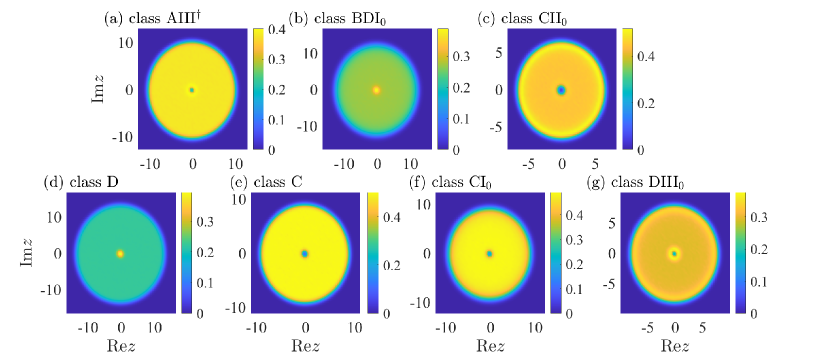
Figure 2: Density of complex eigenvalues of non-Hermitian random matrices in the Gaussian ensemble within the AZ₀ classification. In each symmetry class, the result is obtained by $10^{7}$ samples of $128\times 128$ random matrices. In classes (c) CII₀ and (g) DIII₀, all eigenvalues are twofold degenerate, and we only count the degenerate pairs once when calculating the density.

III Non-Hermitian random matrices in the AZ₀ classification

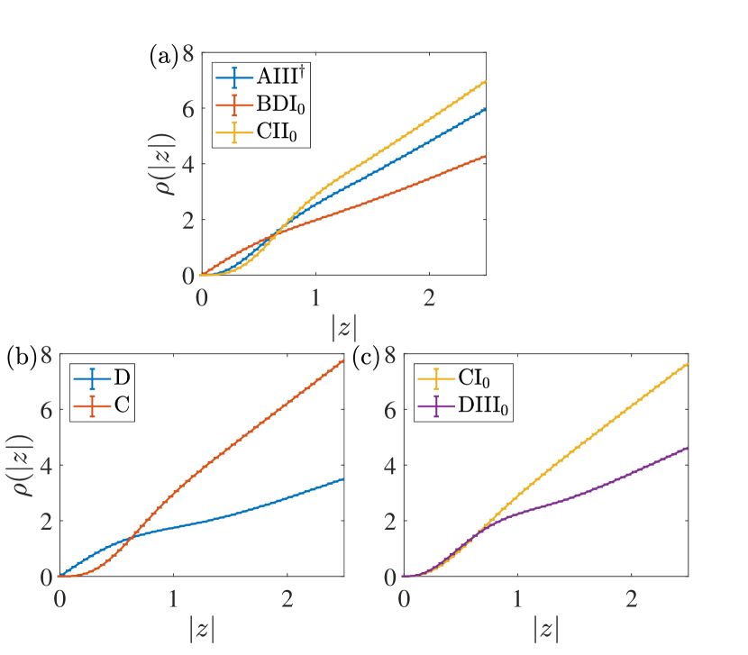
Figure 3: Density $\rho(|z|)$ of the modulus of complex eigenvalues of non-Hermitian random matrices in the Gaussian ensemble within the AZ₀ classification. (a) Classes AIII^† , BDI₀, and CII₀. (b) Classes D and C. (c) Classes CI₀ and DIII₀.

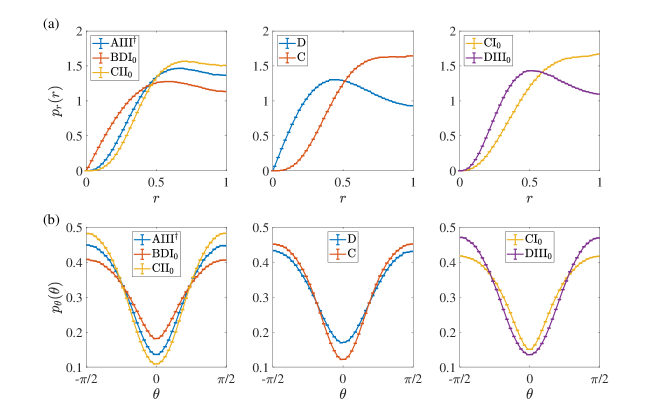
Figure 4: (a) Radial distributions $p_{r}(r)$ and (b) angular distributions $p_{\theta}(\theta)$ of the complex level ratio $re^{\text{i}\theta}$ [Eq. (11)] around the spectral origin for the seven symmetry classes in the AZ₀ classification. The error bars represent one standard deviation evaluated by the bootstrap method [114].

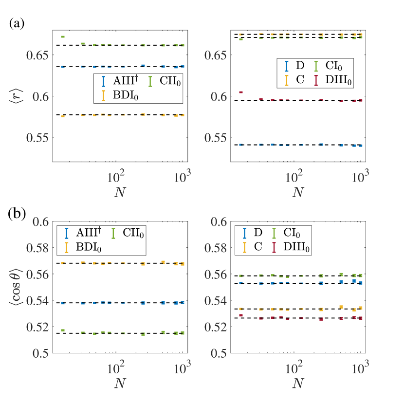
Figure 5: Mean values (a) $\left\langle r\right\rangle$ and (b) $\left\langle\cos\theta\right\rangle$ [Eq. (11)] as functions of the matrix size $N$. For each symmetry class and each matrix size, the number of diagoanlized samples is $N_{\rm sample}=10^{7},10^{6},2\times 10^{5}$ for $N=128$, $N<128$, $N>128$, respectively. The error bars represent one standard deviation. The dashed lines denote the mean values obtained by matrices with $N=128$.

We consider non-Hermitian random matrices in the seven symmetry classes within the AZ₀ classification (Table 2). Specifically, we take the Gaussian ensemble with the probability density function

$$p(H)\propto e^{-\beta\,{\rm Tr}\,(H^{\dagger}H)}$$ (8)

with a positive constant $\beta>0$. We follow the terminology in the AZ classification: classes AIII^†, BDI₀, and CII₀ are categorized as chiral symmetry classes, and classes D, C, CI₀, and DIII₀ are categorized as BdG classes. The explicit forms of non-Hermitian random matrices in each symmetry class are enumerated in Appendix A.

Similar to Hermitian random matrix theory [14], the total number $\nu d_{E}$ of topologically protected exact zero modes can manifest themselves and influence the level statistics around the origin in some symmetry classes. Here, $d_{E}$ refers to the degrees of degeneracy of generic eigenvalues: $d_{E}=2$ in the presence of TRS^† with the negative sign $-1$ (i.e., classes AIII^†, CII₀, and DIII₀) and $d_{E}=1$ otherwise. Specifically, a non-Hermitian random matrix $H$ in class D ($H^{\rm T}=-H$) has $\nu d_{E}=1$ zero mode if the matrix dimension of $H$ is odd. A non-Hermitian random matrix $H$ in class DIII₀ ($H^{\rm T}=-H$ and $\sigma_{y}H^{\rm T}\sigma_{y}=H$) has $\nu d_{E}=2$ zero modes if the matrix dimension of $H$ is $4n+2$ ($n\in\mathbb{Z}$). For non-Hermitian random matrices in classes AIII^†, BDI₀, and CII₀, on the other hand, $\nu d_{E}$ equals the difference between the numbers of positive and negative eigenvalues of the symmetry operator $\mathcal{S}$. While random matrices having such zero modes can be physically relevant, for example, to non-Hermitian superconductors with vortices [115, 116], dissipative SYK-type models [117], and QCD with topological charges [19], we focus on random matrices with $\nu d_{E}=0$ in this work.

We numerically diagonalize $10^{7}$ samples of $N\times N$ ($N=128$) non-Hermitian random matrices in each symmetry class. Let $z_{1}$ be the eigenvalue with the smallest modulus. We normalize eigenvalues such that $\langle|z_{1}|\rangle=1$, where $\langle\cdot\rangle$ denotes the average over the disorder ensemble. After the ensemble average, the density of complex eigenvalues does not depend on the phases of eigenvalues but only on their modulus (Fig. 2). It is rotationally invariant with respect to the origin and exhibits spectral U(1) rotation symmetry. This spectral U(1) symmetry arises because the Gaussian ensemble includes $e^{\text{i}\phi}H$ with the same probability for arbitrary $\phi\in\mathbb{R}$. The eigenvalues are distributed almost uniformly in a circle except around the origin and boundary. In classes BDI₀ and D, the density of eigenvalues around the origin is non-zero and higher than that in the bulk, revealing the absence of level repulsion at the spectral origin. On the other hand, in classes AIII^†, CII₀, C, CI₀, and DIII₀, the density vanishes at the origin.

Notably, the small-$|z|$ behavior of the density of the modulus of eigenvalues $z_{i}$,

$$\rho\left(|z|\right)\equiv\sum_{i}\left\langle\delta\left(|z|-|z_{i}|\right)\right\rangle,$$ (9)

characterizes the different strength of level repulsion in different symmetry classes (Fig. 3). Among the three chiral symmetry classes, the descending order of $\rho(|z|)$ for $|z|\ll 1$ is classes BDI₀, AIII^†, and CII₀ [see Fig. 3 (a)]. Among the four BdG symmetry classes, for $|z|\ll 1$, $\rho(z)$ in class D is the largest, that in class C is the smallest, and those in classes CI₀ and DIII₀ are close to each other [see Figs. 3 (b) and (c)]. Note that the density $\rho(|z|)$ of the modulus differs from the density of eigenvalues in the complex plane by a Jacobian, and hence we have $\rho(|z|=0)=0$ even in the absence of the level repulsion for classes D and BDI₀. Fitting $\rho(|z|)$, we find the asymptotic behavior of $\rho(|z|)$ for $|z|\ll 1$ (also summarized in Table 2),

$$\rho(|z|)\propto\begin{cases}|z|&(\text{classes D and BDI}_{0})\,;\\ -|z|^{3}\ln|z|&(\text{classes AIII}^{\dagger}\text{, CI}_{0}\text{, and DIII}_{0})\,;\\ |z|^{3}&(\text{classes CII}_{0}\text{ and C})\,.\end{cases}$$ (10)

As also discussed above, the linear decay of $\rho(|z|)$ for classes D and BDI₀ does not originate from the level repulsion but solely from the integral measure along the angular direction. By contrast, the cubic decay (with a potential logarithmic correction) for the other symmetry classes indicates the level repulsion around the spectral origin. The power-law decay of $\rho(|z|)$ is explained by the analytic calculations of small matrices, as shown in Appendix B.

To further characterize the level correlations around the spectral origin, we introduce a new quantitative measure of the hard-edge statistics for non-Hermitian operators. Owing to PHS, SLS, or both of them, complex eigenvalues must appear in the opposite-sign pairs $\left(+z,-z\right)$. Let $\pm z_{1},\pm z_{2},\pm z_{3},\ldots$ be eigenvalues (or Kramers pairs of eigenvalues) of $H$ in the ascending order of the modulus (i.e., $\left|z_{1}\right|\leq\left|z_{2}\right|\leq\left|z_{3}\right|\leq\cdots$). We introduce the complex level ratio by

$$re^{\text{i}\theta}\equiv\pm\frac{z_{1}}{z_{2}}\qquad(r,\theta\in\mathbb{R}).$$ (11)

Notably, the complex level ratio does not depend on the normalization of the random-matrix ensemble. We characterize the level-ratio statistics by the distribution $p_{r}(r)$ of the module $r$ of the ratio and the distribution $p_{\theta}(\theta)$ of its angle (phase) $\theta$,

$$p_{r}(r) \equiv\left\langle\delta\left(r-\left|\frac{z_{1}}{z_{2}}\right|\right)\right\rangle,$$ (12)

$$p_{\theta}(\theta) \equiv\left\langle\delta\left(\theta-{\rm arg}\left(\frac{z_{1}}{z_{2}}\right)\right)\right\rangle,$$ (13)

where we have $r\in[0,1]$ and $\theta\in[-\pi/2,\pi/2)$ by definition. When the levels are uncorrelated, $z_{1}$ is uniformly distributed inside the circle $|z_{1}|\leq|z_{2}|$, resulting in

$$p_{r}(r)=2r,\quad p_{\theta}(\theta)=\frac{1}{\pi}.$$ (14)

In Sec. V.4, we show that such level-ratio statistics indeed appear in an integrable open quantum system.

For the random-matrix ensemble, both the radial distribution $p_{r}(r)$ and the angular (phase) distribution $p_{\theta}(\theta)$ take non-trivial forms owing to the level correlations between the level pairs $(+z_{1},-z_{1})$ and $(+z_{2},-z_{2})$. From the numerical diagonalization of $128\times 128$ random matrices, we obtain the radial distribution $p_{r}(r)$ and angular distribution $p_{\theta}(\theta)$ of the complex level ratio $re^{\text{i}\theta}$ (Fig. 4). In each symmetry class, the distributions $p_{r}(r)$ and $p_{\theta}(\theta)$ show characteristic behavior, significantly distinct from that of uncorrelated levels. The small-$r$ behavior of $p_{r}(r)$ is similar to the small-$|z|$ behavior of the density $\rho(|z|)$ of the modulus of eigenvalues in the same symmetry class. For example, among the three chiral symmetry classes, the descending order of $p_{r}(r)$ for $r\ll 1$ is the same as that of $\rho(|z|)$ for $|z|\ll 1$ [compare Fig. 3 (a) with Fig. 4 (a)]. Fitting $p_{r}(r)$ with $r\ll 1$, we find that $p_{r}(r)$ shows the same power-law decay as $\rho(|z|)$ in Eq. (10) and Table 2. The density $\rho(|z|)$ should be mostly contributed by $z_{1}$ for $|z_{1}|\ll 1$, leading to $r\propto|z_{1}|$. Consequently, the small-argument behaviors of both $\rho(|z|)$ and $p_{r}(r)$ are mainly determined by the level correlations between the eigenvalue pair $\left(+z_{1},-z_{1}\right)$ closest to the spectral origin, which underlies the similarity between $\rho(|z|)$ and $p_{r}(r)$. Moreover, the angular distributions $p_{\theta}(\theta)$ are unique in different symmetry classes and characterize the different universality classes [Fig. 4 (b)]. First, we have $p_{\theta}(\theta)=p_{\theta}(-\theta)$ since the matrix ensembles are invariant under complex conjugation, transforming $\theta$ to $-\theta$. Second, $p_{\theta}(\theta)$ reaches its minimum and maximum at $\theta=0$ and $\pi/2$, respectively. The pairs $\left(+z_{1},-z_{1}\right)$ and $\left(+z_{2},-z_{2}\right)$ tend to be oriented perpendicularly to each other rather than in parallel, revealing the presence of level correlations. We also obtain the analytic formulas of $p_{r}^{N=4}(r)$ and $p_{\theta}^{N=4}(\theta)$ for $4\times 4$ non-Hermitian random matrices in classes AIII^† and D, which show behavior consistent with large ones (see Appendix B).

The mean values $\langle r\rangle$ and $\langle\cos\theta\rangle$ of the complex level ratio $re^{\text{i}\theta}$ serve as useful quantitative indicators of the hard-edge statistics among the different universality classes. These values in each symmetry class are summarized in Table 2. Notably, the distribution of $r$ in each symmetry class should converge to a universal form for sufficiently large matrix sizes. To clarify this convergence, we utilize $\left\langle r\right\rangle$ and $\left\langle\cos\theta\right\rangle$ as functions of the matrix size $N$ and find that they already reach the convergence for $N\geq 128$ (see Fig. 5). A similar rapid convergence of the distribution of $\left|z_{1}\right|$ was also reported in Ref. [93]. In Sec V, we also compare the random-matrix behavior of the hard-edge statistics with the distributions of physical models, which further provides evidence of the universality.

In the literature, the distributions of the eigenvalue $z_{1}$ with the smallest modulus were mainly used to characterize the hard-edge statistics (see Ref. [118] for the Hermitian case and Ref. [93] for the non-Hermitian case, as well as the references therein). Our newly proposed distributions of the complex level ratios in Eq. (11) differ from those of $z_{1}$ in several aspects. The distribution of $re^{\text{i}\theta}$ does not only depend on the modulus $r$ but also on the phase $\theta$ and hence is more informative than that of $z_{1}$. Studying $p_{r}(r)$ and $p_{\theta}(\theta)$ does not require normalization while studying the distribution of $z_{1}$ requires normalization, for example, by the mean value of $|z_{1}|$. Furthermore, the distribution of $re^{\text{i}\theta}$ can be more effective in distinguishing between integrable and non-integrable models, as demonstrated in Sec. V.4.

IV Non-Hermitian random matrices beyond the AZ₀ and AZ^† classification

We consider non-Hermitian random matrices in the 21 symmetry classes beyond the AZ₀ and AZ^† classification. Similar to the previous analysis, we take the Gaussian ensemble in Eq. (8). The relevant symmetries of these classes are summarized in Table 3. We first study classes BDI, CI, and AII + $\mathcal{S}_{+}$ as representative classes, and later discuss all the other classes in a similar manner. In Appendix C, we provide additional characterization of the hard-edge statistics for these general symmetry classes.

IV.1 Classes BDI, CI, and AII + $\mathcal{S}_{+}$

Non-Hermitian random matrices in class BDI (CI) respect TRS with sign $+1$ and CS commuting (anti-commuting) with TRS. On the other hand, non-Hermitian random matrices in class AII + $\mathcal{S}_{+}$ respect TRS with sign $-1$ and SLS commuting with TRS. See Table 3, as well as Appendix A for explicit forms of non-Hermitian random matrices in each symmetry class. We numerically diagonalize $10^{7}$ samples of $N\times N$ ($N=256$) non-Hermitian random matrices in each of the three symmetry classes. In these symmetry classes, the combination of symmetries leads to quartets $\left(z,-z,z^{*},-z^{*}\right)$ of complex eigenvalues, and hence the spectrum exhibits D₂ symmetry [see Fig. 1 (b)]. In all the three symmetry classes, the eigenvalues are distributed almost uniformly in a circle in the complex plane, except around its origin, its circumference, and the real and imaginary axes. This observation is consistent with the symmetries of these random matrices since the spectral origin, as well as the real and imaginary axes, possesses higher symmetries than generic points in the bulk of the spectrum. In classes BDI and CI, a subextensive number of eigenvalues are real or purely imaginary; in class AII + $\mathcal{S}_{+}$, by contrast, all eigenvalues are complex [Figs. 6 (d)-(f)]. We find that the presence of real or purely imaginary eigenvalues is determined by the relevant symmetries on the real and imaginary axes.

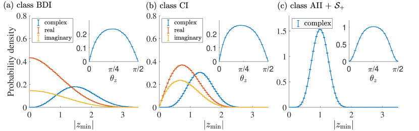
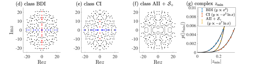
Figure 6: (a)-(c) Distributions of the eigenvalue $z_{\min}$ with the smallest modulus of non-Hermitian random matrices in classes BDI, CI, and AII + $\mathcal{S}_{+}$. The blue, orange, and yellow curves represent the radial distributions of $z_{\min}$ when it is complex, real, and purely imaginary, respectively. Inset: angular distribution of complex $z_{\min}$. The distributions are obtained by diagonalizing $10^{7}$ samples of $256\times 256$ random matrices in each symmetry class. (d)-(f) Eigenvalues of a single realization of a $256\times 256$ random matrix in each symmetry class. Complex, real, and purely imaginary eigenvalues are denoted by the black, blue, and red points, respectively. (g) Small-$|z_{\min}|$ behavior of the radial distributions of complex $z_{\min}$ in different symmetry classes, with the solid curves being fitting curves.

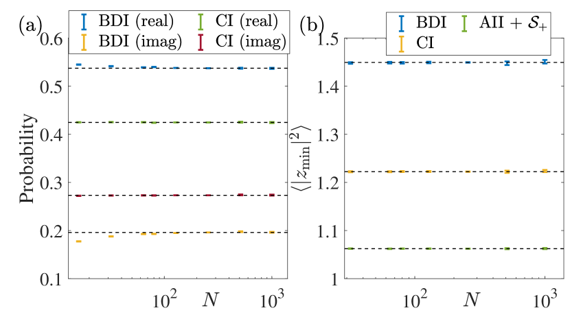
Figure 7: (a) Probability of the eigenvalue $z_{\rm min}$ with the smallest modulus being real or purely imaginary as functions of the matrix size $N$ in different symmetry classes. In class AII + $\mathcal{S}_{+}$, $z_{\rm min}$ is always complex. (b) $\langle|z_{\rm min}|^{2}\rangle$ as functions of the matrix size $N$ in different symmetry classes. The statistics are obtained by diagonalization of $N_{\rm sample}$ matrices for each class and size with $N_{\rm sample}=10^{7},10^{6},2\times 10^{5}$ for $N=256$, $N<256$, $N>256$, respectively. The error bars represent one standard deviation. The dashed lines denote the mean values obtained by matrices with $N=256$.

Table 3: Twenty-one symmetry classes of non-Hermitian random matrices beyond the AZ^† and AZ₀ classification. If $H$ belongs to the symmetry class in the column “Class ($H$)”, $\text{i}H$ belongs to the corresponding class in “Class ($\text{i}H$)”. If $H$ and $\text{i}H$ belong to the same symmetry class, the class is in bold. In the nomenclature of symmetry classes, $\mathcal{S}$ represents sublattice symmetry (SLS) and $\eta$ represents pseudo-Hermiticity (pH). The subscript of $\mathcal{S}_{\pm}$ or $\eta_{\pm}$ denotes whether SLS or pH commutes ($+$) or anti-commutes ($-$) with time-reveal symmetry (TRS), particle-hole symmetry (PHS), or chiral symmetry (CS). The first and second subscripts of $\mathcal{S}_{\pm\pm}$ denote the commutation ($+$) or anti-commutation ($-$) relations between SLS and TRS, and between SLS and PHS, respectively. In the columns “TRS”, “TRS^†”, “PHS”, and “PHS^†”, the entry “$\pm 1$” specifies the sign of the anti-unitary symmetry, and “$0$” means its absence. The column “$[\Gamma,\mathcal{S}]_{\pm}$=0” specifies whether CS $(\Gamma)$ and SLS $(\mathcal{S})$ commute ($+$) or anti-commute ($-$) with each other if both of them exist. The symmetry classes are categorized into different groups by the number ($N=0,2,4$) of anti-unitary symmetries. $z_{\rm min}$ denotes the eigenvalue with the smallest modulus. The level statistics around the spectral origin are characterized by $\langle|z_{\rm min}|^{2}\rangle$ and the probabilities of $z_{\min}$ being real or purely imaginary. If these probabilities equal each other within the range of statistical errors, they are in bold. The statistics are obtained by diagonalizing $10^{7}$ samples of $256\times 256$ random matrices for classes BDI, CI, and AII + $\mathcal{S}_{+}$ and diagonalizing $10^{6}$ samples of $256\times 256$ random matrices for the other symmetry classes.

Class ($H$)	Class ($\text{i}H$)	TRS	PHS	TRS†	PHS†	CS	SLS	pH	$[\Gamma,\mathcal{S}]_{\pm}$=0	$\langle|z_{\rm min}|^{2}\rangle$	Pr($z_{\min}\in\mathbb{R}$)	Pr($\text{i}z_{\min}\in\mathbb{R}$)
$N=0$
AIII + $\bm{\mathcal{S}_{+}}$	AIII + $\bm{\mathcal{S}_{+}}$	$0$	$0$	$0$	$0$	$1$	$1$	$1$	$+$	$1.1680(9)$	0.2279(5)	0.2280(5)
AIII + $\bm{\mathcal{S}_{-}}$	AIII + $\bm{\mathcal{S}_{-}}$	$0$	$0$	$0$	$0$	$1$	$1$	$1$	$-$	$1.2707(12)$	0.3336(5)	0.3334(5)
$N=2$
BDI	D + $\eta_{+}$	$+1$	$+1$	$0$	$0$	$1$	$0$	$0$		$1.4488(6)$	$0.5373(2)$	$0.1960(2)$
CI	C + $\eta_{-}$	$+1$	$-1$	$0$	$0$	$1$	$0$	$0$		$1.2223(4)$	$0.4247(2)$	$0.2732(2)$
DIII	D + $\eta_{-}$	$-1$	$+1$	$0$	$0$	$1$	$0$	$0$		$1.3390(13)$	$0$	$0.5419(5)$
CII	C + $\eta_{+}$	$-1$	$-1$	$0$	$0$	$1$	$0$	$0$		$1.0926(7)$	$0$	$0.2531(5)$
AI + $\bm{\mathcal{S}_{+}}$	AI + $\bm{\mathcal{S}_{+}}$	$+1$	$0$	$0$	$+1$	$0$	$1$	$0$		$1.3094(14)$	0.3885(5)	0.3894(5)
AI + $\mathcal{S}_{-}$	AII + $\mathcal{S}_{-}$	$+1$	$0$	$0$	$-1$	$0$	$1$	$0$		$1.2055(10)$	$0.5788(5)$	$0$
AII + $\bm{\mathcal{S}_{+}}$	AII + $\bm{\mathcal{S}_{+}}$	$-1$	$0$	$0$	$-1$	$0$	$1$	$0$		$1.0623(2)$	0	0
$N=4$
BDI + $\bm{\mathcal{S}_{++}}$	BDI + $\bm{\mathcal{S}_{++}}$	$+1$	$+1$	$+1$	$+1$	$1$	$1$	$1$	$+$	$1.4387(17)$	0.3502(5)	0.3504(5)
BDI + $\mathcal{S}_{--}$	DIII + $\mathcal{S}_{--}$	$+1$	$+1$	$-1$	$-1$	$1$	$1$	$1$	$+$	$1.2097(10)$	$0.5293(5)$	$0.0823(3)$
DIII + $\bm{\mathcal{S}_{++}}$	DIII + $\bm{\mathcal{S}_{++}}$	$-1$	$+1$	$+1$	$-1$	$1$	$1$	$1$	$+$	$1.1071(7)$	0	0
CI + $\bm{\mathcal{S}_{++}}$	CI + $\bm{\mathcal{S}_{++}}$	$+1$	$-1$	$-1$	$+1$	$1$	$1$	$1$	$+$	$1.2134(10)$	0.3655(5)	0.3661(5)
CI + $\mathcal{S}_{--}$	CII + $\mathcal{S}_{--}$	$+1$	$-1$	$+1$	$-1$	$1$	$1$	$1$	$+$	$1.1692(9)$	$0.4193(5)$	$0$
CII + $\bm{\mathcal{S}_{++}}$	CII + $\bm{\mathcal{S}_{++}}$	$-1$	$-1$	$-1$	$-1$	$1$	$1$	$1$	$+$	$1.0648(6)$	0.1022(4)	0.1025(4)
BDI + $\bm{\mathcal{S}_{+-}}$	BDI + $\bm{\mathcal{S}_{+-}}$	$+1$	$+1$	$-1$	$+1$	$1$	$1$	$1$	$-$	$1.3162(14)$	0.3878(5)	0.3881(5)
BDI + $\mathcal{S}_{-+}$	DIII + $\mathcal{S}_{-+}$	$+1$	$+1$	$+1$	$-1$	$1$	$1$	$1$	$-$	$1.4015(16)$	$0.6190(5)$	$0$
DIII + $\bm{\mathcal{S}_{+-}}$	DIII + $\bm{\mathcal{S}_{+-}}$	$-1$	$+1$	$-1$	$-1$	$1$	$1$	$1$	$-$	$1.2328(11)$	0.2797(5)	0.2802(5)
CI + $\bm{\mathcal{S}_{+-}}$	CI + $\bm{\mathcal{S}_{+-}}$	$+1$	$-1$	$+1$	$+1$	$1$	$1$	$1$	$-$	$1.2929(13)$	0.3684(5)	0.3692(5)
CI + $\mathcal{S}_{-+}$	CII + $\mathcal{S}_{-+}$	$+1$	$-1$	$-1$	$-1$	$1$	$1$	$1$	$-$	$1.1840(9)$	$0.4316(5)$	$0.2140(5)$
CII + $\bm{\mathcal{S}_{+-}}$	CII + $\bm{\mathcal{S}_{+-}}$	$-1$	$-1$	$+1$	$-1$	$1$	$1$	$1$	$-$	$1.0795(6)$	0	0

To characterize the level statistics around the spectral origin, we first consider the distribution $p_{\min}(z_{\rm min})$ of the eigenvalue $z_{\rm min}$ closest to the origin. To make $z_{\min}$ unique, we consider the distribution for ${\rm Re}\,z_{\min}\geq 0$ and ${\rm Im}\,z_{\min}\geq 0$. We normalize $z_{\min}$ such that $\left\langle|z_{\min}|\right\rangle=1$. Because of the possible presence of real and purely imaginary eigenvalues, the probability density $p_{\min}(z_{\min}=x+\text{i}y)$ of $z_{\min}$ is decomposed as

$$p_{\rm min}(z_{\min}=x+\text{i}y)$$

$$=p_{\rm min;r}(x)\delta(y)+p_{\rm min;i}(y)\delta(x)+p_{\rm min;c}(x,y)\,,$$ (15)

where $\delta(\cdot)$ is the Dirac delta function, and $p_{\rm min;r}(x)$, $p_{\rm min;i}(y)$, and $p_{\rm min;c}(x,y)$ represent the distributions of $z_{\min}$ when it is real, purely imaginary, and complex, respectively. The distribution $p_{\rm min}(z_{\min})$ is normalized by

$$\int_{0}^{\infty}dx\int_{0}^{\infty}dy~{}p_{\rm min}(x,y)=1,$$ (16)

and

$$\mathrm{Pr}\,(z_{\min}\in\mathbb{R}) \equiv\int_{0}^{\infty}dx~{}p_{\rm min;r}(x)\leq 1,$$ (17)

$$\mathrm{Pr}\,(\text{i}z_{\min}\in\mathbb{R}) \equiv\int_{0}^{\infty}dy~{}p_{\rm min;i}(y)\leq 1$$ (18)

represent the probability of $z_{\min}$ being real and purely imaginary, respectively. We provide both $\mathrm{Pr}\,(z_{\min}\in\mathbb{R})$ and $\mathrm{Pr}\,(\text{i}z_{\min}\in\mathbb{R})$ in Table 3. For $N\geq 256$, the probability of $z_{\min}$ being real or purely imaginary converges to a universal value characteristic to each symmetry class [Fig. 7 (a)]. Additionally, $\langle|z_{\min}|^{2}\rangle$ also converges to a universal value in each symmetry class for large $N$ [Fig. 7 (b)], which verifies the convergence of the statistics of $z_{\min}$ for $N\geq 256$.

We consider the radial distribution $p^{(r)}_{\rm min;c}(|z_{\rm min}|)$ for complex $z_{\min}\in\mathbb{C}$, given as

$$p^{(r)}_{\rm min;c}\,(|z_{\rm min}|)=\int_{0}^{\infty}dx\int_{0}^{\infty}dy~{}p_{\rm min;c}\,(x,y)$$

$$\qquad\qquad\qquad\qquad\qquad\times\delta\left(|z_{\rm min}|-\sqrt{x^{2}+y^{2}}\right).$$ (19)

Notably, $p^{(r)}_{\rm min;c}(|z_{\rm min}|)$ shows distinct behavior in each symmetry class [Figs. 6 (a)-(c), (g)]. In particular, their asymptotic behaviors for $|z_{\min}|\ll 1$ are given as

$$p^{(r)}_{\rm min;c}(|z_{\rm min}|)\propto\begin{cases}|z_{\min}|^{3}&\text{(class BDI)}\,;\\ -|z_{\min}|^{5}\ln|z_{\min}|&\text{(class CI)}\,;\\ -|z_{\min}|^{7}\ln|z_{\min}|&\text{(class AII}+\mathcal{S}_{+})\,.\\ \end{cases}$$ (20)

The joint probability distribution of complex eigenvalues for non-Hermitian random matrices in class AII + $\mathcal{S}_{+}$ with arbitrary $N$ was obtained previously [119]. In Appendix B, we verify that $4\times 4$ random matrices capture the same small-$|z_{\min}|$ behavior as that of large random matrices.

The distribution of complex $z_{\min}$ is qualitatively different from the distribution $p_{\rm min;r/i}(|z_{\min}|)$ of real or purely imaginary $z_{\min}$ (if exists) even in the same symmetry class. In fact, in class BDI, we have [Fig. 6 (a)]

$$p_{\rm min;r}(0)>0,\quad p_{\rm min;i}(0)>0.$$ (21)

In class CI, we have [Figs. 6 (b)]

$$p_{\rm min;r/i}(|z_{\rm min}|)\propto|z_{\rm min}|\quad\left(|z_{\min}|\ll 1\right).$$ (22)

They are significantly distinct from the small-$|z_{\min}|$ behavior of $p^{(r)}_{{\rm min};c}(|z_{\min}|)$. We provide an intuitive explanation for the stronger level repulsion for complex $z_{\rm min}$. As discussed before, all of $\pm z_{\min}$ and $\pm z_{\min}^{*}$ are eigenvalues. For complex $z_{\min}$, these four eigenvalues differ from each other and share the smallest modulus. By contrast, for real $z_{\min}$ ($z_{\min}=z_{\min}^{*}$) or purely imaginary $z_{\min}$ ($z_{\min}=-z_{\min}^{*}$), only the two different eigenvalues share the smallest modulus. Thus, for $|z_{\min}|\ll 1$, the number of eigenvalues closest to $z_{\min}$ is three for complex $z_{\rm min}$ and is one for real or purely imaginary $z_{\rm min}$, which leads to the different strength of level repulsion. In addition, we analytically calculate the hard-edge statistics for $4\times 4$ non-Hermitian random matrices in classes BDI in Appendix B, which also show distinct small-$|z_{\min}|$ behaviors for complex, real, and purely imaginary $z_{\min}$, consistent with those of large random matrices.

Furthermore, the angular distribution

$$p^{(\theta)}_{\rm min;c}\,(\theta_{z})=\int_{0}^{\infty}dx\int_{0}^{\infty}dy~{}p_{\rm min;c}\,(x,y)$$

$$\qquad\qquad\qquad\qquad\qquad\times\delta\left(\theta_{z}-\arctan\left(y/x\right)\right)$$ (23)

for complex $z_{\min}=|z_{\min}|e^{\text{i}\theta_{z}}$ [$\theta_{z}\in(0,\pi/2)$] shows characteristic behavior in each symmetry class [see the insets of Figs. 6 (a)-(c)]. In all the three symmetry classes, the distributions $p^{(\theta)}_{\rm min;c}(\theta_{z})$ vanish for $\theta_{z}\rightarrow 0$ or $\pi/2$ and get maximal for $\theta_{z}\simeq\pi/4$. This behavior is due to the level repulsion between $z_{\min}$ and $z_{\min}^{*}$ or $-z_{\min}^{*}$. Specifically, we have for $|\theta_{z}|\ll 1$

$$p^{(\theta)}_{\rm min;c}(\theta_{z})\propto\begin{cases}|\theta_{z}|&\text{(classes BDI and CI)}\,;\\ |\theta_{z}|^{2}&\text{(class AII}+\mathcal{S}_{+})\,.\\ \end{cases}$$ (24)

For $|\pi/2-\theta_{z}|\ll 1$, we also have

$$p^{(\theta)}_{\rm min;c}(\pi/2-\theta_{z})\propto\begin{cases}|\pi/2-\theta_{z}|&\text{(classes BDI and CI)}\,;\\ |\pi/2-\theta_{z}|^{2}&\text{(class AII}+\mathcal{S}_{+})\,.\\ \end{cases}$$ (25)

Notably, these linear or quadratic decays of $p^{(\theta)}_{\rm min;c}$ are reminiscent of the soft gap of the density $\rho_{c}(x+\text{i}y)$ of complex eigenvalues around the real axis in the presence of TRS or pH. In fact, in the presence of TRS with sign $+1$ or pH, we have $\rho_{c}(x+\text{i}y)\propto|y|$ for $|y|\ll 1$, and in the presence of TRS with sign $-1$, we have $\rho_{c}(x+\text{i}y)\propto|y|^{2}$ for $|y|\ll 1$, as summarized in Table 1 [55, 109, 111]. In both classes BDI and CI, non-zero real eigenvalues respect TRS with sign $+1$ while purely imaginary eigenvalues respect CS, equivalent to pH. The exponents in the power-law decay of $p_{\rm min;c}^{(\theta)}$ align with those of $\rho_{c}(x+\text{i}y)$. The difference between classes BDI and CI lies in the signs of PHS, not influencing symmetries of non-zero real or purely imaginary eigenvalues.

In class AII + $\mathcal{S}_{+}$, non-zero real eigenvalues respect TRS with sign $-1$ while non-zero purely imaginary eigenvalues respect PHS^† with sign $-1$, equivalent to TRS with sign $-1$ [51]. The exponent in the power-law decay of $p_{\rm min;c}^{(\theta)}$ also aligns with that of $\rho_{c}(x,y)$. It is also notable that $p^{(\theta)}_{\rm min;c}(\theta_{z})$ in class AII + $\mathcal{S}_{+}$ exhibits higher symmetry than those in classes BDI and CI. Because of the equivalence between TRS and PHS^†, if $H$ belongs to class AII + $\mathcal{S}_{+}$, $\text{i}H$ also belongs to class AII + $\mathcal{S}_{+}$, both of which occur with the same probability in the Gaussian ensemble. Consequently, the probability of $z$ being the eigenvalue with the smallest modulus is the same as that of $\text{i}z$. In combination with spectral D₂ symmetry due to TRS and SLS, the distribution of $z_{\rm min}$ should thus exhibit the point group symmetry D₄ after the ensemble average. This spectral D₄ symmetry requires $p^{(\theta)}_{\rm min;c}(\theta_{z})=p^{(\theta)}_{\rm min;c}(\pi/2-\theta_{z})$, consistent with the numerical results in the inset of Fig. 6 (c). On the other hand, such symmetry is absent in classes BDI and CI, and numerical results show that $p^{(\theta)}_{\rm min;c}(\theta_{z})$ equals $p^{(\theta)}_{\rm min;c}(\pi/2-\theta_{z})$ only approximately.

IV.2 General classes

Beyond the AZ₀ and AZ^† classification, we now investigate the remaining 18 symmetry classes. As indicators of the universal classes of the level statistics around the spectral origin, we use $\langle|z_{\rm min}|^{2}\rangle$ and the probability of $z_{\rm min}$ being real or purely imaginary, denoted by Pr($z_{\min}\in\mathbb{R}$) in Eq. (17) and Pr($\text{i}z_{\min}\in\mathbb{R}$) in Eq. (18), respectively. Since these indicators already reach the convergence for $256\times 256$ non-Hermitian random matrices in the three representative classes (see Fig. 7), we obtain these values in all the remaining 18 classes through the exact diagonalization of random matrices with the same size, as summarized in Table 3. We expect these values to be universal and characterize the universality classes of the complex spectral statistics. For the three representative classes, we shortly verify the universality also by comparison with physical models (see Table 5 in Sec. VI for details); the exhaustive verification for physical models in the other symmetry classes is left for future study.

In each symmetry class, the distributions of $z_{\min}$ exhibit the characteristic behavior. We find that whether Pr($z_{\min}\in\mathbb{R}$) is zero depends only on symmetries respected by the real axis (i.e., TRS, TRS^†, and pH), regardless of the other symmetries. These symmetries, comprising the AZ^† classification, also determine whether non-Hermitian random matrices in the AZ^† classification have real eigenvalues (see Sec. II and a summary in Table 1). For example, in the AZ^† classification, a random matrix in class AI + $\eta_{+}$ has TRS with sign $+1$ and TRS^† with sign $-1$, leading to a subextensive number of real eigenvalues (see Table 1). Correspondingly, classes BDI + $\mathcal{S}_{--}$, CI + $\mathcal{S}_{++}$, BDI + $\mathcal{S}_{+-}$, and CI + $\mathcal{S}_{-+}$ have the same signs of TRS and TRS^†, and non-Hermitian random matrices in these symmetry classes exhibit Pr$(z_{\min}\in\mathbb{R})\neq 0$ (see Table 3). Similarly, whether Pr($\text{i}z_{\min}\in\mathbb{R}$) is zero depends only on the symmetries respected by pure imaginary eigenvalues (i.e., PHS^†, TRS^†, and CS).

Another notable feature is spectral D₄ symmetry of the level statistics in some symmetry classes where $H$ and $\text{i}H$ belong to the same symmetry class. Such symmetry classes are shown in bold font in Table 3. When Pr$(z_{\min}\in\mathbb{R})$ and Pr$(\text{i}z_{\min}\in\mathbb{R})$ overlap within the range of statistical errors, they are also shown in bold font in Table 3. These two bold-font items consistently appear in the same rows in Table 3 due to the spectral D₄ symmetry of the distributions of $z_{\min}$, analogous to our discussion for class AII + $\mathcal{S}_{+}$.

V Open quantum systems in the AZ₀ classification

In quantum chaotic systems that respect PHS or SLS and are isolated from the environment, the spectral statistics around zero energy $E=0$ can be described by Hermitian random matrices in the same symmetry class (see, for example, Ref. [14] and references therein). Here, we calculate the density of complex eigenvalues and the distribution of the complex level ratios in Eq. (11) around the spectral origin of open quantum systems that respect PHS or SLS. We find that they are consistent with the statistics of non-Hermitian random matrices studied in Sec. III. As a comparison, we also study the level statistics of an integrable non-Hermitian many-body Hamiltonian with PHS.

V.1 Lindblad equation

When a quantum system is coupled to a Markovian environment, the time evolution of its reduced density matrix $\rho$ is described by the Lindblad equation [31, 32, 30]

$$\frac{d\rho}{dt} =\mathcal{L}(\rho)$$

$$\equiv-\text{i}[H,\rho]+\sum_{\mu}\left(L_{\mu}\rho L_{\mu}^{\dagger}-\frac{1}{2}\left\{L_{\mu}^{\dagger}L_{\mu},\rho\right\}\right)\,.$$ (26)

Here, $H$ is the Hamiltonian of the system that governs the unitary dynamics of $\rho$, and $L_{\mu}$’s represent dissipators originating from the coupling with the environment. The Lindbladian $\mathcal{L}$ is a superoperator that acts on the density matrix. Through the vectorization $\rho=\rho_{ij}\ket{i}\bra{j}\rightarrow\ket{\rho}=\rho_{ij}\ket{i}\ket{j}$, the density matrix can be mapped to a state in the double Hilbert space. Correspondingly, $\mathcal{L}$ becomes a non-Hermitian operator in the double Hilbert space, given as

$$\mathcal{L}=-\text{i}\left(H\otimes 1-1\otimes H^{*}\right)$$ (27)

$$+\sum_{\mu}\left[L_{\mu}\otimes L_{\mu}^{*}-\frac{1}{2}\left(L_{\mu}^{\dagger}L_{\mu}\otimes 1\right)-\frac{1}{2}\left(1\otimes L_{\mu}^{\rm T}L_{\mu}^{*}\right)\right]\,.$$

For a generic system with $N$ complex fermions, the dimension of the double Hilbert space is $(2^{N})^{2}=4^{N}$. Therefore, $\mathcal{L}$ is a $4^{N}\times 4^{N}$ operator, and numerical evaluation of its spectrum for larger $N$ costs computation time.

Notably, quadratic Lindbladians, comprising quadratic Hamiltonians and linear dissipators, effectively reduce to single-particle non-Hermitian Hamiltonians [120, 121], which facilitates numerical investigations of relatively larger systems. A non-interacting fermionic Hamiltonian and linear dissipators are generally given by

$$H=\frac{1}{2}\sum_{i,j=1}^{2N}\Psi_{i}^{\dagger}H_{ij}\Psi_{j},\quad L_{\mu}=\sum_{i=1}^{2N}l_{\mu\text{i}}\Psi_{i}\,,$$ (28)

in the Nambu basis ${\Psi}=(c_{1},\cdots,c_{N},c_{1}^{\dagger},\cdots,c_{N}^{\dagger})^{\rm T}$. By construction, the $2N\times 2N$ matrix $H$ respects PHS $H=-\tau_{x}H^{\rm T}\tau_{x}$, where $\tau_{x}$ is the Pauli matrix acting on the $(c,c^{\dagger})$ space. We define a $2N\times 2N$ matrix by

$$N_{ij}\equiv(l^{\rm T}l^{*})_{ij}=\sum_{\mu}l_{\mu i}l_{\mu j}^{*}\,,$$ (29)

and its particle-hole-symmetric combination

$$\Gamma\equiv\frac{1}{2}(N+\tau_{x}N^{\rm T}\tau_{x})\,.$$ (30)

Using $H$ and $\Gamma$, we can construct a $2N\times 2N$ single-particle non-Hermitian Hamiltonian

$$K\equiv H-\text{i}\Gamma\,.$$ (31)

From complex eigenvalues $\lambda_{i}$’s of this effective single-particle non-Hermitian Hamiltonian $K$, the $4^{N}$ eigenvalues of $\mathcal{L}$ are given as

$$\Lambda_{{\bm{i}}}=-2\text{i}\sum_{i=1}^{2N}n_{i}\lambda_{i}\,,$$ (32)

with $n_{i}=0$ or $1$. Notably, $K$ always satisfies PHS^†,

$$\tau_{x}K^{*}\tau_{x}=-K.$$ (33)

In this work, we consider $H$ with the conserved particle number, given by

$$H=\frac{1}{2}\begin{pmatrix}h&0\\ 0&-h^{\rm T}\end{pmatrix}\,.$$ (34)

The coupling with the environment is assumed to manifest itself in single-particle loss; the dissipators $L_{\mu}$ consist only of annihilation operators,

$$L_{\mu}=\sum_{i=1}^{N}l_{\mu\text{i}}c_{i}.$$ (35)

In such a case, the effective single-particle non-Hermitian Hamiltonian $K$ is block-diagonalized as

$$K=\frac{1}{2}\begin{pmatrix}h-\text{i}l^{\rm T}l^{*}&0\\ 0&-h^{\rm T}-\text{i}l^{\dagger}l\end{pmatrix}\,.$$ (36)

While PHS^† in Eq. (33) relates the two reduced blocks $h-\text{i}l^{\rm T}l^{*}$ and $-h^{\rm T}-\text{i}l^{{\dagger}}l=-(h-\text{i}l^{\rm T}l^{*})^{*}$, the reduced block $h-\text{i}l^{\rm T}l^{*}$ itself does not necessarily respect PHS^†. The symmetry of quadratic Lindbladians is determined solely by $h-\text{i}l^{\rm T}l^{*}$ without intrinsic PHS^†. Since $h$ is Hermitian and $l^{\rm T}l^{*}$ is positive semidefinite, complex eigenvalues $z_{i}$’s of $h-\text{i}l^{\rm T}l^{*}$ must satisfy the constraint

$${\rm Im}\,z_{i}\leq 0.$$ (37)

It was argued that quadratic Lindbladians cannot respect TRS, PHS, pH, or SLS since these symmetries violate this positivity constraint [94]. As discussed previously, TRS or pH (PHS or SLS) requires complex eigenvalues to appear in $\left(z,z^{*}\right)$ [$\left(z,-z\right)$] pairs, which is incompatible with Eq. (37). However, if we shift the Lindbladian by its trace, the traceless part is free from such constraints [122, 123, 96, 97]. In principle, the diagonal block of the traceless part, given as

$$h_{\rm eff}\equiv h-\text{i}l^{\rm T}l^{*}-\frac{1}{N}{\rm Tr}K$$ (38)

can respect any of the seven symmetries in Eqs. (1)-(7). Hereafter, we investigate the symmetry classes and the hard-edge statistics of the shifted quadratic Lindbladian, represented by the effective non-Hermitian Hamiltonian $h_{\rm eff}$.

Table 4: Mean values $\langle r\rangle$ and $\langle\cos\theta\rangle$ of non-Hermitian random matrices (RM) and Hamiltonians in Eqs. (43)-(45) and (V.3)-(V.3) in the AZ₀ classification, where $re^{\text{i}\theta}$ denotes the complex level ratio [Eq. (11)] around the spectral origin.

Class	$\langle r\rangle$ (RM)	$\langle r\rangle$ (Hamiltonian)	$\langle\cos\theta\rangle$ (RM)	$\langle\cos\theta\rangle$ (Hamiltonian)
AIII†	0.6357(1)	0.6357(5)	0.5381(1)	0.5391(7)
BDI0	0.5773(1)	0.5778(6)	0.5682(1)	0.5681(7)
CII0	0.6618(1)	0.6623(5)	0.5150(1)	0.5147(7)
D	0.5408(1)	0.5411(6)	0.5528(1)	0.5524(7)
C	0.6749(1)	0.6746(5)	0.5334(1)	0.5343(7)
CI0	0.6711(1)	0.6708(5)	0.5585(1)	0.5589(7)
DIII0	0.5949(1)	0.5950(6)	0.5265(1)	0.5252(7)

V.2 Quadratic Lindbladians

We study three prototypical models of quadratic Lindbladians in the AZ₀ classification. We consider the following non-interacting Hermitian Hamiltonians on the three-dimensional cubic lattice ${\bm{i}}\in\mathbb{Z}^{3}$ in the chiral symmetry classes (i.e., classes AIII, BDI, and CII):

$$H=\sum_{\left\langle{\bm{i}},{\bm{j}}\right\rangle}c_{{\bm{i}}}^{\dagger}t_{{\bm{i}},{\bm{j}}}c_{{\bm{j}}}+\text{H.c.}\,,$$ (39)

where the bracket $\left\langle{\bm{i}},{\bm{j}}\right\rangle$ represents the nearest neighboring sites. Each site contains only one orbital but can accompany the spin degree of freedom. We assume the periodic boundary conditions and the system size of $L^{3}$. For any hopping amplitude $t_{{\bm{i}},{\bm{j}}}$ and $L\in 2\mathbb{Z}$, the Hamiltonian respects SLS

$$\mathcal{S}H\mathcal{S}=-H$$ (40)

with $\mathcal{S}_{{\bm{i}},{\bm{j}}}\equiv\delta_{{\bm{i}},{\bm{j}}}(-1)^{({\bm{i}}_{x}+{\bm{i}}_{y}+{\bm{i}}_{z})}$. Depending on the choices of $t_{{\bm{i}},{\bm{j}}}$, $H$ realizes models in all three chiral symmetry classes, as follows. Let us first consider the cases without the spin degree of freedom:

• Class AIII.—Choose $t_{{\bm{i}},{\bm{j}}}=e^{\text{i}\theta_{{\bm{i}},{\bm{j}}}}$, where $\theta_{{\bm{i}},{\bm{j}}}\in\mathbb{R}$ is distributed uniformly and independently in $[0,2\pi)$. The Hamiltonian realizes the random flux model [124, 125] and is denoted by $H_{\rm AIII}$. The Hamiltonian $H_{\rm AIII}$ only respects SLS and hence belongs to class AIII.

• Class BDI.—Choose $t_{{\bm{i}},{\bm{j}}}$ to be real-valued and distributed $t_{{\bm{i}},{\bm{j}}}\in\mathbb{R}$ uniformly and independently in $[t-W/2,t+W/2]$. The Hamiltonian realizes the random hopping model [124, 125] and is denoted by $H_{\rm BDI}$. In addition to SLS, $H_{\rm BDI}$ respects TRS

  $$H_{\rm BDI}^{*}=H_{\rm BDI}$$ (41)

  and hence belongs to class BDI.

Consider next the case with the spin degree of freedom:

• Class CII.—Choose $2\times 2$ hopping matrices $t_{{\bm{i}},{\bm{j}}}$ that are distributed uniformly and independently on the Harr measure of SU(2) matrices. The Hamiltonian realizes the SU(2) model [126] and is denoted by $H_{\rm CII}$. In addition to SLS, $H_{\rm CII}$ respects TRS

  $$\sigma_{y}H_{\rm CII}^{*}\sigma_{y}=H_{\rm CII}$$ (42)

  and hence belongs to class CII.

These models were originally proposed for solid-state materials but also found realizations in synthetic materials such as cold atoms and photonic systems [127, 128, 129, 130]. The coupling between cold atoms can be designed to respect chiral symmetry [128], and the hopping $t_{{\bm{i}},{\bm{j}}}$ can be controlled by synthetic gauge fields [131, 132].

We introduce the single-particle loss by dissipators that consist of a linear combination of annihilation operators [133, 48, 134, 51]. For each Hamiltonian $H$, we choose the following linear dissipators such that the relevant symmetries are respected:

• Class AIII^†.—For $H_{\rm AIII}$, we introduce the dissipators as $L_{{\bm{i}}}=\sqrt{{\gamma}}(c_{{\bm{i}}}+\text{i}c_{{\bm{i}}+{\bm{e}}_{z}})$ (${\bm{i}}\in\mathbb{Z}^{3}$).

• Class BDI₀.—For $H_{\rm BDI}$, we introduce the dissipators as $L_{{\bm{i}}}=\sqrt{{\gamma}}(c_{{\bm{i}}}+c_{{\bm{i}}+{\bm{e}}_{z}})$ (${\bm{i}}\in\mathbb{Z}^{3}$).

• Class CII₀.—For $H_{\rm CII}$, we introduce the dissipators as $L_{{\bm{i}}\sigma}=\sqrt{{\gamma}}(c_{{\bm{i}}\sigma}+c_{({\bm{i}}+{\bm{e}}_{z})\sigma})$ (${\bm{i}}\in\mathbb{Z}^{3},\sigma=\uparrow,\downarrow$).

In all the cases, $\gamma\geq 0$ denotes the dissipative coupling strength between the system and environment. The dissipative coupling is assumed to be identical among different sites and maintain translation invariance. The effective non-Hermitian Hamiltonians in Eq. (38) are given as

$$h_{\rm eff}^{\rm AIII^{\dagger}} =H_{\rm AIII}+\gamma\sum_{{\bm{i}}}\left(c_{{\bm{i}}+e_{z}}^{\dagger}c_{{\bm{i}}}-c_{{\bm{i}}}^{\dagger}c_{{\bm{i}}+{\bm{e}}_{z}}\right)\,,$$ (43)

$$h_{\rm eff}^{\rm BDI_{0}} =H_{\rm BDI}-\text{i}\gamma\sum_{{\bm{i}}}\left(c_{{\bm{i}}+e_{z}}^{\dagger}c_{{\bm{i}}}+c_{{\bm{i}}}^{\dagger}c_{{\bm{i}}+{\bm{e}}_{z}}\right)\,,$$ (44)

$$h_{\rm eff}^{\rm CII_{0}} =H_{\rm CII}+\gamma\sum_{{\bm{i}}}\left(c_{{\bm{i}}+e_{z}}^{\dagger}\sigma_{0}c_{{\bm{i}}}-c_{{\bm{i}}}^{\dagger}\sigma_{0}c_{{\bm{i}}+{\bm{e}}_{z}}\right)\,,$$ (45)

respectively. These effective non-Hermitian Hamiltonians still respect SLS and TRS^† with the same symmetry operators. In fact, we have

$$\left(h_{\rm eff}^{\rm BDI_{0}}\right)^{\rm T}=h_{\rm eff}^{\rm BDI_{0}},\quad\sigma_{y}\left(h_{\rm eff}^{\rm CII_{0}}\right)^{\rm T}\sigma_{y}=h_{\rm eff}^{\rm CII_{0}}.$$ (46)

Thus, $h_{\rm eff}^{\rm AIII^{\dagger}}$, $h_{\rm eff}^{\rm BDI_{0}}$, and $h_{\rm eff}^{\rm CII_{0}}$ belong to symmetry classes AIII^†, BDI₀, and CII₀, respectively.

We diagonalize these effective non-Hermitian Hamiltonians numerically, with the parameters chosen as follows: (i) Class AIII^† ($h_{\rm eff}^{\rm AIII^{\dagger}}$).—$t_{{\bm{i}},{\bm{j}}}=e^{\text{i}\theta_{{\bm{i}},{\bm{j}}}}$ with $\theta_{{\bm{i}},{\bm{j}}}\in[0,2\pi)$, $\gamma=0.1$, and $L=18$; (ii) Class BDI₀ ($h_{\rm eff}^{\rm BDI_{0}}$).—$t=1$, $W=1.6$, $\gamma=0.1$, and $L=18$; (iii) Class CII₀ ($h_{\rm eff}^{\rm CII_{0}}$).—$t_{{\bm{i}},{\bm{j}}}$’s are random SU(2) matrices; $\gamma=0.4$ and $L=12$. For each class, we diagonalize $2\times 10^{5}$ samples in the disorder ensemble. Figures 8 (a), (c), and (e) show the distributions of complex eigenvalues for a single realization of each Hamiltonian. The full complex spectra deviate from the circular law of non-Hermitian random matrices [106, 135] and are generally non-universal. The range of each spectrum along the imaginary-axis direction is much smaller than that along the real-axis direction because of the small dissipation strength $\gamma$.

We investigate the spectral properties around the origin and demonstrate that they conform to the universal hard-edge statistics determined solely by symmetry. We normalize the eigenvalues of the Hamiltonians such that $\langle|z_{1}|\rangle=1$, where $z_{1}$ denotes the complex eigenvalue with the smallest modulus. After the ensemble average, the density of complex eigenvalues around the spectral origin does not depend on the phases but only on the modulus, and hence exhibits spectral U(1) rotation symmetry [Figs. 8 (b), (d), and (f)]. For the Hamiltonians in different symmetry classes, $\rho(|z|)$’s show distinct behavior consistent with the characteristic forms of non-Hermitian random matrices in the corresponding symmetry classes [Fig. 9 (a)]. The complex level ratios $re^{\text{i}\theta}\equiv z_{1}/z_{2}$ in Eq. (11) around the spectral origin also obey the same distributions of non-Hermitian random matrices in the same symmetry class [Figs. 9 (b) and (c)]. To further validate this consistency, in Table 4, we compare $\langle r\rangle$ and $\langle\cos\theta\rangle$ of the effective non-Hermitian Hamiltonians (and also those studied in Sec. V.3) and non-Hermitian random matrices. In each symmetry class, the corresponding statistical quantities overlap with each other within two standard deviations. Our results demonstrate the universality of the hard-edge statistics of non-Hermitian random matrices and reveal the chaotic nature of the quadratic Lindbladians.

As also discussed above, the complex spectra around the origin exhibit U(1) rotation symmetry even for the physical models. Notably, this spectral U(1) symmetry of the ensemble-average density does not arise from the original symmetry of the disorder ensemble of the Hamiltonians but from the chaotic behavior. In fact, unlike the Gaussian ensemble of random matrices, $e^{\text{i}\phi}h_{\rm eff}^{\rm X}$ ($\rm X=AIII^{\dagger},BDI_{0},CII_{0}$) does not belong to the same disorder ensemble of $h_{\rm eff}^{\rm X}$ for generic $\phi\in\mathbb{R}$. Nevertheless, its hard-edge statistics can still be described by random matrices, resulting in the emergence of the spectral U(1) symmetry. Notably, the spectra away from the origin, especially spectral boundaries [see Fig. 8 (a), (c), and (e)], do not respect the U(1) rotation symmetry. Thus, in such systems, an energy threshold $E_{c}\geq 0$ should exist, akin to the Thouless energy [136], such that the spectra are well described by the random matrices for $|z|\leq E_{c}$. In the study of closed quantum systems, the Thouless energy was shown to satisfy $E_{c}\propto L^{-2}$ [137], exhibiting the same order as the mean level spacing of a two-dimensional system. In our open quantum systems studied here, $E_{c}$ is at least larger than $2\langle|z_{1}|\rangle$, while an accurate estimate of $E_{c}$ is left for future study. It should also be noted that the emergent spectral U(1) symmetry, as well as the universality of the hard-edge statistics, is exact only in the infinite-size limit $L\rightarrow\infty$.

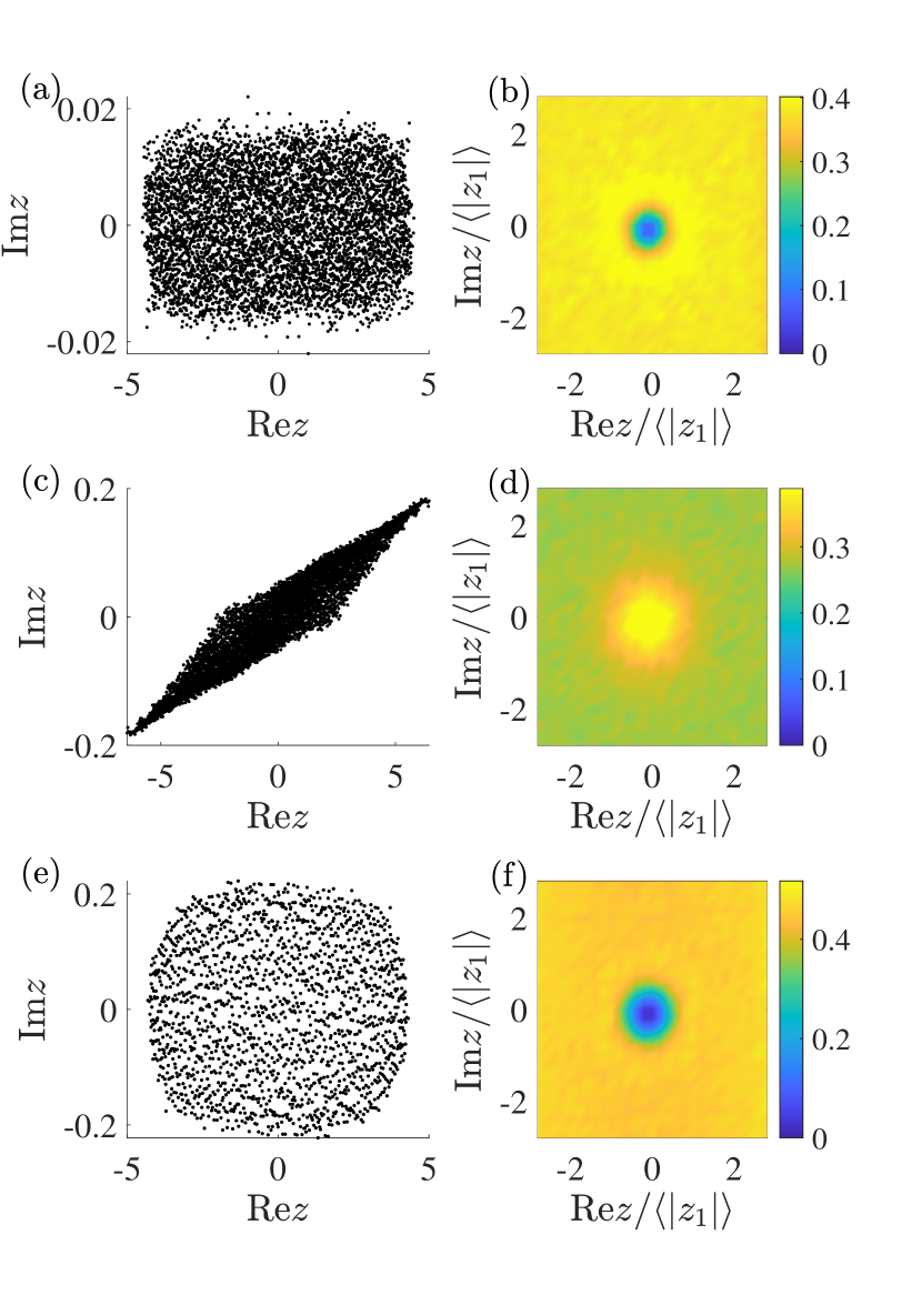
Figure 8: Complex eigenvalues of single realizations of the effective non-Hermitian Hamiltonians in Eqs. (43)-(45) of the quadratic Lindbladians in classes (a) AIII^†, (c) BDI₀, and (e) CII₀. (b), (d), (f) Ensemble average of the density of complex eigenvalues around the spectral origin of the same Hamiltonians as the left subfigures.

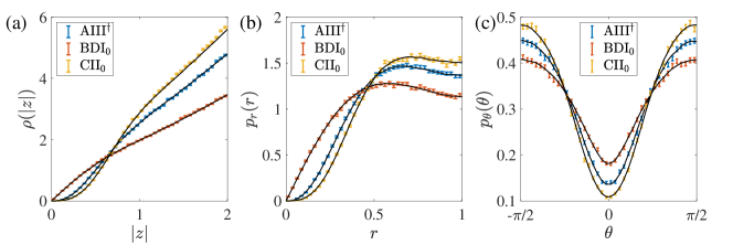
Figure 9: Hard-edge statistics of the effective non-Hermitian Hamiltonians in Eqs. (43)-(45) of the quadratic Lindbladians in classes AIII^†, BDI₀, and CII₀. (a) Density $\rho(|z|)$ of the modulus of complex eigenvalues. (b) Radial distributions $p_{r}(r)$ and (c) angular distributions $p_{\theta}(\theta)$ of the complex level ratios $re^{\text{i}\theta}$ [Eq. (11)] around the spectral origin. The colored points with the error bars refer to the Hamiltonians, and the black solid lines are obtained by non-Hermitian random matrices in the same symmetry classes.

V.3 Non-Hermitian superconductors

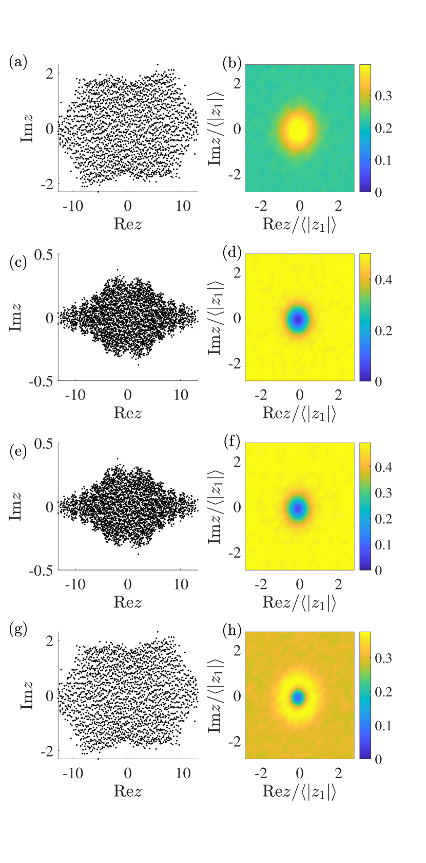
Figure 10: Complex eigenvalues of single realizations of the Hamiltonians in Eqs. (V.3)-(V.3) of non-Hermitian superconductors in classes (a) D, (c) C, (e) CI₀, and (g) DIII₀. (b), (d), (f), (h) Ensemble average of the density of complex eigenvalues around the spectral origin of the same Hamiltonians as the left subfigures.

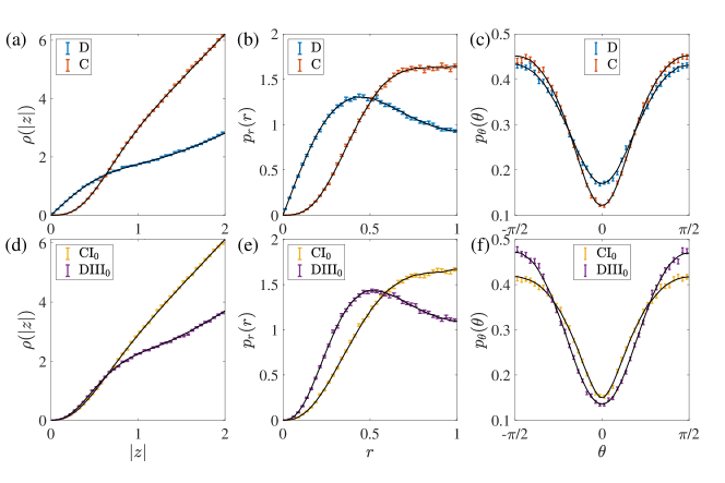
Figure 11: Hard-edge statistics of the Hamiltonians in Eqs. (V.3)-(V.3) of non-Hermitian superconductors in classes D, C, CI₀, and DIII₀. (a) Density $\rho(|z|)$ of the modulus of eigenvalues. (b) Radial distributions $p_{r}(r)$ and (c) angular distributions $p_{\theta}(\theta)$ of the complex level ratios $re^{\text{i}\theta}$ [Eq. (11)] around the spectral origin. The colored points with the error bars refer to the Hamiltonians, and the black solid curves are obtained by non-Hermitian random matrices in the corresponding symmetry classes.

Superconductors with energy gain and loss are one of the most intensively studied systems in the field of non-Hermitian physics [100, 46]. Superconductors attached to leads or reservoirs are also effectively described by non-Hermitian Hamiltonians [98, 99, 102]. In the following, we study four prototypical models of non-Hermitian superconductors that belong to classes D, C, CI₀, and DIII₀ in the AZ₀ classification and demonstrate its dissipative quantum chaos described by non-Hermitian random matrices with symmetry.

(i) For symmetry class D, we introduce an energy gain and loss into a two-dimensional $p$-wave superconductor,

$$H_{\rm D}=2\sum_{{\bm{i}}}\left[\left(\epsilon^{r}_{{\bm{i}}}+\text{i}\epsilon^{i}_{{\bm{i}}}-\mu\right)c_{{\bm{i}}}^{\dagger}c_{{\bm{i}}}+\left(te^{\text{i}\phi}c_{{\bm{i}}+{\bm{e}}_{x}}^{\dagger}c_{{\bm{i}}}\right.\right.$$

$$\left.\left.+tc_{{\bm{i}}+{\bm{e}}_{y}}^{\dagger}c_{{\bm{i}}}+\text{i}\Delta c_{{\bm{i}}+{\bm{e}}_{x}}c_{{\bm{i}}}+\Delta c_{{\bm{i}}+{\bm{e}}_{y}}c_{{\bm{i}}}+{\rm H.c.}\right)\right]\,.$$ (47)

Here, $\epsilon^{r}_{{\bm{i}}}$ and $\epsilon^{i}_{{\bm{i}}}$ are a random chemical potential and random energy gain or loss that are distributed distribute uniformly and independently in $[-W_{1}/2,W_{1}/2]$ and $[-W_{2}/2,W_{2}/2]$, respectively. Additionally, $te^{\text{i}\phi}$ and $t$ represent the hopping amplitudes, and $\Delta$ and $\text{i}\Delta$ are the $p$-wave superconducting paring potentials. The phase $e^{\text{i}\phi}$ of the hopping term can originate from a spatial modulation of the superconducting phase. In fact, with a gauge transformation $c_{{\bm{i}}}\rightarrow e^{\text{i}{\bm{i}}_{x}\phi}c_{{\bm{i}}}$, the hopping phase can be eliminated [138], and the paring terms change as $\text{i}\Delta c_{{\bm{i}}+{\bm{e}}_{x}}c_{{\bm{i}}}\rightarrow\text{i}\Delta e^{\text{i}(2{\bm{i}}_{x}\phi+\phi)}c_{{\bm{i}}+{\bm{e}}_{x}}c_{{\bm{i}}}$ and $\Delta c_{{\bm{i}}+{\bm{e}}_{y}}c_{{\bm{i}}}\rightarrow\Delta e^{\text{i}(2{\bm{i}}_{x}\phi)}c_{{\bm{i}}+{\bm{e}}_{y}}c_{{\bm{i}}}$. In the Nambu basis $\Psi_{{\bm{i}}}=(c_{{\bm{i}}},c_{{\bm{i}}}^{\dagger})^{\rm T}$, the Hamiltonian is written as

$$H_{\rm D} =\sum_{{\bm{i}}}\left\{\left(\epsilon^{r}_{{\bm{i}}}+\text{i}\epsilon^{i}_{{\bm{i}}}-\mu\right)\Psi_{{\bm{i}}}^{\dagger}\tau_{z}\Psi_{{\bm{i}}}\right.$$

$$\left.+\left[\Psi_{{\bm{i}}+{\bm{e}}_{x}}^{\dagger}(t\cos\phi\tau_{z}+\text{i}t\sin\phi\tau_{0}+\text{i}\Delta\tau_{x})\Psi_{{\bm{i}}}\right.\right.$$

$$\left.\left.+\Psi_{{\bm{i}}+{\bm{e}}_{y}}^{\dagger}(t\tau_{z}+\text{i}\Delta\tau_{y})\Psi_{{\bm{i}}}+{\rm H.c.}\right]\right\}\,.$$ (48)

This Hamiltonian $H_{\rm D}$ satisfies

$$\tau_{x}H_{\rm D}^{\rm T}\tau_{x}=-H_{\rm D},$$ (49)

and hence belongs to class D.

(ii) For symmetry class C, we introduce a random imbalanced $s$-wave pairing potential into a three-dimensional superconductor with conserved spin,

$$H_{\rm C} =\sum_{{\bm{i}}}\left\{\Psi_{{\bm{i}}}^{\dagger}\left[(\epsilon_{{\bm{i}}}-\mu)\tau_{z}+\text{i}\Delta^{s}_{{\bm{i}}}\tau_{y}\right]\Psi_{{\bm{i}}}\right.$$

$$\left.+\left[\Psi_{{\bm{i}}+{\bm{e}}_{z}}^{\dagger}(t\cos\phi\tau_{z}+\text{i}t\sin\phi\tau_{0}+\text{i}\Delta\tau_{y})\Psi_{{\bm{i}}}\right.\right.$$

$$\left.\left.+\sum_{\mu=x,y}\Psi_{{\bm{i}}+{\bm{e}}_{\mu}}^{\dagger}(t\tau_{z}+\Delta\tau_{x})\Psi_{{\bm{i}}}+{\rm H.c.}\right]\right\}\,$$ (50)

with the Nambu basis $\Psi_{{\bm{i}}}=(c_{\uparrow},c_{\downarrow}^{\dagger})$. Here, $\epsilon_{{\bm{i}}}$ is a random potential distributed uniformly and independently in $[-W_{1}/2,W_{1}/2]$. $t$ and $\phi$ characterize the hopping amplitudes, $\Delta\in\mathbb{R}$ represents a Hermitian pairing potential, and $\Delta^{s}_{{\bm{i}}}\in\mathbb{R}$ represents the random imbalanced $s$-wave paring potential [139, 140, 141, 142, 143] distributed uniformly in $[-W_{2}/2,W_{2}/2]$. This Hamiltonian satisfies

$$\tau_{y}H_{\rm C}^{\rm T}\tau_{y}=-H_{\rm C},$$ (51)

and hence belongs to class C.

(iii) For symmetry class CI₀, we consider a non-Hermitian superconductor similar to $H_{\rm C}$ in Eq. (V.3) but with a different pairing potential,

$$H_{\rm CI_{0}}= \sum_{{\bm{i}}}\left\{\Psi_{{\bm{i}}}^{\dagger}\left[(\epsilon_{{\bm{i}}}-\mu)\tau_{z}+\text{i}\Delta^{s}_{{\bm{i}}}\tau_{y}\right]\Psi_{{\bm{i}}}\right.$$

$$+ \left.\sum_{\mu=x,y,z}\left[\Psi_{{\bm{i}}+{\bm{e}}_{\mu}}^{\dagger}\left(t\tau_{z}+\Delta_{\mu}\tau_{y}\right)\Psi_{{\bm{i}}}+{\rm H.c.}\right]\right\}\,,$$ (52)

where $\epsilon_{{\bm{i}}}$ is a random chemical potential distributed uniformly in $[-W_{1}/2,W_{1}/2]$, $\Delta_{\mu}\in\mathbb{R}$ ($\mu=x,y,z$) is a Hermitian pairing potential, and $\Delta^{s}_{{\bm{i}}}$ is a random imbalanced pairing potential distributed uniformly in $[-W_{2}/2,W_{2}/2]$. The Hamiltonian $H_{\rm CI_{0}}$ satisfies

$$\tau_{y}H_{\rm CI_{0}}^{\rm T}\tau_{y}=-H_{\rm CI_{0}},\quad\tau_{z}H_{\rm CI_{0}}^{\rm T}\tau_{z}=H_{\rm CI_{0}},$$ (53)

and hence belongs to class CI₀.

(iv) For symmetry class DIII₀, we study a non-Hermitian extension of a three-dimensional superconductor with the spin-orbit coupling [144, 145]. The normal-state Bloch Hamiltonian reads

$$h\left({\bm{k}}\right)=\sum_{\mu=x,y,z}\left(\left(2t\cos k_{\mu}-\mu\right)\sigma_{0}-\left(2\lambda\sin k_{\mu}\right)\sigma_{\mu}\right),$$ (54)

and the spin-triplet paring term reads,

$$\Delta\sum_{\mu=x,y,z}(\psi^{\dagger}_{{\bm{i}}+{\bm{e}}_{\mu}})^{\rm T}\left(\text{i}\sigma_{\mu}\right)\left(\text{i}\sigma_{y}\right)\psi_{{\bm{i}}}^{\dagger},$$ (55)

where $\sigma_{\mu}$’s are Pauli matrices acting on spin space. In terms of the Nambu basis $\Psi_{{\bm{i}}}=(c_{\uparrow},c_{\downarrow},c_{\uparrow}^{\dagger},c_{\downarrow}^{\dagger})^{\rm T}$ and $\tau_{\mu}$’s that act on its particle-hole space, the Hamiltonian reads,

$$H_{\rm DIII_{0}}=\sum_{{\bm{i}}}\left\{\Psi_{{\bm{i}}}^{\dagger}\left[(\epsilon_{{\bm{i}}}^{r}+\text{i}\epsilon_{{\bm{i}}}^{i}-\mu)\tau_{z}\sigma_{0}\right]\Psi_{{\bm{i}}}\right.$$

$$+\left.\left[\Psi_{{\bm{i}}+{\bm{e}}_{x}}^{\dagger}\left(t\tau_{z}\sigma_{0}+\text{i}\lambda\tau_{0}\sigma_{x}+\text{i}\Delta\tau_{x}\sigma_{z}\right)\Psi_{{\bm{i}}}\right.\right.$$

$$+\left.\Psi_{{\bm{i}}+{\bm{e}}_{y}}^{\dagger}\left(t\tau_{z}\sigma_{0}+\text{i}\lambda\tau_{z}\sigma_{y}-\text{i}\Delta\tau_{y}\sigma_{0}\right)\Psi_{{\bm{i}}}\right.$$

$$+\left.\left.\Psi_{{\bm{i}}+{\bm{e}}_{z}}^{\dagger}\left(t\tau_{z}\sigma_{0}+\text{i}\lambda\tau_{0}\sigma_{z}-\text{i}\Delta\tau_{x}\sigma_{x}\right)\Psi_{{\bm{i}}}+{\rm H.c.}\right]\right\}\,,$$ (56)

where $\epsilon_{{\bm{i}}}^{r}$ and $\epsilon_{{\bm{i}}}^{i}$ are a random chemical potential and random energy gain and loss that are distributed uniformly in $[-W_{1}/2,W_{1}/2]$ and $[-W_{2}/2,W_{2}/2]$, respectively. This Hamiltonian respects

$$\tau_{x}H_{\rm DIII_{0}}^{\rm T}\tau_{x}=-H_{\rm DIII_{0}},\quad\sigma_{y}H_{\rm DIII_{0}}^{\rm T}\sigma_{y}=H_{\rm DIII_{0}},$$ (57)

and hence belongs to class DIII₀.

We study these four non-Hermitian superconductors numerically with the following parameters, (i) Class D ($H_{\rm D}$).—$\mu=0$, $t=2$, $\Delta=1$, $\phi=\pi/3$, $W_{1}=1$, $W_{2}=2$, and $L=40$; (ii) Class C ($H_{\rm C}$).—$\mu=0$, $t=2$, $\Delta=1$, $\phi=\pi/3$, $W_{1}=6$, $W_{2}=3$, and $L=12$; (iii) Class CI₀ ($H_{\rm CI_{0}}$).—$\mu=0$, $t=2$, $\Delta_{x/y}=1$, $\Delta_{z}=1/2$, $W_{1}=6$, $W_{2}=3$, and $L=12$; (iv) Class DIII₀ ($H_{\rm DIII_{0}}$).—$\mu=0$, $t=2$, $\Delta=1$, $W_{1}=W_{2}=9$, and $L=10$. Here, the lattice is either square lattice or cubic lattice with the linear dimension $L$. For each Hamiltonian, we diagonalize $2\times 10^{5}$ disorder realizations.

Figures 10 (a), (c), (e), and (g) show the spectral distributions of single realizations. The ensemble average of the density of complex eigenvalues around the origin exhibits emergent spectral U(1) rotation symmetry [Figs. 10 (b), (d), (f), and (h)]. Importantly, both the density of the modulus (after the normalization such that $\langle|z_{1}|\rangle=1$) and the distributions of the complex level ratio $z_{1}/z_{2}$ in Eq. (11) match well with those of non-Hermitian random matrices in the same symmetry class, as shown in Fig. 11 and Table 4. These results further demonstrate that the hard-edge statistics of non-Hermitian random matrices well describe the universal level statistics of open quantum chaotic systems.

V.4 Integrable model: non-Hermitian SYK₂ model

In the preceding sections, we classify the universal hard-edge statistics in various open quantum chaotic models. In this section, on the other hand, we study an open quantum integrable model and demonstrate that the hard-edge statistics provide a diagnosis for the integrability of non-Hermitian many-body operators. We study a non-Hermitian extension of the two-body SYK model [86, 87, 88, 89, 90, 91, 92], with the non-Hermitian Hamiltonian [146, 147, 148, 149, 95]

$$H_{\rm SYK}^{q=2}=\sum_{i,j=1}^{N}\left(J_{ij}+\text{i}M_{ij}\right)\gamma_{i}\gamma_{j}\,,$$ (58)

where $\gamma_{i}$’s are Majorana operators satisfying $\gamma_{i}=\gamma_{i}^{\dagger}$ and $\{\gamma_{i},\gamma_{j}\}=\delta_{i,j}$, and $N$ is the number of Majorana fermions. The coefficients satisfy $J_{ij}=-J_{ji}$ and $M_{ij}=-M_{ji}$, and are independent real Gaussian random variables with zero mean and variance $\sigma^{2}=1/12N$. The single-particle Hamiltonian $M_{ij}+\text{i}J_{ij}$ is a non-Hermitian random matrix in class D within the Gaussian ensemble. By contrast, all $2^{N/2}$ many-body eigenvalues $z_{{\bm{i}}}$ are derived from the single-body eigenvalues $\lambda_{i}$’s,

$$z_{{\bm{i}}}=\sum_{j=1}^{N}\left(n_{j}-\frac{1}{2}\right)\lambda_{j}\,,$$ (59)

with the single-body eigenvalues $\pm\lambda_{1}$, $\ldots$, $\pm\lambda_{N/2}$ of $J_{ij}+\text{i}M_{ij}$, and $n_{j}=0$ or 1. Consequently, while the single-particle random matrix $M_{ij}+\text{i}J_{ij}$ is non-integrable, $H_{\rm SYK}^{q=2}$ is considered integrable as a non-Hermitian many-body operator.

It was found that $H_{\rm SYK}^{q=2}$ as a many-body Hamiltonian respects PHS with sign $+1$ for $N\in 8\mathbb{Z}$ [93]. Additionally, its level statistics in the bulk of the spectrum (i.e., away from the origin or the edge of the spectrum) were found to be accurately described by the Poisson statistics of complex numbers (or equivalently, two-dimensional Poisson statistics). In the presence of integrability, the many-body PHS does not necessarily imply that the model belongs to symmetry class D. Generally, the integrability implies a block-diagonalized structure of many-body Hamiltonians, and their relevant symmetry classes should be determined by symmetries of the reduced blocks. Conversely, the hard-edge statistics can also be used as a diagnostic tool for detecting the integrability of many-body Hamiltonians with symmetries.

To demonstrate this in the non-Hermitian SYK₂ model, we numerically diagonalize $2\times 10^{5}$ realizations of $H_{\rm SYK}^{q=2}$ with $N=24$ and compare its level statistics around the spectral origin with the hard-edge statistics from non-Hermitian random matrices in class D (Fig. 12). The radial distribution $p_{r}(r)$ and the angular distribution of the complex level ratio $re^{\text{i}\theta}\equiv z_{1}/z_{2}$ are consistent with the complex Poisson statistics in Eq. (14) [see Figs. 12 (b) and (c)] [78, 60, 63], which indicates the absence of level correlations. The density $\rho(|z|)$ of the modulus of eigenvalues (after the normalization by $\langle|z_{1}|\rangle=1$) satisfies [Fig. 12 (a)]

$$\rho(|z|)\simeq\pi|z|\quad\left(|z|\ll 1\right),$$ (60)

implying that the density of complex eigenvalues is almost constant around the spectral origin. All these distributions are significantly different from the random-matrix behavior in class D, providing clear evidence of the integrability of the model. We also study the statistics of the eigenvalue $z_{\min}\equiv z_{1}$ with the smallest modulus [118, 93]. Its radial distribution satisfies [Fig. 12 (d)]

$$p_{\rm min}\left(\left|z_{\min}\right|\right)=\frac{\pi}{2}\left|z_{\min}\right|e^{-\pi\left|z_{\min}\right|^{2}/4}.$$ (61)

The distribution conforms to the complex Poisson statistics and deviates from the random-matrix statistics in class D, indicating that $p_{\rm min}(|z_{\min}|)$ also serves as a tool to detect quantum chaos or its absence. However, $p_{\rm min}\left(\left|z_{\min}\right|\right)$ of non-Hermitian random matrices in class D is close to the complex Poisson statistics [Fig. 12 (d)]. Thus, a practical use of $p_{\rm min}\left(|z_{\min}|\right)$ for detecting quantum chaos is less efficient than the level ratio statistics, especially for many-body models, where numerical calculations are constrained by limited system size and finite-size effects are substantial.

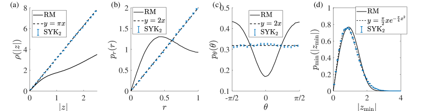
Figure 12: Hard-edge statistics of the two-body non-Hermitian SYK model $H_{\rm SYK}^{q=2}$ in Eq. (58). (a) Density $\rho(|z|)$ of the modulus of eigenvalues. (b) Radial distributions $p_{r}(r)$ and (c) angular distributions $p_{\theta}(\theta)$ of the complex level ratios $re^{\text{i}\theta}$ [Eq. (11)] around the spectral origin. (d) Radial distribution of the eigenvalue $z_{\min}$ with the smallest modulus. The points with the error bars refer to the non-Hermitian SYK model with $q=2$, and the solid curves are obtained by non-Hermitian random matrices (RM) in class D.

VI Open quantum systems beyond the AZ₀ and AZ^† classification

In this section, we study the hard-edge statistics of open quantum systems beyond the AZ₀ classification. Specifically, we focus on the distributions of the complex eigenvalue $z_{\rm min}$ closest to the spectral origin in the three representative symmetry classes, i.e., classes BDI, CI, and AII + $\mathcal{S}_{+}$. We show that the numerically obtained distributions of the physical models match well with the distributions of non-Hermitian random matrices in the corresponding symmetry classes. Notably, in classes BDI and CI, the distributions of $z_{\min}$ show delta-function peaks on the real and imaginary axes, consistent with the random-matrix behavior.

VI.1 Non-interacting systems

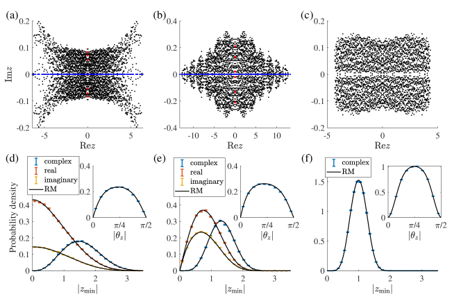
Figure 13: (a)-(c) Complex eigenvalues of single realizations of the non-Hermitian Hamiltonians in Eqs. (64)-(68). Complex, real, and purely imaginary eigenvalues are denoted by the black, blue, and red points, respectively. (d)-(f) Distributions of the complex eigenvalue $z_{\min}$ with the smallest modulus. The blue, orange, and yellow points with the error bars represent the radial distributions of $z_{\min}$ when it is complex, real, and purely imaginary, respectively. Inset: angular distribution of complex $z_{\min}$. The solid curves correspond to non-Hermitian random matrices (RM). (a), (d) Effective non-Hermitian Hamiltonian in Eq. (64) for class BDI. (b), (e) Hamiltonian in Eq. (68) of the non-Hermitian superconductor for class CI. (c), (f) Effective non-Hermitian Hamiltonian in Eq. (65) for class AII + $\mathcal{S}_{+}$.

We introduce three non-interacting models in classes BDI, CI, and AII + $\mathcal{S}_{+}$, respectively. For class BDI, we add the following dissipators

$$L_{{\bm{i}}}=\sqrt{{\gamma}}(c_{{\bm{i}}}+\text{i}c_{{\bm{i}}+2{\bm{e}}_{z}})\quad\left({\bm{i}}\in\mathbb{Z}^{3}\right),$$ (62)

to the random-hopping model $H_{\rm BDI}$ [i.e., Eq. (39) with $t_{{\bm{i}},{\bm{j}}}\in\mathbb{R}$]. For class AII + $\mathcal{S}_{+}$, we add the following dissipators

$$L_{{\bm{i}}\sigma}=\sqrt{{\gamma}}(\psi_{{\bm{i}}\sigma}+\psi_{({\bm{i}}+\text{i}{\bm{e}}_{z})\sigma})\quad\left({\bm{i}}\in\mathbb{Z}^{3},\sigma=\uparrow,\downarrow\right)$$ (63)

to the SU(2) model $H_{\rm CII}$ [i.e., Eq. (39) with $t_{{\bm{i}},{\bm{j}}}\in\rm SU(2)$]. The effective non-Hermitian Hamiltonians of these quadratic Lindbladians in Eq. (38) are given as

$$h_{\rm eff}^{\rm BDI} =H_{\rm BDI}+\gamma\sum_{{\bm{i}}}\left(-c_{{\bm{i}}+2{\bm{e}}_{z}}^{\dagger}c_{{\bm{i}}}+c_{{\bm{i}}}^{\dagger}c_{{\bm{i}}+2{\bm{e}}_{z}}\right)\,,$$ (64)

$$h_{\rm eff}^{{\rm AII}+\mathcal{S}_{+}} =H_{\rm CII}+\gamma\sum_{{\bm{i}}}\left(-c_{{\bm{i}}+{\bm{e}}_{z}}^{\dagger}c_{{\bm{i}}}+c_{{\bm{i}}}^{\dagger}c_{{\bm{i}}+{\bm{e}}_{z}}\right)\,,$$ (65)

respectively. The Hamiltonian $h_{\rm eff}^{\rm BDI}$ satisfies

$$(h_{\rm eff}^{\rm BDI})^{*}=h_{\rm eff}^{\rm BDI},\quad\mathcal{S}(h_{\rm eff}^{\rm BDI})^{\dagger}\mathcal{S}^{-1}=-h_{\rm eff}^{\rm BDI}$$ (66)

with $\mathcal{S}=\delta_{{\bm{i}},{\bm{j}}}(-1)^{({\bm{i}}_{x}+{\bm{i}}_{y}+{\bm{i}}_{z})}$ and hence belongs to class BDI. On the other hand, the Hamiltonian $h_{\rm eff}^{{\rm AII}+\mathcal{S}_{+}}$ satisfies

$$\sigma_{y}(h_{\rm eff}^{{\rm AII}+\mathcal{S}_{+}})^{*}\sigma_{y}=h_{\rm eff}^{{\rm AII}},\quad\mathcal{S}(h_{\rm eff}^{{\rm AII}+\mathcal{S}_{+}})^{{\dagger}}\mathcal{S}^{-1}=-h_{\rm eff}^{{\rm AII}+\mathcal{S}_{+}},$$ (67)

and hence belongs to class AII + $\mathcal{S}_{+}$.

As a non-Hermitian model in class CI, we investigate a three-dimensional non-Hermitian superconductor similar to Eq. (V.3) but with a different form of imbalanced pairing potentials. In the Nambu basis, the Hamiltonian $H_{\rm CI}$ reads

$$H_{\rm CI} =\sum_{{\bm{i}}}\left\{\Psi_{{\bm{i}}}^{\dagger}\left[(\epsilon_{{\bm{i}}}-\mu)\tau_{z}+\text{i}\Delta^{s}_{{\bm{i}}}\tau_{x}\right]\Psi_{{\bm{i}}}\right.$$

$$\left.+\sum_{\mu=x,y,z}\left[\Psi_{{\bm{i}}+{\bm{e}}_{\mu}}^{\dagger}\left(t\tau_{z}+\Delta_{\mu}\tau_{y}\right)\Psi_{{\bm{i}}}+{\rm H.c.}\right]\right\}\,,$$ (68)

where the random chemical potential $\epsilon_{{\bm{i}}}$ is distributed uniformly in $[-W_{1}/2,W_{1}/2]$, and the random imbalanced paring potential $\Delta^{s}_{{\bm{i}}}$ is distributed uniformly in $[-W_{2}/2,W_{2}/2]$. This Hamiltonian $H_{\rm CI}$ satisfies

$$\tau_{z}H_{\rm CI}^{*}\tau_{z}=H_{\rm CI},\quad\tau_{x}H_{\rm CI}^{\dagger}\tau_{x}=-H_{\rm CI}$$ (69)

and hence belongs to class CI.

For each symmetry class, we numerically diagonalize $2\times 10^{5}$ samples of Hamiltonians with the following parameters: (i) Class BDI ($h_{\rm eff}^{\rm BDI}$).—$t=1,W=1.6,\gamma=0.15$, and $L=16$; (ii) Class CI ($H_{\rm CI}$).—$t=2,\mu=0,\Delta_{x}=\Delta_{y}=1,\Delta_{z}=1/2$, $W_{1}=6,W_{2}=3$, and $L=12$; (iii) Class AII + $\mathcal{S}_{+}$ ($h_{\rm eff}^{{\rm AII}+\mathcal{S}_{+}}$).—$\gamma=0.4$ and $L=12$. For the models in classes BDI and CI, a subextensive number of eigenvalues are real or purely imaginary [Figs. 13 (a) and (b)]. The probability of $z_{\min}$ being real or purely imaginary coincides with that of non-Hermitian random matrices in the same symmetry classes (see Table 5). For the model in class AII + $\mathcal{S}_{+}$, by contrast, all eigenvalues are complex, also consistent with the random-matrix behavior [Fig. 13 (c)]. Furthermore, the distributions of $z_{\min}$, including the radial distributions of real, purely imaginary, and complex $z_{\min}$, and the angular distributions of complex $z_{\min}$, in all these models are well described by non-Hermitian random matrices [Figs. 13 (d)-(f)]. In Table 5, we compare $\langle|z_{\min}|\rangle$ from non-Hermitian random matrices and that from the non-Hermitian Hamiltonians. The values are consistent among different systems in the same symmetry class.

Table 5: Mean value $\langle|z_{\min}|\rangle$ and probability of $z_{\min}$ being real or purely imaginary for non-Hermitian random matrices, the Hamiltonians in Eqs. (64)-(68), and the SYK Lindbladians. Here, $z_{\min}$ denotes the complex eigenvalue with the smallest modulus.

Symmetry class and systems	$\langle|z_{\rm min}|^{2}\rangle$	Pr($z_{\min}\in\mathbb{R}$)	Pr($\text{i}z_{\min}\in\mathbb{R}$)
Class BDI
Random matrices	$1.4488(6)$	$0.5373(2)$	$0.1960(2)$
Hamiltonian [Eq. (64)]	$1.447(4)$	$0.536(2)$	$0.196(1)$
SYK Lindbladian	$1.448(6)$	$0.537(2)$	$0.198(2)$
Class CI
Random matrices	$1.2223(4)$	$0.4247(2)$	$0.2732(2)$
Hamiltonian [Eq. (68)]	$1.223(3)$	$0.424(2)$	$0.277(2)$
SYK Lindbladian	$1.226(4)$	$0.425(2)$	$0.272(2)$
Class AII + $\mathcal{S}_{+}$
Random matrices	$1.0623(2)$	$0$	$0$
Hamiltonian [Eq. (65)]	$1.062(2)$	$0$	$0$

VI.2 Many-body Lindbladians

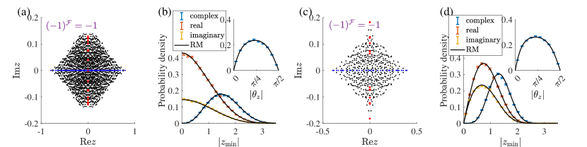
Figure 14: Complex eigenvalues in the symmetry sector $(-1)^{\mathcal{F}}=-1$ of single realizations of the many-body Lindbladians in (a) class BDI ($N=12$) and (b) class CI ($N=10$). Complex, real, and purely imaginary eigenvalues are denoted by the black, blue, and red points, respectively. The distributions of the complex eigenvalue $z_{\min}$ with the smallest modulus for the many-body Lindbladians in (b) class BDI and (d) class CI. The blue, orange, and yellow points with the error bars represent the radial distributions of $z_{\min}$ when it is complex, real, and purely imaginary, respectively. Inset: angular distribution of complex $z_{\min}$. The solid curves correspond to non-Hermitian random matrices (RM).

As a prototypical physical model with strongly correlated fermions coupled to the environment, we study the Lindbladian $\mathcal{L}$ for the SYK model [150, 151, 97]. The Hamiltonian is given by the original SYK model consisting of the $q$-body random interactions,

$$H=\text{i}^{\frac{q}{2}}\sum_{1\leq i_{1}<\cdots<i_{q}\leq N}J_{i_{1}i_{2}\cdots i_{q}}\gamma_{i_{1}}\cdots\gamma_{i_{q}}\,,$$ (70)

where $\gamma_{i}$’s are Majorana operators, $N$ is the number of Majorana fermions, and $J_{i_{1}i_{2}\cdots i_{q}}$’s are independent real Gaussian variables with zero means and $\langle J_{i_{1}i_{2}\cdots i_{q}}^{2}\rangle=((q-1)!/N^{q})\,J^{2}$. Then, we add the following linear dissipators $L_{m}$,

$$L_{m}=\sum_{1\leq i\leq N}K_{m;i}\gamma_{i}\quad(m=1,2,\cdots,M),$$ (71)

where $K_{m;i}$’s are independent complex Gaussian variables with zero means and $\left\langle|K_{m;i}|^{2}\right\rangle=((q-1)!/N^{q})\,K^{2}$.

As discussed in Sec. V.1, after the vectorization of the density matrix, the Lindbladian $\mathcal{L}$ becomes a non-Hermitian operator in the double Hilbert space. It can be represented with the basis of adjoint fermions [84] (see also Appendix D for details), facilitating analytic analyses. The SYK Lindbladian $\mathcal{L}$ respects a unitary symmetry

$$\left(-1\right)^{\mathcal{F}}\mathcal{L}\left(-1\right)^{\mathcal{F}}=\mathcal{L},$$ (72)

where $(-1)^{\mathcal{F}}$ is the total fermion parity operator in the double Hilbert space. For $q=6$, the traceless Lindbladian $\mathcal{L}-{\rm Tr}\mathcal{L}/{\rm Tr}1$ belongs to symmetry class BDI for $N\in 4\mathbb{Z}$ and class CI for $N\in 4\mathbb{Z}+2$ in each sector of total fermion parity $(-1)^{\mathcal{F}}=\pm 1$ (see Ref. [97] and Appendix D for derivations).

We numerically diagonalize $10^{5}$ realizations of the traceless Lindbladians with the following two sets of parameters: (i) Class BDI.—$N=M=12$, $J=1$, and $K=0.4$; (ii) Class CI.—$N=M=10$, $J=1$, and $K=0.3$. The SYK Lindbladians exhibit distinct distributions of $z_{\min}$ for different $N$ [Figs. 14 (b), (d)], consistent with non-Hermitian random matrices in the corresponding symmetry classes (see Table 5).

VII Conclusions and Discussions

In 28 out of 38 symmetry classes of non-Hermitian random matrices, we find that the spectral origin in the complex plane respects higher symmetry compared to other points. We comprehensively investigate the hard-edge statistics in these 28 symmetry classes. This work, combined with the prior works on the threefold universal statistics in the bulk [77] and the sevenfold universal statistics on the real axis [111], forms a foundational comprehension of non-Hermitian random matrix theory across all the 38 symmetry classes. In the seven symmetry classes of the AZ₀ classification, we introduce complex level ratios around the spectral origin and analyze the universality classes of the hard-edge statistics. We numerically obtain the seven universal ratio distributions, with both radial and angular components exhibiting the characteristic behavior. In 21 symmetry classes beyond the AZ₀ classification, we utilize the distributions of complex eigenvalues $z_{\min}$ with the smallest modulus to characterize the hard-edge statistics. In certain symmetry classes, $z_{\min}$ can be real or purely imaginary with the universal probability. This probability serves as practically useful indicators for determining universality classes. Additionally, we perform analytic calculations for small random matrices and elucidate the essential features of our numerical results.

The results of this paper also serve as a diagnostic tool of non-integrability or its absence in open quantum systems with symmetry, as well as the transitions between them. We investigate diverse physical models in the seven AZ₀ symmetry classes and the three representative symmetry classes beyond the AZ₀ classification. In contrast to dense random matrices in the Gaussian ensembles, ensembles of physical Hamiltonians or Lindbladians are regarded as ensembles of sparse matrices because of the locality constraint. It is also noteworthy that symmetry of ensembles of the physical Hamiltonians is generally lower than symmetry of the Gaussian random-matrix ensembles. Nevertheless, the random-matrix hard-edge statistics emerge in both physical Hamiltonians and Lindbladians, showcasing their universality. A direct consequence of this consistency is the emergent spectral U(1) or D₄ symmetry of the ensemble-average distributions of the complex eigenvalues around the spectral origin. To our best knowledge, such emergent spectral symmetry is intrinsic to non-Hermitian systems and has no counterparts in Hermitian random matrix theory.

It is interesting to explore alternative characterizations of hard-edge statistics and their applicability to physical systems. For example, in Appendix C, for non-Hermitian random matrices in classes BDI, CI, and AII + $\mathcal{S}_{+}$, we consider the distributions of complex, real, and purely imaginary eigenvalues, separately. Despite slower convergence with respect to the matrix size, these distributions also appear to be universal and align with physical Hamiltonians. Other potential characterizations, including the spectral compressibility and $n$-point correlation functions [152], are also left for future study.

The symmetry classification of open quantum systems is not limited to Hamiltonians or Lindbladians but also applies to dynamical generators of the non-Markovian dynamics [153]. Investigating and comparing their hard-edge statistics with our results can provide insights into these less-explored, but physically relevant, open quantum systems. The applications of non-Hermitian random matrix theory in classical systems, including complex networks with symmetry, also merit future studies.

Appendix A Form of non-Hermitian random matrices in each symmetry class

We provide explicit forms of non-Hermitian random matrices in chiral and BdG symmetry classes in the AZ₀ classification, whose spectral statistics are investigated in Sec. III. Below, $\tau_{\mu}$ and $\sigma_{\mu}$ $(\mu=0,x,y,z)$ represent Pauli matrices. A generic non-Hermitian random matrix $H$ in class D with $\mathcal{C}_{-}=\sigma_{0}$ is an anti-symmetric complex matrix, satisfying

$$H=-H^{\rm T}\,.$$ (73)

A generic non-Hermitian random matrix $H$ in class C with $\mathcal{C}_{-}=\sigma_{y}$ is given as

$$H=\begin{pmatrix}A&B\\ C&-A^{\rm T}\\ \end{pmatrix}\text{ with }B=B^{\rm T},\,C=C^{\rm T}\,.$$ (74)

A generic non-Hermitian random matrix $H$ in class DIII₀ is given as

$$H=\begin{pmatrix}0&A\\ B&0\end{pmatrix}\text{ with }A=A^{\rm T},\,B=-B^{\rm T}\,,$$ (75)

where the symmetry operators are chosen as $\mathcal{S}=\sigma_{z}$ and $\mathcal{T}_{+}=\sigma_{y}$. A generic non-Hermitian random matrix $H$ in class CI₀ is given as

$$H=\begin{pmatrix}0&A\\ B&0\end{pmatrix}\text{ with }A=A^{\rm T},\,B=B^{\rm T}\,,$$ (76)

with the symmetry operators $\mathcal{S}=\sigma_{z}$ and $\mathcal{T}_{+}=\sigma_{x}$. A generic non-Hermitian random matrix $H$ in class AIII^† is given as

$$H=\begin{pmatrix}0&A\\ B&0\end{pmatrix}\,,$$ (77)

with $\mathcal{S}=\sigma_{z}$. A generic non-Hermitian random matrix $H$ in class BDI₀ is given as

$$H=\begin{pmatrix}0&A\\ A^{\rm T}&0\end{pmatrix}\,,$$ (78)

with $\mathcal{S}=\sigma_{z}$ and $\mathcal{T}_{+}=\sigma_{0}$. A generic non-Hermitian random matrix $H$ in class CII₀ is given as

$$H=\begin{pmatrix}0&0&A&B\\ 0&0&C&D\\ D^{\rm T}&-B^{\rm T}&0&0\\ -C^{\rm T}&A^{\rm T}&0&0&\end{pmatrix}\text{ with }A_{ij},B_{ij},C_{ij},D_{ij}\in\mathbb{C}\,,$$ (79)

where the symmetry operators are chosen as $\mathcal{S}=\tau_{z}\otimes\sigma_{0}$ and $\mathcal{T}_{+}=\tau_{0}\otimes\sigma_{y}$.

Additionally, we give explicit forms of non-Hermitian random matrices in classes BDI, CI, and AII + $\mathcal{S}_{+}$, whose spectral statistics are investigated in Sec. IV. A generic random matrix $H$ in class BDI is given as

$$H=\begin{pmatrix}A&B\\ B^{\rm T}&C\\ \end{pmatrix}\, \text{with }A=-A^{\rm T},\,C=-C^{\rm T},$$

$$\quad\text{and }A_{ij},B_{ij},C_{ij}\in\mathbb{R}\,,$$ (80)

where the symmetry operators are chosen as $\mathcal{T}_{+}=\tau_{0}$ and $\mathcal{C}_{-}=\tau_{z}$. A generic non-Hermitian random matrix $H$ in class CI is given as

$$H=\begin{pmatrix}A&B\\ C&-A^{\rm T}\\ \end{pmatrix}\, \text{with }B=B^{\rm T},\,C=C^{\rm T},\,$$

$$\text{and }A_{ij},B_{ij},C_{ij}\in\mathbb{R}\,,$$ (81)

with $\mathcal{T}_{+}=\tau_{0}$ and $\mathcal{C}_{-}=\tau_{y}$. A generic non-Hermitian random matrix $H$ in class AII + $\mathcal{S}_{+}$ is given as

$$H=\begin{pmatrix}0&0&A&B\\ 0&0&-B^{*}&A^{*}\\ C&D&0&0\\ -D^{*}&C^{*}&0&0&\end{pmatrix}\text{ with }A_{ij},B_{ij},C_{ij},D_{ij}\in\mathbb{C}\,,$$ (82)

with $\mathcal{T}_{+}=\tau_{0}\otimes\sigma_{y}$ and $\mathcal{S}=\tau_{z}\otimes\sigma_{0}$.

Appendix B Analytic results

B.1 Level-ratio distributions around the spectral origin

B.1.1 Class AIII^†

We consider $4\times 4$ non-Hermitian random matrices in the Gaussian ensemble in class AIII^†. Let $\pm z_{1},\pm z_{2}$ be its eigenvalues. We also introduce $y_{i}\equiv z_{i}^{2}$ ($i=1,2$). The joint probability density function $\rho(y_{1},y_{2})$ of $y_{1},y_{2}$ is given as [19]

$$\rho(y_{1},y_{2})\propto K_{0}(|y_{1}|)K_{0}(|y_{2}|)|y_{1}-y_{2}|^{2}\,,$$ (83)

where $K_{0}(\cdot)$ is the modified Bessel function of the second kind. With $y_{i}\equiv|y_{i}|e^{\text{i}\phi_{i}}$, the probability density function for $|y_{i}|,\phi_{i}$ is given as

$$\rho(|y_{1}|,\phi_{1},|y_{2}|,\phi_{2})\propto K_{0}(|y_{1}|)K_{0}(|y_{2}|)|y_{1}||y_{2}|$$

$$\qquad\quad\times\left[|y_{1}|^{2}+|y_{2}|^{2}-2|y_{1}||y_{2}|\cos(\phi_{1}-\phi_{2})\right]\,.$$ (84)

Integrating $\rho(|y_{1}|,\phi_{1},|y_{2}|,\phi_{2})$ over $\phi_{1},\phi_{2}$, we have

$$\rho(|y_{1}|,|y_{2}|)\propto K_{0}(|y_{1}|)K_{0}(|y_{2}|)|y_{1}||y_{2}|\left(|y_{1}|^{2}+|y_{2}|^{2}\right)\,.$$ (85)

Let us introduce $|y_{2}|=R|y_{1}|$. Using $d|y_{1}|d|y_{2}|=|y_{1}|d|y_{1}|dR$, we further have

$$\rho(|y_{1}|,R)\propto K_{0}(|y_{1}|)K_{0}(R|y_{1}|)|y_{1}|^{5}R\left(1+R^{2}\right)\,.$$ (86)

We then integrate $\rho(|y_{1}|,R)$ over $|y_{1}|$, leading to

$$\rho(R)=\frac{4R\left(R^{2}+1\right)\left(-3R^{4}+2\left(R^{4}+4R^{2}+1\right)\ln R+3\right)}{\left(R^{2}-1\right)^{5}}\,.$$ (87)

The distribution function of the level ratio $r\equiv|z_{1}/z_{2}|=\sqrt{R}$ is given as

$$p_{r}^{N=4}(r)$$

$$= \frac{16r^{3}\left(r^{4}+1\right)\left(-3r^{8}+4\left(r^{8}+4r^{4}+1\right)\ln r+3\right)}{\left(r^{4}-1\right)^{5}}\,.$$ (88)

Here, an extra factor of two is due to the assumption $|z_{1}|\leq|z_{2}|$. For $r\ll 1$, we have $\rho_{r}(r)\propto-r^{3}\ln r$, which is consistent with the numerical results from large random matrices (see Table 2).

We can also integrate $\rho(|y_{1}|,\phi_{1},|y_{2}|,\phi_{2})$ in Eq. (84) over $|y_{1}|,|y_{2}|$, leading to

$$\rho(\phi_{1},\phi_{2})\propto 8-\frac{\pi^{2}}{2}\cos(\phi_{1}-\phi_{2})\,.$$ (89)

Since the phase $\theta$ of the level ratio $z_{1}/z_{2}$ equals $(\phi_{1}-\phi_{2})/2$, its distribution function is obtained as

$$p_{\theta}^{N=4}=\frac{16-\pi^{2}\cos 2\theta}{16\pi}\,.$$ (90)

The angular distribution $p_{\theta}^{N=4}$ reaches its maximum and minimum at $\theta=\pm\pi/2$ and $\theta=0$, respectively, consistent with the numerical results of large random matrices [see Fig. 9 (c)].

B.1.2 Class D

A $4\times 4$ non-Hermitian random matrix $H$ in class D, satisfying $H=-H^{\rm T}$, can be given as

$$H=\sum_{\mu=0,x,z}\left(a_{\mu}\tau_{\mu}\sigma_{y}+b_{\mu}\tau_{y}\sigma_{\mu}\right)\quad$$ (91)

with $a_{\mu},b_{\mu}\in\mathbb{C}$. In the Gaussian ensemble with the probability density $p(H)\propto e^{-\beta\,{\rm Tr}\,(H^{\dagger}H)}$, $a_{\mu}$ and $b_{\mu}$ are independent complex Gaussian variables with zero means. The four eigenvalues of $H$ are

$$\pm z_{1}=\pm\left(w_{1}-w_{2}\right),\quad\pm z_{2}=\pm\left(w_{1}+w_{2}\right)$$ (92)

with

$$w_{1}\equiv\sqrt{b_{0}^{2}+a_{x}^{2}+a_{z}^{2}},\quad w_{2}\equiv\sqrt{a_{0}^{2}+b_{x}^{2}+b_{z}^{2}}\,.$$ (93)

Notably, $w_{1}$ and $w_{2}$ are independent complex random variables with the identical probability distribution in the complex plane [77],

$$\rho(w)=\frac{1}{\pi}|w|^{2}e^{-|w|^{2}}\,.$$ (94)

The radial distribution of $w$ is given as

$$p_{w}(|w|=s) =\int\rho(w)\delta(|w|-s)dwdw^{*}$$

$$=2|s|^{3}e^{-|s|^{2}}\,.$$ (95)

The radial distribution of $t\equiv w_{1}/w_{2}$ is given as

$$p_{t}(|t|=x) =\int p_{w}(|w|=s_{1})p_{w}(|w|=s_{2})$$

$$\qquad\qquad\qquad\times\delta(s_{1}/s_{2}-x)ds_{1}ds_{2}$$

$$=\frac{12x^{3}}{(1+x^{2})^{4}}\,.$$ (96)

Thus, the probability density of $t$ in the complex plane is

$$\rho(t)=\frac{6|t|^{2}}{\pi(1+|t|^{2})^{4}}\,.$$ (97)

The complex level ratio $v\equiv re^{\text{i}\theta}\equiv z_{1}/z_{2}=(1+t)/(1-t)$ is a meromorphic function of $t$. Then, the probability density of $v$ in the complex plane is given as

$$\rho(v) =\frac{6|t|^{2}}{\pi(1+|t|^{2})^{4}}\left\lvert\frac{dt}{dv}\right\rvert^{2}$$

$$=\frac{24}{\pi}\frac{\left(1+r^{2}+2r\cos\theta\right)\left(1+r^{2}-2r\cos\theta\right)}{\left(2+2r^{2}\right)^{4}}\,.$$ (98)

Integrating $\rho(v)$ over $\theta$ or $r$, we obtain the radial and angular distributions of the complex level ratio $v$ as

$$p_{r}^{N=4}(r) =\frac{6(1+r^{4})r}{(1+r^{2})^{4}}\,,$$ (99)

$$p_{\theta}^{N=4}(\theta) =\frac{2-\cos 2\theta}{4\pi}\,,$$ (100)

respectively. For $r\ll 1$, we have $p_{r}^{N=4}(r)\propto r$, and $p_{\theta}^{N=4}$ reaches its maximum and minimum at $\theta=\pm\pi/2$ and $\theta=0$, respectively, consistent with numerical results from large random matrices [see Table 2 and Fig. 9 (c)].

B.2 Density of complex eigenvalues

B.2.1 Classes D and BDI₀

A generic $2\times 2$ non-Hermitian matrix $H$ in class D, which respects PHS $H^{\rm T}=-H$, is given as

$$H=a_{y}\sigma_{y}\quad\left(a_{y}\in\mathbb{C}\right).$$ (101)

The two complex eigenvalues of $H$ are obtained as $\pm z=\pm a_{y}$. Notably, $\left|z\right|=\left|a_{y}\right|$ is essentially equivalent to the level spacing between the two eigenvalues of $2\times 2$ Hermitian matrices in class AI. Consequently, the probability distribution function $\rho\left(\left|z\right|\right)$ is the same as the level-spacing distribution for $2\times 2$ Hermitian random matrices in class AI.

Suppose that $H$ obeys the Gaussian probability distribution $\propto e^{-\beta\,\mathrm{Tr}\,(H^{{\dagger}}H)/2}=e^{-\beta\,(y_{\rm r}^{2}+y_{\rm i}^{2})}$ with a constant $\beta>0$ and $y_{\rm r}\equiv\mathrm{Re}\,a_{y}$, $y_{\rm i}\equiv\mathrm{Im}\,a_{y}$. Then, the probability distribution function $\rho\left(\left|z\right|\right)$ reads

$$\rho\left(\left|z\right|\right) =\frac{\beta}{\pi}\int_{-\infty}^{\infty}dy_{\rm r}dy_{\rm i}~{}\delta\left(\left|z\right|-\sqrt{y_{\rm r}^{2}+y_{\rm i}^{2}}\right)e^{-\beta\,(y_{\rm r}^{2}+y_{\rm i}^{2})}.$$ (102)

Introducing the polar coordinate $r\equiv\sqrt{y_{\rm r}^{2}+y_{\rm i}^{2}}$, we have

$$\rho\left(\left|z\right|\right) =2\beta\int_{0}^{\infty}dr~{}r~{}\delta\left(\left|z\right|-r\right)e^{-\beta r^{2}}$$

$$=2\beta\left|z\right|e^{-\beta\left|z\right|^{2}}.$$ (103)

To further impose the normalization condition $\int_{0}^{\infty}\left|z\right|\rho\left(\left|z\right|\right)d\left|z\right|=1$, we should choose $\beta$ as $\beta=\pi/4$. Notably, $\rho\left(\left|z\right|\right)$ linearly vanishes at the spectral origin,

$$\rho\left(\left|z\right|\right)\simeq 2\beta\left|z\right|$$ (104)

for small $\left|z\right|\ll 1$. This linear decay of $\rho\left(\left|z\right|\right)$ does not necessarily mean the level repulsion around the origin since it just arises from the two-dimensional integral measure along the angle direction. A similar result was obtained in Ref. [93].

A generic $2\times 2$ non-Hermitian matrix $H$ in class BDI₀ (or equivalently, class D + $\mathcal{S}_{+}$), which respects SLS $\sigma_{z}H\sigma_{z}=-H$ and PHS $H^{\rm T}=-H$, is again given as Eq. (101). Consequently, the probability distribution function $\rho\left(\left|z\right|\right)$ is the same as $\rho\left(\left|z\right|\right)$ in class D [i.e., Eq. (103)]. However, this is specific to small non-Hermitian matrices. For larger non-Hermitian matrices, $\rho\left(\left|z\right|\right)$’s are different between classes D and BDI owing to the many-level effect, as shown in Fig. 3.

B.2.2 Class C

A generic $2\times 2$ non-Hermitian matrix $H$ in class C, which respects PHS $\tau_{y}H^{\rm T}\tau_{y}=-H$, is given as

$$H=a_{x}\tau_{x}+a_{y}\tau_{y}+a_{z}\tau_{z}\quad\left(a_{x},a_{y},a_{z}\in\mathbb{C}\right).$$ (105)

The probability distribution function $\rho\left(\left|z\right|\right)$ of $\left|z\right|=\left|\sqrt{a_{x}^{2}+a_{y}^{2}+a_{z}^{2}}\right|$ is equivalent to the level-spacing distribution of $2\times 2$ non-Hermitian random matrices in class A, which is analytically obtained as [77]

$$\rho\left(\left|z\right|\right)=2C_{3}^{4}\left|z\right|^{3}e^{-C_{3}^{2}\left|z\right|^{2}}$$ (106)

with the normalization constant $C_{3}\equiv 3\sqrt{\pi}/4=1.32934\cdots$. Here, $\rho\left(\left|z\right|\right)$ is normalized by $\int_{0}^{\infty}\rho\left(\left|z\right|\right)d\left|z\right|=\int_{0}^{\infty}\left|z\right|\rho\left(\left|z\right|\right)d\left|z\right|=1$. For small $\left|z\right|\ll 1$, we have

$$\rho\left(\left|z\right|\right)\simeq 2C_{3}^{4}\left|z\right|^{3}.$$ (107)

The cubic decay of $\rho\left(\left|z\right|\right)$ means the level repulsion around the origin. A similar result was obtained in Ref. [93].

B.2.3 Class CII₀

No generic $2\times 2$ non-Hermitian matrix $H$ is present in class CII₀ (or equivalently, class C + $\mathcal{S}_{+}$). A generic $4\times 4$ non-Hermitian matrix $H$ in class CII₀, which respects TRS^† $\sigma_{y}H^{\rm T}\sigma_{y}=H$ and PHS $\tau_{y}H^{\rm T}\tau_{y}=-H$, is given as

$$H=a_{x}\tau_{x}+\left(b_{x}\sigma_{x}+b_{y}\sigma_{y}+b_{z}\sigma_{z}\right)\tau_{y}+a_{z}\tau_{z}$$ (108)

with $a_{x},a_{z},b_{x},b_{y},b_{z}\in\mathbb{C}$. The eigenvalues are obtained as

$$\pm z=\pm\sqrt{a_{x}^{2}+a_{z}^{2}+b_{x}^{2}+b_{y}^{2}+b_{z}^{2}},$$ (109)

and exhibit the two-fold degeneracy due to TRS^†. Thus, the probability distribution function $\rho\left(\left|z\right|\right)$ is equivalent to the level-spacing distribution of $2\times 2$ non-Hermitian random matrices in class AII^†, which is analytically obtained as [77]

$$\rho\left(\left|z\right|\right)=\frac{2C_{5}^{4}}{3}\left|z\right|^{3}\left(1+C_{5}^{2}\left|z\right|^{2}\right)e^{-C_{5}^{2}\left|z\right|^{2}}$$ (110)

with the normalization constant $C_{5}\equiv 7\sqrt{\pi}/8=1.5509\cdots$. Here, $\rho\left(\left|z\right|\right)$ is normalized by $\int_{0}^{\infty}\rho\left(\left|z\right|\right)d\left|z\right|=\int_{0}^{\infty}\left|z\right|\rho\left(\left|z\right|\right)d\left|z\right|=1$. For small $\left|z\right|\ll 1$, we have

$$\rho\left(\left|z\right|\right)\simeq\frac{2C_{5}^{4}}{3}\left|z\right|^{3}.$$ (111)

The cubic decay of $\rho\left(\left|z\right|\right)$ means the level repulsion around the origin.

B.2.4 Classes AIII^†, DIII₀, and CI₀

A generic $2\times 2$ non-Hermitian matrix $H$ in class AIII^†, which respects SLS $\sigma_{z}H\sigma_{z}=-H$, is given as

$$H=a_{x}\sigma_{x}+a_{y}\sigma_{y}\quad\left(a_{x},a_{y}\in\mathbb{C}\right).$$ (112)

The two eigenvalues of $H$ are obtained as

$$\pm z=\pm\sqrt{a_{x}^{2}+a_{y}^{2}}.$$ (113)

Notably, the density of complex eigenvalues, $\rho\left(\left|z\right|\right)$, is equivalent to the level-spacing statistics of $2\times 2$ non-Hermitian matrices in class AI^†, which are analytically obtained as [77]

$$\rho\left(\left|z\right|\right)=2C_{2}^{4}\left|z\right|^{3}K_{0}\,(C_{2}^{2}\left|z\right|^{2}),$$ (114)

where $C_{2}\equiv\left[\Gamma\left(1/4\right)\right]^{2}/8\sqrt{2}=1.16187\cdots$ is a normalization constant, and $K_{0}$ is the modified Bessel function of the second kind. Here, $\rho\left(\left|z\right|\right)$ is normalized by $\int_{0}^{\infty}\rho\left(\left|z\right|\right)d\left|z\right|=\int_{0}^{\infty}\left|z\right|\rho\left(\left|z\right|\right)d\left|z\right|=1$. For small $\left|z\right|\ll 1$, we have $K_{0}\,(C_{2}^{2}\left|z\right|^{2})\simeq-\ln\,(C_{2}^{2}\left|z\right|^{2})$ and hence

$$\rho\left(\left|z\right|\right)\simeq-4C_{2}^{4}\left|z\right|^{3}\ln\left(C_{2}\left|z\right|\right).$$ (115)

A similar result was obtained in Refs. [112, 93]. In the previous analyses [77, 111], the logarithmic correction arises only in the presence of TRS^† with the positive sign $+1$. By contrast, the logarithmic correction appears in the hard-edge statistics with SLS, even in the absence of TRS^†.

No generic $2\times 2$ non-Hermitian matrix $H$ is present in class DIII₀ (or equivalently, class D + $\mathcal{S}_{-}$). A generic $4\times 4$ non-Hermitian matrix $H$ in class DIII₀, which respects TRS^† $\sigma_{y}H^{\rm T}\sigma_{y}=H$ and SLS $\left(\sigma_{z}\tau_{z}\right)H\left(\sigma_{z}\tau_{z}\right)=-H$, is given as

$$H=a_{x}\tau_{x}+a_{y}\sigma_{z}\tau_{y}\quad\left(a_{x},a_{y}\in\mathbb{C}\right).$$ (116)

The modulus of the two eigenvalues is $\left|z\right|=\left|\sqrt{a_{x}^{2}+a_{y}^{2}}\right|$, and hence the probability distribution function $\rho\left(\left|z\right|\right)$ is equivalent to $\rho\left(\left|z\right|\right)$ in class AIII^† [i.e., Eq. (114)].

A generic $2\times 2$ non-Hermitian matrix $H$ in class CI₀ (or equivalently, class C + $\mathcal{S}_{-}$), which respects PHS $\tau_{y}H^{\rm T}\tau_{y}=-H$ and TRS^† $H^{\rm T}=H$, is given as

$$H=a_{x}\tau_{x}+a_{z}\tau_{z}\quad\left(a_{x},a_{z}\in\mathbb{C}\right).$$ (117)

Hence, the probability distribution function $\rho\left(\left|z\right|\right)$ of $\left|z\right|=\left|\sqrt{a_{x}^{2}+a_{z}^{2}}\right|$ is equivalent to $\rho\left(\left|z\right|\right)$ in class AIII^† [i.e., Eq. (114)].

B.3 Distributions of the eigenvalue with the smallest modulus

B.3.1 Class BDI

The minimal dimension of generic non-Hermitian random matrices in class BDI is four. A $4\times 4$ non-Hermitian random matrix $H$ in class BDI with $\mathcal{T}_{+}=\tau_{z}$ and $\mathcal{C}_{-}=1$ is expressed as Eq. (91) with $a_{x},b_{0},b_{x},b_{z},\text{i}a_{0},\text{i}a_{z}\in\mathbb{R}$. In the Gaussian ensemble, $a_{x},b_{0},b_{x},b_{z},\text{i}a_{0},\text{i}a_{z}$ are independent real Gaussian variables with zero means. The four eigenvalues of $H$ are

$$\pm z_{1}=\pm\left(w_{1}-w_{2}\right),\quad\pm z_{2}=\pm\left(w_{1}+w_{2}\right)$$ (118)

with

$$w_{1}\equiv\sqrt{b_{0}^{2}+a_{x}^{2}+a_{z}^{2}},\quad w_{2}\equiv\sqrt{a_{0}^{2}+b_{x}^{2}+b_{z}^{2}}\,.$$ (119)

Therefore, $w_{1}$ and $w_{2}$ are independent random variables with the same probability density function. Here, $w_{1}$ and $w_{2}$ are either real or purely imaginary, and we require ${\rm Re}\,w_{1}\geq 0$ and ${\rm Im}\,w_{2}\geq 0$. The probability density $\rho(w_{1}=\alpha+\text{i}\beta)$ of $w_{1}$ in the complex plane is given as [111]

$$\rho(w_{1}=\alpha+\text{i}\beta)=\frac{\alpha e^{-\alpha^{2}/2}}{\sqrt{2}}\delta(\beta)+\frac{\beta e^{\beta^{2}/2}{\rm erfc}(\beta)}{\sqrt{2}}\delta(\alpha)\,.$$ (120)

According to whether $w_{1}$ and $w_{2}$ are real or purely imaginary, we have three possible cases, as follows.

(i) Both $w_{1}$ and $w_{2}$ are real.—In this case, all the four eigenvalues of $H$ are real. Without loss of generality, we can assume $w_{1}\geq w_{2}\geq 0$. Then, we have $z_{2}=w_{1}+w_{2}>z_{1}=w_{1}-w_{2}\geq 0$, and hence $z_{1}$ is the eigenvalue with the smallest modulus. The probability density $p_{\min;r}(x)$ of $z_{1}=x\geq 0$ is given as

$$p_{\rm min;r}^{N=4}(x)=\int_{0}^{\infty}d\alpha~{}\alpha\left(\alpha+x\right)e^{-(\alpha^{2}+(\alpha+x)^{2})/2}$$

$$=\frac{e^{-x^{2}/2}}{8}\left(2x-\sqrt{\pi}e^{x^{2}/4}\left(x^{2}-2\right)\text{erfc}\left(x/2\right)\right)\,,$$ (121)

satisfying $p_{\min;r}(0)=\sqrt{\pi}/4\approx 0.443$.

(ii) Both $w_{1}$ and $w_{2}$ are purely imaginary.—In this case, the four eigenvalues of $H$ are purely imaginary. Without loss of generality, we can assume $|w_{1}|\geq|w_{2}|\geq 0$. The probability density $p_{\min;i}(|z_{1}|)$ of the eigenvalue $z_{1}=\text{i}y$ with the smallest modulus is given as

$$\quad p_{\rm min;i}^{N=4}(y)=\int_{0}^{\infty}d\beta~{}\beta\left(\beta+y\right){\rm erfc}\left(\beta\right){\rm erfc}\left(\beta+y\right),$$ (122)

satisfying $p_{\rm min;i}(|z_{1}|=0)=\left(1-\ln 2\right)/\left(2\sqrt{\pi}\right)\approx 0.087$. For generic $y$, this integral cannot be expressed by elementary functions.

(iii) One of $w_{1}$ and $w_{2}$ is real, and the other is purely imaginary.—In this case, $z_{1}$ and $z_{2}$ are both complex with $|z_{1}|=|z_{2}|$. Without loss of generality, we can assume $w_{1}\in\mathbb{R}$ and $\text{i}w_{2}\in\mathbb{R}$. The probability density $p_{\rm min;c}(z_{2}=x+\text{i}y)$ of $z_{\min}=|z_{\min}|e^{\text{i}\theta_{z}}$ in the complex plane is given as

$$p_{\rm min;c}^{N=4}(x,y)=xye^{(-x^{2}+y^{2})/2}{\rm erfc}\left(y\right).$$ (123)

For $|z_{\rm min}|\ll 1$, we have $p_{\rm min;c}(x,y)\propto|z_{\rm min}|^{2}$. Thus, the radial distribution $p^{(r);N=4}_{\rm min;c}(|z_{\rm min}|)$ of $|z_{\min}|$ is proportional to $|z_{\min}|^{3}$ for $|z_{\min}|\ll 1$. We can also verify that the angular distribution satisfies $p^{(\theta_{z});N=4}_{\rm min;c}(\theta_{z})\propto|\theta_{z}|$ for $|\theta_{z}|\ll 1$ and $p^{(\theta_{z});N=4}_{\rm min;c}(\theta_{z})\propto|\pi/2-\theta_{z}|$ for $|\pi/2-\theta_{z}|\ll 1$. Thus, the distributions of the eigenvalues with the smallest modulus obtained by the $4\times 4$ non-Hermitian random matrix are qualitatively the same as those of large random matrices [see Figs. 6 (a) and (g)].

B.3.2 Class AII + $\mathcal{S}_{+}$

The minimal dimension of generic non-Hermitian random matrices in class AII + $\mathcal{S}_{+}$ is four, whose eigenvalues appear in quartets as $\left(z,-z,z^{*},-z^{*}\right)$ with the same modulus. The probability distribution $\rho(z)$ is analytically obtained as [119]

$$\rho(z)=\frac{1}{128\pi}\left\lvert z^{2}-(z^{*})^{2}\right\rvert^{2}\lvert z\rvert^{2}K_{0}\left(4\lvert z\rvert^{2}\right)\,.$$ (124)

In class AII + $\mathcal{S}_{+}$, the probability of an eigenvalue being real or purely imaginary is zero, leading to

$$p_{\min;c}^{N=4}(z)=p_{\min}^{N=4}(z)=\rho(z).$$ (125)

Thus, the radial distribution $p_{\min;c}^{(r);N=4}(|z_{\min}|)$ of $z_{\min}=|z_{\min}|e^{\text{i}\theta_{z}}$ with $\theta_{z}\in[0,\pi)$ is given as

$$p_{\min;c}^{(r);N=4}(|z_{\min}|)=\frac{1}{32}|z_{\min}|^{7}K_{0}(|z_{\min}|^{2})\,,$$ (126)

and the angular distribution

$$p_{\min;c}^{(\theta_{z});N=4}=\frac{4}{\pi}\cos^{2}2\theta_{z}.$$ (127)

Specifically, we have

$$p_{\min;c}^{(r);N=4}(|z_{\min}|)\propto-|z_{\min}|^{7}\ln|z_{\min}|\quad\left(|z_{\min}|\ll 1\right)$$ (128)

and

$$p^{(\theta_{z});N=4}_{\rm min;c}(\theta_{z})\propto\begin{cases}|\theta_{z}|^{2}&\left(|\theta_{z}|\ll 1\right);\\ |\pi/2-\theta_{z}|^{2}&\left(|\pi/2-\theta_{z}|\ll 1\right).\end{cases}$$ (129)

These behaviors for $N=4$ are both consistent with the behaviors for large $N$ [see Figs. 6 (c) and (g)].

Appendix C Additional characterization of hard-edge statistics

For non-Hermitian random matrices in some symmetry classes beyond the AZ₀ and AZ^† classification (see Table 3), a subextensive number of eigenvalues are real or purely imaginary. We also find that in these symmetry classes, the level correlations of complex eigenvalues are qualitatively different from those of the real or purely imaginary eigenvalues (see Fig. 6). To characterize the level statistics in these symmetry classes, besides studying the eigenvalue $z_{\min}$ with the smallest modulus (see Sec. IV for details), we here study complex, real, and purely imaginary eigenvalues, separately. Let $c_{\min}$, $\mathcal{R}_{\min}$, and $\mathcal{I}_{\min}$ be the complex, real, and purely imaginary eigenvalues with the smallest modulus, respectively. Owing to the defining symmetries, we can require ${\rm Re}\,c_{\min},{\rm Im}\,c_{\min}>0$, $\mathcal{R}_{\min}\geq 0$, and $\mathcal{I}_{\min}\geq 0$ without loss of generality. As in Sec. IV.1, we here focus on the three representative symmetry classes, i.e., classes BDI, CI, and AII + $\mathcal{S}_{+}$.

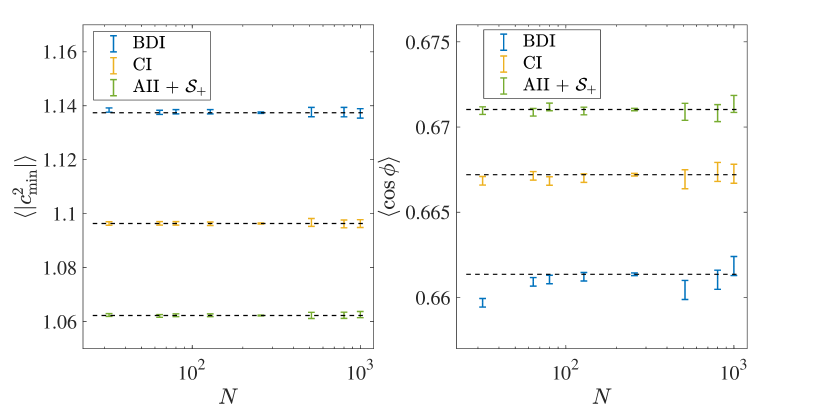
Figure 15: Mean values $\left\langle|c_{\min}|^{2}\right\rangle$ and $\left\langle\cos\phi\right\rangle$ as functions of the matrix size $N$, where $c_{\min}=|c_{\min}|e^{\text{i}\phi}$ is the complex eigenvalue with the smallest modulus. For each symmetry class and each matrix size, $N_{\rm sample}$ samples are diagonalized, with $N_{\rm sample}=10^{7},10^{6},2\times 10^{5}$ for $N=256$, $N<256$, $N>256$, respectively. The dashed lines denote the mean values obtained by matrices with $N=256$.

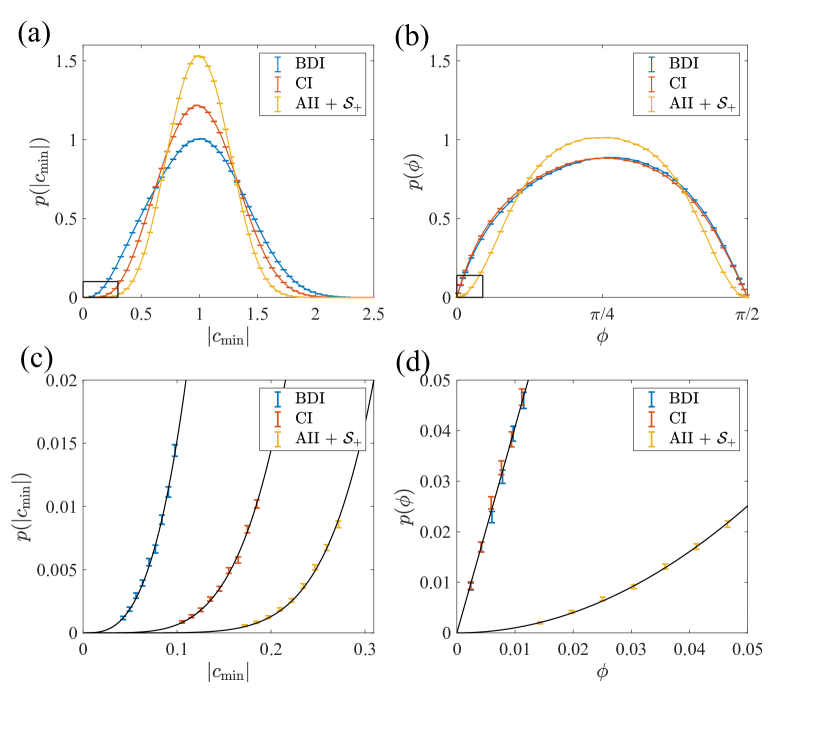
Figure 16: (a) Radial and (b) angular distributions of the complex eigenvalues with the smallest modulus for $256\times 256$ non-Hermitian random matrices in classes BDI, CI, and AII + $\mathcal{S}_{+}$. (c) Zoom-in of subfigure (a) around $\left|c_{\rm min}\right|=0$. The three black curves from left to right are the fitting curves $p(\left|c_{\rm min}\right|)\propto\left|c_{\rm min}\right|^{3}$, $p(\left|c_{\rm min}\right|)\propto-\left|c_{\rm min}\right|^{5}\ln\left|c_{\rm min}\right|$, and $p(\left|c_{\rm min}\right|)\propto-\left|c_{\rm min}\right|^{7}\ln\left|c_{\rm min}\right|$, respectively. (d) Zoom-in of subfigure (b) around $\left|c_{\rm min}\right|=0$. The two black curves from left to right are the fitting curves $p(\left|c_{\rm min}\right|)\propto\left|c_{\rm min}\right|$ and $p(\left|c_{\rm min}\right|)\propto\left|c_{\rm min}\right|^{2}$, respectively.

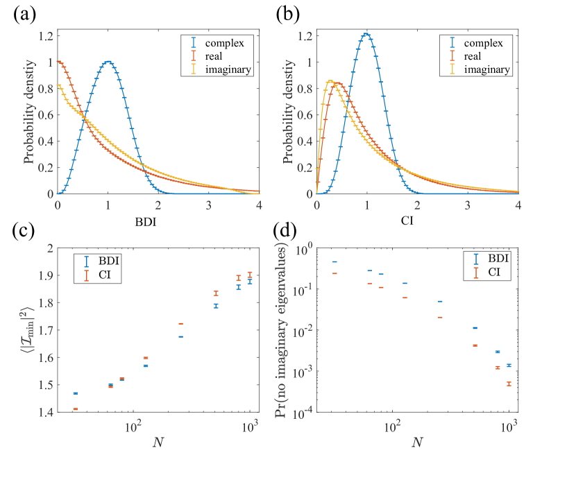
Figure 17: Distributions of the complex, real, and purely imaginary eigenvalues with the smallest modulus for $256\times 256$ non-Hermitian random matrices in (a) class BDI and (b) class CI. For a small proportion $p$ of random matrices, real eigenvalues ($p\approx 0.02\%$) or purely imaginary eigenvalues ($p\approx 3.5\%$) are absent. We exclude such matrices in the statistics of real or imaginary eigenvalues. (c) Mean values $\left\langle\mathcal{I}_{\min}^{2}\right\rangle$ and (d) probability that no purely imaginary eigenvalues exist as functions of the matrix size $N$.

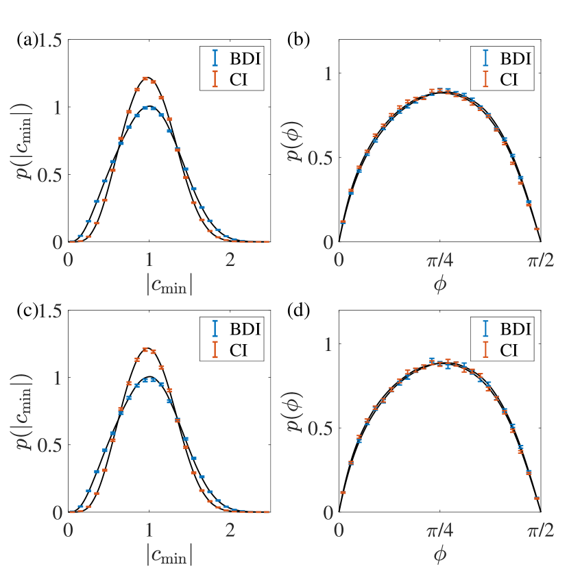
Figure 18: (a), (c) Radial and (b), (d) angular distributions of the complex eigenvalue $c_{\min}$ with the smallest modulus for the non-Hermitian Hamiltonians and many-body Lindbladians. The points with the error bars correspond to the quantum systems, and the solid curves are obtained by the random matrices in the same symmetry classes. (a), (b) Effective non-Hermitian Hamiltonian in Eq. (64) for class BDI and non-Hermitian superconductor in Eq. (68) for class CI. (c), (d) Many-body Lindbladians of the SYK model in Eqs. (70) and (71) for classes BDI ($N=12$) and CI ($N=10$), where we use the eigenvalues in the subsector of $(-1)^{\mathcal{F}}=-1$ to obtain the statistics.

We first investigate the distribution of $c_{\min}=|c_{\min}|e^{\text{i}\phi}$ for non-Hermitian random matrices in classes BDI, CI, and AII + $\mathcal{S}_{+}$. We normalize $c_{\min}$ such that $\left\langle|c_{\rm min}|\right\rangle=1$. In class AII + $\mathcal{S}_{+}$, all eigenvalues are complex, and hence we have $c_{\min}=z_{\min}$. For $N\geq 256$, $\left\langle|c_{\min}|^{2}\right\rangle$ and $\left\langle\cos\phi\right\rangle$ converge to the characteristic values in each symmetry class (see Fig. 15), implying the convergence of the distributions of $z_{\min}$. In each symmetry class, the distribution of $c_{\min}$ is similar to that of complex $z_{\min}$. The radial distributions $p(|c_{\min}|)$ exhibit the characteristic small-$|c_{\min}|$ behavior [see Figs. 16 (a), (c)],

$$p(|c_{\min}|)\propto\begin{cases}|c_{\min}|^{3}&\text{(class BDI)}\,;\\ -|c_{\min}|^{5}\ln|c_{\min}|&\text{(class CI)}\,;\\ -|c_{\min}|^{7}\ln|c_{\min}|&\text{(class AII}+\mathcal{S}_{+})\,.\\ \end{cases}$$ (130)

This is the same as the small-$|z_{\min}|$ behavior of $p_{\rm min;c}(|z_{\min}|)$ in the same symmetry classes (Fig. 6). The angular distributions $p(\phi)$ of $c_{\min}$ are also similar to those of complex $z_{\min}$ [compare Figs. 16 (b), (d) with Fig. 13].

Then, we study the distributions of $\mathcal{R}_{\min}$ and $\mathcal{I}_{\min}$ in classes BDI and CI. In each symmetry class, the distributions $p(\mathcal{R}_{\min})$ and $p(\mathcal{I}_{\min})$ share the same small-$\mathcal{R}_{\min}$ or small-$\mathcal{I}_{\min}$ behavior as $p_{\min:{\rm r}/{\rm i}}(|z_{\min}|)$. However, $p(\mathcal{R}_{\min})$ and $p(\mathcal{I}_{\min})$ are long-tailed in contrast to $p_{\min:{\rm r}/{\rm i}}(|z_{\min}|)$. The statistics of $\mathcal{I}_{\min}$ converge much more slowly than the statistics of $c_{\min}$ and do not converge even for $N=1000$ [see Figs. 17 (c) and (d)]. Thus, $p(|c_{\min}|)$ or $p(\mathcal{R}_{\min})$ should be a more computationally efficient measure of the level statistics than $p(\mathcal{I}_{\min})$.

Furthermore, we compare $p(|c_{\min}|)$ and $p(\phi)$ of open quantum systems studied in Sec. VI.1 with those of non-Hermitian random matrices. We observe that $p(|c_{\min}|)$ of open quantum systems in different symmetry classes exhibit distinct behavior consistent with those of non-Hermitian random matrices (Fig. 18). The angular distributions $p(\phi)$ also match well with those of non-Hermitian random matrices (Fig. 18). These results further demonstrate that the level statistics of random matrices well describe universal properties of quantum chaotic systems with symmetry.

Appendix D Symmetry of SYK Lindbladian

We analyze symmetry of the SYK Lindbladian [150, 151, 97] in Sec. VI.2. Through the vectorization $\rho=\rho_{ij}\ket{i}\bra{j}\rightarrow\ket{\rho}=\rho_{ij}\ket{i}\ket{j}$, the Lindbladian becomes a non-Hermitian operator in the double Hilbert space, given by Eq. (27). For simplicity, we assume that the number $N$ of Majorana fermions $\gamma_{i}$’s is even. To be specific, we choose a basis of $\gamma_{i}$’s such that $\gamma_{2i-1}=\gamma_{2i-1}^{*}$ and $\gamma_{2i}=-\gamma_{2i}^{*}$. We define adjoint Majorana operators $\tilde{\gamma}$ in the double Hilbert space by

$$\tilde{\gamma} \equiv(\gamma^{+}_{1},\cdots\gamma^{+}_{N},\gamma^{-}_{1},\cdots\gamma^{+}_{N})$$ (131)

$$\qquad\text{with }\gamma^{+}_{i}\equiv\gamma_{1}\otimes P,\,\gamma^{-}_{i}\equiv 1\otimes\text{i}P\gamma_{i}^{*}\,,$$

with the fermion parity operator

$$P=\prod_{i=1}^{N/2}2\text{i}\gamma_{2i-1}\gamma_{2i}.$$ (132)

With this construction, we can verify $\{\tilde{\gamma}_{i},\tilde{\gamma}_{j}\}=\delta_{i,j}$ and $\tilde{\gamma}_{i}=\tilde{\gamma}_{i}^{\dagger}$ ($i,j=1,\cdots,2N$), ensuring that $\tilde{\gamma}$ consists of the Majorana operators in the double Hilbert space. Additionally, we have $\gamma_{2i-1}^{+}=(\gamma_{2i-1}^{+})^{*}$ and $\gamma_{2i}^{+}=-(\gamma_{2i}^{+})^{*}$, as well as $\gamma_{2i-1}^{-}=-(\gamma_{2i-1}^{-})^{*}$ and $\gamma_{2i}=(\gamma_{2i}^{-})^{*}$. Notably, the basis of the adjoint fermions in Eq. (131) differs from that employed in Ref. [97], and the following expressions of symmetry operations may not be exactly identical to those in Ref. [97]. However, the algebra of symmetry remains consistent between the two formulations.

On the basis of $\tilde{\gamma}$, we formulate the Lindbladian $\mathcal{L}$ in Eq. (27) with the $q$-body ($q\in 2\mathbb{Z}$) SYK Hamiltonian $H$ in Eq. (70) and the linear dissipators $L_{m}$ in Eq. (71). The Lindbladian $\mathcal{L}$ can be decomposed as $\mathcal{L}_{H}+\mathcal{L_{D}}$. Here, $\mathcal{L}_{H}$ arises from the Hamiltonian,

$$\mathcal{L}_{H} =-\text{i}\left(H\otimes 1-1\otimes H^{*}\right)$$

$$=-\text{i}\sum_{1\leq i_{1}<\cdots<i_{q}\leq N}J_{i_{1}i_{2}\cdots i_{q}}\text{i}^{q/2}\left(\gamma_{i_{1}}\cdots\gamma_{i_{q}}\otimes 1\right.$$

$$\qquad\qquad\qquad\qquad\left.-(-1)^{q}\otimes\gamma_{i_{1}}^{*}\cdots\gamma_{i_{q}}^{*}\right)$$

$$=-\text{i}\sum_{1\leq i_{1}<\cdots<i_{q}\leq N}J_{i_{1}i_{2}\cdots i_{q}}\text{i}^{q/2}\left(\gamma_{i_{1}}^{+}\cdots\gamma_{i_{q}}^{+}\right.$$

$$\qquad\qquad\qquad\qquad\left.-(-1)^{q/2}\gamma_{i_{1}}^{-}\cdots\gamma_{i_{q}}^{-}\right)\,.$$ (133)

On the other hand, $\mathcal{L_{D}}$ arises from the dissipators,

$$\mathcal{L_{D}} =\sum_{m}\left[L_{m}\otimes L_{m}^{*}-\frac{1}{2}\left(L_{m}^{\dagger}L_{m}\otimes 1\right)-\frac{1}{2}\left(1\otimes L_{m}^{\rm T}L_{m}^{*}\right)\right]$$

$$=\sum_{m,i,j}K_{m;i}K_{m;j}^{*}\left(\gamma_{i}\otimes\gamma_{j}^{*}-\frac{1}{2}\gamma_{j}\gamma_{i}\otimes 1-\frac{1}{2}\otimes\gamma_{i}^{*}\gamma_{j}^{*}\right)$$

$$=\sum_{m,i,j}K_{m;i}K_{m;j}^{*}\left(-\text{i}\gamma_{i}^{+}\gamma_{j}^{-}-\frac{1}{2}\gamma_{j}^{+}\gamma_{i}^{+}-\frac{1}{2}\gamma_{i}^{-}\gamma_{j}^{-}\right)$$

$$=\sum_{m,i,j}K_{m;i}K_{m;j}^{*}\left(-\text{i}\gamma_{i}^{+}\gamma_{j}^{-}\right)+$$

$$\sum_{m,i\neq j}K_{m;i}K_{m;j}^{*}\left(-\frac{1}{2}\gamma_{j}^{+}\gamma_{i}^{+}-\frac{1}{2}\gamma_{i}^{-}\gamma_{j}^{-}\right)-\frac{1}{2}\sum_{m,i}|K_{m;i}|^{2}\,.$$ (134)

We have ${\rm Tr}\,\mathcal{L}_{H}=0$ and ${\rm Tr}\mathcal{L_{D}}/{\rm Tr}1=-\frac{1}{2}\sum_{m,i}|K_{m;i}|^{2}$.

We study symmetry of the shifted Lindbladian $\mathcal{L}-{\rm Tr}\mathcal{L}/{\rm Tr}1$ with $q=6$. The fermion parity operator $(-1)^{\mathcal{F}}$ in the double Hilbert space is given as

$$(-1)^{\mathcal{F}}=\prod_{i=1}^{N}2\text{i}\tilde{\gamma}_{2i-1}\tilde{\gamma}_{2i}=\prod_{i=1}^{N/2}(-4\gamma_{2i-1}^{+}\gamma_{2i}^{+}\gamma_{2i-1}^{-}\gamma_{2i}^{-})\,,$$ (135)

respecting $(-1)^{\mathcal{F}}\mathcal{L}(-1)^{\mathcal{F}}=\mathcal{L}$ and $\left((-1)^{\mathcal{F}}\right)^{2}=1$. We construct an anti-unitary operator

$$\mathcal{T}_{+}\mathcal{K}\equiv\prod_{i=1}^{N/2}\left[\frac{1}{2}\left(1-2\gamma_{2i-1}^{+}\gamma_{2i-1}^{-}\right)\left(1+2\gamma_{2i}^{+}\gamma_{2i}^{-}\right)\right]\mathcal{K}\,,$$ (136)

where $\mathcal{K}$ denotes complex conjugation, satisfying $(\mathcal{T}_{+}\mathcal{K})^{2}=1$. This anti-unitary operation switches $\gamma_{i}^{+}$ and $\gamma_{i}^{-}$, i.e.,

$$\left(\mathcal{T}_{+}\mathcal{K}\right)\gamma_{i}^{\pm}\left(\mathcal{T}_{+}\mathcal{K}\right)^{-1}=\gamma_{i}^{\mp}\,,$$ (137)

and respects $(\mathcal{T}_{+}\mathcal{K})\mathcal{L}\left(\mathcal{T}_{+}\mathcal{K}\right)^{-1}=\mathcal{L}$. This anti-unitary symmetry, known as modular conjugation symmetry, originates solely from the Hermiticity-preserving nature and hence is respected by arbitrary Lindbladians. We construct another anti-unitary operator

$$\mathcal{C}_{-}\mathcal{K}\equiv\prod_{i=1}^{N/2}\left(2\text{i}\gamma_{2i-1}^{+}\gamma_{2i}^{-}\right)\mathcal{K}\,,$$ (138)

which satisfies

$$(\mathcal{C}_{-}\mathcal{K})^{2}=(-1)^{N/2}\,.$$ (139)

It acts on $\gamma_{i}^{\pm}$ as

$$(\mathcal{C}_{-}\mathcal{K})\gamma_{i}^{\pm}(\mathcal{C}_{-}\mathcal{K})^{-1}=-\gamma_{i}^{\pm}\,,$$ (140)

and we have

$$(\mathcal{C}_{-}\mathcal{K})(\mathcal{L}-{\rm Tr}\mathcal{L}/{\rm Tr}1)^{\dagger}(\mathcal{C}_{-}\mathcal{K})^{-1}=\mathcal{L}-{\rm Tr}\mathcal{L}/{\rm Tr}1\,.$$ (141)

We consider the algebra between $(-1)^{\mathcal{F}}$, $\mathcal{T}_{+}\mathcal{K}$, and $\mathcal{C}_{-}\mathcal{K}$. From straightforward calculations, we find

$$(-1)^{\mathcal{F}}\mathcal{T}_{+}\mathcal{K}(-1)^{\mathcal{F}}=\mathcal{T}_{+}\mathcal{K}\,,$$ (142)

$$(-1)^{\mathcal{F}}\mathcal{C}_{-}\mathcal{K}(-1)^{\mathcal{F}}=\mathcal{C}_{-}\mathcal{K}\,.$$ (143)

Thus, in each symmetry sector of fermion parity $(-1)^{\mathcal{F}}=\pm 1$, the shifted Lindbladian $\mathcal{L}-{\rm Tr}\mathcal{L}/{\rm Tr}1$ respects both $\mathcal{T}_{+}\mathcal{K}$ and $\mathcal{C}_{-}\mathcal{K}$. For $N\in 4\mathbb{Z}$, we have $(\mathcal{C}_{-}\mathcal{K})^{2}=+1$, and the shifted Lindbladian belongs to class BDI; for $N\in 4\mathbb{Z}+2$, we have $(\mathcal{C}_{-}\mathcal{K})^{2}=-1$, and it belongs to class CI.

References

- Haake et al. [2018] F. Haake, S. Gnutzmann, and M. Kuś, Quantum Signatures of Chaos (Springer, Cham, 2018).
- Dyson [1962] F. J. Dyson, The Threefold Way. Algebraic Structure of Symmetry Groups and Ensembles in Quantum Mechanics, J. Math. Phys. 3, 1199 (1962).
- Wigner [1951] E. P. Wigner, On the statistical distribution of the widths and spacings of nuclear resonance levels, Math. Proc. Cambridge Philos. Soc. 47, 790 (1951).
- Wigner [1958] E. P. Wigner, On the Distribution of the Roots of Certain Symmetric Matrices, Ann. Math. 67, 325 (1958).
- Bohigas et al. [1984] O. Bohigas, M. J. Giannoni, and C. Schmit, Characterization of Chaotic Quantum Spectra and Universality of Level Fluctuation Laws, Phys. Rev. Lett. 52, 1 (1984).
- Friedrich and Wintgen [1989] H. Friedrich and H. Wintgen, The hydrogen atom in a uniform magnetic field — An example of chaos, Phys. Rep. 183, 37 (1989).
- Poilblanc et al. [1993] D. Poilblanc, T. Ziman, J. Bellissard, F. Mila, and G. Montambaux, Poisson vs. GOE Statistics in Integrable and Non-Integrable Quantum Hamiltonians, Europhys. Lett. 22, 537 (1993).
- Mirlin [2000] A. D. Mirlin, Statistics of energy levels and eigenfunctions in disordered systems, Phys. Rep. 326, 259 (2000).
- Serbyn and Moore [2016] M. Serbyn and J. E. Moore, Spectral statistics across the many-body localization transition, Phys. Rev. B 93, 041424 (2016).
- Verbaarschot and Zahed [1993] J. J. M. Verbaarschot and I. Zahed, Spectral density of the QCD Dirac operator near zero virtuality, Phys. Rev. Lett. 70, 3852 (1993).
- Verbaarschot [1994] J. Verbaarschot, Spectrum of the QCD Dirac operator and chiral random matrix theory, Phys. Rev. Lett. 72, 2531 (1994).
- Altland and Zirnbauer [1997] A. Altland and M. R. Zirnbauer, Nonstandard symmetry classes in mesoscopic normal-superconducting hybrid structures, Phys. Rev. B 55, 1142 (1997).
- Beenakker [1997] C. W. J. Beenakker, Random-matrix theory of quantum transport, Rev. Mod. Phys. 69, 731 (1997).
- Beenakker [2015] C. W. J. Beenakker, Random-matrix theory of Majorana fermions and topological superconductors, Rev. Mod. Phys. 87, 1037 (2015).
- Evers and Mirlin [2008] F. Evers and A. D. Mirlin, Anderson transitions, Rev. Mod. Phys. 80, 1355 (2008).
- Nandkishore and Huse [2015] R. Nandkishore and D. A. Huse, Many-Body Localization and Thermalization in Quantum Statistical Mechanics, Annu. Rev. Condens. Matter Phys. 6, 15 (2015).
- Abanin et al. [2019] D. A. Abanin, E. Altman, I. Bloch, and M. Serbyn, Colloquium: Many-body localization, thermalization, and entanglement, Rev. Mod. Phys. 91, 021001 (2019).
- Verbaarschot and Wettig [2000] J. Verbaarschot and T. Wettig, Random Matrix Theory and Chiral Symmetry in QCD, Annu. Rev. Nucl. Part. Sci. 50, 343 (2000).
- Osborn [2004] J. C. Osborn, Universal Results from an Alternate Random-Matrix Model for QCD with a Baryon Chemical Potential, Phys. Rev. Lett. 93, 222001 (2004).
- Akemann and Wettig [2004] G. Akemann and T. Wettig, QCD Dirac Operator at Nonzero Chemical Potential: Lattice Data and Matrix Model, Phys. Rev. Lett. 92, 102002 (2004).
- Kanazawa and Wettig [2021] T. Kanazawa and T. Wettig, New universality classes of the non-Hermitian Dirac operator in QCD-like theories, Phys. Rev. D 104, 014509 (2021).
- May [1976] R. M. May, Simple mathematical models with very complicated dynamics, Nature 261, 459 (1976).
- Sommers et al. [1988a] H. J. Sommers, A. Crisanti, H. Sompolinsky, and Y. Stein, Spectrum of Large Random Asymmetric Matrices, Phys. Rev. Lett. 60, 1895 (1988a).
- Sompolinsky et al. [1988] H. Sompolinsky, A. Crisanti, and H. J. Sommers, Chaos in Random Neural Networks, Phys. Rev. Lett. 61, 259 (1988).
- Ott et al. [1990] E. Ott, C. Grebogi, and J. A. Yorke, Controlling chaos, Phys. Rev. Lett. 64, 1196 (1990).
- Nelson and Shnerb [1998] D. R. Nelson and N. M. Shnerb, Non-Hermitian localization and population biology, Phys. Rev. E 58, 1383 (1998).
- Amir et al. [2016] A. Amir, N. Hatano, and D. R. Nelson, Non-Hermitian localization in biological networks, Phys. Rev. E 93, 042310 (2016).
- Murugan and Vaikuntanathan [2017] A. Murugan and S. Vaikuntanathan, Topologically protected modes in non-equilibrium stochastic systems, Nat. Commun. 8, 13881 (2017).
- Zhang and Nelson [2019] G. H. Zhang and D. R. Nelson, Eigenvalue repulsion and eigenvector localization in sparse non-Hermitian random matrices, Phys. Rev. E 100, 052315 (2019).
- Breuer and Petruccione [2007] H.-P. Breuer and F. Petruccione, The Theory of Open Quantum Systems (Oxford University Press, Oxford, 2007).
- Gorini et al. [1976] V. Gorini, A. Kossakowski, and E. C. G. Sudarshan, Completely positive dynamical semigroups of ‐level systems, J. Math. Phys. 17, 821 (1976).
- Lindblad [1976] G. Lindblad, On the generators of quantum dynamical semigroups, Commun. Math. Phys. 48, 119 (1976).
- Makris et al. [2008] K. G. Makris, R. El-Ganainy, D. N. Christodoulides, and Z. H. Musslimani, Beam Dynamics in Symmetric Optical Lattices, Phys. Rev. Lett. 100, 103904 (2008).
- Guo et al. [2009] A. Guo, G. J. Salamo, D. Duchesne, R. Morandotti, M. Volatier-Ravat, V. Aimez, G. A. Siviloglou, and D. N. Christodoulides, Observation of -Symmetry Breaking in Complex Optical Potentials, Phys. Rev. Lett. 103, 093902 (2009).
- Zeuner et al. [2015] J. M. Zeuner, M. C. Rechtsman, Y. Plotnik, Y. Lumer, S. Nolte, M. S. Rudner, M. Segev, and A. Szameit, Observation of a Topological Transition in the Bulk of a Non-Hermitian System, Phys. Rev. Lett. 115, 040402 (2015).
- Tzortzakakis et al. [2020] A. F. Tzortzakakis, K. G. Makris, and E. N. Economou, Non-Hermitian disorder in two-dimensional optical lattices, Phys. Rev. B 101, 014202 (2020).
- Lee and Chan [2014] T. E. Lee and C.-K. Chan, Heralded Magnetism in Non-Hermitian Atomic Systems, Phys. Rev. X 4, 041001 (2014).
- Li et al. [2020] L. Li, C. H. Lee, and J. Gong, Topological Switch for Non-Hermitian Skin Effect in Cold-Atom Systems with Loss, Phys. Rev. Lett. 124, 250402 (2020).
- Liang et al. [2022] Q. Liang, D. Xie, Z. Dong, H. Li, H. Li, B. Gadway, W. Yi, and B. Yan, Dynamic Signatures of Non-Hermitian Skin Effect and Topology in Ultracold Atoms, Phys. Rev. Lett. 129, 070401 (2022).
- Daley [2014] A. J. Daley, Quantum trajectories and open many-body quantum systems, Adv. Phys. 63, 77 (2014).
- Bender [2007] C. M. Bender, Making sense of non-Hermitian Hamiltonians, Rep. Prog. Phys. 70, 947 (2007).
- Konotop et al. [2016] V. V. Konotop, J. Yang, and D. A. Zezyulin, Nonlinear waves in -symmetric systems, Rev. Mod. Phys. 88, 035002 (2016).
- El-Ganainy et al. [2018] R. El-Ganainy, K. G. Makris, M. Khajavikhan, Z. H. Musslimani, S. Rotter, and D. N. Christodoulides, Non-Hermitian physics and PT symmetry, Nat. Phys. 14, 11 (2018).
- Bergholtz et al. [2021] E. J. Bergholtz, J. C. Budich, and F. K. Kunst, Exceptional topology of non-Hermitian systems, Rev. Mod. Phys. 93, 015005 (2021).
- Bernard and LeClair [2002] D. Bernard and A. LeClair, A Classification of Non-Hermitian Random Matrices, in Statistical Field Theories, NATO Science Series, Vol. 73, edited by A. Cappelli and G. Mussardo (2002) pp. 207–214.
- Kawabata et al. [2019a] K. Kawabata, K. Shiozaki, M. Ueda, and M. Sato, Symmetry and Topology in Non-Hermitian Physics, Phys. Rev. X 9, 041015 (2019a).
- Xu et al. [2017] Y. Xu, S.-T. Wang, and L.-M. Duan, Weyl Exceptional Rings in a Three-Dimensional Dissipative Cold Atomic Gas, Phys. Rev. Lett. 118, 045701 (2017).
- Gong et al. [2018] Z. Gong, Y. Ashida, K. Kawabata, K. Takasan, S. Higashikawa, and M. Ueda, Topological Phases of Non-Hermitian Systems, Phys. Rev. X 8, 031079 (2018).
- Yao and Wang [2018] S. Yao and Z. Wang, Edge States and Topological Invariants of Non-Hermitian Systems, Phys. Rev. Lett. 121, 086803 (2018).
- Yao et al. [2018] S. Yao, F. Song, and Z. Wang, Non-Hermitian Chern Bands, Phys. Rev. Lett. 121, 136802 (2018).
- Kawabata et al. [2019b] K. Kawabata, S. Higashikawa, Z. Gong, Y. Ashida, and M. Ueda, Topological unification of time-reversal and particle-hole symmetries in non-Hermitian physics, Nat. Commun. 10, 297 (2019b).
- Zhou and Lee [2019] H. Zhou and J. Y. Lee, Periodic table for topological bands with non-Hermitian symmetries, Phys. Rev. B 99, 235112 (2019).
- Hatano and Nelson [1996] N. Hatano and D. R. Nelson, Localization Transitions in Non-Hermitian Quantum Mechanics, Phys. Rev. Lett. 77, 570 (1996).
- Hatano and Nelson [1997] N. Hatano and D. R. Nelson, Vortex pinning and non-Hermitian quantum mechanics, Phys. Rev. B 56, 8651 (1997).
- Efetov [1997] K. B. Efetov, Quantum disordered systems with a direction, Phys. Rev. B 56, 9630 (1997).
- Xu et al. [2016] B. Xu, T. Ohtsuki, and R. Shindou, Integer quantum magnon Hall plateau-plateau transition in a spin-ice model, Phys. Rev. B 94, 220403(R) (2016).
- Longhi [2019] S. Longhi, Topological Phase Transition in non-Hermitian Quasicrystals, Phys. Rev. Lett. 122, 237601 (2019).
- Zeng and Xu [2020] Q.-B. Zeng and Y. Xu, Winding numbers and generalized mobility edges in non-Hermitian systems, Phys. Rev. Research 2, 033052 (2020).
- Wang and Wang [2020] C. Wang and X. R. Wang, Level statistics of extended states in random non-Hermitian Hamiltonians, Phys. Rev. B 101, 165114 (2020).
- Huang and Shklovskii [2020a] Y. Huang and B. I. Shklovskii, Anderson transition in three-dimensional systems with non-Hermitian disorder, Phys. Rev. B 101, 014204 (2020a).
- Huang and Shklovskii [2020b] Y. Huang and B. I. Shklovskii, Spectral rigidity of non-Hermitian symmetric random matrices near the Anderson transition, Phys. Rev. B 102, 064212 (2020b).
- Kawabata and Ryu [2021] K. Kawabata and S. Ryu, Nonunitary Scaling Theory of Non-Hermitian Localization, Phys. Rev. Lett. 126, 166801 (2021).
- Luo et al. [2021a] X. Luo, T. Ohtsuki, and R. Shindou, Universality Classes of the Anderson Transitions Driven by Non-Hermitian Disorder, Phys. Rev. Lett. 126, 090402 (2021a).
- Luo et al. [2021b] X. Luo, T. Ohtsuki, and R. Shindou, Transfer matrix study of the Anderson transition in non-Hermitian systems, Phys. Rev. B 104, 104203 (2021b).
- Luo et al. [2022] X. Luo, Z. Xiao, K. Kawabata, T. Ohtsuki, and R. Shindou, Unifying the Anderson transitions in Hermitian and non-Hermitian systems, Phys. Rev. Research 4, L022035 (2022).
- Xiao et al. [2023] Z. Xiao, K. Kawabata, X. Luo, T. Ohtsuki, and R. Shindou, Anisotropic Topological Anderson Transitions in Chiral Symmetry Classes, Phys. Rev. Lett. 131, 056301 (2023).
- Hamazaki et al. [2019] R. Hamazaki, K. Kawabata, and M. Ueda, Non-Hermitian Many-Body Localization, Phys. Rev. Lett. 123, 090603 (2019).
- Suthar et al. [2022] K. Suthar, Y.-C. Wang, Y.-P. Huang, H. H. Jen, and J.-S. You, Non-Hermitian many-body localization with open boundaries, Phys. Rev. B 106, 064208 (2022).
- Zhai et al. [2020] L.-J. Zhai, S. Yin, and G.-Y. Huang, Many-body localization in a non-Hermitian quasiperiodic system, Phys. Rev. B 102, 064206 (2020).
- Bender and Boettcher [1998] C. M. Bender and S. Boettcher, Real Spectra in Non-Hermitian Hamiltonians Having Symmetry, Phys. Rev. Lett. 80, 5243 (1998).
- Grobe et al. [1988] R. Grobe, F. Haake, and H.-J. Sommers, Quantum Distinction of Regular and Chaotic Dissipative Motion, Phys. Rev. Lett. 61, 1899 (1988).
- Grobe and Haake [1989] R. Grobe and F. Haake, Universality of cubic-level repulsion for dissipative quantum chaos, Phys. Rev. Lett. 62, 2893 (1989).
- Xu et al. [2019] Z. Xu, L. P. García-Pintos, A. Chenu, and A. del Campo, Extreme Decoherence and Quantum Chaos, Phys. Rev. Lett. 122, 014103 (2019).
- Denisov et al. [2019] S. Denisov, T. Laptyeva, W. Tarnowski, D. Chruściński, and K. Życzkowski, Universal Spectra of Random Lindblad Operators, Phys. Rev. Lett. 123, 140403 (2019).
- Can et al. [2019] T. Can, V. Oganesyan, D. Orgad, and S. Gopalakrishnan, Spectral Gaps and Midgap States in Random Quantum Master Equations, Phys. Rev. Lett. 123, 234103 (2019).
- Can [2019] T. Can, Random Lindblad dynamics, J. Phys. A 52, 485302 (2019).
- Hamazaki et al. [2020] R. Hamazaki, K. Kawabata, N. Kura, and M. Ueda, Universality classes of non-Hermitian random matrices, Phys. Rev. Research 2, 023286 (2020).
- Akemann et al. [2019] G. Akemann, M. Kieburg, A. Mielke, and T. Prosen, Universal Signature from Integrability to Chaos in Dissipative Open Quantum Systems, Phys. Rev. Lett. 123, 254101 (2019).
- Sá et al. [2020] L. Sá, P. Ribeiro, and T. Prosen, Complex Spacing Ratios: A Signature of Dissipative Quantum Chaos, Phys. Rev. X 10, 021019 (2020).
- Wang et al. [2020] K. Wang, F. Piazza, and D. J. Luitz, Hierarchy of Relaxation Timescales in Local Random Liouvillians, Phys. Rev. Lett. 124, 100604 (2020).
- Xu et al. [2021] Z. Xu, A. Chenu, T. Prosen, and A. del Campo, Thermofield dynamics: Quantum chaos versus decoherence, Phys. Rev. B 103, 064309 (2021).
- Li et al. [2021] J. Li, T. Prosen, and A. Chan, Spectral Statistics of Non-Hermitian Matrices and Dissipative Quantum Chaos, Phys. Rev. Lett. 127, 170602 (2021).
- García-García et al. [2023] A. M. García-García, L. Sá, and J. J. M. Verbaarschot, Universality and its limits in non-Hermitian many-body quantum chaos using the Sachdev-Ye-Kitaev model, Phys. Rev. D 107, 066007 (2023).
- Costa et al. [2023] J. Costa, P. Ribeiro, A. De Luca, T. Prosen, and L. Sá, Spectral and steady-state properties of fermionic random quadratic Liouvillians, SciPost Phys. 15, 145 (2023).
- Kawabata et al. [2023a] K. Kawabata, Z. Xiao, T. Ohtsuki, and R. Shindou, Singular-Value Statistics of Non-Hermitian Random Matrices and Open Quantum Systems, PRX Quantum 4, 040312 (2023a).
- Sachdev and Ye [1993] S. Sachdev and J. Ye, Gapless spin-fluid ground state in a random quantum Heisenberg magnet, Phys. Rev. Lett. 70, 3339 (1993).
- Kitaev [2015] A. Kitaev, A simple model of quantum holography (2015), KITP Program: Entanglement in Strongly-Correlated Quantum Matter.
- Sachdev [2015] S. Sachdev, Bekenstein-Hawking Entropy and Strange Metals, Phys. Rev. X 5, 041025 (2015).
- Polchinski and Rosenhaus [2016] J. Polchinski and V. Rosenhaus, The spectrum in the Sachdev-Ye-Kitaev model, J. High Energ. Phys. 2016 (4), 1.
- Maldacena and Stanford [2016] J. Maldacena and D. Stanford, Remarks on the Sachdev-Ye-Kitaev model, Phys. Rev. D 94, 106002 (2016).
- Rosenhaus [2019] V. Rosenhaus, An introduction to the SYK model, J. Phys. A 52, 323001 (2019).
- Chowdhury et al. [2022] D. Chowdhury, A. Georges, O. Parcollet, and S. Sachdev, Sachdev-Ye-Kitaev models and beyond: Window into non-Fermi liquids, Rev. Mod. Phys. 94, 035004 (2022).
- García-García et al. [2022a] A. M. García-García, L. Sá, and J. J. M. Verbaarschot, Symmetry Classification and Universality in Non-Hermitian Many-Body Quantum Chaos by the Sachdev-Ye-Kitaev Model, Phys. Rev. X 12, 021040 (2022a).
- Lieu et al. [2020] S. Lieu, M. McGinley, and N. R. Cooper, Tenfold Way for Quadratic Lindbladians, Phys. Rev. Lett. 124, 040401 (2020).
- Altland et al. [2021] A. Altland, M. Fleischhauer, and S. Diehl, Symmetry Classes of Open Fermionic Quantum Matter, Phys. Rev. X 11, 021037 (2021).
- Sá et al. [2023] L. Sá, P. Ribeiro, and T. Prosen, Symmetry Classification of Many-Body Lindbladians: Tenfold Way and Beyond, Phys. Rev. X 13, 031019 (2023).
- Kawabata et al. [2023b] K. Kawabata, A. Kulkarni, J. Li, T. Numasawa, and S. Ryu, Symmetry of Open Quantum Systems: Classification of Dissipative Quantum Chaos, PRX Quantum 4, 030328 (2023b).
- Pikulin and Nazarov [2012] D. I. Pikulin and Y. V. Nazarov, Topological properties of superconducting junction, JETP Lett. 94, 693 (2012).
- San-Jose et al. [2016] P. San-Jose, J. Cayao, E. Prada, and R. Aguado, Majorana bound states from exceptional points in non-topological superconductors, Sci. Rep. 6, 21427 (2016).
- Ghatak and Das [2018] A. Ghatak and T. Das, Theory of superconductivity with non-Hermitian and parity-time reversal symmetric Cooper pairing symmetry, Phys. Rev. B 97, 014512 (2018).
- Okuma et al. [2020] N. Okuma, K. Kawabata, K. Shiozaki, and M. Sato, Topological Origin of Non-Hermitian Skin Effects, Phys. Rev. Lett. 124, 086801 (2020).
- [102] J. Cayao and M. Sato, Non-Hermitian phase-biased Josephson junctions, arXiv:2307.15472 .
- Esaki et al. [2011] K. Esaki, M. Sato, K. Hasebe, and M. Kohmoto, Edge states and topological phases in non-Hermitian systems, Phys. Rev. B 84, 205128 (2011).
- Lieu [2018] S. Lieu, Topological phases in the non-Hermitian Su-Schrieffer-Heeger model, Phys. Rev. B 97, 045106 (2018).
- Su et al. [1980] W. P. Su, J. R. Schrieffer, and A. J. Heeger, Soliton excitations in polyacetylene, Phys. Rev. B 22, 2099 (1980).
- Ginibre [1965] J. Ginibre, Statistical Ensembles of Complex, Quaternion, and Real Matrices, J. Math. Phys. 6, 440 (1965).
- Edelman and Kostlan [1995] A. Edelman and E. Kostlan, How many zeros of a random polynomial are real?, Bull. Amer. Math. Soc. 32, 1 (1995).
- Sommers et al. [1988b] H. J. Sommers, A. Crisanti, H. Sompolinsky, and Y. Stein, Spectrum of Large Random Asymmetric Matrices, Phys. Rev. Lett. 60, 1895 (1988b).
- Kanzieper and Akemann [2005] E. Kanzieper and G. Akemann, Statistics of Real Eigenvalues in Ginibre’s Ensemble of Random Real Matrices, Phys. Rev. Lett. 95, 230201 (2005).
- Forrester and Nagao [2007] P. J. Forrester and T. Nagao, Eigenvalue Statistics of the Real Ginibre Ensemble, Phys. Rev. Lett. 99, 050603 (2007).
- Xiao et al. [2022] Z. Xiao, K. Kawabata, X. Luo, T. Ohtsuki, and R. Shindou, Level statistics of real eigenvalues in non-Hermitian systems, Phys. Rev. Research 4, 043196 (2022).
- Splittorff and Verbaarschot [2004] K. Splittorff and J. Verbaarschot, Factorization of correlation functions and the replica limit of the Toda lattice equation, Nucl. Phys. B 683, 467 (2004).
- Akemann et al. [2009] G. Akemann, E. Bittner, M. J. Phillips, and L. Shifrin, Wigner surmise for Hermitian and non-Hermitian chiral random matrices, Phys. Rev. E 80, 065201 (2009).
- Press et al. [2007] W. H. Press, S. A. Teukolsky, W. T. Vetterling, and B. P. Flannery, Numerical Recipes: The Art of Scientific Computing (Cambridge University Press, 2007).
- Brézin et al. [1999] E. Brézin, S. Hikami, and A. I. Larkin, Level statistics inside the vortex of a superconductor and symplectic random-matrix theory in an external source, Phys. Rev. B 60, 3589 (1999).
- Ivanov [2002] D. A. Ivanov, Random-Matrix Ensembles in -Wave Vortices, in Vortices in Unconventional Superconductors and Superfluids, Springer Series in Solid-State Sciences, edited by R. P. Huebener, N. Schopohl, and G. E. Volovik (Springer, Berlin, Heidelberg, 2002) pp. 253–265.
- [117] A. M. García-García, L. Sá, J. J. M. Verbaarschot, and C. Yin, Emergent Topology in Many-Body Dissipative Quantum Chaos, arXiv:2311.14640 .
- Sun and Ye [2020] F. Sun and J. Ye, Periodic Table of the Ordinary and Supersymmetric Sachdev-Ye-Kitaev Models, Phys. Rev. Lett. 124, 244101 (2020).
- Akemann [2005] G. Akemann, The complex Laguerre symplectic ensemble of non-Hermitian matrices, Nucl. Phys. B 730, 253 (2005).
- Prosen [2008] T. Prosen, Third quantization: A general method to solve master equations for quadratic open Fermi systems, New J. Phys. 10, 043026 (2008).
- Prosen [2010] T. Prosen, Spectral theorem for the Lindblad equation for quadratic open fermionic systems, J. Stat. Mech. 2010, P07020 (2010).
- Prosen [2012] T. Prosen, -Symmetric Quantum Liouvillean Dynamics, Phys. Rev. Lett. 109, 090404 (2012).
- Kawasaki et al. [2022] M. Kawasaki, K. Mochizuki, and H. Obuse, Topological phases potected by shifted sublattice symmetry in dissipative quantum systems, Phys. Rev. B 106, 035408 (2022).
- Lee and Fisher [1981] P. A. Lee and D. S. Fisher, Anderson Localization in Two Dimensions, Phys. Rev. Lett. 47, 882 (1981).
- Furusaki [1999] A. Furusaki, Anderson Localization due to a Random Magnetic Field in Two Dimensions, Phys. Rev. Lett. 82, 604 (1999).
- Asada et al. [2002] Y. Asada, K. Slevin, and T. Ohtsuki, Anderson Transition in Two-Dimensional Systems with Spin-Orbit Coupling, Phys. Rev. Lett. 89, 256601 (2002).
- Kondov et al. [2011] S. S. Kondov, W. R. McGehee, J. J. Zirbel, and B. DeMarco, Three-Dimensional Anderson Localization of Ultracold Matter, Science 334, 66 (2011).
- Meier et al. [2018] E. J. Meier, F. A. An, A. Dauphin, M. Maffei, P. Massignan, T. L. Hughes, and B. Gadway, Observation of the topological Anderson insulator in disordered atomic wires, Science 362, 929 (2018).
- Stützer et al. [2018] S. Stützer, Y. Plotnik, Y. Lumer, P. Titum, N. H. Lindner, M. Segev, M. C. Rechtsman, and A. Szameit, Photonic topological Anderson insulators, Nature 560, 461 (2018).
- Liu et al. [2020] G.-G. Liu, Y. Yang, X. Ren, H. Xue, X. Lin, Y.-H. Hu, H.-x. Sun, B. Peng, P. Zhou, Y. Chong, and B. Zhang, Topological Anderson Insulator in Disordered Photonic Crystals, Phys. Rev. Lett. 125, 133603 (2020).
- Livi et al. [2016] L. F. Livi, G. Cappellini, M. Diem, L. Franchi, C. Clivati, M. Frittelli, F. Levi, D. Calonico, J. Catani, M. Inguscio, and L. Fallani, Synthetic Dimensions and Spin-Orbit Coupling with an Optical Clock Transition, Phys. Rev. Lett. 117, 220401 (2016).
- Ozawa and Price [2019] T. Ozawa and H. M. Price, Topological quantum matter in synthetic dimensions, Nat. Rev. Phys. 1, 349 (2019).
- Diehl et al. [2011] S. Diehl, E. Rico, M. A. Baranov, and P. Zoller, Topology by dissipation in atomic quantum wires, Nat. Phys 7, 971 (2011).
- Song et al. [2019] F. Song, S. Yao, and Z. Wang, Non-Hermitian Skin Effect and Chiral Damping in Open Quantum Systems, Phys. Rev. Lett. 123, 170401 (2019).
- Girko [1985] V. L. Girko, Circular Law, Theory Probab. Appl. 29, 694 (1985).
- Edwards and Thouless [1972] J. T. Edwards and D. J. Thouless, Numerical studies of localization in disordered systems, J. Phys. C 5, 807 (1972).
- Altshuler and Shklovskii [1986] B. Altshuler and B. Shklovskii, Repulsion of energy levels and conductivity of small metal samples, J. Exp. Theor. Phys. 64, 127 (1986).
- Pientka et al. [2013] F. Pientka, L. I. Glazman, and F. von Oppen, Topological superconducting phase in helical Shiba chains, Phys. Rev. B 88, 155420 (2013).
- Li et al. [2018] C. Li, X. Z. Zhang, G. Zhang, and Z. Song, Topological phases in a Kitaev chain with imbalanced pairing, Phys. Rev. B 97, 115436 (2018).
- Kornich and Trauzettel [2022a] V. Kornich and B. Trauzettel, Signature of -symmetric non-Hermitian superconductivity in angle-resolved photoelectron fluctuation spectroscopy, Phys. Rev. Research 4, L022018 (2022a).
- Kornich and Trauzettel [2022b] V. Kornich and B. Trauzettel, Andreev bound states in junctions formed by conventional and -symmetric non-Hermitian superconductors, Phys. Rev. Research 4, 033201 (2022b).
- Kornich [2023] V. Kornich, Current-Voltage Characteristics of the Normal Metal-Insulator-PT-Symmetric Non-Hermitian Superconductor Junction as a Probe of Non-Hermitian Formalisms, Phys. Rev. Lett. 131, 116001 (2023).
- Zhang and Sheng [2023] C. Zhang and L. Sheng, Fate of magnetic impurity induced states in a non-Hermitian -wave superconductor, Phys. Rev. B 107, 184507 (2023).
- Schnyder et al. [2008] A. P. Schnyder, S. Ryu, A. Furusaki, and A. W. W. Ludwig, Classification of topological insulators and superconductors in three spatial dimensions, Phys. Rev. B 78, 195125 (2008).
- Schnyder and Ryu [2011] A. P. Schnyder and S. Ryu, Topological phases and surface flat bands in superconductors without inversion symmetry, Phys. Rev. B 84, 060504 (2011).
- Liu et al. [2021] C. Liu, P. Zhang, and X. Chen, Non-unitary dynamics of Sachdev-Ye-Kitaev chain, SciPost Phys. 10, 048 (2021).
- García-García et al. [2022b] A. M. García-García, Y. Jia, D. Rosa, and J. J. M. Verbaarschot, Dominance of Replica Off-Diagonal Configurations and Phase Transitions in a Symmetric Sachdev-Ye-Kitaev Model, Phys. Rev. Lett. 128, 081601 (2022b).
- Zhang et al. [2021] P. Zhang, S.-K. Jian, C. Liu, and X. Chen, Emergent Replica Conformal Symmetry in Non-Hermitian SYK2 Chains, Quantum 5, 579 (2021).
- Jian et al. [2021] S.-K. Jian, C. Liu, X. Chen, B. Swingle, and P. Zhang, Measurement-Induced Phase Transition in the Monitored Sachdev-Ye-Kitaev Model, Phys. Rev. Lett. 127, 140601 (2021).
- Sá et al. [2022] L. Sá, P. Ribeiro, and T. Prosen, Lindbladian dissipation of strongly-correlated quantum matter, Phys. Rev. Research 4, L022068 (2022).
- Kulkarni et al. [2022] A. Kulkarni, T. Numasawa, and S. Ryu, Lindbladian dynamics of the Sachdev-Ye-Kitaev model, Phys. Rev. B 106, 075138 (2022).
- Mehta [2004] M. L. Mehta, Random Matrices (Elsevier, Amsterdam, 2004).
- de Vega and Alonso [2017] I. de Vega and D. Alonso, Dynamics of non-Markovian open quantum systems, Rev. Mod. Phys. 89, 015001 (2017).