CreINNs: Credal-Set Interval Neural Networks for
Uncertainty Estimation in Classification Tasks

Abstract

Uncertainty estimation is increasingly attractive for improving the reliability of neural networks. In this work, we present novel credal-set interval neural networks (CreINNs) designed for classification tasks. CreINNs preserve the traditional interval neural network structure, capturing weight uncertainty through deterministic intervals, while forecasting credal sets using the mathematical framework of probability intervals. Experimental validations on an out-of-distribution detection benchmark (CIFAR10 vs SVHN) showcase that CreINNs outperform epistemic uncertainty estimation when compared to variational Bayesian neural networks (BNNs) and deep ensembles (DEs). Furthermore, CreINNs exhibit a notable reduction in computational complexity compared to variational BNNs and demonstrate smaller model sizes than DEs.

1 Introduction

Uncertainty-aware neural networks have recently attracted growing interest, as effectively representing, estimating and distinguishing between different types of uncertainties can significantly enhance the reliability and robustness of machine learning systems Kendall and Gal (2017); Senge et al. (2014); Sale et al. (2023). This improvement is of paramount importance, particularly in high-risk and safety-critical applications such as autonomous driving Fort and Jastrzebski (2019) and medical sciences Lambrou et al. (2010).

Two sources of uncertainties are widely discussed: aleatoric (AU) and epistemic uncertainty (EU) Abdar et al. (2021); Hüllermeier and Waegeman (2021). While the former mainly arises from the inherent randomness present in the data generation process and is irreducible, the latter is reducible and caused by the lack of knowledge about the ground-truth models. Studies Hüllermeier and Waegeman (2021); Abdar et al. (2021); Manchingal and Cuzzolin (2022) indicate that modeling the uncertainty about network parameters (weights and biases) can contribute to tackle EU and facilitate trustworthy inference. The primary justification is that effectively representing parameter uncertainty can yield a collection of plausible models Hüllermeier and Waegeman (2021). These models have the potential to encompass the fundamental model and can address EU linked with predictions.

Viable second-order uncertainty frameworks can model both AU and EU in the process, and express “uncertainty about a prediction’s uncertainty” Hüllermeier and Waegeman (2021); Sale et al. (2023). A dominant methodology for estimating and distinguishing prediction uncertainty employs Bayesian neural networks (BNNs). In BNNs, network weights and biases are modeled as probability distributions. Consequently, predictions are represented as second-order distributions, i.e., probability distribution of distributions Hüllermeier and Waegeman (2021). Although suitable approximation techniques have been developed, including sampling methods Neal and others (2011); Hoffman et al. (2014) and variational inference approaches Blundell et al. (2015); Gal and Ghahramani (2016), the high computational demands of BNNs during both training and inference continue to hinder their widespread adoption in practice, particularly in real-time applications Abdar et al. (2021); Manchingal and Cuzzolin (2022).

Another important class of methods is deep ensembles (DEs), which can effectively quantify prediction uncertainty in a straightforward and scalable manner Lakshminarayanan et al. (2017). A common way of constructing DEs is to aggregate multiple deterministic neural networks (DNNs), trained using distinct random seeds Lakshminarayanan et al. (2017); Band et al. (2021). In this paper, DNNs refer to standard neural networks featuring pointwise estimates of weights and biases. Recently, DEs have been serving as an established standard for estimating prediction uncertainty Ovadia et al. (2019); Gustafsson et al. (2020); Abe et al. (2022). However, DEs are not immune to criticisms, including the lack of robust theoretical foundations and the significant demand for substantial memory resources, amongst others Ciosek et al. (2019); Liu et al. (2020); He et al. (2020).

As we argue in this paper, credal sets, i.e., convex sets of probability distributions Levi (1980), are promising models to represent both AU and EU. One significant motivation for embracing credal inference over Bayesian inference lies in arguments that EU is more naturally represented through sets of distributions rather than single distributions Corani et al. (2012); Hüllermeier and Waegeman (2021); Sale et al. (2023). Scholars have conducted extensive research to elucidate the utility of credal sets for uncertainty quantification within the broader domain of machine learning, for instance, Zaffalon (2002); Corani and Zaffalon (2008); Corani et al. (2012); Shaker and Hüllermeier (2021). Recently, Caprio et al. have introduced imprecise BNNs Caprio et al. (2023), which model the network weights and predictions as credal sets. Although imprecise BNNs exhibit robustness in Bayesian sensitivity analysis, their computational complexity is comparable to that of ensembles of BNNs, which poses huge challenges for widespread application.

From an entirely different perspective, deterministic intervals have also been applied for modeling and estimating uncertainties without resorting to probability theories. Garczarczyk has introduced interval neural networks (INNs) to approximate continuous interval-valued functions, in which their weights and predictions are in form of deterministic intervals Garczarczyk (2000). The method was validated by numerical simulation in regression tasks. A subsequent study Kowalski and Kulczycki (2017) has extended probabilistic neural networks by incorporating intervals for robust classification. Nevertheless, this approach was specifically designed for inputs coming in the form of interval data and was validated through numerical testing only. Consequently, its applicability to image classification in typical settings, where input images consist of pointwise values rather than intervals, is impossible. Additionally, the method does not account for parameter uncertainty, hence it does not capture EU at all. Recently, an INN-based framework has been proposed to produce uncertainty scores and detect the failure modes in image reconstruction Oala et al. (2021). During the training process, an empirical regression-based loss function is deployed to ensure that, with some probability, the resulting prediction intervals of real numbers contains true labels while limiting the sizes of intervals. More recently, Tretiak et. al Tretiak et al. (2023) have investigated the application of original deterministic INNs for imprecise regression Cattaneo and Wiencierz (2012) with interval dependent variables.

Novelty and Contributions: Three notable gaps appear to exist in the research on INNs for classification:

• Existing INNs typically yield deterministic interval predictions, while traditional neural networks are expected to provide a probability vector for each class in classification tasks. Consequently, a significant challenge arises in assigning probabilities to individual classes based on the interval-formed outputs of INNs.

• The binary nature of labels in classification tasks, restricted to values of 0 or 1, prevents effective training of INNs. Applying existing strategies, such as requiring prediction intervals to include the corresponding labels Oala et al. (2021), parameter and prediction intervals can collapse to singular pointwise values.

• There are scarce demonstrated studies on the adaptability of INNs to large and deep network architectures. For instance, more recent work on INNs Tretiak et al. (2023) has been validated on Multi-layer perceptrons (MLPs) Kruse et al. (2022) with limited layers.

In response, we introduce a novel credal-set interval neural network (CreINN) for uncertainty estimation in classification tasks. CreINNs retain the core structure of conventional INNs, represent parameter uncertainty through deterministic intervals, and produce credal sets as predictions. The main novelty and contributions are summarized as follows:

• The design of an innovative activation function, Interval Softmax, that converts the interval-formed outputs of classical INNs to convex probability intervals De Campos et al. (1994), representing the lower and upper bounds of probabilities across the set of classes.

• A novel approach to formulating credal set predictions in deep neural networks, grounded in the mathematical framework of probability intervals. In the context of credal sets, CreINNs demonstrate the ability to quantify and differentiate AU and EU associated with predictions.

• The new training procedure that enables CreINNs to be trained effectively.

• A proposal of Interval Batch Normalization building on traditional batch normalization Ioffe and Szegedy (2015) to improve the stability of the training process and facilitate the adaptability of CreINNs to large and deep modern network architectures.

Experimental validations on an out-of-distribution (OoD) detection benchmark (CIFAR10 vs SVHN) using ResNet50 architecture showcase that CreINNs especially outperform EU estimation in comparison to variational BNNs and DEs with three ensembles. Additionally, CreINNs demonstrate a significant decrease in computational complexity when compared to variational BNNs and exhibit smaller model sizes in comparison to deep ensemble methods.

Paper Outline: The remainder of this paper is organized as follows. Section 2 introduces the background knowledge and related work. Section 3 presents our CreINNs in full detail. Experimental validations are described in Section 4. Conclusions and future work are outlined in Section 5.

2 Background Knowledge and Related Work

2.1 Uncertainty Representation Framework

In supervised learning, a neural network (denoted as $h$) is generally trained by using a set of independent and identically distributed training data points $\mathbb{D}\!=\!{\{\boldsymbol{x}_{n},\boldsymbol{t}_{n}\}}_{n=1}^{N}\!\subset\!\mathbb{X}\!\times\!\mathbb{T}$, where $\mathbb{X}$ and $\mathbb{T}$ represent the instance and target space, respectively. In classification tasks involving $C$ classes, the target space $\mathbb{T}$ consists of a finite collection of class labels, denoted as $\mathbb{T}\!=\!\{t_{1},\!\ldots\!,t_{k},\!\ldots\!,t_{C}\}$.

To represent prediction uncertainty, i.e., ignorance related to the prediction given an instance $\boldsymbol{x}\!\in\!\mathbb{X}$, neural networks are generally designed to map $\boldsymbol{x}$ to probability distributions on outcomes Hüllermeier and Waegeman (2021). Deterministic neural networks (DNNs) typically produce a single probability distribution as the prediction, given as follows:

$$\boldsymbol{y}\!=\!h(\boldsymbol{x})\!=\!(y_{1},...,y_{k},...,y_{C})\!\in\!\mathbb{P}(\mathbb{T}),$$ (1)

where $y_{k}$ is the probability of $k^{th}$ class $t_{k}$ and $\mathbb{P}(\mathbb{T})$ denotes the set of all probability measures on the target space $\mathbb{T}$. Using Shannon entropy Shannon (1948), denoted as $H$, the prediction uncertainty of DNNs can be measured as $H(\boldsymbol{y})\!=\!-\sum\nolimits_{k=1}^{C}y_{k}\!\cdot\!\log_{2}y_{k}$.

DNNs fail to capture EU over predictions, as the precise probability distribution accounts for the non-determinism in the dependence between predictions and inputs while assuming precise knowledge about this dependence Hüllermeier et al. (2022). Besides, DNNs are associated with pointwise estimates of weights and biases, implying their full certainty about the ground-truth model.

To capture EU in predictions, a neural network should implement a mapping of the form $h:\mathbb{X}\!\longrightarrow\![\![\mathbb{P}(\mathbb{T})]\!]$, where $[\![\mathbb{P}(\mathbb{T})]\!]$ is a suitable framework to express the uncertainty about uncertainty Hüllermeier and Waegeman (2021); Sale et al. (2023). Each applicable representation framework, namely BNNs, DEs, and credal inference, incorporates well-established approaches to estimate and differentiate uncertainties associated with predictions. A generalized representation of the total uncertainty (TU) is formulated as $\text{TU}\!=\!\text{AU}\!+\!\text{EU}$ Hüllermeier and Waegeman (2021).

Bayesian Framework: BNNs model network parameters, i.e., weights and biases, as probability distributions. After assigning priors over parameters, denoted as $\boldsymbol{\omega}$, the objective of BNN training is to learn posteriors $p(\boldsymbol{\omega}|\mathbb{D})$ based on the training set $\mathbb{D}$ by applying Bayes’ rule:

$$\textstyle p(\boldsymbol{\omega}|\mathbb{D})\!=\!{p(\mathbb{D}|\boldsymbol{\omega})p(\boldsymbol{\omega})}/{p(\mathbb{D})},$$ (2)

where $p(\boldsymbol{\omega})$, $p(\mathbb{D})$ and $p(\mathbb{D}|\boldsymbol{\omega})$ denote the prior, evidence, and likelihood distributions, respectively.

As marginalizing of the likelihood $p(\mathbb{D}|\boldsymbol{\omega})$ over $\boldsymbol{\omega}$ to make predictions for a test instance $\boldsymbol{x}$ is of prohibitive complexity, Bayesian model averaging (BMA) is often applied for inference of BNNs Gal and Ghahramani (2016),

$$\textstyle\boldsymbol{y}_{\text{bnn}}\!=\!h_{\text{bnn}}(\boldsymbol{x})\!\approx\!\frac{1}{N_{p}}\sum\nolimits_{i=1}^{N_{p}}h_{\text{bnn}}^{\boldsymbol{\omega}_{i}}(\boldsymbol{x})\!\in\!\mathbb{P}(\mathbb{T}),$$ (3)

where ${N_{p}}$ is the number of samples used to approximate the posterior distribution of the parameters, $p(\boldsymbol{\omega}|\mathbb{D})$, during inference. $h_{\text{bnn}}^{\boldsymbol{\omega}_{i}}$ denotes the deterministic model parametrized by $\boldsymbol{\omega}_{i}$, sampled from the posterior distribution $p(\boldsymbol{\omega}|\mathbb{D})$.

Employing Shannon entropy as the uncertainty measure, one can approximate TU in predictions as $\text{TU}_{\text{bnn}}\!=\!H(\boldsymbol{y}_{\text{bnn}})$. AU can be estimated by averaging the Shannon entropy of each sampled model Hüllermeier and Waegeman (2021):

$$\color[rgb]{0,0,0}\textstyle\text{AU}_{\text{bnn}}\!=\!\frac{1}{N_{p}}\sum\nolimits_{i=1}^{N_{p}}H(\boldsymbol{y}_{i}),$$ (4)

in which $\boldsymbol{y}_{i}$ is the single probability vector predicted by the sampled individual model $h_{\text{bnn}}^{\boldsymbol{\omega}_{i}}$. Consequently, EU of predictions can be disaggregated from TU by $\text{EU}_{\text{bnn}}\!=\!\text{TU}_{\text{bnn}}\!-\!\text{AU}_{\text{bnn}}$ Depeweg et al. (2018). In some literature, $\text{EU}_{\text{bnn}}$ is interpreted as an approximation of “mutual information” Hüllermeier and Waegeman (2021); Hüllermeier et al. (2022).

Deep Ensemble Framework: Assuming a discrete uniform distribution among $M$ individually trained DNNs , DEs generate the prediction as

$$\textstyle\boldsymbol{y}_{\text{de}}\!=\!h_{\text{de}}(\boldsymbol{x})\!=\!\!\frac{1}{M}\!\sum\nolimits_{m}^{M}\!h_{m}(\boldsymbol{x})\!=\!\!\frac{1}{M}\!\sum\nolimits_{m}^{M}\!\boldsymbol{y}_{m}\!\in\!\mathbb{P}(\mathbb{T}),$$ (5)

in which $\boldsymbol{y}_{m}$ denotes the single probability vector provided by $m^{\text{th}}$ ensemble member $h_{m}$. Hence, DEs average $M$ individual probability distributions to address uncertainty estimation. TU and AU can be quantified as the Shannon entropy over the aggregated prediction and the averaged Shannon entropy calculated from each DNN, respectively Abe et al. (2022). Namely:

$$\color[rgb]{0,0,0}\textstyle\text{TU}_{\text{de}}\!=\!H(\boldsymbol{y}_{\text{de}}),\ \ \text{AU}_{\text{de}}\!=\!\frac{1}{M}\sum\nolimits_{m=1}^{M}H(\boldsymbol{y}_{m}).$$ (6)

As above, EU is obtained by computing the difference, i.e., $\text{EU}_{\text{de}}\!=\!\text{TU}_{\text{de}}\!-\!\text{AU}_{\text{de}}$.

Credal Set Framework: In credal inference, a network prediction assumes the form of a credal set $h_{\text{cre}}(\boldsymbol{x})\!=\!\mathbb{Q}\!\subseteq\!\mathbb{P}(\mathbb{T})$. Abellán et. al have discussed an extension of Shannon entropy for disaggregating TU within credal sets Abellán et al. (2006), shown as follows:

$$\color[rgb]{0,0,0}\text{TU}_{\text{cre}}\!=\!H^{*}\!=\!\max_{\boldsymbol{y}\in\mathbb{Q}}\!H(\boldsymbol{y}),\text{AU}_{\text{cre}}\!=\!H_{*}\!=\!\min_{\boldsymbol{y}\in\mathbb{Q}}\!H(\boldsymbol{y}),$$ (7)

in which $H^{*}$ and $H_{*}$ denote the upper and lower Shannon entropy, respectively. EU is then measured by the difference, denoted as $\text{EU}_{\text{cre}}\!=\!H^{*}\!-\!H_{*}$.

2.2 Existing Structure of INNs

Conventional interval neural networks INNs utilize deterministic interval-formed input, output, and parameters (weights and biases) for each node. The calculation of forward propagation on the $l^{\text{th}}$ layer of INNs is given as:

^l $$\!=\!\sigma^{l}([\underline{\boldsymbol{W}},\overline{\boldsymbol{W}}]^{l}\odot[\underline{\boldsymbol{a}},\overline{\boldsymbol{a}}]^{l-1}\oplus[\underline{\boldsymbol{b}},\overline{\boldsymbol{b}}]^{l})$$ (8)

$$\!=\![\sigma^{l}(\underline{\boldsymbol{o}}+\underline{\boldsymbol{b}}),\sigma^{l}(\overline{\boldsymbol{o}}+\overline{\boldsymbol{b}})]\ \text{with}$$

$$\ \ \ [\underline{\boldsymbol{o}},\overline{\boldsymbol{o}}]^{l}\!=\![\underline{\boldsymbol{W}},\overline{\boldsymbol{W}}]^{l}\odot[\underline{\boldsymbol{a}},\overline{\boldsymbol{a}}]^{l-1},$$

where $\oplus$, $\ominus$, and $\odot$ represent interval addition, subtraction, and multiplication, respectively Hickey et al. (2001). The quantities $[\underline{\boldsymbol{a}},\overline{\boldsymbol{a}}]^{l}$, $[\underline{\boldsymbol{a}},\overline{\boldsymbol{a}}]^{l-1}$, $[\underline{\boldsymbol{W}},\overline{\boldsymbol{W}}]^{l}$ and $[\underline{\boldsymbol{b}},\overline{\boldsymbol{b}}]^{l}$ are the interval-formed outputs of the $l^{th}$ and $(l-1)^{th}$ layer, the intervals of weights and bias values of the $l^{th}$ layer, respectively. These are all matrices or vectors with as many components as neurons in the layer (or connections between the two layers in the case of weights). ${\sigma^{l}(\cdot)}$ is the activation function of the $l^{th}$ layer that is required to be monotonically increasing. The utilization of interval arithmetic Hickey et al. (2001) in (8) endows INNs with the property of “set constraint”. Specifically, for any $\boldsymbol{a}^{l-1}\!\in\![\underline{\boldsymbol{a}},\overline{\boldsymbol{a}}]^{l-1}$, $\boldsymbol{W}^{l}\!\in\![\underline{\boldsymbol{W}},\overline{\boldsymbol{W}}]^{l}$, and $\boldsymbol{b}^{l}\!\in\![\underline{\boldsymbol{b}},\overline{\boldsymbol{b}}]^{l}$, the constraint in (9) consistently holds.

$$\textstyle\boldsymbol{a}^{l}\!=\!\sigma^{l}(\boldsymbol{W}^{l}\!\cdot\!\boldsymbol{a}^{l-1}\!+\!\boldsymbol{b}^{l})\!\in\![\underline{\boldsymbol{a}},\overline{\boldsymbol{a}}]^{l}.$$ (9)

If $[\underline{\boldsymbol{a}},\overline{\boldsymbol{a}}]$ is non-negative, such as the output of RELU activation, the calculation of $[\underline{\boldsymbol{o}},\overline{\boldsymbol{o}}]$ in (8) can be simplified as:

$$\textstyle\begin{aligned} \underline{\boldsymbol{o}}&\!=\!\text{min}\{\underline{\boldsymbol{W}},\boldsymbol{0}\}\!\cdot\!\overline{\boldsymbol{a}}+\text{max}\{\underline{\boldsymbol{W}},\boldsymbol{0}\}\!\cdot\!\underline{\boldsymbol{a}}\\ \overline{\boldsymbol{o}}&\!=\!\text{max}\{\overline{\boldsymbol{W}},\boldsymbol{0}\}\!\cdot\!\overline{\boldsymbol{a}}+\text{min}\{\overline{\boldsymbol{W}},\boldsymbol{0}\}\!\cdot\!\underline{\boldsymbol{a}}\end{aligned}.$$ (10)

The smoothness of (8) can be guaranteed, as detailed in Appendix §A. Therefore, INNs can be trained using standard backward propagation Oala et al. (2021).

3 Credal-set Interval Neural Networks

3.1 Overview Description

Our proposed CreINNs retain the core structure of INNs as outlined in Section 2.2 and formulate a credal set as the prediction from a set of probability intervals, denoted as $[\underline{\boldsymbol{y}},\overline{\boldsymbol{y}}]\!=\!\{[\underline{y}_{k},\overline{y}_{k}]\}_{k=1}^{C}$, rather than the deterministic interval $[\underline{\boldsymbol{a}},\overline{\boldsymbol{a}}]$. Probability intervals represent the lower and upper bounds to the probabilities associated with the relevant classes. $[\underline{\boldsymbol{y}},\overline{\boldsymbol{y}}]$ can define a credal set, denoted as $\mathbb{Q}$ by De Campos et al. (1994); Moral-García and Abellán (2021):

$$\color[rgb]{0,0,0}\mathbb{Q}\!=\!\{\boldsymbol{y}\!\in\!\mathbb{P}(\mathbb{T})\!\mid\!y_{k}\!\in\![\underline{y}_{k},\overline{y}_{k}],\ \forall k\!=\!1,2,...,C\}.$$ (11)

To prevent $\mathbb{Q}$ from being empty, $[\underline{\boldsymbol{y}},\overline{\boldsymbol{y}}]$ is required to satisfy the following condition De Campos et al. (1994):

$$\textstyle\sum\nolimits_{k=1}^{C}\underline{y}_{k}\leq 1\leq\sum\nolimits_{k=1}^{C}\overline{y}_{k}.$$ (12)

Fig. 1 provides an illustration of generating a credal set from probability intervals for a three-class classification problem. Converting deterministic intervals $[\underline{\boldsymbol{a}},\overline{\boldsymbol{a}}]$ to proper probability intervals in CreINNs is accomplished by an original Interval Softmax activation function, as detailed in Section 3.2.

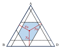
Figure 1: Probability intervals for three classes, such as those predicted by CreINNs, identify a convex set of probability distributions (a credal set, in blue) on the probability simplex (in this case, a triangle) of all probability distributions on $\mathbb{T}\!=\!\{\text{A},\text{B},\text{D}\}$. On a probability simplex, a discrete probability distribution over classes $(y_{A},y_{B},y_{D})$ is represented as a single point. The distance between each point and the edge opposite the vertex representing a class is the probability assigned to that class (red dashed lines). The probability intervals generated by our CreINNs act as constraints (parallel black dashed lines) which determine the credal set.

Note that the equality condition in (12) is met if and only if $\textstyle\overline{y}_{k}\!=\!\underline{y}_{k},\forall k\!=\!1,...,C$, indicating that the probability interval for each class collapses to a single precise value, and the network outputs a single probability vector, as is the case for DNNs. Our CreINNs are trained to learn deterministic parameter intervals, represented as $[\underline{\boldsymbol{\omega}},\overline{\boldsymbol{\omega}}]$ (described in Section 3.3), which are interpreted as the estimated bounds, given the evidence provided by the training set, for the (unknown) parameters of the ground-truth model. Therefore, neither parameter intervals nor predicted probability intervals of CreINNs collapse to point values.

Input of CreINNs: Given the standard training set $\mathbb{D}\!=\!{\{\boldsymbol{x}_{n},\boldsymbol{t}_{n}\}}_{n=1}^{N}$, the input $[\underline{\boldsymbol{x}},\overline{\boldsymbol{x}}]$ is represented as $\underline{\boldsymbol{x}}\!=\!\overline{\boldsymbol{x}}\!=\!\boldsymbol{x}$.

Class Prediction Making: Predicting classes in the form of credal sets is a typical decision-making problem under uncertainty. Motivated by the traditional maximax and maximin criteria (denoted as $\text{S}_{\text{max}}$ and $\text{S}_{\text{min}}$, respectively) Pearman (1977), we adopt the strategies for class prediction, as follows:

$$\text{S}_{\text{max}}:\operatorname*{argmax}{y_{k_{\text{max}}}},\ \text{S}_{\text{min}}:\operatorname*{argmin}{y_{k_{\text{min}}}},\forall k,$$ (13)

where $y_{k_{\text{max}}}$ and $y_{k_{\text{min}}}$ are the reachable upper and lower probability for $k^{\text{th}}$ element within $\mathbb{Q}$, and can be readily computed as follows De Campos et al. (1994):

$$\textstyle y_{k_{\text{max}}}\!\!=\!\overline{y}_{k}\wedge\left(1\!-\!\!\sum_{j\neq k}\underline{y}_{j}\right),y_{k_{\text{min}}}\!\!=\!\underline{y}_{k}\!\vee\left(1\!-\!\!\sum_{j\neq k}\overline{y}_{j}\right).$$ (14)

Uncertainty Estimation: The implementation of (7) for computing AU and EU in our CreINNs can be achieved by

$$\begin{aligned} H^{*}\!&=\!\!\operatorname*{max}_{y_{k}\!\in[\underline{y}_{k},\overline{y}_{k}]}\sum\nolimits_{k=1}^{C}\!\!-{y}_{k}\!\log_{2}\!{y_{k}}\\ H_{*}\!&=\!\!\operatorname*{min}_{y_{k}\!\in[\underline{y}_{k},\overline{y}_{k}]}\sum\nolimits_{k=1}^{C}\!\!-y_{k}\!\log_{2}\!{y_{k}}\end{aligned}\text{s.t.}\sum\nolimits_{k=1}^{C}\!y_{k}\!=\!1,$$ (15)

which can be addressed using standard solvers.

3.2 Interval Softmax Activation Function

CreINNs are specifically designed to transform the output interval scores $[\underline{\boldsymbol{a}},\overline{\boldsymbol{a}}]^{L}$ into a set of probability intervals $[\underline{\boldsymbol{y}},\overline{\boldsymbol{y}}]$ while satisfying the condition in (12). Traditional Softmax activation function is not suitable as it can not ensure that the resulting probability bounds for each class strictly adhere to $\underline{y}_{k}\leq\overline{y}_{k}$ when computing $[\underline{{\boldsymbol{y}}},\overline{{\boldsymbol{y}}}]$ as $\underline{\boldsymbol{y}}\!=\!\text{Softmax}(\underline{\boldsymbol{a}}^{L})$ and $\overline{\boldsymbol{y}}\!=\!\text{Softmax}(\overline{\boldsymbol{a}}^{L})$, respectively. Inspired by conventional Softmax, we propose a novel activation function, called Interval Softmax, defined as follows:

$$\underline{y}_{k}\!=\!\frac{e^{\underline{a}_{k}^{L}}}{\sum_{j\neq k}^{C}e^{\frac{\underline{a}_{j}^{L}\!+\!\overline{a}_{j}^{L}}{2}}\!+\!e^{\underline{a}_{k}^{L}}},\ \ \overline{{y}}_{k}\!=\!\frac{e^{\overline{a}_{k}^{L}}}{\sum_{j\neq k}^{C}e^{\frac{\underline{a}_{j}^{L}\!+\!\overline{a}_{j}^{L}}{2}}\!+\!e^{\overline{a}_{k}^{L}}},$$ (16)

where $\underline{a}_{k}^{L}$ and $\overline{a}_{k}^{L}$ are the $k^{\text{th}}$ element of $\underline{\boldsymbol{a}}^{L}$ and $\overline{\boldsymbol{a}}^{L}$, respectively. In addition to satisfying condition (12), Interval Softmax exhibits smoothness for backward propagation and retains the “set constraint” property. Detailed discussion and proof are presented in Appendix §B.

3.3 Training Procedure

Traditionally, neural networks are trained under the assumption (referred to as ASM-1 in this paper) that the distributions of testing and training data are identical. Under this assumption, the trained model corresponds to an empirical risk minimizer Hüllermeier and Waegeman (2021), namely:

$$\operatorname*{argmin}_{\boldsymbol{\omega}}\frac{1}{N}\sum\nolimits_{n}^{N}\mathcal{L}(h^{\boldsymbol{\omega}}(\boldsymbol{x}_{n}),\boldsymbol{t}_{n}),$$ (17)

where $h^{\boldsymbol{\omega}}$ denotes the model parametrized by $\boldsymbol{\omega}$. $\mathcal{L}$ typically represents the cross-entropy loss in classification tasks.

Alternatively, another assumption, referred to as ASM-2 in this paper, is proposed within the framework of distributionally robust optimization (DRO) Sagawa et al. (2020); Nam et al. (2020); Lahoti et al. (2020). ASM-2 posits the existence of an unknown divergence between training and test distributions. The training process aims to minimize the expected loss under the worst-case scenario across a pre-constructed uncertainty set of distributions. This uncertainty set encodes potential test distributions for which the model is expected to perform well. While DRO methods can impart robustness to a broad range of distributional shifts, they may result in overly pessimistic models that optimize for improbable worst-case distributions Sagawa et al. (2020). Generally, the training process assumes the form Huang et al. (2022):

$$\begin{aligned} \operatorname*{argmin}_{\boldsymbol{\omega}}\!\frac{1}{N}\!\sum\nolimits_{n}^{N}\!\!\operatorname*{max}_{{\color[rgb]{0,0,0}\boldsymbol{\theta}_{n}\in\mathbb{S}}}\boldsymbol{\theta}_{n}\mathcal{L}(h^{\boldsymbol{\omega}}(\boldsymbol{x}_{n}),\boldsymbol{t}_{n})\ \text{s.t.}\!\sum\nolimits_{n}^{N}\!\!\!\boldsymbol{\theta}_{n}\!=\!1\end{aligned},$$ (18)

where $\boldsymbol{\theta}$ is a weight vector with length $N$ and belongs to pre-defined space $\mathbb{S}$ that is different across distinct methods Sagawa et al. (2020); Nam et al. (2020); Lahoti et al. (2020).

As the estimation of $\boldsymbol{\theta}$ in (18) is not straightforward when using batch-wise optimization, a study Huang et al. (2022) has recently proposed a heuristic: For each training batch, samples with high losses are selected through forward propagation and then utilized to update the parameters. The rationale behind this heuristic is as follows: within a batch, the samples that exhibit the highest loss are treated as hard-to-learn instances, considered as the “minority” within the training set Huang et al. (2022). Incorporating these hard-to-learn samples during training serves to enhance the distributional generalization capacity of neural networks.

In CreINNs, we correlate $\overline{\boldsymbol{y}}$ with ASM-1 while associating $\underline{\boldsymbol{y}}$ with ASM-2. Two assumptions are in turn associated with two separate components of the loss function, as follows:

$$\begin{aligned} &\mathcal{L}_{\text{cre}}\!\!=\!\!\underbrace{\frac{1}{N}\!\!\sum\nolimits_{n}^{N}\!\!\mathcal{L}(\overline{\boldsymbol{y}}_{n},\!\boldsymbol{t}_{n})}_{\mathcal{L}_{a}}\!+\!\underbrace{\frac{1}{N}\!\!\sum\nolimits_{n}^{N}\!\operatorname*{max}_{\color[rgb]{0,0,0}\boldsymbol{\theta}_{n}\in\mathbb{S}}\boldsymbol{\theta}_{n}\mathcal{L}(\underline{\boldsymbol{y}}_{n},\!\boldsymbol{t}_{n})}_{\mathcal{L}_{b}}\\ &\quad\quad\quad\text{s.t.}\textstyle\sum_{n}^{N}\!\boldsymbol{\theta}_{n}=1\ \text{and}\ \underline{\boldsymbol{\omega}}\!\leq\!\overline{\boldsymbol{\omega}}\end{aligned}.$$ (19)

As aforementioned, ASM-1 typically yields optimistic estimates, as it ideally assumes no divergence between the test and training distributions. ASM-2 may lead to pessimistic predictions because it could “exaggerate” the divergence between the distributions by overemphasising on the hard-to-learn samples Huang et al. (2022). By considering these two assumptions as boundary cases, CreINNs can learn the estimated parameter bounds $[\underline{\boldsymbol{\omega}},\overline{\boldsymbol{\omega}}]$ for the (unknown) parameters of the ground-truth model caused by a lack of knowledge about the divergence between test and training distributions.

The implementation of (19) using the aforementioned heuristic for CreINN training is presented in Algorithm 1. During each training mini-batch, the CreINN computes losses $\mathcal{L}_{a}$ and $\mathcal{L}_{b}$ in (19), utilizing the categorical cross-entropy loss without modification. Analyzing the expression (10), one can find that the upper and the lower bound of the network parameter is activated exclusively for each node in the forward propagation process. Consequently, $\mathcal{L}_{a}$ and $\mathcal{L}_{b}$ consistently update disjoint sets of parameters (weights and biases) independently. Besides, the constraint $\underline{\boldsymbol{\omega}}\leq\overline{\boldsymbol{\omega}}$ is added to ensure that $[\underline{\boldsymbol{\omega}},\overline{\boldsymbol{\omega}}]$ is valid.

  Input: Training dataset $\mathbb{D}\!=\!\left\{\boldsymbol{x}_{n},\boldsymbol{t}_{n}\right\}_{n=1}^{N}$; Portion of samples used per batch $\delta$; Batch size $\eta$; Training epochs $E$

  Output: Learnable parameter intervals $[\underline{\boldsymbol{\omega}},\overline{\boldsymbol{\omega}}]$

  Initialize $\underline{\boldsymbol{\omega}}_{0}$, $\overline{\boldsymbol{\omega}}_{0}$ under constraint $\underline{\boldsymbol{\omega}}_{0}\leq\overline{\boldsymbol{\omega}}_{0}$

  for each batch of $\mathbb{D}$ do

     $\#$ Forward propagation

     Compute $\mathcal{L}_{a}$ in (19) and $\mathcal{L}(\underline{\boldsymbol{y}}_{n}\!,\boldsymbol{t}_{n})$ for each sample

     $\#$ Approximate $\mathcal{L}_{b}$ in (19) using the heuristic

     Select samples with top $\delta\!\cdot\!\eta$ highest loss related to $\underline{\boldsymbol{y}}$

     Construct $\mathcal{L}_{b}\!=\!\frac{1}{\delta\!\cdot\!\eta}\sum\nolimits_{j=1}^{\delta\!\cdot\!\eta}\mathcal{L}(\underline{\boldsymbol{y}}_{j}\!,\boldsymbol{t}_{j})$

     $\#$ Backward propagation under the heuristic

     Minimize $\mathcal{L}_{\text{cre}}\!=\!\mathcal{L}_{a}\!+\!\mathcal{L}_{b}$ under constraints $\underline{\boldsymbol{\omega}}\!\leq\!\overline{\boldsymbol{\omega}}$

  end for

Algorithm 1 Training Procedure of CreINNs

Hyperparameter $\delta\!\in\![0.5,1)$ mainly influences the range of $[\underline{\boldsymbol{\omega}},\overline{\boldsymbol{\omega}}]$ and the training budget. A larger value of $\delta$ indicates a smaller difference between $\mathcal{L}_{a}$ and $\mathcal{L}_{b}$ for parameter updating. It assumes a narrower variation of the data distributions when applying ASM-2.

3.4 Interval Batch Normalization

In modern and deep neural network architectures such as ResNet He et al. (2016), batch normalization (BN) Ioffe and Szegedy (2015) has emerged as an indispensable element. Besides, our tests have also revealed that Interval Softmax may result in a numerical overflow when the input $[\underline{\boldsymbol{a}},\overline{\boldsymbol{a}}]^{L}$ has a wide range. In order to enhance the scalability of CreINNs for large and deep architectures, and to mitigate the challenge of numerical overflow, we introduce a novel heuristic approach called Interval Batch Normalization (IBN), derived from the conventional BN methodology. The IBN transform is illustrated in Algorithm 2. For mini-batch interval-formed node activations, for instance the outputs of $l^{\text{th}}$ layer $[\underline{\boldsymbol{a}},\overline{\boldsymbol{a}}]^{l}$, the center and radius (half of the range) of each interval are computed. The mini-batch centers and radii are then normalized, respectively. Finally, the batch-normalized centers and radii are utilized to synthesize the normalized deterministic intervals. Note that the training and inference in batch-normalized CreINNs follow a similar procedure to that of traditional BN.

  Input: Mini-batch inputs: ${\left\{[{\underline{a}}_{i},{\overline{a}}_{i}]\right\}}_{i=1}^{\eta}$; Hyperparameter $\epsilon$; Trainable parameters $\gamma_{c}$, $\beta_{c}$, $\gamma_{r}$, $\beta_{r}$

  Output: $\color[rgb]{0,0,0}{\left\{{[{\underline{a}}_{\text{IBN}_{i}},\overline{a}_{\text{IBN}_{i}}]}=\text{IBN}_{\gamma_{c},\beta_{c},\gamma_{r}\beta_{r}}\left(\left[{\underline{a}}_{i},{\overline{a}}_{i}\right]\right)\right\}}_{i=1}^{\eta}$

  $\#$ Compute center and radius of intervals

  $\{c_{i}\}\!\leftarrow\!\{\frac{\underline{a}_{i}+\overline{a}_{i}}{2}\}$,   $\{r_{i}\}\!\leftarrow\!\{\frac{\overline{a}_{i}-\underline{a}_{i}}{2}\}$

  $\#$ Compute mini-batch mean and variance

  $\mu_{\mathcal{B},c}\!\leftarrow\!\frac{1}{\eta}\sum_{i=1}^{\eta}c_{i}$, $\mu_{\mathcal{B},r}\!\leftarrow\!\frac{1}{\eta}\sum_{i=1}^{\eta}r_{i}$

  $\sigma_{\mathcal{B},c}^{2}\!\leftarrow\!\frac{1}{\eta}\sum_{i=1}^{\eta}\!\!{\left(c_{i}\!-\!\mu_{\mathcal{B},c}\right)}^{2}$,  $\sigma_{\mathcal{B},r}^{2}\!\leftarrow\!\frac{1}{\eta}\sum_{i=1}^{\eta}\!\!{\left(r_{i}\!-\!\mu_{\mathcal{B},r}\right)}^{2}$

  $\#$ Normalize, scale, and shift

  $\hat{{c}_{i}}\!\leftarrow\!\frac{c_{i}-\mu_{\mathcal{B},c}}{\sqrt{\sigma_{\mathcal{B},c}^{2}+\epsilon}}$, $\hat{{r}_{i}}\!\leftarrow\!\frac{r_{i}-\mu_{\mathcal{B},r}}{\sqrt{\sigma_{\mathcal{B},r}^{2}+\epsilon}}$

  $c_{out,i}\leftarrow\gamma_{c}\hat{{c}_{i}}+\beta_{c}$, $r_{out,i}\leftarrow\gamma_{r}\hat{{r}_{i}}+\beta_{r}$

  $\#$ Generate output

  $\color[rgb]{0,0,0}{[{\underline{a}}_{\text{IBN}_{i}},\overline{a}_{\text{IBN}_{i}}]}\!\leftarrow\!\left[c_{out,i}\!-\!\left|r_{out,i}\right|,c_{out,i}\!+\!\left|r_{out,i}\right|\right]$

Algorithm 2 Interval Batch Normalization Transform

4 Experimental Validation

Setup: We evaluate the performance of CreINNs through out-of-distribution (OoD) detection benchmarks on CIFAR10 Krizhevsky et al. (2009) vs SVHN Netzer et al. (2011) datasets. Regarding baselines, we opt for two standardized variational BNNs: BNNR (Auto-Encoding variational Bayes Kingma and Welling (2013) with the local reparameterization trick Molchanov et al. (2017)) and BNNF (Flipout gradient estimator with the negative evidence lower bound loss Wen et al. (2018)). BNNs using sampling approaches are excluded for comparison due to their generally heightened computational resource requirements Gawlikowski et al. (2021); Jospin et al. (2022). Additionally, DEs are constructed by combining three DNNs trained with distinct random seeds, denoted as DE-3. All models are trained on the ResNet50 architecture with a learning rate scheduler, initialized at 0.001, and subjected to a 0.1 reduction at epochs 80, 120, 160, and 180. Standard data augmentation Cubuk et al. (2019) is uniformly applied across all approaches. The utilized devices are two Tesla P100-SXM2-16GB GPUs. Figure 2 indicates the averaged training and validation accuracy monitoring of various models over ten runs.

Evaluation metrics on uncertainty estimation: Due to the absence of ground truth values of prediction uncertainty, we employ two indirect methodologies, applied to in-distribution (InD) samples (CIFAR10) and out-of-distribution (OoD) samples (SVHN), separately.

Accuracy-rejection (AR) curves are employed for InD samples, which involves evaluating the improvement of prediction accuracy in uncertainty estimation Hühn and Hüllermeier (2008); Band et al. (2021). An AR curve depicts the model prediction accuracy as a function of the percentage of rejections in the context of selective classification. Within a batch of test data, samples with higher prediction uncertainty will be rejected first. It is observed for verified prediction uncertainty estimation that the AR curve exhibits a monotonic increase, revealing improved prediction accuracy with increasing values of rejection rate. On the contrary, AR curves present flat for random abstention Shaker and Hüllermeier (2021).

OoD detection is mainly for EU quantification wherein OoD data points are expected to exhibit greater EU than InD samples. AUROC (Area Under the Receiver Operating Characteristic curve) and AUPRC (Area Under the Precision-Recall curve) scores are used as OoD detection metrics. AUROC quantifies the rates of true and false positives, whereas AUPRC evaluates precision and recall trade-offs, providing valuable insights into the model’s effectiveness across different confidence levels. Greater scores indicate higher quality of uncertainty estimation.

Results: Table 1 reports the performance comparison between various models implemented on ResNet50 architectures using CIFAR10 as InD and SVHN as OoD dataset. It illustrates that CreINNs exhibit superior test accuracy scores when employing either the $\text{S}_{\text{min}}$ or $\text{S}_{\text{max}}$ class prediction strategies. This accuracy improvements can be ascribed to the incorporation of divergence between training and test distributions during the learning process of CreINNs.

Furthermore, CreINNs outperform in terms of inference time compared to variational BNNs. This advantage arises from the fact that CreINNs utilize conventional forward and backward propagation methods. In contrast, BNNs necessitate costly model averaging techniques for capturing uncertainty in predictions, whereas CreINNs estimate uncertainty during inference without the need for sampling, rendering them suitable for real-time applications. The findings reveal that CreINNs demand a computation budget exceeding four times that of DNNs due to the intrinsic interval arithmetic in (10). The comparison of inference times is less equitable for CreINNs, as they incorporate custom layers without optimization, unlike the standardized TensorFlow models. Despite DEs-3 exhibiting optimal performance in terms of inference time, it is imperative to consider the substantial parameter quantity (model size).

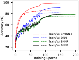
Figure 2: Training and validation accuracies, where CreINN-L represents results related to $\underline{\boldsymbol{y}}$.

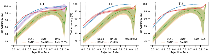
Figure 3: Accuracy-rejection curves using AU, EU and TU as uncertainty measures across distinct models. The mean and standard deviation (STD) values are derived from ten independent and identical runs. Regarding results of variational BNNs, we set $N_{p}\!=\!5$.

In the context of uncertainty estimation on InD samples, Figure 3 substantiates the efficacy of CreINNs in estimating AU, EU, and TU by illustrating a positive correlation between accuracy and rejection rate. From a practical perspective, when adopting a rejection rate of 0.05 Malinin et al. (2021), CreINNs exhibit superior performance compared to alternative methods.

In the realm of OoD detection, CreINNs stand out for EU estimation, as evidenced by their superior AUROC and AUPRC values when compared to alternative methods, as shown in Table 1. Additionally, we evaluated TU estimation, a widely employed metric in conjunction with BNNs and DEs Band et al. (2021). Notably, CreINNs exhibited outperformance in this aspect as well. The enhanced performance of CreINNs on OoD detection can be primarily ascribed to their utilization of credal sets for modeling uncertainty within predictions. Credal sets inherently amalgamate sets and distributions within a consistent framework, thereby exhibiting a heightened capability to capture EU through the assessment of non-specificity across distributions Hüllermeier and Waegeman (2021).

						OoD Detection (%, ↑)
	Model	Test accuracy (%, ↑)		Inference time (ms)	Params. (million)		AUROC	AUPRC
	DNN	80.77 ± 1.15		60.9 ± 0.5	23.61	AU	74.88 ± 2.16	83.58 ± 1.61
						TU	76.81 ± 0.95	84.57 ± 0.94
	DEs-3	83.76 ± 0.49		179.1 ± 1.2	70.82	EU	75.21 ± 1.23	84.51 ± 0.96
		${N_{p}\!\!=\!\!1}$	75.53 ± 1.76	731.7 ± 149.2		TU	74.86 ± 2.45	83.30 ± 1.79
	BNNR	${N_{p}\!\!=\!\!5}$	75.67 ± 1.74	3489.5 ± 79.4	47.11	EU	72.71 ± 3.26	83.78 ± 2.32
		${N_{p}\!\!=\!\!1}$	75.48 ± 2.41	810.3 ± 69.9		TU	76.04 ± 1.54	84.01 ± 1.06
	BNNF	${N_{p}\!\!=\!\!5}$	75.56 ± 2.38	3981.7 ± 70.6	47.11	EU	73.26 ± 2.17	83.76 ± 1.77
		$\text{S}_{\text{min}}$	85.03 ± 0.14			TU	83.53 ± 1.23	91.48 ± 0.55
CIFAR10	CreINN	$\text{S}_{\text{max}}$	85.03 ± 0.14	278.1 ± 1.9	47.21	EU	80.64 ± 1.83	89.00 ± 1.85

Table 1: Performance comparison across various models on ResNet50 architectures on CIFAR10 dataset from ten independent and identical runs. Inference time is measured using single Tesla P100 GPU. Regarding OoD detection, SVHN are the OoD samples.

Ablation study on hyperparameter $\delta$: In this test, we train CreINNs on the ResNet50 architecture under same training configuration, where only hyperparameter $\delta$ is varied across values of 0.5, 0.75, and 0.875. The results presented in Figure 4 showcase a performance comparison regarding test accuracy, as well as AUROC and AUPRC scores, utilizing TU and EU as metrics for OoD detection. The quantitative evidence affirms the robustness of CreINNs’ uncertainty estimation across diverse hyperparameter settings.

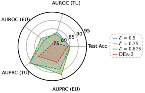
Figure 4: Test accuracy (%) and OoD detection performance (%) of CreINNs using different values of hyperparameter $\delta$ for training.

5 Conclusion and Future Work

In this study, we present innovative CreINNs designed for uncertainty estimation in classification tasks. CreINNs preserve the foundational structure of conventional INNs and articulate parameter uncertainty through deterministic intervals. They yield predictions in the form of credal sets within the mathematical framework of probability intervals. In contrast to variational BNNs and DEs, CreINNs exhibit superior EU estimation on OoD detection benchmarks when employing deep architectures like ResNet50. Moreover, CreINNs showcase a noteworthy reduction in computational complexity compared to variational BNNs during the inference phase, and they boast smaller model sizes than DEs.

Limitation and Future Work: Our future research endeavors will focus on reducing computational complexity, for instance considering sparsity. Moreover, our forthcoming efforts will be dedicated to the development of a comprehensive and direct evaluation framework for various uncertainty-aware models, leveraging practical and challenging datasets. Furthermore, we aspire to deepen our understanding of CreINNs by delving into aspects such as optimizing hyperparameters and evaluating their suitability for handling interval input data in real-world scenarios and industrial applications.

Appendix A Forward Propagation of Classical INNs

Fig. 5 illustrate the structure of classical INNs. By analyzing all potential results of calculating $[\underline{\boldsymbol{o}},\overline{\boldsymbol{o}}]$ in (8) under various conditions (positivity/negativity) over $\underline{\boldsymbol{a}},\overline{\boldsymbol{a}}$ and $\underline{\boldsymbol{W}},\overline{\boldsymbol{W}}$, the calculation of $[\underline{\boldsymbol{o}},\overline{\boldsymbol{o}}]$ during the forward propagation of classical INNs can be reformulated as follows:

$$\begin{aligned} \underline{\boldsymbol{o}}&\!=\!\text{min}\{\overline{\boldsymbol{W}},\boldsymbol{0}\}\!\cdot\!\text{min}\{\overline{\boldsymbol{a}},\boldsymbol{0}\}\!+\!\text{max}\{\underline{\boldsymbol{W}},\boldsymbol{0}\}\!\cdot\!\text{max}\{\underline{\boldsymbol{a}},\boldsymbol{0}\}\\ &\!+\!\text{min}\{\text{max}\{\overline{\boldsymbol{W}},\boldsymbol{0}\}\!\cdot\!\text{min}\{\underline{\boldsymbol{a}},\boldsymbol{0}\}\!-\!\text{min}\{\underline{\boldsymbol{W}},\boldsymbol{0}\}\\ &\!\cdot\!\text{max}\{\overline{\boldsymbol{a}},\boldsymbol{0}\},\boldsymbol{0}\}\!+\!\text{min}\{\underline{\boldsymbol{W}},\boldsymbol{0}\}\!\cdot\!\text{max}\{\overline{\boldsymbol{a}},\boldsymbol{0}\}\\ \overline{\boldsymbol{o}}&\!=\!\text{min}\{\overline{\boldsymbol{W}},\boldsymbol{0}\}\!\cdot\!\text{max}\{\underline{\boldsymbol{a}},\boldsymbol{0}\}\!+\!\text{max}\{\underline{\boldsymbol{W}},\boldsymbol{0}\}\!\cdot\!\text{min}\{\overline{\boldsymbol{a}},\boldsymbol{0}\}\\ &\!+\!\text{max}\{\text{min}\{\underline{\boldsymbol{W}},\boldsymbol{0}\}\!\cdot\!\text{min}\{\underline{\boldsymbol{a}},\boldsymbol{0}\}\!-\!\text{max}\{\overline{\boldsymbol{W}},\boldsymbol{0}\}\\ &\!\cdot\!\text{max}\{\overline{\boldsymbol{a}},\boldsymbol{0}\},\boldsymbol{0}\}\!+\!\text{max}\{\overline{\boldsymbol{W}},\boldsymbol{0}\}\!\cdot\!\text{max}\{\overline{\boldsymbol{a}},\boldsymbol{0}\}\end{aligned},$$ (20)

in which $\boldsymbol{0}$ is a zero matrix or vector having the same dimension with the quantities in the same min or max operation.

The functions in (20) are continuous, although they are not strictly differentiable at zeros. Therefore, the smoothness of forward propagation of INNs ensures that parameter updates are attainable in the same way as standard neural networks Oala et al. [2021].

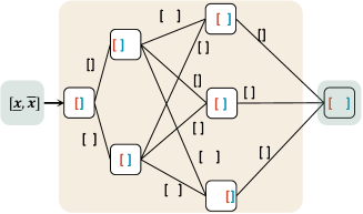
Figure 5: In a traditional INN, the output of each computing node is a closed interval of real values (color square brackets) and is propagated through the layers via interval-valued parameters (black square brackets), using interval arithmetic .

Appendix B Detailed Discussion on Interval Softmax

Recall that the probability intervals $[\underline{\boldsymbol{y}},\overline{\boldsymbol{y}}]\!=\!\{[\underline{y}_{k},\overline{y}_{k}]\}_{k=1}^{C}$ can be calculated from the real-number intervals $[\underline{\boldsymbol{a}},\overline{\boldsymbol{a}}]^{L}\!=\!\{[\underline{a}_{k}^{L},\overline{a}_{k}^{L}]\}_{k=1}^{C}$ by using Interval Softmax activation in (16). Interval Softmax reduces to the standard Sigmoid for binary classification, given as follows:

$$\underline{y}\!=\!\frac{1}{1+e^{-\underline{a}^{L}}},\ \ \overline{y}\!=\!\frac{1}{1+e^{-\overline{a}^{L}}}.$$ (21)

The proof of Interval Softmax satisfying the convex condition in (12) is provided as follows:

$$\sum\limits_{k=1}^{C}\underline{y}_{k}\!=\!\!\sum\limits_{k=1}^{C}\dfrac{e^{\underline{a}_{k}^{L}}}{\!\sum\limits_{j\neq k}^{C}e^{\frac{\underline{a}_{j}^{L}\!+\!\overline{a}_{j}^{L}}{2}}\!+\!e^{\underline{a}_{k}^{L}}}\!\leq\!\!\sum\limits_{k=1}^{C}\!\dfrac{e^{\frac{\underline{a}_{k}^{L}\!+\!\overline{a}_{k}^{L}}{2}}}{\sum\limits_{j\neq k}^{C}\!e^{\frac{\underline{a}_{j}^{L}\!+\!\overline{a}_{j}^{L}}{2}}\!+\!e^{\frac{\underline{a}_{k}^{L}\!+\!\overline{a}_{k}^{L}}{2}}}$$ (22)

$$=\!1\!\leq\sum\limits_{k=1}^{C}\!\dfrac{e^{\overline{a}_{k}^{L}}}{\sum\limits_{j\neq k}^{C}e^{\frac{\underline{a}_{j}^{L}\!+\!\overline{a}_{j}^{L}}{2}}\!+\!e^{\overline{a}_{k}^{L}}}\!=\!\sum\limits_{k=1}^{C}\overline{y}_{k}.$$

Interval Softmax demonstrates smoothness during backward propagation, and relative partial derivative calculations can be derived as follows:

$$\frac{\partial\underline{y}_{k}}{\partial\underline{a}_{j}^{L}}=\left\{\begin{array}[]{ll}\underline{y}_{k}\!\cdot\!(1-\underline{y}_{k}),&k=j\\ -\frac{1}{2}\!\cdot\!\underline{y}_{k}\!\cdot\!\frac{e^{\frac{a_{j}^{L}+\bar{a}_{j}^{L}}{2}}}{\sum_{j\neq k}^{c}e^{\frac{a_{j}^{L}+\bar{a}_{j}^{L}}{2}}+e^{\underline{a}_{k}^{L}}}&k\neq j\end{array}\right.$$ (25)

$$\frac{\partial\underline{y}_{k}}{\partial\overline{a}_{j}^{L}}=\left\{\begin{array}[]{ll}0,&k=j\\ -\frac{1}{2}\!\cdot\!\underline{y}_{k}\!\cdot\!\frac{e^{\frac{a_{j}^{L}+\bar{a}_{j}^{L}}{2}}}{\sum_{j\neq k}^{c}e^{\frac{a_{j}^{L}+\bar{a}_{j}^{L}}{2}}+e^{\underline{a}_{k}^{L}}}&k\neq j\end{array}\right.$$ (28)

$$\frac{\partial\overline{y}_{k}}{\partial\overline{a}_{j}^{L}}=\left\{\begin{array}[]{ll}\overline{y}_{k}\!\cdot\!(1-\overline{y}_{k}),&k=j\\ -\frac{1}{2}\!\cdot\!\overline{y}_{k}\!\cdot\!\frac{e^{\frac{a_{j}^{L}+\bar{a}_{j}^{L}}{2}}}{\sum_{j\neq k}^{c}e^{\frac{a_{j}^{L}+\bar{a}_{j}^{L}}{2}}+e^{\underline{a}_{k}^{L}}}&k\neq j\end{array}\right.$$ (31)

$$\frac{\partial\overline{y}_{k}}{\partial\underline{a}_{j}^{L}}=\left\{\begin{array}[]{ll}0,&k=j\\ -\frac{1}{2}\!\cdot\!\overline{y}_{k}\!\cdot\!\frac{e^{\frac{a_{j}^{L}+\bar{a}_{j}^{L}}{2}}}{\sum_{j\neq k}^{c}e^{\frac{a_{j}^{L}+\bar{a}_{j}^{L}}{2}}+e^{\underline{a}_{k}^{L}}}&k\neq j\end{array}\right.$$ (34)

Additionally, the property of “set constraint” remains satisfied. Namely, for any $a_{k}^{L}\!\in\![\underline{a}_{k},\overline{a}_{k}]^{L}$, the condition in (35) consistently holds.

$$y_{k}\!=\!\frac{e^{a_{k}^{L}}}{\sum_{j\neq k}^{C}e^{\frac{\underline{a}_{j}^{L}\!+\!\overline{a}_{j}^{L}}{2}}\!+\!e^{a_{k}^{L}}}\!\in\![\underline{y}_{k},\overline{y}_{k}].$$ (35)

By the property of “set constraint” shown in (9) and (35), we can find it: Given an instance $\boldsymbol{x}\!\in\!\mathbb{X}$, the CreINN implicitly and effectively produces a set of DNNs denoted as $h^{*}$, which are characterized by parameters ${\boldsymbol{\omega}}^{*}\in[\underline{\boldsymbol{\omega}},\overline{\boldsymbol{\omega}}]$. The prediction of each DNN, represented as $\boldsymbol{y}^{*}\!=\!h^{*}(\boldsymbol{x})$, is a single probability vector, and each predicted value $y^{*}_{k}$ for the $k^{\text{th}}$ class falls within the range $[\underline{y}_{k},\overline{y}_{k}]$ predicted by the CreINN.

References

- Abdar et al. [2021] Moloud Abdar, Farhad Pourpanah, Sadiq Hussain, Dana Rezazadegan, Li Liu, Mohammad Ghavamzadeh, Paul Fieguth, Xiaochun Cao, Abbas Khosravi, U Rajendra Acharya, et al. A review of uncertainty quantification in deep learning: Techniques, applications and challenges. Information Fusion, 76:243–297, 2021.
- Abe et al. [2022] Taiga Abe, Estefany Kelly Buchanan, Geoff Pleiss, Richard Zemel, and John P Cunningham. Deep ensembles work, but are they necessary? Advances in Neural Information Processing Systems, 35:33646–33660, 2022.
- Abellán et al. [2006] Joaquín Abellán, George J Klir, and Serafín Moral. Disaggregated total uncertainty measure for credal sets. International Journal of General Systems, 35(1):29–44, 2006.
- Band et al. [2021] Neil Band, Tim GJ Rudner, Qixuan Feng, Angelos Filos, Zachary Nado, Michael W Dusenberry, Ghassen Jerfel, Dustin Tran, and Yarin Gal. Benchmarking bayesian deep learning on diabetic retinopathy detection tasks. In Proceedings of Conference on Neural Information Processing Systems Datasets and Benchmarks Track (Round 2), 2021.
- Blundell et al. [2015] Charles Blundell, Julien Cornebise, Koray Kavukcuoglu, and Daan Wierstra. Weight uncertainty in neural network. In Proceedings of the International Conference on Machine Learning, pages 1613–1622. PMLR, 2015.
- Caprio et al. [2023] Michele Caprio, Souradeep Dutta, Kuk Jin Jang, Vivian Lin, Radoslav Ivanov, Oleg Sokolsky, and Insup Lee. Imprecise Bayesian neural networks. arXiv preprint arXiv:2302.09656, 2023.
- Cattaneo and Wiencierz [2012] Marco EGV Cattaneo and Andrea Wiencierz. Likelihood-based imprecise regression. International Journal of Approximate Reasoning, 53(8):1137–1154, 2012.
- Ciosek et al. [2019] Kamil Ciosek, Vincent Fortuin, Ryota Tomioka, Katja Hofmann, and Richard Turner. Conservative uncertainty estimation by fitting prior networks. In International Conference on Learning Representations, 2019.
- Corani and Zaffalon [2008] Giorgio Corani and Marco Zaffalon. Learning reliable classifiers from small or incomplete data sets: The naive credal classifier 2. Journal of Machine Learning Research, 9(4), 2008.
- Corani et al. [2012] Giorgio Corani, Alessandro Antonucci, and Marco Zaffalon. Bayesian networks with imprecise probabilities: Theory and application to classification. Data Mining: Foundations and Intelligent Paradigms: Volume 1: Clustering, Association and Classification, pages 49–93, 2012.
- Cubuk et al. [2019] Ekin D Cubuk, Barret Zoph, Dandelion Mane, Vijay Vasudevan, and Quoc V Le. Autoaugment: Learning augmentation strategies from data. In Proceedings of the IEEE/CVF conference on computer vision and pattern recognition, pages 113–123, 2019.
- De Campos et al. [1994] Luis M. De Campos, Juan F. Huete, and Serafin Moral. Probability intervals: A tool for uncertain reasoning. International Journal of Uncertainty, Fuzziness and Knowledge-Based Systems, 02(02):167–196, June 1994.
- Depeweg et al. [2018] Stefan Depeweg, Jose-Miguel Hernandez-Lobato, Finale Doshi-Velez, and Steffen Udluft. Decomposition of uncertainty in bayesian deep learning for efficient and risk-sensitive learning. In International Conference on Machine Learning, pages 1184–1193. PMLR, 2018.
- Fort and Jastrzebski [2019] Stanislav Fort and Stanislaw Jastrzebski. Large scale structure of neural network loss landscapes. Advances in Neural Information Processing Systems, 32, 2019.
- Gal and Ghahramani [2016] Yarin Gal and Zoubin Ghahramani. Dropout as a Bayesian approximation: Representing model uncertainty in deep learning. In Proceedings of the International Conference on Machine Learning, pages 1050–1059. PMLR, 2016.
- Garczarczyk [2000] Z.A. Garczarczyk. Interval neural networks. In Proceedings of the IEEE International Symposium on Circuits and Systems, volume 3, pages 567–570 vol.3, 2000.
- Gawlikowski et al. [2021] Jakob Gawlikowski, Cedrique Rovile Njieutcheu Tassi, Mohsin Ali, Jongseok Lee, Matthias Humt, Jianxiang Feng, Anna Kruspe, Rudolph Triebel, Peter Jung, Ribana Roscher, et al. A survey of uncertainty in deep neural networks. arXiv preprint arXiv:2107.03342, 2021.
- Gustafsson et al. [2020] Fredrik K Gustafsson, Martin Danelljan, and Thomas B Schon. Evaluating scalable bayesian deep learning methods for robust computer vision. In Proceedings of the IEEE/CVF conference on computer vision and pattern recognition workshops, pages 318–319, 2020.
- He et al. [2016] Kaiming He, Xiangyu Zhang, Shaoqing Ren, and Jian Sun. Deep residual learning for image recognition. In Proceedings of the IEEE conference on computer vision and pattern recognition, pages 770–778, 2016.
- He et al. [2020] Bobby He, Balaji Lakshminarayanan, and Yee Whye Teh. Bayesian deep ensembles via the neural tangent kernel. Advances in neural information processing systems, 33:1010–1022, 2020.
- Hickey et al. [2001] Timothy Hickey, Qun Ju, and Maarten H Van Emden. Interval arithmetic: From principles to implementation. Journal of the ACM (JACM), 48(5):1038–1068, 2001.
- Hoffman et al. [2014] Matthew D Hoffman, Andrew Gelman, et al. The No-U-Turn sampler: adaptively setting path lengths in Hamiltonian Monte Carlo. J. Mach. Learn. Res., 15(1):1593–1623, 2014.
- Huang et al. [2022] Zeyi Huang, Haohan Wang, Dong Huang, Yong Jae Lee, and Eric P Xing. The two dimensions of worst-case training and their integrated effect for out-of-domain generalization. In Proceedings of the IEEE/CVF Conference on Computer Vision and Pattern Recognition, pages 9631–9641, 2022.
- Hühn and Hüllermeier [2008] Jens Christian Hühn and Eyke Hüllermeier. Fr3: A fuzzy rule learner for inducing reliable classifiers. IEEE Transactions on Fuzzy Systems, 17(1):138–149, 2008.
- Hüllermeier and Waegeman [2021] Eyke Hüllermeier and Willem Waegeman. Aleatoric and epistemic uncertainty in machine learning: An introduction to concepts and methods. Machine Learning, 110(3):457–506, 2021.
- Hüllermeier et al. [2022] Eyke Hüllermeier, Sébastien Destercke, and Mohammad Hossein Shaker. Quantification of credal uncertainty in machine learning: A critical analysis and empirical comparison. In Proceedings of the Uncertainty in Artificial Intelligence, pages 548–557. PMLR, 2022.
- Ioffe and Szegedy [2015] Sergey Ioffe and Christian Szegedy. Batch normalization: Accelerating deep network training by reducing internal covariate shift. In Proceedings of the International Conference on Machine Learning, pages 448–456. PMLR, 2015.
- Jospin et al. [2022] Laurent Valentin Jospin, Hamid Laga, Farid Boussaid, Wray Buntine, and Mohammed Bennamoun. Hands-on Bayesian neural networks—A tutorial for deep learning users. IEEE Computational Intelligence Magazine, 17(2):29–48, 2022.
- Kendall and Gal [2017] Alex Kendall and Yarin Gal. What uncertainties do we need in bayesian deep learning for computer vision? Advances in neural information processing systems, 30, 2017.
- Kingma and Welling [2013] Diederik P Kingma and Max Welling. Auto-encoding variational Bayes. arXiv preprint arXiv:1312.6114, 2013.
- Kowalski and Kulczycki [2017] Piotr A Kowalski and Piotr Kulczycki. Interval probabilistic neural network. Neural Computing and Applications, 28(4):817–834, 2017.
- Krizhevsky et al. [2009] Alex Krizhevsky, Vinod Nair, and Geoffrey Hinton. Cifar-10 (canadian institute for advanced research). 2009.
- Kruse et al. [2022] Rudolf Kruse, Sanaz Mostaghim, Christian Borgelt, Christian Braune, and Matthias Steinbrecher. Multi-layer perceptrons. In Computational intelligence: a methodological introduction, pages 53–124. Springer, 2022.
- Lahoti et al. [2020] Preethi Lahoti, Alex Beutel, Jilin Chen, Kang Lee, Flavien Prost, Nithum Thain, Xuezhi Wang, and Ed Chi. Fairness without demographics through adversarially reweighted learning. Advances in Neural Information Processing Systems, 33:728–740, 2020.
- Lakshminarayanan et al. [2017] Balaji Lakshminarayanan, Alexander Pritzel, and Charles Blundell. Simple and scalable predictive uncertainty estimation using deep ensembles. Advances in Neural Information Processing Systems, 30, 2017.
- Lambrou et al. [2010] Antonis Lambrou, Harris Papadopoulos, and Alex Gammerman. Reliable confidence measures for medical diagnosis with evolutionary algorithms. IEEE Transactions on Information Technology in Biomedicine, 15(1):93–99, 2010.
- Levi [1980] Isaac Levi. The enterprise of knowledge: An essay on knowledge, credal probability, and chance. MIT press, 1980.
- Liu et al. [2020] Jeremiah Liu, Zi Lin, Shreyas Padhy, Dustin Tran, Tania Bedrax Weiss, and Balaji Lakshminarayanan. Simple and principled uncertainty estimation with deterministic deep learning via distance awareness. Advances in Neural Information Processing Systems, 33:7498–7512, 2020.
- Malinin et al. [2021] Andrey Malinin, Neil Band, Yarin Gal, Mark Gales, Alexander Ganshin, German Chesnokov, Alexey Noskov, Andrey Ploskonosov, Liudmila Prokhorenkova, Ivan Provilkov, et al. Shifts: A dataset of real distributional shift across multiple large-scale tasks. In Proceedings of Conference on Neural Information Processing Systems Datasets and Benchmarks Track (Round 2), 2021.
- Manchingal and Cuzzolin [2022] Shireen Kudukkil Manchingal and Fabio Cuzzolin. Epistemic deep learning. arXiv preprint arXiv:2206.07609, 2022.
- Molchanov et al. [2017] Dmitry Molchanov, Arsenii Ashukha, and Dmitry Vetrov. Variational dropout sparsifies deep neural networks. In Proceedings of the International Conference on Machine Learning, pages 2498–2507. PMLR, 2017.
- Moral-García and Abellán [2021] Serafín Moral-García and Joaquín Abellán. Credal sets representable by reachable probability intervals and belief functions. International Journal of Approximate Reasoning, 129:84–102, 2021.
- Nam et al. [2020] Junhyun Nam, Hyuntak Cha, Sungsoo Ahn, Jaeho Lee, and Jinwoo Shin. Learning from failure: De-biasing classifier from biased classifier. Advances in Neural Information Processing Systems, 33:20673–20684, 2020.
- Neal and others [2011] Radford M Neal et al. MCMC using Hamiltonian dynamics. Handbook of Markov Chain Monte Carlo, 2(11):2, 2011.
- Netzer et al. [2011] Yuval Netzer, Tao Wang, Adam Coates, Alessandro Bissacco, Bo Wu, and Andrew Y Ng. Reading digits in natural images with unsupervised feature learning. 2011.
- Oala et al. [2021] Luis Oala, Cosmas Heiß, Jan Macdonald, Maximilian März, Gitta Kutyniok, and Wojciech Samek. Detecting failure modes in image reconstructions with interval neural network uncertainty. International Journal of Computer Assisted Radiology and Surgery, 16(12):2089–2097, 2021.
- Ovadia et al. [2019] Yaniv Ovadia, Emily Fertig, Jie Ren, Zachary Nado, David Sculley, Sebastian Nowozin, Joshua Dillon, Balaji Lakshminarayanan, and Jasper Snoek. Can you trust your model’s uncertainty? evaluating predictive uncertainty under dataset shift. Advances in neural information processing systems, 32, 2019.
- Pearman [1977] AD Pearman. A weighted maximin and maximax approach to multiple criteria decision making. Journal of the Operational Research Society, 28(3):584–587, 1977.
- Sagawa et al. [2020] Shiori Sagawa, Pang Wei Koh, Tatsunori B. Hashimoto, and Percy Liang. Distributionally robust neural networks. In Proceedings of the International Conference on Learning Representations, 2020.
- Sale et al. [2023] Yusuf Sale, Michele Caprio, and Eyke Höllermeier. Is the volume of a credal set a good measure for epistemic uncertainty? In Uncertainty in Artificial Intelligence, pages 1795–1804. PMLR, 2023.
- Senge et al. [2014] Robin Senge, Stefan Bösner, Krzysztof Dembczyński, Jörg Haasenritter, Oliver Hirsch, Norbert Donner-Banzhoff, and Eyke Hüllermeier. Reliable classification: Learning classifiers that distinguish aleatoric and epistemic uncertainty. Information Sciences, 255:16–29, 2014.
- Shaker and Hüllermeier [2021] Mohammad Hossein Shaker and Eyke Hüllermeier. Ensemble-based uncertainty quantification: Bayesian versus credal inference. In PROCEEDINGS 31. WORKSHOP COMPUTATIONAL INTELLIGENCE, volume 25, page 63, 2021.
- Shannon [1948] Claude Elwood Shannon. A mathematical theory of communication. The Bell system technical journal, 27(3):379–423, 1948.
- Tretiak et al. [2023] Krasymyr Tretiak, Georg Schollmeyer, and Scott Ferson. Neural network model for imprecise regression with interval dependent variables. Neural Networks, 161:550–564, 2023.
- Wen et al. [2018] Yeming Wen, Paul Vicol, Jimmy Ba, Dustin Tran, and Roger Grosse. Flipout: Efficient pseudo-independent weight perturbations on mini-batches. In Proceedings of the International Conference on Learning Representations, 2018.
- Zaffalon [2002] Marco Zaffalon. The naive credal classifier. Journal of statistical planning and inference, 105(1):5–21, 2002.