Basic fractional nonlinear-wave models and solitons

Abstract

This review article provides a concise summary of one- and two-dimensional models for the propagation of linear and nonlinear waves in fractional media. The basic models, which originate from the Laskin’s fractional quantum mechanics and more experimentally relevant setups emulating fractional diffraction in optics, are based on the Riesz definition of fractional derivatives, which are characterized by the respective Lévy indices. Basic species of one-dimensional solitons, produced by the fractional models which include cubic or quadratic nonlinear terms, are outlined too. In particular, it is demonstrated that the variational approximation is relevant in many cases. A summary of the recently demonstrated experimental realization of the fractional group-velocity dispersion in fiber lasers is also presented.

The paper is devoted to the celebration of the 80th birthday of David K. Campbell.

The formal calculus based on the concept of fractional derivatives is a branch of formal mathematics that has been known in the course of ca. 200 years. Ca. 20 years ago, this concept had appeared in physics as an ingredient of fractional quantum mechanics, which is based on the Schrödinger equation with the fractional operator of kinetic energy, for the wave function of particles which, in their classical form, move by random Lévy flights. The fractionality of the Schrödinger equations of this type is characterized by the Lévy index (LI) $\alpha$, which takes values $0<\alpha\leq 2$. It determines the form of the fractional kinetic-energy operator, as $\left(-\partial^{2}/\partial x^{2}\right)^{\alpha/2}$, the usual (nonfractional) quantum mechanics corresponding to $\alpha=2$. While fractional quantum mechanics remains far from experimental implementation, much interest has been drawn to the more recent proposal to emulate the fractional diffraction, modeled by the same equations, by means of the wave propagation in specially devised optical cavities. Many theoretical results have been reported for solitons, vortices and other modes supported by the respective fractional Schrödinger equations which include cubic or quadratic optical nonlinearities. Very recently, the first experimental implementation of the effective fractional group-velocity dispersion has been reported for the light propagation in a fiber-laser cavity. The great deal of the current interest to these theoretical and experimental studies suggest relevance of providing a summary of the state of art in the area. Such a concise summary is offered by this article, which outlines basic models of the fractional wave propagation, and a brief overview of basic species of solitons produced by these models.

I Introduction: the concept of fractional-order derivatives

Ordinary derivatives are the central concept of the classical calculus, which has been the mathematical basis of modern science in the course of the last 350 years. In addition to the commonly known definition of derivatives of integer orders, mathematical curiosity suggested attempts to introduce derivatives of fractional orders. For example, the Darrieus-Landau instability of plane combustion fronts, propagating in a premixed gas, is determined by the linear dispersion relation between the instability growth rate $\gamma$ and wavenumber $k$ of one-dimensional (1D) perturbations corrugating the flat combustion front,

$$\gamma=C|k|,$$ (1)

with a constant $C>0$ [1]. In Eq. (1, $|k|$ implies that the same instability gain is produced by right- and left-traveling perturbations. In the framework of the phenomenological model [2], one can introduce a model equation for a real order parameter $u\left(x,t\right)$ which corresponds to the dispersion relation (1),

$$\frac{\partial u}{\partial t}=C\sqrt{-\frac{\partial^{2}}{\partial x^{2}}}u,$$ (2)

where $\sqrt{-\partial^{2}/\partial x^{2}}$is an operator that gives rise to factor $|k|$ in the Fourier space, where $k$ is the wavenumber conjugate to the spatial coordinate $x$ running along the flat combustion front. Similarly, 2D perturbations with wave vector $\mathbf{k}=\left(k_{x},k_{y}\right)$ give rise to the instability dispersion relation

$$\gamma=C|\mathbf{k}|,$$ (3)

which suggests to introduce the respective 2D phenomenological equation,

$$\frac{\partial u}{\partial t}=C\sqrt{-\frac{\partial^{2}}{\partial x^{2}}-\frac{\partial^{2}}{\partial y^{2}}}u\equiv\sqrt{-\Delta}u,$$ (4)

where $\Delta$ is the usual 2D Laplacian acting on coordinates $\left(x,y\right)$ on the flat combustion front.

It is shown in detail below that, while there are different formal definitions of fractional differential operators, such as the one $\sqrt{-\Delta}$ in Eq. (4), the definitions which are relevant for the realization in physics are defined in terms of the action of the operators in the Fourier space, similar to the relation between Eqs. (2) and (1) in 1D, or between Eqs. (4) and (3) in 2D.

Much earlier than fractional derivatives have appeared in physical models, they were considered as a formal generalization of the classical calculus. In a systematic form, the concept of the fractional calculus was elaborated by Niels Henrik Abel in 1823 [3] and Joseph Liouville in 1832 [7]. The development of these concepts has led to the abstract definition of what is known as the Caputo derivative of non-integer order $\alpha$ [8, 9],

$$D_{x}^{\alpha}\psi(x)=\frac{1}{\Gamma\left(1-\{\alpha\}\right)}\int_{0}^{x}\frac{f^{\left(n\right)}(\xi)dx}{\left(x-\xi\right)^{\left\{\alpha\right\}}},$$ (5)

where $n\equiv[\alpha]+1$, $[\alpha]$ stands for the integer part of the fractional order, $\{\alpha\}\equiv\alpha-[\alpha]$ is its fractional part, $\Gamma$ is the Gamma-function, and $f^{(n)}$ is the usual derivative. Note that this definition represents the fractional derivative as integral (nonlocal) operator, rather than as a differential one. As shown below, the fractional derivatives which appear in models originating in physics are defined differently, namely, as Riesz derivatives [10], see Eqs. (9) and (14) in Section 2.

This paper aims to produce a concise overview of linear and nonlinear dynamics in physically relevant models of fractional media. Also included is a summary of the first experimental realization of the concept of the fractional derivatives, in the form of a fiber cavity which emulates fractional group-velocity dispersion (GVD) [11]. The presentation is not comprehensive; in particular, while the main objective is to introduce models of linear and nonlinear fractional media which are relevant to physics, the summary of soliton solutions amounts to the presentation of a few examples, many other cases being only briefly mentioned. An earlier review of theoretical results for solitons in fractional models is provided in Ref. [12].

II The advent of fractional calculus to physics: Fractional quantum mechanics

For the first time, fractional derivatives had appeared in the context of physically relevant models as the mathematical basis of fractional quantum mechanics. This theory was introduced by Laskin [13, 14] for nonrelativistic particles which move, at the classical level, by Lévy flights (random leaps).

II.1 Classical particles moving by Lévy flights

The starting point for the development of fractional quantum mechanics is to consider particles whose classical stochastic motion is performed as a chain of random leaps (“Lévy flights”), rather than in the form of the usual Brownian random walk. In this regime, the mean distance $|x|$ of the particle, which moves by 1D “flights” from the initial position, $x=0$, grows with time $t$ as

$$|x|\sim t^{1/\alpha},$$ (6)

where the Lévy index (LI) $\alpha$ takes values

$$0<\alpha\leq 2$$ (7)

[16]. The limit value, $\alpha=2$, corresponds to the usual Brownian random walk, while at $\alpha<2$ Eq. (6) demonstrates that the Lévy flights give rise to faster growth of $|x|$ at $t\rightarrow\infty$. As concerns realizations of the Lévy flights in nature, a usual reference is to the life style of sharks in the ocean, which search for food moving by random fast swims, even if sharks are not appropriate objects for considering their motion in the quantum regime, which is the next step of the derivation, leading to the fractional Schrödinger equation (FSE)

II.2 The fractional linear Schrödinger equations for Lévy-flying particles and the fractional Riesz derivative

The derivation of an effective Schrödinger equation as a result of the quantization of a particle which moves, at the classical level, by Lévy flight was elaborated by Laskin [13, 14] (see also Ref. [15]). It is based on the fundamental formalism which defines quantum mechanics by means of the Feynman’s path integration. This formalism represents the quantum dynamics of a particle as a result of the superposition of virtual motions along all randomly chosen trajectories (paths). The superposition is defined as the integral in the space of all paths, $\sim\int\exp\left[iS(\mathrm{path})\right]d(\mathrm{path})$, where $S$ is the classical action corresponding to a particular path [17]. To apply this concept, Laskin considered the superposition of the paths which correspond not to the Brownian random walks, but to the Lévy flights. In the 1D setting, the result is FSE for wave function $\Psi\left(x,t\right)$. In the scaled form, it is written as

$$i\frac{\partial\Psi}{\partial t}=\frac{1}{2}\left(-\frac{\partial^{2}}{\partial x^{2}}\right)^{\alpha/2}\Psi+V(x)\Psi,$$ (8)

where $V(x)$ is the same external potential which appears in the usual Schrödinger equation.

A fundamentally important result of the derivation of Eq. (8) by means of the path-integral formalism is that the usual kinetic-energy operator, $-(1/2)\partial^{2}/\partial x^{2}$, which corresponds to $\alpha=2$ in Eq. (8), is replaced, at $\alpha<2$, by the fractional Riesz derivative [10], which is defined as the juxtaposition of the direct and inverse Fourier transforms ($x\rightarrow p\rightarrow x$) of the wave function,

$$\left(-\frac{\partial^{2}}{\partial x^{2}}\right)^{\alpha/2}\Psi=\frac{1}{2\pi}\int_{-\infty}^{+\infty}dp|p|^{\alpha}\int_{-\infty}^{+\infty}d\xi e^{ip(x-\xi)}\Psi(\xi).$$ (9)

This definition implies that the action of the fractional derivative, $\left(-\partial^{2}/\partial x^{2}\right)^{\alpha/2}$, in the Fourier space amounts to the straightforward multiplication: $\hat{\Psi}(p)\rightarrow|p|^{\alpha}\hat{\Psi}(p)$, where

$$\hat{\Psi}(p)=\int_{-\infty}^{+\infty}\exp\left(-ipx\right)\Psi(x)dx$$ (10)

is the Fourier transform of the wave function. In definition (9), $\alpha$ is the same LI which determines the classical Lévy flights as per Eq. (6).

Thus, the derivation of the physically relevant model, viz., FSE, leads to the relatively simple Riesz fractional derivative. As concerns “more sophisticated” varieties of fractional derivatives, defined on abstract mathematical grounds, such as the Caputo derivative (5), they do not emerge naturally in these physical contexts.

In the 2D space, the same derivation gives rise to the 2D FSE for wave function $\Psi\left(x,y,t\right)$) [14]:

$$i\frac{\partial\Psi}{\partial t}=\frac{1}{2}\left(-\frac{\partial^{2}}{\partial x^{2}}-\frac{\partial^{2}}{\partial y^{2}}\right)^{\alpha/2}\Psi+V(x,y)\Psi.$$ (11)

The fractional operator of the 2D kinetic energy is represented, in the 2D Fourier space $\left(p,q\right)$, by multiplier $\left(p^{2}+q^{2}\right)^{\alpha/2}$, i.e., its action amounts to

$$\hat{\Psi}(p,q)\rightarrow\left(p^{2}+q^{2}\right)^{\alpha/2}\hat{\Psi}(p,q),$$ (12)

where the 2D Fourier transform of the wave function

$$\hat{\Psi}(p,q)=\int\int\exp\left(-ipx-iqy\right)\Psi(x,y)dxdy,$$ (13)

cf. Eq. (10). Therefore, the action of the 2D operator in the coordinate space is defined as the juxtaposition of the direct and inverse Fourier transforms, with the multiplication as per Eq. (12) inserted between them:

$$\left(-\frac{\partial^{2}}{\partial x^{2}}-\frac{\partial^{2}}{\partial y^{2}}\right)^{\alpha/2}\Psi=\frac{1}{(2\pi)^{2}}\int\int dpdq\left(p^{2}+q^{2}\right)^{\alpha/2}\int\int d\xi d\eta e^{i\left[p(x-\xi)+iq(y-\eta)\right]}\Psi(\xi,\eta),$$ (14)

cf. the 1D equation (9).

Stationary solutions to Eq. (11), with real energy eigenvalue $\mu$ (in terms of Bose-Einstein condensates (BECs), it is the chemical potential) are looked for in the usual form,

$$\Psi\left(x,y,t\right)=e^{-i\mu t}U\left(x,y\right),$$ (15)

with real function $U$ satisfying the stationary equation,

$$\mu U=\frac{1}{2}\left(-\frac{\partial^{2}}{\partial x^{2}}-\frac{\partial^{2}}{\partial y^{2}}\right)^{\alpha/2}U+V(x,y)U,$$ (16)

or its 1D version, without coordinate $y$. It is relevant to mention that in the case of potential in the form of the harmonic oscillator, $V\left(x,y\right)=\left(\Omega^{2}/2\right)\left(x^{2}+y^{2}\right)$, the Fourier transform (13) satisfies the Fourier transform of Eq. (11), which takes the form of the usual Schrödinger equation, but written in the Fourier space [4]:

$$i\frac{\partial\hat{\Psi}}{\partial t}=-\frac{\Omega^{2}}{2}\left(\frac{\partial^{2}}{\partial p^{2}}+\frac{\partial^{2}}{\partial q^{2}}\right)\hat{\Psi}+\frac{1}{2}\left(p^{2}+q^{2}\right)^{\alpha/2}\hat{\Psi},$$ (17)

with the effective potential $(1/2)\left(p^{2}+q^{2}\right)^{\alpha/2}$, or the 1D version of this equation, in the absence of variable $q$. In particular, a solution of the 1D version of Eq. (17) with $\alpha=1$, i.e., with the effective Fourier-space potential $(1/2)|p|$, can be expressed in terms of the Airy function [4].

The fractional calculus has found another important application to physics in the form of fractional kinetics. This concept, which was elaborated by Zaslavsky et al. [5, 6], addresses, in particular, the kinetic theory, based on the fractional Fokker-Planck equations, for dynamics which may be intermediate between integrable and purely chaotic. It predicts fundamental effects such as anomalous transport and superdiffusion, and models real kinetic phenomena such as advection of particles in diverse physical settings. However, this topic is not considered in detail in the present article.

II.3 A conjecture: fractional Gross-Pitaevskii equations (FGPEs)

It is commonly known that the dynamics of BECs in ultracold atomic gases is very accurately approximated, in the framework of the mean-field theory, by the Gross-Pitaevskii equation, in the form of the Schrödinger equation for single-particle wave function $\psi$, supplemented by the cubic terms which represent the effect of inter-particle collisions [41]:

$$i\hbar\frac{\partial\psi}{\partial t}=-\frac{\hbar^{2}}{2m}\nabla^{2}\psi+V(\mathbf{r})\psi+\frac{4\pi\hbar^{2}}{m}a_{s}|\psi|^{2}\psi.$$ (18)

Here $m$ is the atomic mass, and $a_{s}$ is the scattering length which determines two-particle collisions ($a_{s}>0$ and $a_{s}<0$ correspond to repulsive and attractive interactions between the particles, respectively). An intriguing possibility is to consider a gas of bosonic particles obeying the FSE (8) or its 2D version (11). While a systematic derivation of the respective fractional Gross-Pitaevskii equation (FGPE), with the usual kinetic-energy operator in Eq. (18) replaced by its fractional counterpart defined as per Eqs. (8) or (11), remains a challenging objective, a natural expectation is that the equation sought for will take the following form, in the scaled form:

$$i\frac{\partial\Psi}{\partial t}=\frac{1}{2}\left(-\frac{\partial^{2}}{\partial x^{2}}-\frac{\partial^{2}}{\partial y^{2}}\right)^{\alpha/2}\Psi+V(x)\Psi+\sigma|\Psi|^{2}\Psi,$$ (19)

where $\sigma=+1$ or $-1$ corresponds to the self-repulsive or attractive condensate, respectively [12].

A recently elaborated example of the FGPE system is a model of a binary (two-component) fractional BEC, described by a spinor wave function with components $\left(\phi_{+},\phi_{-}\right)$, which maintains the spin-orbit coupling (SOC) between the components [42]. The respective system of coupled FGPEs in 2D is [37]

$$i\frac{\partial\phi_{+}}{\partial t} = \frac{1}{2}\left(-\frac{\partial^{2}}{\partial x^{2}}-\frac{\partial^{2}}{\partial y^{2}}\right)^{\alpha/2}\phi_{+}-(|\phi_{+}|^{2}+\gamma|\phi_{-}|^{2})\phi_{+}+\lambda\left(\frac{\partial\phi_{-}}{\partial x}-i\frac{\partial\phi_{-}}{\partial y}\right),$$

$$i\frac{\partial\phi_{-}}{\partial t} = \frac{1}{2}\left(-\frac{\partial^{2}}{\partial x^{2}}-\frac{\partial^{2}}{\partial y^{2}}\right)^{\alpha/2}\phi_{-}-(|\phi_{-}|^{2}+\gamma|\phi_{+}|^{2})\phi_{-}-\lambda\left(\frac{\partial\phi_{+}}{\partial x}+i\frac{\partial\phi_{+}}{\partial y}\right),$$

with the kinetic-energy operator defined as per Eq. (14), cf. Eq. (19). Here, the attractive sign of the nonlinear interactions is assumed, to provide a possibility to create solitons. The coefficient of the self-attraction is scaled to be $1$, while $\gamma>0$ is the relative strength of the cross-attraction between the components, and $\lambda$ is the strength of the linearly-mixing terms representing the SOC. By means of additional scaling, it is possible to set $\lambda\equiv 1/2$, while soliton states with real chemical potential $\mu$ are looked for as

$$\phi_{\pm}=e^{-i\mu t}u_{\pm}(x,y)$$ (21)

(cf. Eq. (15)), where complex stationary wave functions $u_{\pm}$ satisfy equations

$$\mu u_{+} = \frac{1}{2}\left(-\frac{\partial^{2}}{\partial x^{2}}-\frac{\partial^{2}}{\partial y^{2}}\right)^{\alpha/2}u_{+}-(|u_{+}|^{2}+\gamma|u_{-}|^{2})u_{+}+\frac{1}{2}\left(\frac{\partial u_{-}}{\partial x}-i\frac{\partial u_{-}}{\partial y}\right),$$

$$\mu u_{-} = \frac{1}{2}\left(-\frac{\partial^{2}}{\partial x^{2}}-\frac{\partial^{2}}{\partial y^{2}}\right)^{\alpha/2}u_{-}-(|u_{-}|^{2}+\gamma|u_{+}|^{2})u_{-}-\frac{1}{2}\left(\frac{\partial u_{+}}{\partial x}+i\frac{\partial u_{+}}{\partial y}\right).$$

Soliton solutions are characterized by the total norm,

$$N\equiv\int\int\left(\left|u_{+}\right|^{2}+\left|u_{-}\right|^{2}\right)dxdy.$$ (23)

It is relevant to mention that the stationary system (LABEL:u2D) can be derived from the respective Lagrangian:

$$L=\mu\int_{-\infty}^{+\infty}dx\int_{-\infty}^{+\infty}dy\left[\left|u_{+}(x,y)\right|^{2}+\left|u_{-}(x,y)\right|^{2}\right]$$

$$-\frac{1}{2\pi^{2}}\int_{0}^{+\infty}dp\int_{0}^{+\infty}dq(p^{2}+q^{2})^{\alpha/2}\int_{-\infty}^{+\infty}d\xi\int_{-\infty}^{+\infty}d\eta\int_{-\infty}^{+\infty}dx\int_{-\infty}^{+\infty}dy\cos\left[p(x-\xi)+q(y-\eta)\right]$$

$$\times\left[u_{+}^{\ast}(x,y)u_{+}(\xi,\eta)+u_{-}^{\ast}(x,y)u_{-}(\xi,\eta)\right]$$

$$-\frac{1}{2}\int_{-\infty}^{+\infty}dx\int_{-\infty}^{+\infty}dy\left[u_{+}^{\ast}\frac{\partial u_{-}}{\partial x}+u_{+}\frac{\partial u_{-}^{\ast}}{\partial x}-i\left(u_{+}^{\ast}\frac{\partial u_{-}}{\partial y}-u_{+}\frac{\partial u_{-}^{\ast}}{\partial y}\right)\right]$$

$$+\int_{-\infty}^{+\infty}dx\int_{-\infty}^{+\infty}dy\left[\frac{1}{2}\left(|u_{+}|^{4}+|u_{-}|^{4}\right)+\gamma|u_{+}|^{2}|u_{-}|^{2}\right],$$ (24)

where $\ast$ stand for the complex conjugate, and the integration with respect to $p$ and $q$ is reduced from the original domains $\left(-\infty,+\infty\right)$ to $\left(0,\infty\right)$, using the domains’ symmetry. Although expression (24) seems cumbersome, it can be used to predict solitons solutions of Eq. (LABEL:u2D) by means of the variational approximation (VA). To this end, the ansatz for the approximate solutions is adopted as

$$u_{+}=A_{+}\exp(-\beta(x^{2}+y^{2})),u_{-}=A_{-}(x+iy)\exp(-\beta(x^{2}+y^{2})),\beta>0,$$ (25)

with inverse width $1/\sqrt{\beta}$ and amplitudes $A_{\pm}$ (cf. the known version of the VA for the usual 2D nonlinear Schrödinger equation [44, 45]). The norm of ansatz (25) is $N=\left(\pi/2\beta\right)\left(A_{+}^{2}+A_{-}^{2}/(2\beta)\right)$.

The ansatz (25) represents the semi-vortex (SV) type, which implies that components $u_{+}$ and $u_{-}$ carry vorticities $0$ and $1$, respectively [43] (see an example shown by means of cross-sections of the two components in Fig. 1(b)). The SV structure is an exact feature of the 2D solitons shaped by SOC, which is not restricted by the applicability of VA.

The substitution of ansatz (25) in Lagrangian (24) produces the respective effective Lagrangian,

$$L_{\mathrm{eff}}=\mu N-\frac{\pi\Gamma\left(1+\alpha/2\right)}{2\left(2\beta\right)^{1-\alpha/2}}\left[A_{+}^{2}+\left(1+\frac{\alpha}{2}\right)\frac{A_{-}^{2}}{2\beta}\right]-\frac{\pi\lambda}{\beta}A_{+}A_{-}+\frac{\pi}{8\beta}\left(A_{+}^{4}+\frac{A_{-}^{4}}{8\beta^{2}}+\frac{\gamma A_{+}^{2}A_{-}^{2}}{2\beta}\right),$$ (26)

Then, for given $\mu$, SV’s parameters are predicted by the Euler-Lagrange equations, $\partial L_{\mathrm{eff}}/\partial A_{\pm}=\partial L_{\mathrm{eff}}/\partial\beta=0$.

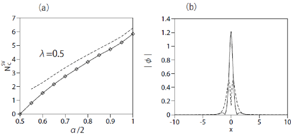
Figure 1: (a) The 2D SV solitons exist and are stable at norms below the critical value, $N_{\mathrm{c}}^{\mathrm{(SV)}}$, which is plotted vs. the half-LI, $\alpha/2$, for $\lambda=0.5$ and $\gamma=0$ in Eq. (4). The collapse takes place at $N>N_{\mathrm{c}}^{\mathrm{(SV)}}$. The numerical result and its VA-predicted counterpart are shown by the dashed line and chain of rhombuses, respectively. (b) Cross sections of profiles of $\left|\phi_{+}\right|$ and $\left|\phi_{-}\right|$ in the SV state (continuous and dashed lines, respectively) produced by the numerical solution of the linearized version of Eq. (LABEL:u2D) with $\alpha=1$ (see the text). Reproduced from H. Sakaguchi and B. A. Malomed, One- and two-dimensional solitons in spin-orbit-coupled Bose-Einstein condensates with fractional kinetic energy, J. Phys. B: At. Mol. Opt. Phys. 55, 155301 (2022) [see Ref. [37]], with the permission of IOP Publishing.

Figure 1(a) demonstrates that, as predicted by the VA and confirmed by numerical results, the fractional SOC system gives rise to stable SVs in the interval of LI values

$$1<\alpha\leq 2,$$ (27)

at norms below a critical value, $N\,<N_{\mathrm{c}}^{\mathrm{(SV)}}(\alpha)$, while at $N\,>N_{\mathrm{c}}^{\mathrm{(SV)}}(\alpha)$ the solitons are destroyed by the collapse, i.e., catastrophic self-compression of the field leading to the appearance of a singularity after a finite evolution time. The proximity of the VA-predicted and numerically found stability boundaries in Fig. 1(a) demonstrates that the VA, based on the simple ansatz (25), may produce reasonable results even for the complex system including the fractional diffraction (kinetic-energy operator), SOC, and the nonlinear interactions.

An exact property of the system is that $N_{\mathrm{c}}^{\mathrm{(SV)}}(\alpha=1)=0$, i.e., no SVs exist at $\alpha\leq 1$. In the case of $\alpha-1\rightarrow+0$, the SV exists with an infinitesimal amplitude, hence it can be found as a numerical solution of the linearized version of Eq. (LABEL:u2D) with $\alpha=1$. Cross-sections of components $\left|u_{\pm}\right|$ of the latter solution are displayed in Fig. 1(b). Actually, these plots adequately represent the shape of the SV solitons in the general case, when the nonlinearity is present.

The SV solitons are stable for $\gamma<1$ in Eqs. (LABEL:+-). For $\gamma>1$, the SVs are unstable, while in this case there are stable solitons in the form of mixed modes, which mix zero-vorticity terms and ones with vorticities $+1$ and $-1$, see further details in Ref. [37].

III The Emulation of the fractional Schrödinger equations (FSEs) in optics

III.1 Linear equations for the paraxial light propagation in optical systems emulating fractional diffraction

Realizations of the fractional quantum systems were proposed in solid-state settings, such as Levy crystals [46] and exciton-polariton condensates in semiconductor microcavities [47]. However, no experimental demonstration of the fractional quantum mechanics has been demonstrated thus far.

A more promising approach to the physical realization of FSEs in the form of classical equations is suggested by the commonly known similarity of the Schrödinger equation in quantum mechanics and the propagation equation for the amplitude of the classical optical field in the usual case of paraxial diffraction, with time $t$ replaced, as the evolution variable, by the propagation distance, $z$ [48]. A scheme for the realization of this possibility was proposed by Longhi in 2015 [49], who considered the transverse light dynamics in optical cavities with the $4f$ (four-focal-lengths) structure. As shown in Fig. 2, the proposed setup incorporates two lenses and a phase mask, which is placed in the middle (Fourier) plane. The lenses perform the direct and inverse Fourier transforms of the light beam with respect to the single or two transverse coordinates, thus implementing Eq. (10) or (13) and the inverse form of these equations. The Fourier decomposition splits the beam into spectral components with transverse wavenumbers $\left(p,q\right)$, the distance of each component from the optical axis being, roughly speaking,

$$R\sim\sqrt{p^{2}+q^{2}}$$ (28)

The action of the fractional diffraction in the Fourier space amounts, according to Eq. (9) or (14), to the local phase shift

$$\hat{\Psi}\left(p,q\right)\rightarrow\hat{\Psi}\left(p,q\right)\exp\left[i\left(p^{2}+q^{2}\right)^{\alpha}Z\right],$$ (29)

where $Z$ is the propagation distance which accounts for the fractional diffraction. The corresponding differential phase shift of the Fourier components is imposed by the phase mask in Fig. 2, which is designed so that the local shift introduced my the mask at distance $R$ from the axis emulates relation (29), with $R$ and $\left(p,q\right)$ related according to Eq. (28). In reality, the required mask, which is the central element of the setup, can be created as a computer-generated hologram [11]. Thus, the light beam recombined by the right lens in Fig. 2 carries the phase structure corresponding to the action of the fractional diffraction.

In addition to that, the curved mirror at the left edge of the cavity in Fig. 2 introduces (prior to the action of the Fourier decomposition) a phase shift which represents the action of potential $V\left(x,y\right)$ in Eq. (11). The layer of the gain medium placed next to the mirror in Fig. 2 may be used to amplify particular modes in the transverse structure of the light beam.

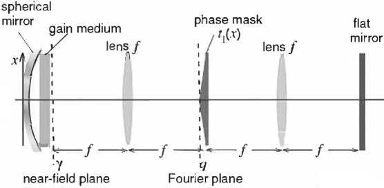
Figure 2: The setup proposed in Ref. [49] for the emulation of the FSE in the optical cavity. The left and right lenses perform, respectively, the spectral (Fourier) decomposition and recombination of the light beam with respect to the transverse coordinates. The phase mask placed in the central Fourier plane introduces the differential phase shift which emulates the fractional diffraction,as per Eqs. (28) and (29). The spherical mirror and gain medium at the left edge of the cavity introduce an effective potential. Reproduced with permission from S. Longhi, Fractional Schrödinger equation in optics, Opt. Lett. 40, 1117-1120 (2015) [see Ref. [49]]. Copyright 2015, Optica.

The setup which is outlined above provides a single-step transformation of the optical beam. The continuous FSE (11) is then introduced as an approximation for many cycles of circulation of light in the cavity, assuming that each cycle introduces a small phase shift (29). The 1D version of the FSE is obtained as the obvious reduction of the 2D scheme.

III.2 The emulation of the fractional diffraction in nonlinear optical systems: Fractional nonlinear Schrödinger equations (FNLSEs) in the spatial domain

III.2.1 The cubic nonlinearity in 1D

Once the FSE may be implemented as the propagation equation in optics under the action of the effective fractional diffraction, a natural possibility is to include the self-focusing nonlinearity of the optical material in the same system. The accordingly modified one-dimensional Eq. (8) is the fractional nonlinear Schrödinger equation (FNLSE),

$$i\frac{\partial\Psi}{\partial z}=\frac{1}{2}\left(-\frac{\partial^{2}}{\partial x^{2}}\right)^{\alpha/2}\Psi+V(x)\Psi-g|\Psi|^{2}\Psi,$$ (30)

where $g>0$ is the coefficient of the Kerr-nonlinearity coefficient, cf. FGPE (19). Then, steady-state solutions to Eq. (30), with real propagation constant $k$, are looked for as

$$\Psi(x,z)=\mathrm{exp}(ikz)U(x),$$ (31)

cf. Eq. (15), where real function $U(x)$ satisfies the equation

$$kU+\frac{1}{2}\left(-\frac{\partial^{2}}{\partial x^{2}}\right)^{\alpha/2}U+V(x)U-gU^{3}=0.$$ (32)

Localized solutions, i.e., fractional solitons, are characterized by their power (alias norm, cf. Eq. (23),

$$P=\int_{-\infty}^{+\infty}U^{2}(x)dx.$$ (33)

The stability of these states against small perturbations is investigated by looking for solutions in the form of

$$\Psi=\mathrm{exp}(ikz)[U(x)+a(x)\mathrm{exp}(\lambda z)+b^{\ast}(x)\mathrm{exp}(\lambda^{\ast}z)],$$ (34)

where $a(x)$ and $b^{\ast}(x)$ represent the perturbation, and $\lambda$, which may be complex, is the instability growth rate. Substituting expression (34) in Eq. (30), one derives linearized equations for the small perturbations,

$$i\lambda a = \frac{1}{2}\left(-\frac{\partial^{2}}{\partial x^{2}}\right)^{\alpha/2}a+ka+gU^{2}(x)(2a+b),$$

$$i\lambda b = -\frac{1}{2}\left(-\frac{\partial^{2}}{\partial x^{2}}\right)^{\alpha/2}b-kb-gU^{2}(x)(2b+a).$$ (35)

The stationary solution (31) is stable if all eigenvalues produced by the numerical solution of Eq. (35) have Re$(\lambda)=0$.

Straightforward analysis of Eq. (30) reveals a scaling relation between the soliton’s power and propagation constant:

$$P(k,g)=P_{0}(\alpha)g^{-1}k^{1-1/\alpha},$$ (36)

with some coefficient $P_{0}(\alpha)$. Relation (36) satisfies the necessary stability condition, viz., the celebrated Vakhitov-Kolokolov (VK) criterion, $dP/dk>0$ [50, 51] at $\alpha>1$, suggesting that the corresponding soliton family may be stable. The case of $\alpha=1$, which corresponds to $dP/dk=0$ in Eq. (36), implies the occurrence of the critical collapse, which makes all solitons unstable, similar to the family of Townes solitons produced by the 2D cubic nonlinear Schrödinger equation with the normal (non-fractional) diffraction ($\alpha=2$) [53, 51, 52]. For $\alpha<1$, relation (36) contradicts the VK criterion, yielding $dP/dk<0$, which implies strong instability of the solitons, driven by the supercritical collapse [51, 52].

Similar to what is outlined above for the system of FGPEs (LABEL:+-), approximate fractal-soliton solutions of FNLSE (32) can be sought for by means of VA [21, 54]. To this end, the Lagrangian of Eq. (32) is used (cf. Eq. (24)),

$$L=\frac{k}{2}\int_{-\infty}^{+\infty}dxU^{2}(x)+\frac{1}{4\pi}\int_{0}^{+\infty}dpp^{\alpha}\int\int d\xi dx\cos\left(p(x-\xi)\right)U(x)U(\xi)-\frac{g}{4}\int_{-\infty}^{+\infty}dxU^{4}(x).$$ (37)

The variational ansatz for the solitons can be adopted as the usual Gaussian with width $W$ and amplitude $A$ (cf. Eq. (25)),

$$U(x)=A\exp\left(-\frac{x^{2}}{2W^{2}}\right),$$ (38)

whose power (33) is

$$P=\sqrt{\pi}A^{2}W.$$ (39)

The substitution of ansatz (38) in Lagrangian (37) and integration yields the effective Lagrangian, in which the amplitude is eliminated in favor of the power by means of Eq. (39):

$$L_{\mathrm{eff}}=-\frac{\mu}{2}P+\frac{\Gamma\left(\left(1+\alpha\right)/2\right)}{4\sqrt{\pi}}\frac{P}{W^{\alpha}}-\frac{g}{4\sqrt{2\pi}}\frac{P^{2}}{W},$$ (40)

cf. Eq. (26).

Typical examples of the fractional solitons with the parameters predicted by the Euler-Lagrange equations, $\partial L_{\mathrm{eff}}/\partial P=\partial L_{\mathrm{eff}}/\partial W=0$, and their comparison to numerical solutions obtained for the same values of $\alpha$ and $k$ are displayed in Fig. 3. Further, the characteristic of the soliton family in the form of the $P(k)$ dependence, as predicted by the VA and produced by the numerical solution, is plotted in Fig. 4. These results demonstrate that VA provides reasonable accuracy.

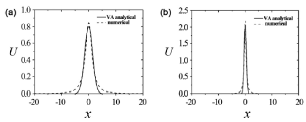
Figure 3: Fractional solitons with $k=0.3$ (a) and $2.0$ (b), as predicted by the VA based on ansatz  (38), and their counterparts provided by the numerical solution of Eq. (32), for $\alpha=1.5$ and $g=1$. Reproduced with permission from Y. Qiu, B. A. Malomed, D. Mihalache, X. Zhu, L. Zhang, and Y. He, Soliton dynamics in a fractional complex Ginzburg-Landau model, Chaos Solitons Fract. 131, 109471 (2020) [see Ref. [54]]. Copyright 2020, Elsevier.

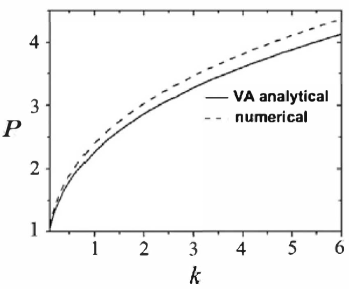
Figure 4: Power $P$ of the family of the fractional solitons vs. the propagation constant $k$, as predicted by the VA based on ansatz  (38), and provided by the numerical solution of Eq. (32), for $\alpha=1.5$ and $g=1$. Reproduced with permission from Y. Qiu, B. A. Malomed, D. Mihalache, X. Zhu, L. Zhang, and Y. He, Soliton dynamics in a fractional complex Ginzburg-Landau model, Chaos Solitons Fract. 131, 109471 (2020) [see Ref. [54]]. Copyright 2020, Elsevier.

An important result of the VA is the prediction of the fixed power for the quasi-Townes solitons at $\alpha=1$, for which, as said above, the critical collapse takes place [54]:

$$\left(P_{\mathrm{Townes}}\right)_{\mathrm{VA}}=\sqrt{2}\approx 1.41.$$ (41)

The numerically found counterpart of the VA prediction (41) is

$$\left(N_{\mathrm{Townes}}\right)_{\mathrm{num}}\approx 1.23.$$ (42)

Numerical investigation of the stability of the fractional-soliton family demonstrates that some of them may be weakly unstable at values of LI which are relatively far from $\alpha=2$. The instability does not destroy the solitons, leading to the onset of small-amplitude intrinsic oscillations in them [35].

III.2.2 Quadratic nonlinearity in 1D and 2D

In the case of quadratic (rather than cubic) self-focusing nonlinearity in the 1D space, the critical collapse takes place at $\alpha=1/2$, hence stable solitons may exist in the interval of $1/2<\alpha\leq 2$ [35], which is broader than its counterpart (27) in the case of the cubic self-focusing. In particular, the quadratic term may appear in Eq. (19) as $-\varepsilon|\psi|\psi$ with $\varepsilon>0$, representing a correction to the 1D FGPE induced by quantum fluctuations around the mean-field state [55].

In optics, the well-known quadratic nonlinearity appears in the system of coupled FNLEs for the second-harmonic-generation model:

$$i\frac{\partial\Psi_{1}}{\partial z} = \frac{1}{2}\left(-\frac{\partial^{2}}{\partial x^{2}}\right)^{\alpha/2}\Psi_{1}+\Psi_{1}^{\ast}\Psi_{2},$$

$$2i\frac{\partial\Psi_{2}}{\partial z} = \frac{1}{2}\left(-\frac{\partial^{2}}{\partial x^{2}}\right)^{\alpha/2}\Phi\Psi_{2}+Q\Psi_{2}+\frac{1}{2}\Psi_{1}^{2},$$

where $\Psi_{1}$ and $\Psi_{2}$ are amplitudes of the fundamental and second harmonics, and real $Q$ is the mismatch parameter, whose value may be fixed, by means of scaling, as$Q=$ $\pm 1$ or $0$.

Soliton solutions to Eq. (LABEL:uv), with real propagation constants $\beta$ and $2\beta$ of the fundamental-frequency and second-harmonic components, respectively, are looked for as

$$\Psi_{n}=\exp\left(in\beta z\right)\psi_{n}(x),~{}n=1,2,$$ (44)

where $\psi_{1,2}(x)$ are real localized profiles, see typical examples in Fig. 5. The existence and stability regions for solitons produced by system (LABEL:uv) in its parameter space were identified in Ref. [40]. In particular, the stability condition completely coincides with the above-mentioned VK criterion, $dP/d\beta>0$, applied to the system’s total power, $P(\beta)=\sum_{n=1,2}\int_{-\infty}^{+\infty}n^{2}\psi_{n}^{2}(x)dx$.

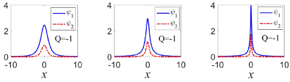
Figure 5: Examples of stable solitons produced by Eq. (44) with $\alpha=1.5$, $1.0$, and $0.7$ (the left, central, and right panels, respectively). In this case, $Q=-1$, and all the solitons correspond to $\beta=0.45$ in Eq. (44). The figure is borrowed from Ref. [40]. Reproduced from P. Li, H. Sakaguchi, L. Zeng, X. Zhu, D. Mihalache, and B. A. Malomed, Second-harmonic generation in the system with fractional diffraction, Chaos, Solitons & Fractals 173, 113701 (2023) [see Ref. [40]] with the permission of Elsevier Publishing.

In the 2D space, the cubic self-focusing nonlinearity gives rise to the critical collapse, as mentioned above, for $\alpha=2$, and to the supercritical collapse at all values of $\alpha<2$, therefore all the 2D fractional solitons are unstable. 2D solitons, including ones with embedded vorticity, may be stabilized in the model including the cubic self-focusing and quintic defocusing. As shown in Ref. [26], families of stable solitons produced by the 2D FNLSE with the cubic-quintic nonlinearity and $\alpha<2$ are qualitatively similar to their counterparts which were studied in detail in the 2D equation with the same nonlinearity and normal (non-fractional) diffraction, corresponding to $\alpha=2$ [57].

On the other hand, the 2D version of the second-harmonic-generating system based on Eq. (LABEL:uv) initiates the collapse only at $\alpha\leq 1$, while 2D solitons may be stable in the above-mentioned intervals (27). However, such solutions have not been investigated, as yet.

III.2.3 Fast moving modes in the fractional medium: reduction to the non-fractional equation

The definition of the Riesz derivative, given by Eq. (9), breaks the commonly known Galilean invariance of Eq. (30) with the non-fractional diffraction ($\alpha=2$), in the absence of the external potential ($V=0$). Nevertheless, the FNLSE (as well as the linear FSE) can be essentially simplified for fast moving modes (in the spatial domain the “moving” modes are actually ones tilted in the $\left(x,z\right)$ plane) [12]. To this end, one can consider solutions built as a product of a slowly varying amplitude $\psi(x)$ and a rapidly oscillating continuous-waver (CW) carrier with large wavenumber $\mathcal{P}$:

$$\Psi\left(x,z\right)=\psi(x,z)e^{i\mathcal{P}x},$$ (45)

The substitution of ansatz (45) in the nonlocally defined Riesz derivative in Eq. (9) leads to a quasi-local expression expanded in powers of small $1/\mathcal{P}$:

$$\left(-\frac{\partial^{2}}{\partial x^{2}}\right)^{\alpha/2}\left(\psi(x)e^{iPx}\right)=e^{iPx}|\mathcal{P}|^{\alpha}\left[\psi+\sum_{n=1}^{\infty}(-i)^{n}\frac{\alpha\left(\alpha-1\right)...\left(\alpha-n+1\right)}{n!P^{n}}\frac{\partial^{n}\psi}{\partial x^{n}}\right].$$ (46)

Next, the substitution of expansion (46), truncated at a finite order, $n=n_{\max}$, in Eq. (30) produces the local nonlinear Schrödinger equation with higher-order diffraction terms corresponding to $n\geq 3$ in Eq. (46). As concerns the convective term $\sim i\partial\psi/\partial x$, which corresponds to $n=1$ in Eq. (46), it may be eliminated by rewriting the resulting equation in the coordinate system moving (tilted) with the group velocity

$$V_{\mathrm{gr}}=\left(\alpha/2\right)|\mathcal{P}|^{\alpha-1}\mathrm{sgn}(\mathcal{P}),$$ (47)

i.e., replacing coordinate $x$ by $\tilde{x}\equiv x-V_{\mathrm{gr}}z$. Lastly, the term with $n=2$ in expansion (46) gives rise to the usual second-order diffraction term, with coefficient $D_{2}=(1/2)\alpha\left(\alpha-1\right)|\mathcal{P}|^{-\left(2-\alpha\right)}$. Thus, the resulting equation, truncated at $n_{\max}=2$, takes the form of the usual (non-fractional) nonlinear Schrödinger equation,

$$i\frac{\partial\tilde{\psi}}{\partial z}=-\frac{1}{2}D_{2}\frac{\partial^{2}\tilde{\psi}}{\partial\tilde{x}^{2}}-g\left|\tilde{\psi}\right|^{2}\tilde{\psi},$$ (48)

which gives rise to the commonly known solutions, such as solitons.

III.3 Systems of fractional nonlinear Schrödinger equations with the cubic nonlinearity

III.3.1 Fractional domain walls

Extension of the fractional model for copropagating optical waves with orthogonal polarizations or different carrier wavelength is a natural possibility, which was addressed in Ref. [36] for the case of the self-defocusing cubic nonlinearity. The corresponding 1D system of coupled FNLSEs for wave amplitudes $\Psi$ and $\Phi$ is

$$i\frac{\partial\Psi}{\partial z} = \frac{1}{2}\left(-\frac{\partial^{2}}{\partial x^{2}}\right)^{\alpha/2}\Psi+(|\Psi|^{2}+\beta|\Phi|^{2})\Psi-\lambda\Phi,$$

$$i\frac{\partial\Phi}{\partial z} = \frac{1}{2}\left(-\frac{\partial^{2}}{\partial x^{2}}\right)^{\alpha/2}\Phi+(|\Phi|^{2}+\beta|\Psi|^{2})v-\lambda\Psi,$$

where $\beta>0$ is the relative strength of the cross-phase-modulation (XPM) interaction, while the coefficient of the self-phase modulation is scaled to be $1$. In the case of orthogonal polarizations, natural XPM values are $\beta=2/3$ or $2$, for the linear and circular polarizations, respectively. The copropagation of optical waves carried by different wavelengths is governed by the same system (LABEL:PsiPhi) with $\beta=2$ [48]. Other positive values of $\beta$ are possible in photonic crystals [48].

In addition to XPM, the two components may be coupled in Eq. (LABEL:PsiPhi) by linear terms with real coefficient $\lambda$. The linear coupling accounts for the twist of the waveguide in the case of the copropagation of linear polarizations, or elliptic deformation of the waveguide in the case of circular polarizations [48].

As usual, stationary states with a real propagation constant $k$ are looked for as $\left\{\Psi,\Phi\right\}=\exp\left(ikz\right)\left\{U(x),V(x)\right\}$, where real real functions $U(x)$ and $V(x)$ are solutions of the system

$$kU+\frac{1}{2}\left(-\frac{\partial^{2}}{\partial x^{2}}\right)^{\alpha/2}U+(U^{2}+\beta V^{2})U-\lambda V = 0,$$

$$kV+\frac{1}{2}\left(-\frac{\partial^{2}}{\partial x^{2}}\right)^{\alpha/2}V+(V^{2}+\beta U^{2})V-\lambda U = 0.$$

Natural patterns supported by Eq. (LABEL:UV) with $k<0$ are optical domain walls (DWs) [58, 59, 60], which link different CW states at $x\rightarrow\pm\infty$, that are mirror images to each other:

$$\left\{\begin{array}[]{c}U(x\rightarrow\pm\infty)\\ V(x\rightarrow\pm\infty)\end{array}\right\}=\frac{1}{\sqrt{2}}\left\{\begin{array}[]{c}\sqrt{-\frac{k}{2}+\frac{\lambda}{\beta-1}}\pm\sqrt{-\frac{k}{2}-\frac{\lambda}{\beta-1}}\\ \sqrt{-\frac{k}{2}+\frac{\lambda}{\beta-1}}\mp\sqrt{-\frac{k}{2}-\frac{\lambda}{\beta-1}}\end{array}\right\},$$ (51)

with equal total power densities: $U^{2}(x\rightarrow\pm\infty)+V^{2}(x\rightarrow\pm\infty)=-k$. In particular, in the absence of the linear coupling, $\lambda=0$, $U(x)$ and $V(x)$ vanish at $x\rightarrow+\infty$ and $-\infty$, respectively. The asymmetric CW states (51) exist under the condition of the immiscibility [61] of the two components:

$$\beta-1>\left(\beta-1\right)_{\mathrm{immisc}}\equiv 2\lambda/|k|.$$ (52)

In the case of $\beta=3$ (which plays a special role in various systems, making it possible to find exact DW solutions [62, 60]), substitution $\left\{U(x),V(x)\right\}=(1/2)\left[\sqrt{\lambda-k}\mp W(x)\right]$ reduces two equations (LABEL:UV) to a single one,

$$(k+\lambda)W+\frac{1}{2}\left(-\frac{\partial^{2}}{\partial x^{2}}\right)^{\alpha/2}W+W^{3}=0.$$ (53)

In this case, the boundary conditions (51) which determined the DW solutions reduce to

$$\lim_{x\rightarrow\pm\infty}W(x)=\pm(1/2)\sqrt{-k-\lambda}.$$ (54)

Note that it follows from Eq. (52) with $\beta=3$ that $\sqrt{-k-\lambda}$ is real, hence the boundary conditions (54) make sense.

The DW states produced by Eq. (LABEL:PsiPhi) are stable (in particular, the CW background states at $x\rightarrow\pm\infty$ are not subject to modulational instability). A set of numerically obtained DW solutions are displayed in Fig. 6.

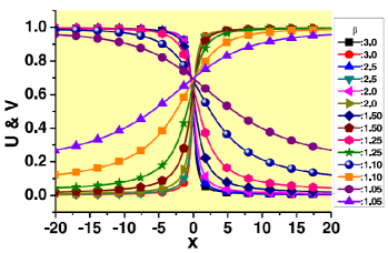
Figure 6: A set of stable DW patterns with $k=-1$, produced by the numerical solution of Eq. (LABEL:UV) in the absence of the linear coupling ($\lambda=0$), with LI $\alpha=1$, and different values of the XPM coefficient $\beta$ indicated in the figure. Reproduced from S. Kumar, P. Li, and B. A. Malomed, Domain walls in fractional media, Phys. Rev. E 106, 054207 (2022) [see Ref. [36]] with the permission of AIP Publishing.

A more general bimodal system, with different values of LI in its coupled components, $\alpha_{1}$ and $\alpha_{2}$, was considered too [36]. It also gives rise to families of stable DW patterns, which, unlike those displayed in Fig. 6, are spatially asymmetric with respect to the midpoint.

III.3.2 Couplers and spontaneous symmetry breaking

Another model which naturally gives rise to a system of coupled FNLSEs with the fractional diffraction and cubic self-focusing acting in each equation, and linear coupling between the equations, introduces a dual-core optical waveguide [34, 38]:

$$i\frac{\partial\Psi_{1}}{\partial z} = \frac{1}{2}\left(-\frac{\partial^{2}}{\partial x^{2}}\right)^{\alpha/2}\Psi_{1}-|\Psi_{1}|^{2}\Psi_{1}-\Psi_{2},$$

$$i\frac{\partial\Psi_{2}}{\partial z} = \frac{1}{2}\left(-\frac{\partial^{2}}{\partial x^{2}}\right)^{\alpha/2}\Psi_{2}-|\Psi_{2}|^{2}\Psi_{2}-\Psi_{1},$$

where the coefficient of the linear coupling is scaled to be $1$ (cf. coefficient $\lambda$ in Eq. (LABEL:PsiPhi)). As well as the single FNLSE (30), system (LABEL:coupler) is meaningful in the interval of LI index given by Eq. (27), when the collapse does not take place.

Steady-state solutions to Eq. (LABEL:coupler) with real propagation constant $k>0$ are looked for $\Psi_{1,2}=\exp\left(ikz\right)U_{1,2}(x)$, where real functions $U_{1,2}(x)$ satisfy equations

$$kU_{1}+\frac{1}{2}\left(-\frac{d^{2}}{dx^{2}}\right)^{\alpha/2}U_{1}-U_{1}^{3}-U_{2},$$

(56)

$$kU_{2}+\frac{1}{2}\left(-\frac{d^{2}}{dx^{2}}\right)^{\alpha/2}U_{2}-U_{2}^{3}-U_{1},$$

Two-component solitons produced by Eq. (LABEL:coupler) are characterized by the total power,

$$P=\int_{-\infty}^{+\infty}\left[U_{1}^{2}(x)+U_{2}^{2}(x)\right]dx.$$ (57)

In the case of the normal (non-fractional) diffraction, $\alpha=2$, a fundamental property of the two-component solitons is spontaneous symmetry breaking (SSB), which destabilizes the obvious symmetric solitons, with $U_{1}(x)=U_{2}(x)$, at a critical value of the soliton’s power, $P=P_{\mathrm{cr}}$, and replaces the unstable symmetric modes by asymmetric ones, with $U_{1}(x)\neq U_{2}(x)$. The asymmetry of the solitons is naturally quantified by the normalized difference in powers of their components, i.e.,

$$\Theta\equiv P^{-1}\int_{-\infty}^{+\infty}\left((U_{1}^{2}(x)-U_{2}^{2}(x)\right)dx.$$ (58)

The SSB phenomenology for solitons was studied in detail theoretically [63]-[68], and was recently demonstrated experimentally in dual-core optical fibers [69] with the second-order (non-fractional) GVD. A characteristic peculiarity of the SSB in this system is that the transition from the symmetric solitons to asymmetric ones is performed through a subcritical bifurcation [70] (similar to a symmetry-breaking phase transition of the first kind), which means that a stable asymmetric soliton solution emerges at a value of $P$ which is slightly smaller than $P_{\mathrm{cr}}$, i.e., in the subcritical range. In this case, the branch of the asymmetric soliton states, appearing at $P=P_{\mathrm{cr}}$, originally moves in the backward direction, being unstable (therefore, another name of this bifurcation is the backward one). Then, this branch turns forward, getting stable, at the turning point (see, e.g., the left panel of Fig. 7).

The system of equations (56), with the fractional Riesz derivative, defined as per Eq. (9), can be derived from the Lagrangian,

$$L=\int_{-\infty}^{+\infty}\left[\frac{k}{2}\left(U_{1}^{2}+U_{2}^{2}\right)\right]dx+H,$$ (59)

where the Hamiltonian is

$$H=\int_{-\infty}^{+\infty}\left\{-\frac{1}{4}\left[U_{1}^{4}(x)+U_{2}^{4}(x)\right]-U_{1}(x)U_{2}(x)\right\}dx$$

$$+\frac{1}{4\pi}\int_{0}^{+\infty}p^{\alpha}dp\int_{-\infty}^{+\infty}dx\int_{-\infty}^{+\infty}dx^{\prime}\cos\left(p\left(x-x^{\prime}\right)\right)\left[U_{1}(x)U_{1}(x^{\prime})+U_{2}(x)U_{2}(x^{\prime})\right],$$ (60)

cf. Eq. (37). Using the Lagrangian, VA can be applied to the system. An appropriate tractable ansatz, with width $W$, power $P$, and angle $\chi$ accounting for the norm distribution between the components, is

$$U_{1}(x)=\sqrt{\frac{P}{2W}}\left(\cos\chi\right)\mathrm{sech}\left(\frac{x}{W}\right),U_{2}(x)=\sqrt{\frac{P}{2W}}\left(\sin\chi\right)\mathrm{sech}\left(\frac{x}{W}\right).$$ (61)

In terms of this ansatz, the asymmetry parameter (58) is

$$\Theta_{\mathrm{VA}}=\cos\left(2\chi\right)\equiv\sqrt{1-S^{2}},S\equiv\sin\left(2\chi\right).$$ (62)

The calculation of Lagrangian (59) with ansatz (61) yields

$$L_{\mathrm{eff}}=\frac{P}{2}\left[k-\frac{P}{6W}\left(1-\frac{1}{2}S^{2}\right)-S+\left(1-2^{1-\alpha}\right)\Gamma(1+\alpha)\frac{\zeta(\alpha)}{(\pi W)^{\alpha}}\right]$$ (63)

(cf. Eq. (40)), where $\Gamma$ and $\zeta$ are the Gamma- and zeta-functions. The effective Lagrangian (63) gives rise to the Euler-Lagrange equations, $\partial L_{\mathrm{eff}}/\partial W=\partial L_{\mathrm{eff}}/\partial\left(\sin(2\chi\right))=0$, which amount to relation $W=PS/6$ and an equation for parameter $S$ (which is defined in Eq. (62)),

$$S^{\alpha-1}\left(1-\frac{S^{2}}{2}\right)=\frac{\alpha}{\pi^{\alpha}}\left(1-2^{1-\alpha}\right)\Gamma(1+\alpha)\zeta(\alpha)\left(\frac{6}{P}\right)^{\alpha}.$$ (64)

The SSB point, as which the family of the asymmetric solitons branches off from the symmetric one, corresponds to setting $S=1$ (which represents the symmetric soliton) in Eq. (64), the result being

$$\left(P_{\mathrm{SSB}}\right)(\alpha)=\frac{6}{\pi}\left[2\alpha\left(1-2^{1-\alpha}\right)\Gamma(1+\alpha)\zeta(\alpha)\right]^{1/\alpha}.$$ (65)

In the case of $\alpha=2$, Eq. (65) reproduces the known result produced by the VA for the non-fractional coupler, viz., $\left(P_{\mathrm{SSB}}\right)(\alpha=2)=2\sqrt{6}\approx 4.899$ [67, 68]. Note that the SSB point for the usual coupler is known in an exact form, which can be found without the use of VA [63],

$$\left(P_{\mathrm{SSB}}\right)_{\mathrm{exact}}(\alpha=2)=8/\sqrt{3}\approx 4.619,$$ (66)

i.e., the relative error of the VA prediction is $\approx 5.7\%$. In the opposite limit of $\alpha-1\rightarrow+0$, Eq. (65) gives the respective VA result as $\left(P_{\mathrm{SSB}}\right)\left(\alpha\rightarrow 1\right)=(12/\pi)\ln 2\approx 2.648$.

Eventually, the VA predicts the basic characteristic of the system, viz., the dependence of the asymmetry parameter (58) on the power, $\Theta(P)$, in an implicit form [38]:

$$\left(1-\Theta_{\mathrm{VA}}^{2}\right)^{(\alpha-1)/2}\left(1+\Theta_{\mathrm{VA}}^{2}\right)=\frac{2\alpha}{\pi^{\alpha}}\left(1-2^{1-\alpha}\right)\Gamma(1+\alpha)\zeta(\alpha)\left(\frac{6}{P}\right)^{\alpha}.$$ (67)

In the limit of $\alpha\rightarrow 1$, this relation yields

$$\Theta_{\mathrm{VA}}(P;\alpha\rightarrow 1)=\sqrt{\frac{12\ln 2}{\pi P}-1}.$$ (68)

The VA predictions following from Eqs. (67) and (65) for different values of LI $\alpha$ are plotted in Fig. 7, along with results produced by the numerical solution of Eq. (56). It is observed that the subcritical character of the SSB bifurcation becomes more pronounced with the decrease of $\alpha$. In the limit of $\alpha=1$, the dependence is available solely in the VA form, given by Eq. (68), while the numerical solutions were obtained only for $\alpha\geq 1.2$ [38]. The VA-predicted $\Theta(P)$ dependence for $\alpha=1$, given by Eq. (68), takes the extreme subcritical form (defined as per Ref. ([39]), in which the branch of the asymmetric solitons, going backward from the SSB point, never turns forward, always remaining unstable). The dependence (68) terminates at point $\Theta=1$, i.e., at $P=(6/\pi)\ln 2\approx\allowbreak 1.\allowbreak 324$ (see the left panel in Fig. 7), as definition (58) does not admit values $|\Theta|>1$.

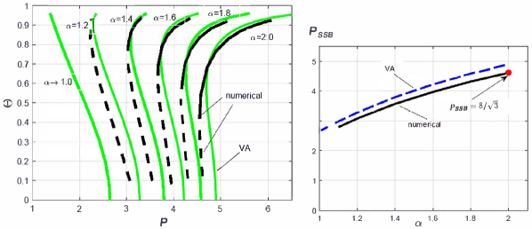
Figure 7: Left: A set of dependences of the soliton’s asymmetry parameter (58) on total power (57), as predicted by the VA through Eq. (67), and as produced by the numerical solution of Eq. (56), for different values of LI $\alpha$. Right: the value of the soliton’s power at the SSB bifurcation point vs. the LI, as predicted by the VA, and as found from the numerical solution. The red circle at the end of the numerical curve represents the known exact value (66) for $\alpha=2$ (the usual system with the non-fractional diffraction). Reproduced from D. V. Strunin and B. A. Malomed, Symmetry-breaking transitions in quiescent and moving solitons in fractional couplers, Phys. Rev. E 107, 064203 (2023) [see Ref. [38]] with the permission of AIP Publishing.

In addition to that, Fig. 8 displays a set of numerically generated dependences $P(k)$ for different fixed values of LI. The SSB points are those separating stable and unstable segments of the symmetric-soliton branches, from which ones representing unstable asymmetric solitons stem. The stability boundaries, observed on the asymmetric branches for $\alpha=2.0,1.8,1.6,$ and $1.4$, correspond to the above-mentioned turning points, while the branches for $\alpha=1.2$ and $1.1$ do not reach those points, therefore they seem completely unstable in Fig. 8.

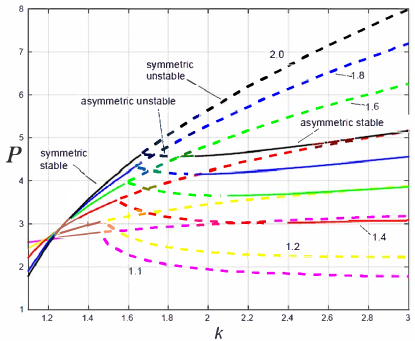
Figure 8: Dependences between the total power, $P$, and the propagation constant, $k$, for families of symmetric and asymmetric solitons produced by the numerical solution of Eqs. (LABEL:coupler) and (56), for different fixed values of LI $\alpha$. Solid and dashed segments of the curves represent, respectively, stable and unstable parts of the soliton families. Reproduced from D. V. Strunin and B. A. Malomed, Symmetry-breaking transitions in quiescent and moving solitons in fractional couplers, Phys. Rev. E 107, 064203 (2023) [see Ref. [38]] with the permission of AIP Publishing.

The analysis of the SSB phenomenology was also developed for moving (tilted) two-component solitons (recall it is a nontrivial extension of the analysis because the fractional diffraction breaks the system’s Galilean invariance), demonstrating that the symmetry-breaking bifurcation keeps its subcritical character, and values of the power at the bifurcation point become lower than for the quiescent solitons [38]. Collisions between moving solitons were studied too, with a conclusion that the collisions with small relative velocities lead to elastic rebound, which is followed by strongly inelastic symmetry-breaking interactions at intermediate values of the velocities, and, eventually, by restoration of the elasticity in collisions between fast solitons [38].

The analysis of SSB in solitons was also developed for the single-component FNLSE (30) with a symmetric double-well potential $V(x)$ [33]. On the contrary to what is shown here, in that case, the SSB bifurcation is of the supercritical (forward) type (i.e., it represents a symmetry-breaking phase transition of the second type). Furthermore, the same FNLSE with the self-defocusing nonlinearity ($g<0$ in Eq. (30)) does not break the symmetry of the ground state trapped by the double-well potential, but the increase of $|g|$ leads to spontaneous breaking of the antisymmetry of the first excited state trapped by the same potential.

IV The fractional group-velocity dispersion (GVD) in fiber cavities: The fractional Schrödinger equation in the temporal domain, and its experimental realization

Thus far, no experimental realization of the effective fractional diffraction for light beams in the spatial domain has been reported. Another option for the implementation of the concept of the fractional propagation in optics is to resort to the transmission of light pulses in the temporal domain, i.e., in fiber-based setups, with an effective fractional GVD. This option has been realized recently [11], thus providing the first experimental implementation of a fractional medium in any physical setting.

Confining the consideration to the linear propagation regime, the effective FSE for the optical amplitude $\Psi\left(\tau,z\right)$ in the temporal domain is written as

$$i\frac{{\partial\Psi}}{{\partial z}}=\left[{\frac{D}{2}{{\left({-\frac{{\partial^{2}}}{{\partial{\tau^{2}}}}}\right)}^{\alpha/2}}-\sum\limits_{k=2,3...}{\frac{{\beta_{k}}}{{k!}}{{\left({i\frac{\partial}{{\partial\tau}}}\right)}^{k}}}}\right]\Psi,$$ (69)

where the evolutional variable is the propagation distance $z$, and the effective coordinate is the reduced time [48], $\tau=t-z/V_{\mathrm{gr}}$, where $V_{\mathrm{gr}}$ is the group velocity of the carrier wave. In this equation, the fractional GVD is determined by LI $\alpha$ (cf. Eq. (8)), $D$ is the corresponding coefficient, and the usual derivatives represent the second- and higher-order GVD, for $k=2$ and $k\geq 3$, respectively, which act in the setup along with the fractional GVD.

The solution of Eq. (69) can be easily written for the Fourier transform of the optical field,

$$\hat{\Psi}\left(\omega,z\right)=\int_{-\infty}^{+\infty}\exp\left(i\omega\tau\right)\Psi\left(\tau,z\right)d\omega$$ (70)

(cf. Eq. (10)), as

$$\hat{\Psi}(\omega,z)=\exp\left({-i\left({\frac{D}{2}|\omega{|^{\alpha}}-\sum\limits_{k=2,3,...}{\frac{{\beta_{k}}}{{k!}}}{\omega^{k}}}\right)z}\right)\hat{\Psi}_{\mathrm{input}}(\omega),$$ (71)

where $\hat{\Psi}_{\mathrm{input}}(\omega)$ is the Fourier transform of initial condition, i.e., the optical signal coupled into the fiber at $z=0$.

The fiber-cavity setup which was used for the experimental emulation of the fractional GVD is displayed in Fig. 9. It incorporates two holograms, with the left one shaping the input pulse. The second hologram, installed at the central position, was designed as the element similar to the phase mask in the setup presented above in Fig. 2 (it is displayed in the rotated form, to make its internal structure visible). It imposes the differential phase shift onto spectral components of the light signal, simulating the action of the fractional GVD as per Eq. (71) (cf. Eq. (29)).

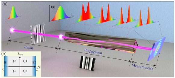
Figure 9: (a) The setup elaborated in Ref. [11] for the realization of the fractional GVD in the fiber-laser cavity. The hologram installed in the initial section is employed to shape the input pulse. In the propagation section, the second hologram plays the role of the phase mask (cf. Fig. 2), which imposes the differential phase shift onto spectral components of the light signal, to emulate the effect of the fractional GVD. This hologram is shown in the rotated position, to display its structure. The initial temporal profile of the pulse belonging to quadrant Q3 in (b), and its evolution in the propagation section are shown in the top of the panel. (b) Four different quadrants in the parameter plane ($L_{\mathrm{GVD}},\alpha$). Q1 and Q2 correspond to the cases of $L_{\mathrm{GVD}}>0$ with $1\leq\alpha\leq 2$ and $0\leq\alpha\leq 1$, respectively. Q3 and Q4 are defined similarly for $L_{\mathrm{GVD}}<0$. Areas B1 and B2 designate narrow strips with $\alpha$ close to $0$ or $2$, respectively. Reproduced with permission from S. Liu, Y. Zhang, B. A. Malomed, and E. Karimi, Experimental realisations of the fractional Schrödinger equation in the temporal domain, Nature Comm. 14, 222 (2023) [see Ref. [11]]. Copyright 2023, Springer-Nature.

Experimental findings were compared with the theoretical result provided by Eq. (71), keeping only the second-order GVD $\sim\beta$, in addition to the fractional GVD [11]. Typical values of the dispersion coefficients in Eq. (71) are

$$D=21\times 10^{-3}\text{ ps}^{\alpha}\text{/m},\beta_{2}=-21\times 10^{-3}~{}\text{ps}^{2}\text{/m,}$$ (72)

where $\beta_{2}<0$ implies that it represents the anomalous second-order GVD [48], although the case of the normal GVD, corresponding to $\beta_{2}>0$, was considered too. The results were summarized as functions of two control parameters, namely, LI $\alpha$ and effective GVD length $L_{\mathrm{GVD}}$ (which corresponds to $z$ in Eq. (71)). The plane of these parameters is schematically defined in the inset to Fig. 9, where $\alpha$ varies from $0$ to $2$, while positive and negative values of $L_{\mathrm{GVD}}$ correspond to the anomalous and normal second-order GVD.

Basic experimental and theoretical results are reported in Fig. 10 for four characteristic cases, with parameters

$$(L_{\mathrm{GVD}},\alpha)=(5,1.25),(5,0.25),(-5,0.25),(-5,1.25),$$ (73)

that pertain, respectively, to quadrants Q1 – Q4 in Fig. 9(b). In Q1, the setup demonstrates competition between the splitting effect of the fractional GVD and the confining (anti-splitting) action of the anomalous second-order GVD. The competition maintains balance over a short propagation distance, $\simeq 40$ m. Then, the splitting effect becomes the dominant one, leading to fission of the pulse in two secondary ones. In Q2, small $\alpha=0.25$ implies that the fractional GVD is weak. Then, the dominant anomalous second-order GVD drives fragmentation of the input into a multi-jet pattern, which, however, stays confined, following the confining effect of the same GVD term observed at the initial stage of the evolution in Q1. In panel Q3, the fractional GVD remains weak, with the same value of LI, $\alpha=0.25$, as in Q2, while the second-order GVD flips its sign from anomalous to normal, leading to the fast split of the pulse in two. Finally, in quadrant Q4 the same normal second-order GVD as in Q3 cooperates with the strong fractional-GVD term ($\alpha=1.25$), producing extremely fast fission of the pulse in two fragments (note the difference by an order of magnitude between scales on the vertical axes in panels Q3 and Q4). Another difference between the relatively gentle splitting in Q3, driven by the normal second-order GVD, and more violent splitting in Q4, driven jointly by the second-order and fractional GVD terms, is that, in the latter case, the emerging fragments are loosely bound pulses, unlike tightly bound ones in Q3.

The dynamics displayed in Fig. 10 is reversible, therefore examples of the splitting, such as ones exhibited in panels Q1 and Q3, imply the possibility of fusion of colliding pulses into a single one, if the propagation distance $z$ varies in the opposite direction.

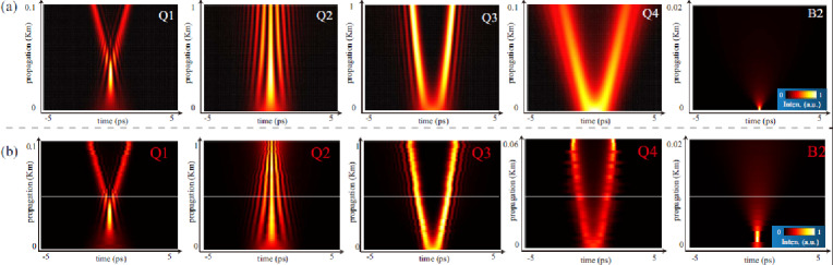
Figure 10: Different outcomes of the propagation of input light pulses in parameter regions Q1 – Q4 and B2, defined as per Fig. 9(b), are displayed in the plane of the temporal coordinate $\tau$ and propagation distance $z$, see Eq. (69). The color code represents local intensities of the pulses. Exact values of the parameters corresponding to Q1 – Q4 are fixed in Eq. (73), while B2 corresponds to $L_{\mathrm{GVD}}=0$ and $\alpha=2$. In all the cases, the dispersion parameters are fixed as per Eq. (72). Rows of panels (a) and (b) represent, severally, theoretical and experimental results. Note the great difference in the scales of the vertical axes ($z$) in panels Q2, Q3 ($z_{\max}=1$ km), Q1, Q4 ($z_{\max}=0.1$ km) and B2 ($z_{\max}=0.02$ km). Reproduced with permission from S. Liu, Y. Zhang, B. A. Malomed, and E. Karimi, Experimental realisations of the fractional Schrödinger equation in the temporal domain, Nature Comm. 14, 222 (2023) [see Ref. [11]]. Copyright 2023, Springer-Nature.

For the comparison’s sake, panels B2 in Fig. 10 demonstrate that, unlike the setup including the fractional GVD, the usual one, with $L_{\mathrm{GVD}}=0$ and $\alpha=2$ (see area B2 in the inset in Fig. 9(b)), very quickly leads to full destruction of the input pulse (note that largest propagation distance in panels B2 is $0.02$ km). Thus, the fractional GVD makes the outcome of the light propagation in the fiber cavity much more nontrivial.

A remarkable fact is close proximity between the experimental findings and the corresponding theoretical results, which are presented, respectively, in rows (b) and (a) of Fig. 10. In addition to that, Fig. 11 reports a set of theoretical results for the same dispersion parameters as in Eq. (72), but with another value of the LI, $\alpha=1$. In particular, Fig. 11(a) demonstrates that, under the action of fractional-only GVD ($L_{\mathrm{GVD}}=0$), the evolution of the input is generally similar to that in the case when the usual second-order GVD is present too, but the fractional term is the dominant one (case Q1 in Fig. 10): the input pulse quickly splits in a pair of secondary ones. Such a setting with the purely fractional GVD was not realized experimentally, as the usual GVD cannot be eliminated in the real setup. Further, if strong anomalous or normal second-order GVD is included, corresponding to $L_{\mathrm{GVD}}=+10$ and $-10$ in Figs. 11(b) and (c), respectively, the outcomes are also akin to what is shown for similar cases in panels Q2 and Q4 of Fig. 10: the fragmentation of the input into a non-expanding multi-jet pattern in the former case, or violent fission of the input in two loosely bound pulses in the latter case.

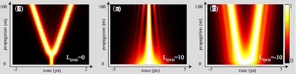
Figure 11: Different outcomes of the propagation of the input pulses, as predicted by simulations of the model based on Eq. (71) with the GVD parameters fixed as per Eq. (72), LI $\alpha=1$, and values of $L_{\mathrm{GVD}}$ indicated in panels (a,b,c), are displayed in the plane of $(\tau,z)$. The color code represents local intensities. Reproduced with permission from S. Liu, Y. Zhang, B. A. Malomed, and E. Karimi, Experimental realisations of the fractional Schrödinger equation in the temporal domain, Nature Comm. 14, 222 (2023) [see Ref. [11]]. Copyright 2023, Springer-Nature.

The experiments reported in Ref. [11] were also performed for the input pulse with the phase including a cubic term, $\sim\tau^{3}$. It is well known that, in the framework of the usual linear Schrödinger equation with the second-order GVD, this term initiated the propagation of a self-accelerating self-bending Airy wave [71, 72]. In the interval of LI values $1\leq\alpha\leq 1.80$, the results reported in Ref. [11] (not shown here in detail) demonstrate splitting of the input into a self-bending quasi-Airy wave and an additional one propagating along a straight trajectory.

All the experimental results demonstrating the implementation of the effective fractional GVD, summarized above and reported in detail in Ref. [11], have been obtained in the linear regime. The interplay of the strongly fractional GVD, with LI values $\alpha=1$ and $\alpha=0.2$, and the fiber’s self-focusing nonlinearity is a subject of a very recent experimental work [82]. In particular, it demonstrates spectral bifurcations of ultrashort optical pulses in the fiber-laser cavity, in the form of spontaneous transitions between the pulses with single- and multi-lobe structures.

V Conclusion

This aim of this paper is to present a concise summary of dynamical models of 1D and 2D media with fractional diffraction or dispersion, both linear and nonlinear ones. Two well-substantiated physical models of this type are fractional quantum mechanics for particles which, at the classical level, move by random Lévy flights [13, 14, 15], and the emulation of the effective fractional diffraction in optical cavities [49]. These models include the Riesz fractional derivatives [10] or the respective 2D fractional Laplacian, which are defined as per Eqs. (9) and (14). The Riesz derivative with LI (Lévy index) $\alpha$ amounts to the multiplication of the Fourier transform of the underlying wave field, $\hat{\Psi}(p)$, by $|p|^{\alpha}$. Equations (9) and (14) demonstrate that the Riesz derivatives and their 2D counterparts are represented, in the explicit form, not by differential operators, but rather by nonlocal integral ones.

The paper presents basic types of solitons produced by the nonlinear fractional models in a brief form, without an objective to produce a systematic review of the solitons in fractional systems. The absolute majority of theoretical results for the fractional solitons have been obtained by means of numerical methods. Nevertheless, the present review includes some quasi-analytical results based on the VA (variational approximation). Actually, the comparison with numerical findings demonstrates that the VA works surprisingly well too in these relatively complex nonlinear nonlocal models.

In addition to the theoretical results, the article includes a summary of the recently reported first experimental realization of the fractional optics. It is based on the fiber-cavity setup, in which the effective fractional GVD (group-velocity dispersion) is implemented by means of a specially designed phase plate (computer-generated hologram) [11].

There are essential topics dealing with the dynamics of fractional media which are not considered in this paper, which is not designed as a comprehensive review. One of such topics is the dynamics of fractional discrete systems. [73, 74, 75]. Others, which have attracted much interest recently (and may be relevant subjects for a more extensive review), are dissipative solitons and self-trapped vortices in models based on fractional complex Ginzburg-Landau equations [76, 77, 78, 54], as well as solitons in fractional parity-time-symmetric systems [79, 80, 81].

There are many possibilities for further theoretical and, especially, experimental developments in this area. In particular, on the theoretical side, a challenging objective (which is mentioned in this paper) is to derive equations of the FGPE (fractional Gross-Pitaevskii equation) type for a BEC (Bose-Einstein condensate) of quantum particles which are individually governed by the fractional Schrödinger equation. On the experimental side, obvious objectives are to realize the fractional diffraction in spatial-domain optics, and to create the predicted fractional solitons in such settings.

References

- [1] P. Clavin and G. Searby, Combustion Waves and Fronts in Flows (Cambridge University Press, Cambridge, UK, 2016).
- [2] A. P. Aldushin, B. A. Malomed, and Ya. B. Zeldovich, Phenomenological theory of spin combustion, Combustion and Flame 42, 1-6 (1981).
- [3] N. H. Abel, Oplösning af et Par Opgaver ved Hjelp af bestemte Integraler, Magazin for Naturvidenskaberne. Kristiania (Oslo), pp. 55–68 (1823).
- [4] M. Jeng, S.-L.-Y. Xu, E. Hawkins, and J. M. Schwarz, On the nonlocality of the fractional Schrödinger equation, J. Math. Phys. 51, 062102 (2010).
- [5] A. I. Saichev and G. M. Zaslavsky, Fractional kinetic equations: solutions and applications, Chaos 7, 753-764 (1997).
- [6] G. M. Zaslavsky, Chaos, fractional kinetics, and anomalous transport, Phys. Rep. 371, 461-580 (2002).
- [7] J. Liouville, Mémoire sur quelques questions de géométrie et de mécanique, et sur un nouveau genre de calcul pour résoudre ces questions, Journal de l’École Polytechnique Paris 13, 1–69 (1832).
- [8] V. V. Uchaikin, Fractional Derivatives for Physicists and Engineers (Springer, New York, 2013).
- [9] M. Caputo, Linear model of dissipation whose Q is almost frequency independent. II, Geophysical Journal International 13, 529–539 (1967).
- [10] M. Cai and C. P. Li, On Riesz derivative, Fractional Calculus and Applied Analysis 22, 287-301 (2019).
- [11] S. Liu, Y. Zhang, B. A. Malomed, and E. Karimi, Experimental realisations of the fractional Schrödinger equation in the temporal domain, Nature Comm. 14, 222 (2023).
- [12] B. A. Malomed, Optical solitons and vortices in fractional media: A mini-review of recent results, Photonics 8, 353 (2021).
- [13] N. Laskin, Fractional quantum mechanics and Lévy path integrals. Phys. Lett. A 268, 298-305 (2000).
- [14] N. Laskin, Fractional quantum mechanics (World Scientific: Singapore, 2018).
- [15] X. Guo and M. Xu, Some physical applications of fractional Schrödinger equation, J. Math. Phys. 47, 082104 (2006).
- [16] B. B. Mandelbrot, The Fractal Geometry of Nature (W. H. Freeman, New York, 1982).
- [17] S. Albeverio, R. Hoegh-Krohn, and S. Mazzucchi, Mathematical Theory of Feynman Path Integrals : An Introduction (Springer, Berlin and Heidelberg, 2008).
- [18] C. Klein, C. Sparber, and P. Markowich, Numerical study of fractional nonlinear Schrödinger equations. Proc. R. Soc. A 470, 20140364 (2014).
- [19] S. Duo and Y. Zhang, Mass-conservative Fourier spectral methods for solving the fractional nonlinear Schrödinger equation, Computers and Mathematics with Applications 71, 2257-2271 (2016).
- [20] S. Secchi and M. Squassina, Soliton dynamics for fractional Schrödinger equations, Applicable Analysis, 93, 1702-1729 (2014).
- [21] M. Chen, S. Zeng, D. Lu, W. Hu, and Q. Guo, Optical solitons, self-focusing, and wave collapse in a space-fractional Schrödinger equation with a Kerr-type nonlinearity, Phys. Rev. E 98, 022211 (2018).
- [22] C. Huang and L. Dong, Gap solitons in the nonlinear fractional Schrödinger equation with an optical lattice, Opt. Lett. 41, 5636-5639 (2016).
- [23] J. Xiao, Z. Tian, C. Huang, and L. Dong, Surface gap solitons in a nonlinear fractional Schrödinger equation, Opt. Express 26, 2650-2658 (2018).
- [24] L. Dong and Z. Tian, Truncated-Bloch-wave solitons in nonlinear fractional periodic systems, Ann. Phys. 404, 57-64 (2019).
- [25] L. F. Zhang, X. Zhang, H. Z. Wu, C. X. Li, D. Pierangeli, Y. X. Gao, and D. Y. Fan, Anomalous interaction of Airy beams in the fractional nonlinear Schrödinger equation, Opt. Exp. 27, 27936-27945 (2019).
- [26] P. Li, B. A. Malomed, and D. Mihalache, Vortex solitons in fractional nonlinear Schrödinger equation with the cubic-quintic nonlinearity, Chaos Solitons Fract. 137, 109783 (2020).
- [27] Q. Wang and G. Liang, Vortex and cluster solitons in nonlocal nonlinear fractional Schrödinger equation, J. Optics 22, 055501 (2020)
- [28] Y. Qiu, B. A. Malomed, D. Mihalache, X. Zhu, X. Peng, and Y. He, Stabilization of single- and multi-peak solitons in the fractional nonlinear Schrödinger equation with a trapping potential, Chaos Solitons Fract. 140, 110222 (2020).
- [29] P. Li, B. A. Malomed, and D. Mihalache, Metastable soliton necklaces supported by fractional diffraction and competing nonlinearities, Opt. Exp. 28, 34472-33488 (2020).
- [30] L. Zeng, D. Mihalache, B. A. Malomed, X. Lu, Y. Cai, Q. Zhu, and J. Li, Families of fundamental and multipole solitons in a cubic-quintic nonlinear lattice in fractional dimension, Chaos Solitons Fract. 144, 110589 (2021).
- [31] L. Zeng and J. Zeng, Preventing critical collapse of higher-order solitons by tailoring unconventional optical diffraction and nonlinearities, Commun. Phys. 3, 26 (2020).
- [32] P. Li, and C. Dai, Double loops and pitchfork symmetry breaking bifurcations of optical solitons in nonlinear fractional Schrödinger equation with competing cubic-quintic nonlinearities, Ann. Phys. (Berlin) 532, 2000048 (2020).
- [33] P. Li, B. A. Malomed, and D. Mihalache, Symmetry breaking of spatial Kerr solitons in fractional dimension, Chaos Solitons Fract. 132, 109602 (2020).
- [34] L. Zeng and J. Zeng, Fractional quantum couplers, Chaos Solitons Fract, 140, 110271 (2020).
- [35] L. Zeng, Y. Zhu, B. A. Malomed, D. Mihalache, Q. Wang, H. Long, Y. Cai, X. Lu, and J. Li, Quadratic fractional solitons, Chaos, Solitons & Fractals 154, 111586 (2022).
- [36] S. Kumar, P. Li, and B. A. Malomed, Domain walls in fractional media, Phys. Rev. E 106, 054207 (2022).
- [37] H. Sakaguchi and B. A. Malomed, One- and two-dimensional solitons in spin-orbit-coupled Bose-Einstein condensates with fractional kinetic energy, J. Phys. B: At. Mol. Opt. Phys. 55, 155301 (2022).
- [38] D. V. Strunin and B. A. Malomed, Symmetry-breaking transitions in quiescent and moving solitons in fractional couplers, Phys. Rev. E 107, 064203 (2023).
- [39] T. Mayteevarunyoo, B. A. Malomed, and G. Dong, Spontaneous symmetry breaking in a nonlinear double-well structure, Phys. Rev. A 78, 053601 (2008).
- [40] P. Li, H. Sakaguchi, L. Zeng, X. Zhu, D. Mihalache, and B. A. Malomed, Second-harmonic generation in the system with fractional diffraction, Chaos, Solitons & Fractals 173, 113701 (2023).
- [41] Pitaevskii L. P. and S. Stringari, Bose-Einstein Condensation (Oxford University Press, Oxford, 2003).
- [42] B. A. Malomed, Creating solitons by means of spin-orbit coupling, EPL 122, 36001 (2018).
- [43] H. Sakaguchi, B. Li, and B. A. Malomed, Creation of two-dimensional composite solitons in spin-orbit-coupled self-attractive Bose-Einstein condensates in free space, Phys. Rev. E 89, 032920 (2014).
- [44] M. Desaix, D. Anderson, and M. Lisak, Variational approach to collapse of optical pulses, J. Opt. Soc. Am. B 8, 2082-2086 (1991).
- [45] K. Dimitrevski, E. Reimhult, E. Svensson, A. Ohgren, D. Anderson, A. Berntson, M. Lisak, and M. L. Quiroga-Teixeiro, Analysis of stable self-trapping of laser beams in cubic-quintic nonlinear media, Phys. Lett. A 248, 369-376 (1998).
- [46] B. A. Stickler, Potential condensed-matter realization of space-fractional quantum mechanics: The one-dimensional Lévy crystal, Phys. Rev. E 88 012120 (2013).
- [47] F. Pinsker, W. Bao, Y. Zhang, H. Ohadi, A. Dreismann, and J. J. Baumberg, Fractional quantum mechanics in polariton condensates with velocity-dependent mass, Phys. Rev. B 92, 195310 (2015).
- [48] Y. S. Kivshar and G. P. Agrawal, Optical Solitons: From Fibers to Photonic Crystals (Academic Press, San Diego, 2003).
- [49] S. Longhi, Fractional Schrödinger equation in optics. Opt. Lett. 40, 1117-1120 (2015).
- [50] N. G. Vakhitov and A. A. Kolokolov, Stationary solutions of the wave equation in a medium with nonlinearity saturation, Radiophys. Quantum Electron. 16, 783-789 (1973); https://doi.org/10.1007/BF01031343.
- [51] L. Bergé, Wave collapse in physics: principles and applications to light and plasma waves, Phys. Rep. 303, 259-370 (1998).
- [52] B. A. Malomed, Multidimensional Solitons, AIP Publishing, Melville, New York, 2022.
- [53] R. Y. Chiao, E. Garmire, and C. H. Townes, Self-trapping of optical beams, Phys. Rev. Lett. 13, 479-482 (1964).
- [54] Y. Qiu, B. A. Malomed, D. Mihalache, X. Zhu, L. Zhang, and Y. He, Soliton dynamics in a fractional complex Ginzburg-Landau model, Chaos Solitons Fract. 131, 109471 (2020).
- [55] D. S. Petrov and G. E. Astrakharchik, Ultradilute low-dimensional liquids, Phys. Rev. Lett. 117, 100401 (2016).
- [56] P. Li, H. Sakaguchi, L. Zeng, X. Zhu, D. Mihalache, and B. A. Malomed, Second-harmonic generation in the system with fractional diffraction, Chaos, Solitons & Fractals 173, 113701 (2023).
- [57] R. L. Pego and H. A. Warchall, Spectrally stable encapsulated vortices for nonlinear Schrödinger equations, J. Nonlinear Sci. 12, 347–94 (2002).
- [58] B. A. Malomed, Optical domain walls, Phys. Rev. E 50, 1565-1571 (1994).
- [59] M. Haelterman and A. P. Sheppard, Polarization domain walls in diffractive or dispersive Kerr media, Opt. Lett. 19, 96-98 (1994).
- [60] B. A. Malomed, New findings for the old problem: Exact solutions for domain walls in coupled real Ginzburg-Landau equations, Phys. Lett. A 422, 127802 (2021).
- [61] V. P. Mineev, The theory of the solution of two near-ideal Bose gases, Zh. Eksp. Teor. Fiz. 67, 263-272 (1974) [English translation: Sov. Phys. – JETP 40, 132-136 (1974)].
- [62] B. A. Malomed, A. A. Nepomnyashchy, and M. I. Tribelsky, Domain boundaries in convection patterns, Phys. Rev. A 42, 7244-7263 (1990).
- [63] E. M. Wright, G. I. Stegeman, and S. Wabnitz, Solitary-wave decay and symmetry-breaking instabilities in two-mode fibers, Phys. Rev. A 40, 4455-4466 (1989).
- [64] C. Paré and M. Fłorjańczyk, Approximate model of soliton dynamics in all-optical couplers, Phys. Rev. A 41, 6287-6295 (1990).
- [65] A. W. Snyder, D. J. Mitchell, L. Poladian, D. R. Rowland, and Y. Chen, Physics of nonlinear fiber couplers, J. Opt. Soc. Am. B 8, 2101-2118 (1991).
- [66] N. Akhmediev and A. Ankiewicz, Novel soliton states and bifurcation phenomena in nonlinear fiber couplers, Phys. Rev. Lett. 70, 2395-2398 (1993).
- [67] B. A. Malomed, I. Skinner, P. L. Chu, and G. D. Peng, Symmetric and asymmetric solitons in twin-core nonlinear optical fibers, Phys. Rev. E 53, 4084 (1996).
- [68] B. A. Malomed, A variety of dynamical settings in dual-core nonlinear fibers, In: Handbook of Optical Fibers, Vol. 1, pp. 421-474 (G.-D. Peng, Editor: Springer, Singapore, 2019).
- [69] V. H. Nguyen, L. X. T. Tai, I. Bugar, M. Longobucco, R. Buzcynski, B. A. Malomed, and M. Trippenbach, Reversible ultrafast soliton switching in dual-core highly nonlinear optical fibers, Opt. Lett. 45, 5221-5224 (2020).
- [70] G. Iooss and D. D. Joseph, Elementary Stability Bifurcation Theory (Springer-Verlag, New York, 1980).
- [71] G. Siviloglou, J. Broky, A. Dogariu, and D. Christodoulides, Observation of accelerating Airy beams, Phys. Rev. Lett. 99, 213901 (2007).
- [72] N. K. Efremidis, Z. Chen, M. Segev, and D. N. Christodoulides, Airy beams and accelerating waves: an overview of recent advances, Optica 6, 686-701 (2019).
- [73] V. E. Tarasov, Continuous limit of discrete systems with long-range interaction, J. Phys. A: Math. Gen. 39, 14895–14910 (2006).
- [74] M. I. Molina, The fractional discrete nonlinear Schrödinger equation, Phys. Lett. A 384, 126180 (2020).
- [75] H. Almusawa and A. Jhangeer, A Study of the soliton solutions with an intrinsic fractional discrete nonlinear electrical transmission line, Fractal and Fractional 6, 334 (2022).
- [76] V. E. Tarasov and G. M. Zaslavsky, Fractional dynamics of coupled oscillators with long-range interaction, Chaos 16, 023110 (2006).
- [77] A. V. Milovanov and J. Juul Rasmussen, Fractional generalization of the Ginzburg–Landau equation: an unconventional approach to critical phenomena in complex media, Phys. Lett. A 337, 75-80 (2005).
- [78] S. Arshed, Soliton solutions of fractional complex Ginzburg-Landau equation with Kerr law and non-Kerr law media, Optik 160, 322-332 (2018).
- [79] Y. Q. Zhang, H. Zhong, M. R. Belić, Y. Zhu, W. P. Zhong, Y. P. Zhang, D. N. Christodoulides, and M. Xiao, Laser & Phot. Reviews 10, 526-531 (2016).
- [80] X. K. Yao and X. M. Liu, Solitons in the fractional Schrödinger equation with parity-time-symmetric lattice potential, Photonics Research 6, 875-879 (2018).
- [81] L. W. Dong and C. M. Huang, Double-hump solitons in fractional dimensions with a -symmetric potential, Opt. Exp. 26, 10509-10518 (2018).
- [82] S. Liu, Y. Zhang, S. Virally, E. Karimi, B. A. Malomed, and D. V. Seletskiy, Observation of the spectral bifurcation in the fractional nonlinear Schrödinger equation, arXiv:2311.15150 (2023).