Resolving Galactic center GeV excess with MSP-like sources

Abstract

Excess of gamma-rays with a spherical morphology around the Galactic center (GC) observed in the Fermi Large Area Telescope (LAT) data is one of the most intriguing features in the gamma-ray sky. The spherical morphology and the spectral energy distribution with a peak around a few GeV are consistent with emission from annihilation of dark matter particles. Other possible explanations include a distribution of millisecond pulsars (MSPs). One of the caveats of the MSP hypothesis is the relatively small number of associated MSPs near the GC. In this paper we perform a multi-class classification of Fermi-LAT sources using machine learning and determine the contribution from MSP-like sources among unassociated Fermi-LAT sources near the GC. We find that the unassociated MSP-like sources have a spectral energy distribution that is comparable with the GC excess if the contribution from the Fermi bubbles is taken into account. The spatial morphology and the source count distribution are also consistent with expectations for a population of MSPs that can explain the gamma-ray excess. Possible caveats of the contribution from the unassociated MSP-like sources include uncertainties in the diffuse emission model that can affect the number and the properties of the point-like sources detected near the GC and the contribution of the Fermi bubbles.

1 Introduction

The origin of excess of GeV gamma rays near the Galactic center (GC) [1, 2, 3, 4, 5, 6, 7, 8, 9, 10, 11] is one of the most important questions in high-energy astrophysics. The excess has an approximately spherical morphology around the GC and a maximum in spectral energy distribution (SED) around a few GeV, which gives a basis for interpretation in terms of dark matter (DM) annihilation [3, 4, 5, 6, 7, 8, 9, 11]. Astrophysical explanations include a population of millisecond pulsars (MSPs) [12, 5, 6, 13, 14, 15, 16, 17, 18, 19, 20] or young pulsars [21]. In general, statistical methods have been used to distinguish a contribution from a population of point sources below the detection threshold from a smooth DM annihilation profile [22, 23, 24]. Such statistical methods are prone to uncertainties in background diffuse emission, which can make DM annihilation profile in presence of diffuse background mismodelling look like a distribution of point-like sources [25, 26, 27]. As a result, a careful assessment of diffuse background uncertainties is necessary [28, 29, 30, 31]. The spectrum and morphology of the GCE also sensitively depend on the presence of additional sources of cosmic ray electrons or protons near the GC [32, 33, 34, 11]. It has been shown in several analyses that the GCE template proportional to a stellar bulge near the GC fits the data better than a spherically symmetric DM annihilation profile [15, 16, 19, 35]. This statement was, however, challenged in ref. [36], where it was shown that spherically symmetric DM annihilation profile is preferred over stellar bulge templates. Overall, the inferred GCE morphology and spectrum as well as interpretation in terms of faint point sources vs DM annihilation sensitively depend on the uncertainties of the foreground gamma-ray emission.

Although uncertainties in the diffuse emission background prevent an immediate unambiguous solution of the GCE problem in terms of either a population of faint sources or DM annihilation, one of the testable predictions of the PS hypothesis is that deeper observations with the Fermi satellite should lead to more resolved sources near the GC. This gradual resolution of point sources should lead to a decrease of the remaining excess. In particular, in the MSP hypothesis newer Fermi-LAT catalogs should contain more MSPs (or MSP-like) sources near the GC relative to the older catalogs (one can also perform searches for new MSPs in, e.g., radio observations [37, 17]). The lack of the associated MSPs near the GC has been one of the main arguments against the MSP hypothesis. It has been shown that the number of associated MSPs near the GC is smaller than what is expected for a population of MSPs that, on the one hand, can explain the GeV excess and, on the other hand, is consistent with the populations of MSPs observed locally and in globular clusters [38]. Also the number of low-mass X-ray binaries (LMXBs), which are progenitors of MSPs, observed near the GC is smaller than expectations based on observations of LMXBs in globular clusters [39]. Apart from associated Fermi-LAT sources, the area near the GC hosts many unassociated sources. The main purpose of this paper is to use multi-class classification of Fermi-LAT sources in order to estimate the number and the distribution of MSP candidates near the GC in order to check the explanation of the GCE in terms of a population of MSPs (or MSP-like sources).

The paper is organized as follows. In Section 2 we perform a multi-class classification of Fermi-LAT sources using machine learning methods. In Section 3 we determine the expected contribution of unassociated MSP-like sources to the SED within $10^{\circ}$ from the GC, to the radial intensity profile at 2 GeV, and to the source count distribution within $10^{\circ}$ from the GC. Section 4 contains conclusions and discussion. In Appendix A we discuss the systematic uncertainties of the expected contribution of MSP-like sources, while the contribution of young pulsars among the unassociated sources is discussed in Appendix B.

2 Multi-class classification of Fermi-LAT sources

In order to determine the contribution of MSP-like sources among the unassociated Fermi-LAT sources to the gamma-ray flux near the GC, we perform multi-class classification of sources in the fourth Fermi-LAT catalog data release four (4FGL-DR4, [40]). The classification follows the procedure developed in refs. [41, 42] with the following two modifications:

1. In order to avoid a possible bias of the classification near the GC, we exclude coordinate features (galactic latitude and longitude) from the list of input features. As a result, we use the following seven input features based on the source parameters in the 4FGL-DR4 catalog [40]: $\log_{10}$(Energy_Flux100), $\log_{10}$(Unc_Energy_Flux100), $\log_{10}$(Signif_Avg), LP_beta, LP_SigCurv, $\log_{10}$(Variability_Index), and the index of the log parabola spectrum at 1 GeV (for a discussion about the selection of features, please see ref. [42]);

2. We exclude from training associated sources with uncertain associations, such as blazars of unknown type (bcu) and sources with both a supernova remnant and a pulsar wind nebula in the vicinity (spp) in addition to sources with unknown nature of the association counterpart (unk). The classes used for the training are summarized in the first section of table 1. The associated classes, which are not used for training in the main part of the paper are in the second section of that table.

For the definition of the classes, we separate the physical classes into groups using the hierarchical procedure [41] based on the Gaussian mixture model. We require that there are not fewer than 50 sources in a class. After three splits, the procedure converges to five classes shown in figure 1 at the bottom row (depth 3).

Physical class	Count	Description
gc	1	Galactic center
psr	141	young pulsar
msp	179	millisecond pulsar
pwn	21	pulsar wind nebula
snr	45	supernova remnant
glc	34	globular cluster
sfr	6	star-forming region
hmb	11	high-mass binary
lmb	9	low-mass binary
bin	10	binary
nov	6	nova
bll	1490	BL Lac type of blazar
fsrq	819	FSRQ type of blazar
rdg	53	radio galaxy
agn	8	non-blazar active galaxy
ssrq	2	steep spectrum radio quasar
css	6	compact steep spectrum radio source
nlsy1	8	narrow-line Seyfert 1 galaxy
sey	3	Seyfert galaxy
sbg	8	starburst galaxy
gal	6	normal galaxy (or part)
unk	147	sources with an unknown nature
		of the association counterpart
bcu	1624	blazar candidate of uncertain type
spp	124	supernova remnant and/or
		pulsar wind nebula
unas	2430	unassociated

Table 1: Physical classes of sources in the 4FGL-DR4 catalog [43, 40]. Both associated and identified sources in the catalog are referred to as associated sources in this work. The first part shows the classes used for training. The second part shows the associated sources with uncertain classification. These sources are not used for training. The last part gives the number of unassociated sources.

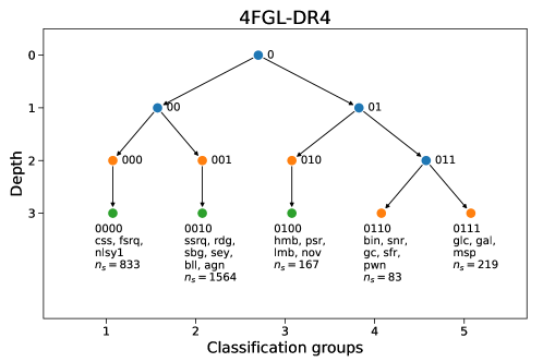
Figure 1: Hierarchical definition of classes following the procedure in refs. [41, 42]. The classes used for the classification in this work are shown at the bottom row (depth 3). The numbers at the bottom show the total count of associated sources in the group.

	Class label	Physical classes	N assoc	RF assoc	NN assoc	RF unas+	NN unas+
1	fsrq+	nlsy1, css, fsrq	833	$838.6\pm 3.0$	$836.0\pm 1.9$	$1153.2\pm 4.5$	$1158.3\pm 3.4$
2	bll+	ssrq, rdg, sbg, sey, bll, agn	1564	$1565.8\pm 3.0$	$1559.6\pm 2.1$	$1796.7\pm 4.4$	$1754.9\pm 2.9$
3	psr+	hmb, psr, lmb, nov	167	$161.5\pm 1.7$	$165.4\pm 2.0$	$408.2\pm 3.5$	$512.0\pm 3.8$
4	snr+	bin, snr, gc, sfr, pwn	83	$80.0\pm 1.3$	$83.1\pm 1.8$	$250.2\pm 2.5$	$231.2\pm 3.4$
5	msp+	glc, gal, msp	219	$220.1\pm 1.9$	$221.9\pm 1.9$	$716.7\pm 4.1$	$668.5\pm 3.4$

Table 2: Definition of classes and prediction for the expected number of class members among associated and unassociated sources. The “unas+” columns include both unassociated sources and sources with uncertain classification (bcu, spp, and unk classes). The table includes predictions based on RF and NN classification algorithms.

Class label	RF unas	NN unas	RF unk	NN unk	RF bcu	NN bcu	RF spp	NN spp
fsrq+	$572.3\pm 3.5$	$563.2\pm 2.8$	$16.6\pm 0.6$	$15.1\pm 0.5$	$550.5\pm 2.8$	$566.3\pm 1.8$	$13.7\pm 0.6$	$13.8\pm 0.6$
bll+	$839.1\pm 3.3$	$808.2\pm 2.3$	$47.4\pm 0.7$	$50.2\pm 0.6$	$891.2\pm 2.8$	$875.7\pm 1.6$	$18.9\pm 0.6$	$20.7\pm 0.6$
psr+	$296.3\pm 3.0$	$375.9\pm 3.3$	$31.1\pm 0.9$	$38.7\pm 0.9$	$45.1\pm 1.2$	$55.4\pm 1.2$	$35.7\pm 1.0$	$42.0\pm 1.0$
snr+	$171.7\pm 2.1$	$157.1\pm 2.9$	$20.3\pm 0.7$	$19.7\pm 1.0$	$32.0\pm 0.9$	$29.5\pm 1.1$	$26.3\pm 0.8$	$24.9\pm 1.0$
msp+	$550.5\pm 3.5$	$525.6\pm 2.9$	$31.5\pm 0.9$	$23.2\pm 0.8$	$105.2\pm 1.6$	$97.1\pm 1.2$	$29.4\pm 0.9$	$22.6\pm 0.8$

Table 3: Predictions for the expected number of class members calculated separately for unassociated, unk, bcu, and spp sources.

In this paper we use two classification algorithms:

1. Random forest (RF) implemented in scikit-learn [44] (version 1.2.2). The maximal number of trees is 50 with the maximal depth 15. For the other parameters we use the default values in the scikit-learn implementation of RF. The RF method is used as a baseline model in the main part of the paper.

2. Neural networks (NN) implemented in TensorFlow [45]. We use stochastic gradient descent (adam) with learning rate of 0.001, two hidden layers with 20 and 10 nodes respectively, tanh activation functions, 2000 epochs, batch size of 200, L2 regularization with $l2=0.001$, and no drop out. We use the sparse categorical cross entropy loss function. Comparison of NN and RF predictions are shown in Appendix A.

We use 70/30% splits into training and testing data samples and derive the class probabilities for all sources (both associated and unassociated). The class probabilities of associated sources are determined by averaging over training/testing splits, when the sources are in testing samples. We require that each associated source appears in the testing samples at least 5 times, which results in 47 training/testing splits. The class probabilities for the unassociated sources (as well as for the unk, bcu, and spp sources, which are not included in the training) are determined by the average over the 47 realizations of the training/testing splits. In the probabilistic catalog we report the class probabilities determined with RF and NN algorithms as well as the corresponding statistical uncertainties derived as a sample average over 47 realizations of training/testing splits for unassociated sources or, for associated sources, as an average over the splits when the source is included in the testing sample.

The number of unassociated sources in class $m$ can be estimated by summing the corresponding class probabilities

$$N_{m}=\sum_{i\in{\rm unas}}p_{m}^{i}.$$ (2.1)

Similarly, one can estimate the number of associated sources in class $m$ (and compare with the actual counts of associated sources in this class) or the number of class-$m$ sources among unk, bcu, or spp sources. In table 2 we show the expected numbers of class members. In this table we add the predictions for the unas, unk, bcu, and spp sources together. The predictions for the unas, unk, bcu, and spp sources separately are presented in table 3. The statistical uncertainty on $N_{m}$ is determined by propagating the uncertainties on the probabilities $p_{m}^{i}$ obtained as a standard deviation of predicted probabilities for the different training/testing splits: $\sigma(N_{m})=\sqrt{\sum_{i\in{\rm unas}}\sigma(p_{m}^{i})^{2}}$. The expected number of sources in a class among associated sources is computed analogously to the unassociated sources, where the sum in eq. 2.1 goes over all associated rather than unassociated sources. As one can see in table 2, the predicted numbers of class members among associated sources are consistent with the actual source counts of associated sources. RF and NN algorithms agree on the predicted numbers of bll+, fsrq+, and snr+ sources among the unassociated sources, but have rather different predictions for psr+ and msp+ classes. This is not surprising, provided that the gamma-ray spectra of MSPs and young pulsars are similar, while the spatial distribution of these sources is not taken into account for training. If we add the predicted numbers of sources in psr+ and msp+ classes (1125 and 1181 for RF and NN algorithms respectively), then the difference of about 56 sources is comparable to (smaller than) the difference of 48 sources (104 sources) in prediction for the msp+ (psr+) class alone.

3 Distribution of unassociated MSP-like sources

3.1 Energy spectrum

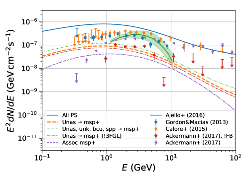
Figure 2: Comparison of the GCE SED with the SED from MSP-like sources within $10^{\circ}$ from the GC. Blue solid line – combined SED for all 4FGL-DR4 sources within $10^{\circ}$ from the GC, orange dashed line – the expected contribution from msp+ sources among the unassociated sources, green dotted line – the expected contribution from msp+ sources among the unassociated, unk, bcu, spp sources, red dash-dotted line – the expected contribution from msp+ sources among the unassociated sources after excluding the sources detected in the 3FGL catalog, purple dash-dot-dotted line – SED for the associated MSPs. The GCE models include Gordon&Macias (2013) [6], Calore+ (2015) [8], Ajello+ (2016) [10]. The label “Ackermann+ (2017), !FB” (“Ackermann+ (2017)”) corresponds to a model in ref. [11] that that takes (does not take) into account the contribution from Fermi bubbles near the GC.

In this section we derive the expected combined SED that can be attributed to the msp+ class near the GC. We consider sources within $10^{\circ}$ from the GC and determine the SED by summing the log-parabola spectra weighted by the msp+ class probabilities. For example, the expected contribution of the msp+ class to the SED of unassociated sources is determined as

$$F_{\rm msp+}(E)=\sum_{i\in{\rm unas}}p_{\rm msp+}^{i}F_{i}(E),$$ (3.1)

where $p_{\rm msp+}^{i}$ is the msp+ class probability for source $i$ and $F_{i}(E)$ is the SED for source $i$ modeled by the log-parabola spectrum. The corresponding msp+ SED is shown in figure 2 by the orange dashed line (labeled as “Unas $\rightarrow$ msp+”). If we sum over all unas, unk, bcu, and spp sources in eq. (3.2), then the expected SED is shown by the green dotted line (labeled as “Unas, unk, bcu, spp $\rightarrow$ msp+”). We see that the effect of including unk, bcu, spp sources in addition to the unassociated ones is relatively small. The contribution of the 4FGL-DR4 unassociated sources, which do not have a counterpart in the 3FGL catalog is shown by the red dash-dotted line (labeled as “Unas $\rightarrow$ msp+ (!3FGL)”). This is the emission, which was previously not resolved in the 3FGL catalog and must have been attributed to a diffuse-like component, e.g., the GCE. For comparison, the combined SED of all resolved (all associated msp+) sources in the ROI is shown by the blue solid (purple dash-dot-dotted) line. We compare the msp+ SED with the GCE SEDs from refs. [6, 8, 10, 11]. We note that different analyses of GCE have slightly different ROIs. Provided that we are interested in a qualitative agreement, we take the ROIs which are closest to the circle of $10^{\circ}$ radius around the GC and apply no correction for the differences in the ROI. For the analysis of Ajello et al (2016) [10] (green band), we use the model with CR sources traced by pulsars and both the normalization and the index of the background components are fitted. For the analysis of Ackerman et al (2017) [11], we include the baseline model that does not have a model of the Fermi bubbles below $10^{\circ}$ in latitude (blue squares) and a model where a possible emission of the Fermi bubbles near the GC in figure 9 of ref. [11] is taken into account (red diamonds with “!FB” in the label). It is particularly interesting, that the contribution of the msp+ class to the unassociated sources (also when sources with the 3FGL counterparts are not included) is comparable to the SED attributed to the GCE in a model that removes a possible emission from the Fermi bubbles at low latitudes. Thus, it is possible that the GCE, after taking into account emission from the Fermi bubbles, is resolved into sources with MSP-like properties in the 4FGL-DR4 catalog.

3.2 Radial profile

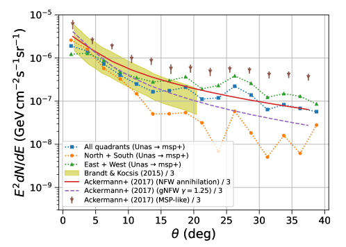
Figure 3: Radial profile of expected intensity from msp+ sources at 2 GeV defined in eq. (3.2). Blue squares, orange circles, and green triangles show respectively the intensity in all, North+South, East+West quadrants. For comparison, we show the GCE profiles (divided by 3 to account for possible effect of the subtraction of the Fermi bubbles) from Brandt & Kocsis (2015) [14] and Ackermann et al (2017) [11]. See text for more details.

We compare in figure 3 the radial profile of the unassociated msp+ component to the radial profiles of GCE models at 2 GeV. The average intensity of the msp+ component of the unassociated sources in a ring between $\theta_{1}$ and $\theta_{2}$ from the GC is estimated as

$$I_{\rm msp+}(\theta)=\frac{1}{\Omega}\sum_{i\in{\rm unas},\ \theta_{i}\in(\theta_{1},\ \theta_{2})}p_{\rm msp+}^{i}F_{i}(E=2\ {\rm GeV}),$$ (3.2)

where $\theta=(\theta_{1}+\theta_{2})/2$ is the mean radius and $\Omega$ is the solid angle of the ring. The radial profile of the expected intensity of emission at 2 GeV for the msp+ component among the unassociated sources is shown by the blue squares in figure 3. We also separately plot the intensities in the North+South quadrants (orange circles) and East+West quadrants (green upward triangles). Assuming that the inclusion of the Fermi bubbles near the GC in the model potentially reduces the flux attributed to the GCE by about a factor of 3 at 2 GeV (cf. figure 2), we divide the models listed below by 3. The model for the MSP population derived from disrupted globular clusters [14] is shown by the yellow band. We also consider several models from ref. [11]: the NFW DM annihilation profile (solid red line), the generalized NFW DM annihilation profile with index $\gamma=1.25$ (dashed purple line), and a model of the GCE derived from a correlation with MSP-like energy spectrum (figure 11 of ref. [11]) shown by the brown downward triangles.

The average profile and the North+South, East+West profiles have a reasonable agreement with the NFW (or gNFW) DM annihilation profiles within about $10^{\circ}$ from the GC. At larger separations, the East+West (North+South) distribution is flatter (steeper) than the NFW profile. We interpret this difference as a contribution of two different populations of MSPs: the bulge population that has an approximately spherical distribution around the GC, which dominates the intensity within $10^{\circ}$ from the GC and a disk component, which dominates the emission for the East+West quadrants further away from the GC and is largely absent in the North+South quadrants.

It is interesting to note that the intensity of excess emission derived from the correlation with the MSP-like energy spectrum (the brown downward triangles in figure 3) is generally higher than the other GCE profiles (cf. ref. [11]), it is also higher than the distribution of the msp+ component among the unassociated sources (even after dividing by the factor of 3). This may be due to a further contribution from an unresolved population of MSPs. In addition, there is potentially an important contribution from young pulsars (Appendix B).

3.3 Source count distribution

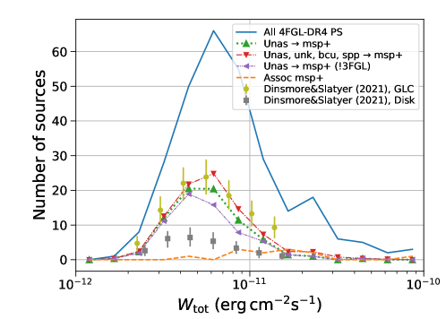
Figure 4: Distribution of the expected source count for the msp+ component of unassociated sources as a function of energy flux integrated above 100 MeV. Blue solid line – all sources in the 4FGL-DR4 catalog detected within $10^{\circ}$ from the GC, green upward (red downward) triangles – expected msp+ contribution among unassociated (unassociated, unk, bcu, and spp) sources, purple left triangles – msp+ contribution to unassociated sources after excluding sources detected in the 3FGL catalog. Orange dashed line – distribution of associated msp+ sources. We compare the distributions with two models of MSPs with luminosity functions scaled to reproduce the GCE (figure 9a of ref. [20]): a model based on the properties of globular clusters [38] – yellow circles labeled as “GLC”, and a model based on the properties of MSPs in the Galactic disk [18] – grey squares labeled as “Disk”.

The number of msp+ sources among the unassociated sources with integrated energy fluxes $W_{i}\in(W_{1},\ W_{2})$ is estimated as

$$N_{\rm msp+}(W)=\sum_{i\in{\rm unas},\ W_{i}\in(W_{1},\ W_{2})}p_{\rm msp+}^{i},$$ (3.3)

where $W_{i}$ is the energy flux above 100 MeV for an unassociated source $i$ (we use the “Energy_Flux100” values in the catalog) and $W$ is the logarithmic center of the bin: $W=\sqrt{W_{1}W_{2}}$. In figure 4 we show the source count distribution (for sources within $10^{\circ}$ from the GC) for the msp+ component of unassociated sources (green upward triangles), of unassociated, unk, bcu, and spp sources (red downward triangles), of unassociated sources, where the 3FGL sources are excluded (purple left triangles). We also show the distributions (within the $10^{\circ}$ radius from the GC) for all 4FGL-DR4 sources (solid blue line) and for associated msp+ sources (dashed orange line). We compare the distributions with two models of MSPs with luminosity functions scaled to reproduce the GCE (figure 9a of ref. [20]): a model based on the properties of globular clusters [38] – yellow circles labeled as “GLC”, and a model based on the properties of MSPs in the Galactic disk [18] – grey squares labeled as “Disk”. These two models provide reasonable benchmark cases for many other models of the MSP luminosity functions, e.g., refs. [23, 24, 17, 46, 47, 48]. Interestingly, the expected number of msp+ sources among the unassociated sources in the 4FGL-DR4 catalog seem to favor the luminosity function for MSPs derived from the globular clusters [38].

We note that the luminosity function of the GLC model [38] is normalized in ref. [20] to reproduce the full GCE. Although the flux from the MSP-like candidates is about a factor three smaller than the full GCE SED, the expected source count of MSP-like sources in figure 4 is consistent with the expected number of MSPs that can be detected by the Fermi LAT. The reason for this apparent discrepancy is that, although the luminosity function of the GLC model is dominated by bright sources relative to most of other models of the MSP population near the GC, the peak of the luminosity function in the GLC model is still below the Fermi-LAT flux sensitivity. In particular, the Fermi-LAT sensitivity is estimated to be about $4\times 10^{-12}\ {\rm erg\,cm^{-2}s^{-1}}$ (Figure 5 of ref. [20]), while the peak in $LdN/dL$ distribution is at about $4\times 10^{-13}\ {\rm erg\,cm^{-2}s^{-1}}$ (Figure 7 of ref. [20]). Thus also in the GLC model the majority of the GCE SED is expected to come from MSPs undetected by the Fermi LAT.

4 Conclusions and discussion

In this paper we performed a multi-class classification of Fermi-LAT sources into five classes dominated by fsrq, bll, psr, snr, and msp classes. We excluded unk, bcu, and spp classes from training of machine learning classification algorithms since the nature of the association counterparts is either unknown or uncertain for these classes. One of the biggest effects from excluding unk, bcu, and spp classes from training is that these classes are also excluded from the classification of the unassociated sources. As a result, the expected number of, e.g., MSP-like sources among the unassociated ones is much larger in this case, compared to a classification where bcu and spp sources are included in training and classification [41, 42].

We find that a significant fraction of GCE is now resolved into point sources consistent with MSP-like sources. If we take into account a possible contribution from the Fermi bubbles, then the contribution of the MSP-like sources becomes comparable to the remaining GCE flux around a few GeV. Although this results shows the potential that the problem of the GCE can be resolved by detecting individual gamma-ray sources near the GC. There are, however, several caveats in the analysis, which require a further investigation:

1. The spectrum of the msp+ component is relatively flat below 1 GeV while the spectrum of GCE determined in some analyses, including the analysis that takes the FB into account [11], is hard below 1 GeV. The GCE spectrum at low energies has large systematic uncertainties, i.e., it can also be relatively soft [6]. This question can be resolved by an updated analysis of the gamma-ray data near the GC that includes the 4FGL-DR4 sources.

2. The uncertainties in the diffuse emission model affect also the detectability and the properties of point-like sources. In particular, many sources near the GC in the 4FGL-DR4 catalog have flags, which denote different problems either with detection of the sources or with reconstruction of their properties (the corresponding effect on the SED can be significant, as discussed in Appendix A).

3. The separation of the GCE from the Fermi bubbles is one of the biggest uncertainties that can have a factor two to three effect on the GCE spectrum around a few GeV [11].

Although the study presented in this work shows that the GCE can be resolved into individual point-like sources consistent with MSP properties, in view of the above caveats, a detailed joint analysis of the diffuse emission and point-like sources as well as a study of the Fermi bubbles near the GC will be necessary to resolve the GCE puzzle. A significant progress can be also made by multi-wavelength searches for counterparts of gamma-ray sources, e.g., radio emission from MSPs.

Appendix A Systematic uncertainties

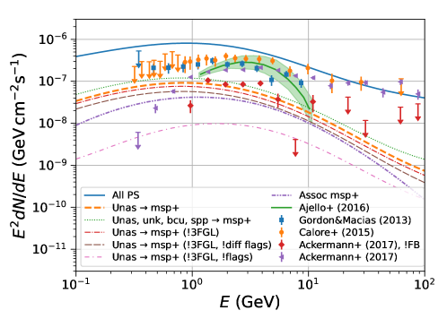
Figure 5: Effect of removing sources with analysis flags on the expected msp+ SED. Brown long-dashed line shows the effect of removing the sources, which become insignificant as a result of changes in the diffuse emission models, which are correlated with dense gas clumps, or which have TS $<25$ (flags 1, 6, or 13 respectively in the 4FGL-DR4 catalog [40]). Pink sparse dash-dotted line shows the effect of removing all flagged sources in the 4FGL-DR4 catalog. See figure 2 for the definition of the other lines and points.

In this appendix we check the dependence of the predictions for the msp+ component among unassociated sources on the choice of the classification algorithm, uncertainties in the background diffuse emission, classification with or without bcu and spp sources, and the use of weighting to account for differences in the distributions of associated and unassociated sources. In figure 5 we show the SED for the msp+ component of unassociated sources by the orange dashed line. The msp+ component of unassociated sources together with bcu, spp, and unk sources is shown by the green dotted line. The msp+ component of unassociated sources excluding the sources, which were already detected in the 3FGL catalog is shown by the red dash-dotted line (the change is relatively small, which means that the majority of the msp+ contribution in the 4FGL catalog is newly resolved compared to the 3FGL catalog). Some sources in the catalog may be false detections due to uncertainties in the gamma-ray diffuse background model. The brown long-dashed line shows the msp+ component of unassociated sources after removing the sources with the following flags [40] (referred to as diffuse flags below): (1) TS $<$ 25 with other model or analysis, (6) Interstellar gas clump (c sources), (13) TS $<$ 25. Here we also remove sources detected in the 3FGL catalog (the label has “!3FGL, !diff flags”). The effect of these three flags is relatively little. Removing all flagged sources reduces the msp+ SED by almost a factor 10 (pink sparse dash-dotted line), which shows that there are potentially problems with detection and reconstruction of spectra and / or positions of sources near the GC. Thus, many of the sources near the GC in the 4FGL-DR4 catalog may be spurious or have uncertain characteristics. For comparison we also show the combined SED of all resolved (all associated msp+) sources in the ROI by the blue solid (purple dash-dot-dotted) line.

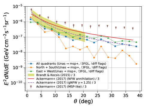
Figure 6: Effect of removing sources detected in the 3FGL catalog and sources with diffuse analysis flags (flags 1, 6, or 13 respectively in the 4FGL-DR4 catalog [40]) on the expected radial distribution of the msp+ component. Lines and points are the same as in figure 3 but we exclude unassociated sources detected in the 3FGL catalog and the sources with diffuse analysis flags.

The average radial profile and the profiles in North+South or East+West quadrants of the MSP-like component after removing sources detected in the 3FGL catalog and sources with the diffuse analysis flags are shown in figure 6. The profiles are similar to the profiles in figure 3 with the overall normalization reduced by about 40%.

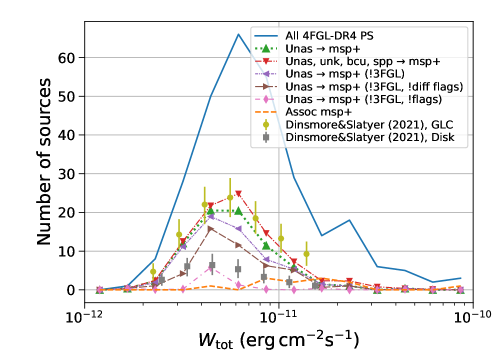
Figure 7: Effect of removing sources with diffuse analysis flags (brown right triangles) and all analysis flags (pink diamonds) on the source count distribution of the msp+ component. The other lines and points are the same as in figure 4.

The effect of removing sources with analysis flags on the source count distribution is shown in figure 7. Diffuse analysis flags (flags 1, 6, or 13 in the 4FGL-DR4 catalog [40]) have relatively little effect on the source count distribution and they mostly affect sources with energy flux below about $10^{-11}\ {\rm erg\,cm^{-2}s^{-1}}$. Although the source count distribution after removing sources with diffuse analysis flags seems to be inconsistent with the GLC model, one should take into account the effect of removing the flagged sources on the source sensitivity model used in ref. [20] to determine the predicted source count distributions of sources detected by the Fermi LAT that can explain the GC excess. Removing all sources with flags has a rather large effect on the source count distribution. However, one should also take into account the effect on the Fermi-LAT source detection sensitivity. In addition, some flags are given to sources, which are unstable with respect to a change in the diffuse emission model (e.g., a source moves outside of the 95% containment ellipse), but the sources themselves do not disappear. As a result, removing sources with all analysis flags is likely a too conservative approach to estimate the contribution of point-like sources in the ROI.

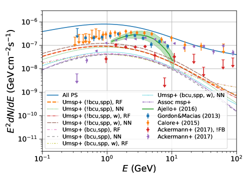
Figure 8: Effect of the choice of the classification algorithm (RF or NN), of excluding or including bcu and spp sources in training (!bcu, spp or bcu, spp in labels), and of using unweighted or weighted loss to account for differences in the distribution of associated and unassociated sources (weighted loss is shown by “w” in labels) on the msp+ contribution to the SED of unassociated sources. “Umsp+” shows the contribution of the msp+ class to the unassociated sources. See figure 2 for the definition of the other lines and points.

In figure 8 we show the effect of several choices in classification algorithms on the SED of the msp+ component of the unassociated sources (denoted as “Umsp+” in the labels). The classification with RF and NN algorithms is denoted by “RF” and “NN” in the labels respectively. In order to account for the differences in the distributions of associated and unassociated sources, we introduce the weights proportional to the ratio of probability distribution functions of unassociated to associated sources [42]. Training with associated sources weighted by the corresponding weights is shown by “w” in the labels. The choice of the classification algorithms and the use of weighting have relatively little effect on the predicted SED of the msp+ component of the unassociated sources. The last effect that we test is the inclusion of bcu and spp classes in training. The definition of the groups, when bcu and spp classes are included in training, as well as predictions for the overall number of unassociated and unk sources attributed to the six class are shown in table 4. The corresponding SEDs for the msp+ component of unassociated sources when the bcu and spp classes are included in training (“bcu,spp” in labels) are a factor of 2 to 3 smaller than the SEDs for training without bcu and spp classes (“!bcu,spp” in labels).

	Class	Physical classes	N assoc	RF assoc	NN assoc	RF unas,unk	NN unas,unk
1	psr+	hmb, snr, gc, pwn, psr	219	$211.8\pm 1.9$	$214.3\pm 2.1$	$158.7\pm 2.0$	$164.8\pm 1.5$
2	msp+	lmb, msp, gal, glc, bin, sfr	244	$245.9\pm 2.1$	$247.4\pm 1.9$	$273.3\pm 2.4$	$271.0\pm 1.5$
3	spp+	spp, nov	130	$127.5\pm 1.8$	$127.9\pm 1.6$	$367.5\pm 3.0$	$398.5\pm 2.8$
4	fsrq+	nlsy1, fsrq	827	$832.5\pm 3.7$	$827.1\pm 2.3$	$205.4\pm 2.2$	$187.0\pm 1.2$
5	bll+	ssrq, css, bll, sey	1501	$1504.5\pm 4.3$	$1515.8\pm 2.4$	$328.9\pm 2.5$	$305.8\pm 1.3$
6	bcu+	agn, sbg, bcu, rdg	1693	$1691.8\pm 5.1$	$1681.5\pm 2.9$	$1243.3\pm 4.2$	$1249.9\pm 2.9$

Table 4: Definition of classes and prediction for unassociated sources together with the unk physical class in case bcu and spp sources are included in training [42].

Appendix B Contribution of young pulsars to GCE

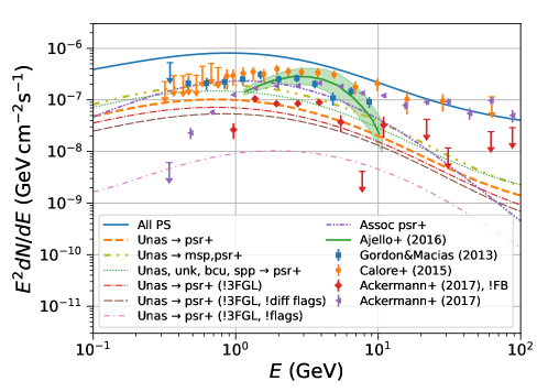
Figure 9: Contribution of the psr+ class to the SED of unassociated sources within $10^{\circ}$ from the GC. Yellow sparse dash-dot-dotted line shows the combined contribution of msp+ and psr+ sources. The other lines are either the same as in figures 2 and 5 or the msp+ contribution is replaced by the psr+ contribution.

A population of young pulsars has been proposed as one of the possible explanations of the GCE [21]. In this appendix we consider the contribution of the psr+ component among the unassociated sources to the gamma-ray flux near the GC. Figure 9 shows the SED for the psr+ component of unassociated sources within $10^{\circ}$ from the GC (orange dashed line). The contribution from the psr+ class is comparable to the msp+ component (orange dashed line in Figures 2, 5, and 8). We also show the combined contribution from psr+ and msp+ classes (shown by the yellow sparse dash-dot-dotted line in figure 9). The combined psr+ and msp+ SED is now above the possible GCE SED if the Fermi bubbles are taken into account and just below the GCE, where the Fermi bubbles are not modeled or modeled with the same intensity as at high latitudes. As in figure 5, we also check the effect of excluding the 3FGL sources as well as excluding sources with flags. Similarly to the msp+ case, excluding 3FGL sources and diffuse flags (1, 6, and 13) has relatively little effect on the SED, while excluding all flagged sources reduces the SED by a factor 10. Interestingly, the combined SED of associated psr+ sources in this ROI (purple dash-dot-dotted line in figure 9) is about a factor two larger than the SED of the psr+ component of unassociated sources, while the SED of associated msp+ sources (purple dash-dot-dotted line in figure 5) is about a factor two smaller than the msp+ component of unassociated sources.

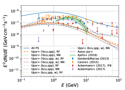
Figure 10: Effect of the choice of the classification algorithm, of excluding or including bcu and spp sources in training, and of using unweighted or weighted loss on the psr+ contribution to the SED of unassociated sources. For the definition of lines see figures 2 and 8 where the msp+ contribution is replaced by the psr+ contribution (when relevant).

In figure 10 we test the effect of the choice of classification algorithm (RF vs NN), weighted or unweighted training, and including or not including bcu and spp classes in training. In this case, even excluding bcu and spp sources from training has relatively little effect on the expected psr+ SED.

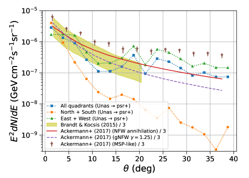
Figure 11: Contribution of the psr+ class to the radial intensity profile of unassociated sources at 2 GeV. The lines are defined as in figure 3 with the msp+ contribution replaced by the psr+ contribution (when relevant).

The radial profile of the psr+ component is shown in figure 11. In this case the averaged profile is similar to the NFW DM annihilation profile. However, in the East+West (North+South) quadrants the psr+ profile is flatter (steeper) than the NFW annihilation profile. This is expected for the distribution of young pulsars, since they cannot travel far from the locations where they are created due to relatively short lifetime. As a result, the young pulsars are distributed close to the Galactic plane. Thus, although, the SED of the psr+ component is comparable to the msp+ component and to the expected GCE SED (after excluding a possible contribution from the Fermi bubbles), the psr+ sources have a distribution along the Galactic plane, which is different from the more spherical distribution of the gamma-ray excess around the GC as well as the distribution of the msp+ component.

References

- [1] L. Goodenough and D. Hooper, Possible Evidence For Dark Matter Annihilation In The Inner Milky Way From The Fermi Gamma Ray Space Telescope, arXiv e-prints (2009) arXiv:0910.2998 [0910.2998].
- [2] V. Vitale and A. Morselli, Indirect Search for Dark Matter from the center of the Milky Way with the Fermi-Large Area Telescope, arXiv e-prints (2009) arXiv:0912.3828 [0912.3828].
- [3] D. Hooper and L. Goodenough, Dark matter annihilation in the Galactic Center as seen by the Fermi Gamma Ray Space Telescope, Physics Letters B 697 (2011) 412 [1010.2752].
- [4] D. Hooper and T. Linden, Origin of the gamma rays from the Galactic Center, PRD 84 (2011) 123005 [1110.0006].
- [5] K.N. Abazajian and M. Kaplinghat, Detection of a gamma-ray source in the Galactic Center consistent with extended emission from dark matter annihilation and concentrated astrophysical emission, PRD 86 (2012) 083511 [1207.6047].
- [6] C. Gordon and O. Macías, Dark matter and pulsar model constraints from Galactic Center Fermi-LAT gamma-ray observations, PRD 88 (2013) 083521 [1306.5725].
- [7] D. Hooper and T.R. Slatyer, Two emission mechanisms in the Fermi Bubbles: A possible signal of annihilating dark matter, Physics of the Dark Universe 2 (2013) 118 [1302.6589].
- [8] F. Calore, I. Cholis and C. Weniger, Background model systematics for the Fermi GeV excess, JCAP 2015 (2015) 038 [1409.0042].
- [9] T. Daylan, D.P. Finkbeiner, D. Hooper, T. Linden, S.K.N. Portillo, N.L. Rodd et al., The characterization of the gamma-ray signal from the central Milky Way: A case for annihilating dark matter, Physics of the Dark Universe 12 (2016) 1 [1402.6703].
- [10] M. Ajello, A. Albert, W.B. Atwood et al., Fermi-LAT Observations of High-Energy Gamma-Ray Emission toward the Galactic Center, ApJ 819 (2016) 44.
- [11] M. Ackermann, M. Ajello, A. Albert et al., The Fermi Galactic Center GeV Excess and Implications for Dark Matter, ApJ 840 (2017) 43 [1704.03910].
- [12] K.N. Abazajian, The consistency of Fermi-LAT observations of the galactic center with a millisecond pulsar population in the central stellar cluster, JCAP 2011 (2011) 010 [1011.4275].
- [13] J. Petrović, P.D. Serpico and G. Zaharijas, Millisecond pulsars and the Galactic Center gamma-ray excess: the importance of luminosity function and secondary emission, JCAP 2015 (2015) 023 [1411.2980].
- [14] T.D. Brandt and B. Kocsis, Disrupted Globular Clusters Can Explain the Galactic Center Gamma-Ray Excess, ApJ 812 (2015) 15 [1507.05616].
- [15] O. Macias, C. Gordon, R.M. Crocker, B. Coleman, D. Paterson, S. Horiuchi et al., Galactic bulge preferred over dark matter for the Galactic centre gamma-ray excess, Nature Astronomy 2 (2018) 387 [1611.06644].
- [16] R. Bartels, E. Storm, C. Weniger and F. Calore, The Fermi-LAT GeV excess as a tracer of stellar mass in the Galactic bulge, Nature Astronomy 2 (2018) 819 [1711.04778].
- [17] P.L. Gonthier, A.K. Harding, E.C. Ferrara, S.E. Frederick, V.E. Mohr and Y.-M. Koh, Population Syntheses of Millisecond Pulsars from the Galactic Disk and Bulge, ApJ 863 (2018) 199 [1806.11215].
- [18] R.T. Bartels, T.D.P. Edwards and C. Weniger, Bayesian model comparison and analysis of the Galactic disc population of gamma-ray millisecond pulsars, MNRAS 481 (2018) 3966 [1805.11097].
- [19] O. Macias, S. Horiuchi, M. Kaplinghat, C. Gordon, R.M. Crocker and D.M. Nataf, Strong evidence that the galactic bulge is shining in gamma rays, JCAP 2019 (2019) 042 [1901.03822].
- [20] J.T. Dinsmore and T.R. Slatyer, Luminosity functions consistent with a pulsar-dominated Galactic Center excess, JCAP 2022 (2022) 025 [2112.09699].
- [21] R.M. O’Leary, M.D. Kistler, M. Kerr and J. Dexter, Young Pulsars and the Galactic Center GeV Gamma-ray Excess, arXiv e-prints (2015) arXiv:1504.02477 [1504.02477].
- [22] S.K. Lee, M. Lisanti and B.R. Safdi, Distinguishing dark matter from unresolved point sources in the Inner Galaxy with photon statistics, JCAP 2015 (2015) 056 [1412.6099].
- [23] R. Bartels, S. Krishnamurthy and C. Weniger, Strong Support for the Millisecond Pulsar Origin of the Galactic Center GeV Excess, PRL 116 (2016) 051102 [1506.05104].
- [24] S.K. Lee, M. Lisanti, B.R. Safdi, T.R. Slatyer and W. Xue, Evidence for Unresolved -Ray Point Sources in the Inner Galaxy, PRL 116 (2016) 051103 [1506.05124].
- [25] R.K. Leane and T.R. Slatyer, Revival of the Dark Matter Hypothesis for the Galactic Center Gamma-Ray Excess, PRL 123 (2019) 241101.
- [26] R.K. Leane and T.R. Slatyer, Spurious Point Source Signals in the Galactic Center Excess, PRL 125 (2020) 121105 [2002.12370].
- [27] R.K. Leane and T.R. Slatyer, The enigmatic Galactic Center excess: Spurious point sources and signal mismodeling, PRD 102 (2020) 063019 [2002.12371].
- [28] L.J. Chang, S. Mishra-Sharma, M. Lisanti, M. Buschmann, N.L. Rodd and B.R. Safdi, Characterizing the nature of the unresolved point sources in the Galactic Center: An assessment of systematic uncertainties, PRD 101 (2020) 023014 [1908.10874].
- [29] M. Buschmann, N.L. Rodd, B.R. Safdi, L.J. Chang, S. Mishra-Sharma, M. Lisanti et al., Foreground mismodeling and the point source explanation of the Fermi Galactic Center excess, PRD 102 (2020) 023023 [2002.12373].
- [30] F. List, N.L. Rodd, G.F. Lewis and I. Bhat, Galactic Center Excess in a New Light: Disentangling the -Ray Sky with Bayesian Graph Convolutional Neural Networks, PRL 125 (2020) 241102 [2006.12504].
- [31] F. List, N.L. Rodd and G.F. Lewis, Extracting the Galactic Center excess’ source-count distribution with neural nets, PRD 104 (2021) 123022 [2107.09070].
- [32] J. Petrović, P.D. Serpico and G. Zaharijaš, Galactic Center gamma-ray “excess” from an active past of the Galactic Centre?, JCAP 2014 (2014) 052 [1405.7928].
- [33] I. Cholis, C. Evoli, F. Calore, T. Linden, C. Weniger and D. Hooper, The Galactic Center GeV excess from a series of leptonic cosmic-ray outbursts, JCAP 2015 (2015) 005 [1506.05119].
- [34] E. Carlson, S. Profumo and T. Linden, Cosmic-Ray Injection from Star-Forming Regions, PRL 117 (2016) 111101 [1510.04698].
- [35] M. Pohl, O. Macias, P. Coleman and C. Gordon, Assessing the Impact of Hydrogen Absorption on the Characteristics of the Galactic Center Excess, ApJ 929 (2022) 136 [2203.11626].
- [36] I. Cholis, Y.-M. Zhong, S.D. McDermott and J.P. Surdutovich, Return of the templates: Revisiting the Galactic Center excess with multimessenger observations, PRD 105 (2022) 103023 [2112.09706].
- [37] F. Calore, M. Di Mauro, F. Donato, J.W.T. Hessels and C. Weniger, Radio Detection Prospects for a Bulge Population of Millisecond Pulsars as Suggested by Fermi-LAT Observations of the Inner Galaxy, ApJ 827 (2016) 143 [1512.06825].
- [38] D. Hooper and T. Linden, The gamma-ray pulsar population of globular clusters: implications for the GeV excess, JCAP 2016 (2016) 018 [1606.09250].
- [39] D. Haggard, C. Heinke, D. Hooper and T. Linden, Low mass X-ray binaries in the Inner Galaxy: implications for millisecond pulsars and the GeV excess, JCAP 2017 (2017) 056 [1701.02726].
- [40] J. Ballet, P. Bruel, T.H. Burnett, B. Lott and The Fermi-LAT collaboration, Fermi Large Area Telescope Fourth Source Catalog Data Release 4 (4FGL-DR4), arXiv e-prints (2023) arXiv:2307.12546 [2307.12546].
- [41] D.V. Malyshev and A. Bhat, Multiclass classification of Fermi-LAT sources with hierarchical class definition, MNRAS 521 (2023) 6195 [2301.07412].
- [42] D.V. Malyshev, Effect of covariate shift on multi-class classification of Fermi-LAT sources, RAS Techniques and Instruments 2 (2023) 735 [2307.09584].
- [43] S. Abdollahi, F. Acero, L. Baldini, J. Ballet, D. Bastieri, R. Bellazzini et al., Incremental Fermi Large Area Telescope Fourth Source Catalog, ApJS 260 (2022) 53 [2201.11184].
- [44] F. Pedregosa, G. Varoquaux, A. Gramfort, V. Michel, B. Thirion, O. Grisel et al., Scikit-learn: Machine learning in Python, Journal of Machine Learning Research 12 (2011) 2825.
- [45] M. Abadi, A. Agarwal, P. Barham, E. Brevdo, Z. Chen, C. Citro et al., TensorFlow: Large-scale machine learning on heterogeneous systems, 2015.
- [46] Y.-M. Zhong, S.D. McDermott, I. Cholis and P.J. Fox, Testing the Sensitivity of the Galactic Center Excess to the Point Source Mask, PRL 124 (2020) 231103 [1911.12369].
- [47] H. Ploeg, C. Gordon, R. Crocker and O. Macias, Comparing the galactic bulge and galactic disk millisecond pulsars, JCAP 2020 (2020) 035 [2008.10821].
- [48] A. Gautam, R.M. Crocker, L. Ferrario, A.J. Ruiter, H. Ploeg, C. Gordon et al., Millisecond pulsars from accretion-induced collapse as the origin of the Galactic Centre gamma-ray excess signal, Nature Astronomy 6 (2022) 703 [2106.00222].
- [49] T.P. Robitaille, E.J. Tollerud, P. Greenfield et al., Astropy: A community Python package for astronomy, A&A 558 (2013) A33 [1307.6212].
- [50] J.D. Hunter, Matplotlib: A 2d graphics environment, Computing In Science & Engineering 9 (2007) 90.
- [51] W. McKinney, Data Structures for Statistical Computing in Python, in Proceedings of the 9th Python in Science Conference, Stéfan van der Walt and Jarrod Millman, eds., pp. 56 – 61, 2010, DOI.