Joint Order Selection, Allocation, Batching and Picking for Large Scale Warehouses

Abstract

Order picking is the single most cost-intensive activity in picker-to-parts warehouses, and as such has garnered large interest from the scientific community which led to multiple problem formulations and a plethora of algorithms published. Unfortunately, most of them are not applicable at the scale of really large warehouses like those operated by Zalando, a leading European online fashion retailer.

Based on our experience in operating Zalando’s batching system, we propose a novel batching problem formulation for mixed-shelves, large scale warehouses with zoning. It brings the selection of orders to be batched into the scope of the problem, making it more realistic while at the same time increasing the optimization potential.

We present two baseline algorithms and compare them on a set of generated instances. Our results show that first, even a basic greedy algorithm requires significant runtime to solve real-world instances and second, including order selection in the studied problem shows large potential for improved solution quality.

1 Introduction

In manual picker-to-parts warehouses, order picking (the process of collecting items from the warehouse floor in order to fulfill customer orders) constitutes more than 55% of the total warehouse cost [25]. On top of that, about 50% of picker’s time is spent traveling between picked items’ locations [16]. Hence, optimizing the process in general, and minimizing its walking component in particular, have been at the heart of many researchers’ interests.

1.1 Context

In this section, we describe aspects of warehouse order picking that are relevant in the setting considered in this paper. The overall problem entails decisions made on a few levels and, consequently, a few optimization problems modeling various parts of it have been introduced and studied. We start with an overview of the most prominent ones. Please refer to the surveys [3] and [2] for a more complete picture.

Picker routing.

At the lowest level, items assigned to a picker need to be collected in a single tour. As other time components (setup time, searching for items and picking them) are usually considered static, travel time is the one aspect which is subject to optimization [9]. As already mentioned, it also accounts for a significant share of the time spent on the picking process, so it is only logical to try to optimize it.

This optimization problem is captured by the Picker Routing Problem (PRP, see [12, 13]): given a set of item locations a picker should visit, the goal is to produce an ordered picklist which is a complete description of a picker’s desired walking route through (a part of) the warehouse. A standard approach to optimization of travel time is to consider minimization of the distance traveled along the picklist [15, 5, 8].

Order batching.

To benefit from economies of scale, items belonging to different customer orders are often picked together [3]. This is the main idea behind batching – grouping customer orders together for joint picking. In the general sense, a batch is defined as a logical grouping of a number of orders, together with a set of related picklists containing exactly the items assigned to the orders forming the batch. The goal of the problem is to create batches covering all orders, with the objective of minimizing the sum of lengths of all involved picklists.

A commonly studied formalization of the problem is known as the Order Batching Problem (OBP), (see, e.g., [20]). In this publication, a batch is equivalent to a picklist, meaning that there is exactly one picklist per batch. In other variants of the problem, multiple picklists per batch are permitted [7, 24].

Integrated solutions.

Given that the objective in the batching problem (OBP) is to minimize total length of picker routes, it comes as no surprise that a joint order batching and picking problem was widely studied, starting with [22]. Sometimes, other planning aspects such as pick scheduling are included in the considered problem as well, e.g., see [18, 14]. This direction of research, summarized in [19] and [2], has produced superior results over approaches treating subproblems of order picking separately.

We continue with a description of how order picking is organized in the large-scale warehouses we study.

Mixed-shelves storage.

As mentioned in [1], a mixed-shelves storage policy is employed in large scale logistics facilities of e-commerce companies the likes of Amazon and Zalando. Warehouses operating under this storage policy do not prescribe a specific storage location where all items of a particular SKU are to be stored. Instead, items of the same SKU can be stored in arbitrary locations throughout the warehouse [6].

Such spread happens organically when an unsupervised storage policy is utilized, i.e. when workers freely decide where to put the items. Going a step further, the explosive storage policy [11] prescribes a concerted effort be taken in order to distribute arriving items of an SKU all over the warehouse.

Employing a mixed-shelves storage policy introduces another decision to be made in the order picking landscape, namely item assignment: deciding which items and, most importantly, from which locations to fulfill an order. Whereas item assignment was considered predetermined and part of the input in many classic approaches, recent research [21, 23] has shown that incorporating it into the considered problem leads to improved order picking efficiency.

Zoning.

Even under the mixed-shelves storage policy, distances between items assigned to the same order can easily become big in large scale warehouses, making it inefficient to collect all items of an order in a single tour.

To deal with this problem and improve pick locality, warehouses are subdivided into distinct picking zones. An individual picker is then collecting items only in a zone to which they are assigned to. This means that any picklist is only allowed to include locations from a single zone.

When a picklist is finished, a conveyor system is utilized to transport a container with picked items to a sorting station. There, items belonging to picklists of the same batch and collected in various zones are consolidated into original orders. Such an approach is known as pick-and-sort [4].

1.2 Our contribution

In existing warehouses such as those operated by Zalando, order backlog sizes are orders of magnitude larger than the few hundred orders which were considered ”large instances” in the literature. On top of that, usually there are way more customer orders present than what the warehouse can process in the nearest future (e.g., in the next hour). This situation brings the following key insight: instead of batching a set of known orders completely, it is enough to only batch as many as are expected to be processed during the execution phase we are planning for.

Such approach has two clear benefits. First, selecting only a subset of orders for batching opens up optimization potential – batched orders can be selected in such a way that they complement each other well when it comes to the creation of efficient picklists. Second, it is more practical from the operational perspective. As warehouse order picking is inherently an online problem (new orders and / or items are constantly arriving in the warehouse), it makes sense to plan work frequently and in relatively short increments (as a rule of thumb, between 15 minutes and 2 hours).

We formalize this concept by extending the joint order batching and picker routing problem (JOBPRP [17]) in the mixed-shelves setting with an item goal, i.e., a target number of items to be included in the resulting batches (we use number of items instead of number of orders because the time required to process them is more predictable than the latter due to differing order sizes). Because we are targeting a zoned warehouse (see Zoning.), items belonging to a batch’s picklists need to be separated into orders at a sorting facility. Additionally, there are usually physical constraints (like the number of cells in a manual sort shelf, or the number of chutes in automated sorters (e.g., [10]) which limit the amount of orders that can be processed simultaneously at such a facility. Therefore, we make the maximum number of orders per batch an additional constraint in our model.

We formalize the above-mentioned problem, which we refer to as Joint Order Selection, Allocation, Batching and Picking Problem (JOSABPP, for short), and present a greedy algorithm for solving it. We conduct an extensive evaluation of its performance using a series of generated instances, comparing it against a baseline algorithm, which represents a simplified version of the greedy algorithm. Our experimental results reveal that the greedy algorithm outperforms the baseline algorithm in terms of the optimization objective. However, this improvement in performance comes at the cost of increased runtime. Additionally, we show the impact of batching a subset of orders from a given order pool compared to batching all available orders.

1.3 Structure of the paper

The rest of this paper is organized as follows. In Section 2, the targeted warehouse layout and related nomenclature are introduced. In Section 3, definition of the considered problem is formalized. In Section 4, algorithms solving the problem are introduced, and experimental results of running them are summarized in Section 5. Section 6 summarizes the paper and sketches possible future research directions.

2 Warehouse layout and terminology

We start by explaining considered warehouse representation, which we assume is divided into a set of zones, denoted by $\mathcal{Z}$.

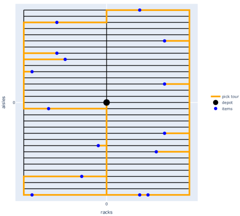
Figure 1: An illustration of a pick tour in a zone, where: the depot is located at the center (black dot), items are in aisles and rows (blue dots), and the orange line depicts the pick tour starting and ending at the depot.

An individual zone is composed of parallel aisles, with racks (shelves used for storing items) running along them, and a single depot (access point to the conveyor). Figure 1 shows an example pick tour. It is worth to note that any pick tour must be fully contained in a single zone, as well as begin and finish at that zone’s depot.

3 Problem definition

In this section, we formally define the Joint Order Selection, Allocation, Batching and Picking Problem by first describing the input data and then giving a problem definition.

Broadly speaking, we are given a set of customer orders and a warehouse containing available items. Each customer order consists of a set of articles (possibly containing duplicates). We are guaranteed that there are enough items in the warehouse to satisfy all customer orders. As mentioned before, the warehouse is divided into zones and each item in the warehouse is located in one of these zones. Together with the zone information, the location of a warehouse item is described by rack and aisle number. There could be multiple items stored at the same location (One can think of a box full of T-Shirts, for example). Each warehouse zone is assumed to have exactly one conveyor station (which corresponds to a depot), which is the place where warehouse workers pick up and drop off containers. Hence, a pick tour consists of a warehouse worker picking up a container at the conveyor station, picking all items on the picklist, and returning the full container to the conveyor station. The distance between two locations $x$ and $y$ is denoted by $d(x,y)$, which is only defined for two locations in the same zone. Additionally, there are three types of constraints that our solution should satisfy: a minimum total number of batched items, a maximum volume for articles in a picklist and a maximal number of orders in a batch. An overview on the input is given in Table 1.

name	symbol	description
Articles	${\mathcal{A}}$	Each article $a\in{\mathcal{A}}$ has a volume $vol(a)\in\mathbb{R}_{>0}$.
Orders	$\mathcal{O}$	Each order $o\in\mathcal{O}$ is a (multi-)set of articles $\{a_{1},a_{2},\dots\}$
Zones	$\mathcal{Z}$	Set of zones
Locations	$\mathcal{L}\subseteq\mathcal{Z}\times\mathbb{Z}\times\mathbb{Z}$	A location $l\in\mathcal{L}$ is a triplet of zone, rack and aisle number.
Warehouse Items	$\mathcal{I}$	Each item $i\in\mathcal{I}$ has an article $art(i)\in{\mathcal{A}}$ and a location $loc(i)\in\mathcal{L}$.
Conveyor Stations	$\mathcal{C}$ $\subseteq\mathcal{L}$	a set of conveyor stations with exactly one conveyor station per zone $z$ denoted by $C_{z}$
Walking Distance	$d:\mathcal{L}\times\mathcal{L}\to\mathbb{R}_{\geq 0}$	For two locations $x,y$ the walking distance $d(x,y)$ is only defined if $x$ and $y$ are in the same zone.
Item Goal	$IG$ $\in\mathbb{N}$	minimum number of required items to be batched
Picklist Volume	$V$$\in\mathbb{R}_{>0}$	maximum sum of article volumes for a picklist
Orders per Batch	$Q$$\in\mathbb{N}$	maximum number of orders a batch can consist of

Table 1: Problem Input and Parameters

The overall goal of the Joint Order Selection, Allocation, Batching and Picking Problem is to choose a subset of orders $O\subseteq\mathcal{O}$ and to create picklists for them, which are then picked by the warehouse workers. As an objective function the overall length of all picklists should be minimized. We now define what a picklist is.

Definition 3.1.

A picklist $p=(p_{1},\dots,p_{|p|})$ consists of an ordered set of warehouse items $p_{i}\in\mathcal{I}$. All items of a picklist are required to belong to the same zone $z_{p}$. We define the cost of a picklist as

$$cost(p):=d(C_{z_{p}},loc(p_{1}))+\left(\sum_{i=1}^{|p|-1}d(loc(p_{i}),loc(p_{i+1}))\right)+d(loc(p_{|p|}),C_{z_{p}}),$$

where $C_{z_{p}}$ is the conveyor station for zone $z_{p}$.

Given the definition of a picklist, we can now state the Joint Order Selection, Allocation, Batching and Picking Problem.

Definition 3.2.

Given inputs from Table 1, we define the batching problem as

$$\min_{O\subseteq\mathcal{O},I\subseteq\mathcal{I}}\quad \sum_{b=1,...,B}\sum_{p\in P_{b}}cost(p)$$ (1)

s.t. $$O=\underset{b=1,\dots,B}{\dot{\bigcup}}O_{b}$$ (2)

$$I=\underset{b=1,\dots,B}{\dot{\bigcup}}\underset{p\in P_{b}}{\dot{\bigcup}}\{i\in p\} P_{b}$$ where is a set of picklists (3)

$$\underset{o\in O_{b}}{\bigsqcup}o=\underset{p\in P_{b}}{\bigsqcup}\{art(i)\;|\;i\in p\} \quad\forall b\in\{1,...,B\}$$ (4)

$$|\{loc(i)\;|\;i\in p\}|\leq 1 \quad\forall p\in P_{b},b\in\{1,...,B\}$$ (5)

$$\sum_{i\in p}vol(art(i))\leq V \quad\forall p\in P_{b},b\in\{1,...,B\}$$ (6)

$$|O_{b}|\leq Q \quad\forall b\in\{1,...,B\}$$ (7)

$$|I|\geq IG$$ (8)

with $\dot{\cup}$ defined as the disjoint union and $\sqcup$ as the multiset union. We call the tuple $(O_{b},P_{b})$ a batch and the set of all batches $\mathcal{B}$.

For a solution $\mathcal{B}$ and its corresponding selected items $I$ we define the picklist cost per item to be

$$\text{pcpi}(\mathcal{B},I):=\frac{\sum_{b=1,...,B}\sum_{p\in P_{b}}cost(p)}{|I|}$$ (picklist cost per item)

Starting from the top, we choose orders $O$ and warehouse items $I$. The orders are divided into orders for each batch $b$ via constraint (2) and the total number of resulting batches is denoted by $B$. For the chosen items $I$ we require in (3) that each item is contained in exactly one picklist and each picklist belongs to one of the $B$ sets of picklists $P_{b}$. We ensure that the numbers of articles from orders $O_{b}$ match to the items in picklists $P_{b}$ via constraints (4). For each picklist $p$ constraints (5) ensures that all picklists items are in the same zone. Constraints (6) guarantee that the container volume is not exceeded. Constraints (7) ensure that the number of orders in a batch does not exceed the maximum orders per batch parameter $Q$. Finally, constraint (8) ensures that enough items are chosen to satisfy the item goal $IG$.

4 Baseline Solution Algorithms

While the main purpose of this work is to provide a thorough introduction to the Joint Order Selection, Allocation, Batching and Picking Problem, we also want to present baseline solution algorithms. The goal for these algorithms is not to solve the Joint Order Selection, Allocation, Batching and Picking Problem in the best possible way, but to provide an easy-to-understand entry point for the reader on how a possible solution algorithm could look like. In this section we propose two algorithms: The Distance Greedy Algorithm (DGA) (Algorithm 1) and a simplified version of it, which we call Randomized Distance Greedy Algorithm (RDGA).

DGA, given an instance of the Joint Order Selection, Allocation, Batching and Picking Problem, gradually computes batches $\mathcal{B}$ until either the item goal is reached or there are no more orders left in $\mathcal{O}$ to be processed. To compute a batch, the algorithm starts with an initially empty set of orders and one by one adds a new order to it together with a set of selected items. The order is chosen in a way that the corresponding selected items minimize the distance to already selected items (Function best_order), which is averaged by the number of the selected items. Orders are added to the set until the stopping criterion is reached, meaning that the number of order per batch has been reached or there are no orders left. Once this stopping criterion is met, the selected items of the batch are grouped in their zones and split into picklists. This is done heuristically: The items are sorted by their aisle number and then clustered together into picklists. The pseudocode is presented in Algorithm 1.

Data: as per Table 1

1 $\mathcal{B}\leftarrow\emptyset$

2 while $IG>0\;\text{and}\;\mathcal{O}\neq\emptyset$ do

3       $(\textit{O},\mathcal{S})\leftarrow(\emptyset,\emptyset)$

4       while $|\textit{O}|<Q\;\text{and}\;\mathcal{O}\neq\emptyset\;\text{and}\;|\mathcal{S}|<IG$ do

5             $(o,s)\leftarrow\texttt{best\_order}(\mathcal{O},\mathcal{S},\mathcal{I})$

6             $(\textit{O},\;\mathcal{O})\leftarrow(\textit{O}\cup\{o\},\;\mathcal{O}\setminus\{o\})$

7             $(\mathcal{S},\;\mathcal{I})\leftarrow(\mathcal{S}\cup s,\;\mathcal{I}\setminus s)$

8            

9      $\mathcal{P}\leftarrow\texttt{compute\_picklists}(\mathcal{S})$

10       $IG\leftarrow IG-|\mathcal{S}|$

11       $\mathcal{B}\leftarrow\mathcal{B}\cup\{(\textit{O},\mathcal{P})\}$

12return $\mathcal{B}$

13 Function best_order($\mathcal{O}$, $\mathcal{S}$, $\mathcal{I}$):

14       $(o^{*},s^{*},d^{*})\leftarrow(null,\emptyset,\infty)$

15       for $o\in\mathcal{O}$ do

16             $d\leftarrow 0$, $s\leftarrow\emptyset$

17             for $a\in o$ do

18                   $\textit{I}\leftarrow\{i\in\mathcal{I}\;|\;art(i)=a\}$

19                   $\mathcal{L}\leftarrow\{\text{loc}(j)\;|\;j\in s\cup\mathcal{S}\}\cup\mathcal{C}$

20                   $(d^{\prime},i^{\prime})\leftarrow\min\limits_{i\in\textit{I},j\in\mathcal{L}}(dist({\text{loc}(i)},{j}),i)$

21                   $(d,\;s)\leftarrow(d+d^{\prime},\;s\cup\{i^{\prime}\})$

22                  

23            if $\frac{d}{|s|}<\frac{d^{*}}{|s^{*}|}$ then

24                   $(o^{*},\;s^{*},\;d^{*})\leftarrow(o,\;s,\;d)$

25                  

26      return $(o^{*},s^{*})$

27 Function compute_picklists($\mathcal{S}$):

28       $\mathcal{P}\leftarrow\emptyset$

29       for $z\in\mathcal{Z}$ do

30             $\mathcal{I}_{z}\leftarrow\;\{i\in\mathcal{S}\;|\;\text{zone}({i})=z\}$

31             $p\leftarrow\emptyset$

32             for $i\in\text{sorted}(\mathcal{I}_{z},\text{key}=(i.aisle,i.rack))$ do

33                   if  $\textit{vol}(\text{art}({i}))+\sum_{j\in p}\textit{vol}(\text{art}({j}))\leq V$ then

34                         $p\leftarrow p\cup\{i\}$

35                        

36                  else

37                         $\mathcal{P}\leftarrow\mathcal{P}\cup p$

38                         $p\leftarrow\{i\}$

39                        

40            if $p\neq\emptyset$ then

41                   $\mathcal{P}\leftarrow\mathcal{P}\cup p$

42      return $\mathcal{P}$

Algorithm 1 Distance Greedy Algorithm

Lemma 4.1 (Complexity of DGA).

The complexity of Algorithm DGA is $O(|\mathcal{I}|^{3})$.

Proof.

Algorithm 1 makes at most $|\mathcal{I}|$ calls to best_order since every added order has at least one item and the total number of requested items $IG$ is not more than $|\mathcal{I}|$. Function best_order iterates through all requested articles of all remaining orders, which are in $O(|\mathcal{I}|)$. The minimum operator in best_order iterates over both $s$ and $\mathcal{L}$, which has complexity of $O(|\mathcal{I}|^{2})$. Finally, Function compute_picklists iterates through all items in a batch, for which there cannot be more than $|\mathcal{I}|$. The main complexity here is incurred by sorting, which is $O(|\mathcal{I}|log(|\mathcal{I}|)$. Hence, the complexity of this algorithm is dominated by calling Function best_order, which results in an overall complexity of $O(|\mathcal{I}|^{3})$. ∎

One can see that best_order dominates the complexity for DGA by computing several nested minima. Since this might be very time-consuming we introduce RDGA, that works by redefining best_order to

$$\texttt{best\_order}(\mathcal{O},\mathcal{S},\mathcal{I}):=\text{choose }o\in\mathcal{O}\text{ randomly}$$ (RDGA)

By doing so, we reduce the complexity of the algorithm from $O|\mathcal{I}|^{3})$ to $O(|\mathcal{I}|^{2})$. We will see in the Computational Experiments section how this significantly improves runtime, at the expense of a worse solution quality.

5 Experiments

In this section, we evaluate the performance of DGA and RDGA, for which we compare runtime and solution quality. We implemented both algorithms (DGA and RDGA) in Python 3.10 and made them available at https://github.com/zalandoresearch/batching-benchmarks/. Additionally, we published the set of instances we used in our experiments and the tool that created them.

Generation of Instances

We based the generation of instances on the problem definition in section 3 and on the following assumptions:

• Each zone in the warehouse is based on a two-dimensional grid, where one axis (the aisles) is freely walkable, and the second axis (the racks) is only walkable along the three cross-aisles. The layout is depicted in Figure 1.

• For each zone, there is exactly one depot (modeled as a single node) at coordinates $\text{rack}=0$ and $\text{aisle}=0$.

These assumptions aim at simplifying the instance format, while at the same time keeping the instances realistic.

We generated a total of 15 instances and divided them equally into three categories: small, medium and large. The categorization is based on the number of orders, items, zones as well as aisles and racks in each zone. Details about these parameters are summarized in Table 2. Individual instance details are given in Table 3.

Parameter (count)	Small	Medium	Large
Warehouse items	10,000	100,000	1,000,000
Orders	500	5,000	50,000
Zones	10	50	100
Racks	100	100	100
Aisles	100	100	100

Table 2: Parameters used for the generation of instances.

Category	Instance Name	total order articles	$IG$
small	small-0	1,322	264
	small-1	1,345	269
	small-2	1,312	262
	small-3	1,330	266
	small-4	1,325	265
medium	medium-0	13,115	2,623
	medium-1	13,223	2,644
	medium-2	13,135	2,627
	medium-3	13,236	2,647
	medium-4	13,135	2,625
large	large-0	131,873	26,374
	large-1	131,872	26,374
	large-2	131,827	26,365
	large-3	131,864	26,272
	large-4	132,092	26,418

Table 3: Details about each generated instance.

Analysis

We ran the experiments on a 2020 MacBook Pro with Apple M1 Chip (16GB RAM, 3.2GHz clock rate) on a single thread. The results are summarized in Tables 4 and  5, respectively. A comparison of the two tables shows that DGA yields better results in terms of optimization objective. On average, DGA-produced solutions are better than RDGA solutions by a factor of 2. This advantage of DGA, however, comes with the increased amount of computation times. More precisely, on large instances DGA can be up to $1500$ times slower than RDGA, which takes less than $10$ seconds (as opposed to $9941$ seconds, about 2.5 hours, in the case of DGA). From these observations it can be concluded that the DGA improves over RDGA but with the drawback of higher computation times.

Instances	Runtime (seconds)	Objective Value	Selected Items	Picklists	Batches
small-0	3	9,122	365	32	3
small-1	3	8,796	376	34	3
small-2	3	8,372	373	31	3
small-3	4	9,546	373	33	3
small-4	4	9,226	382	35	3
medium-0	113	66,602	2,687	872	23
medium-1	114	66,212	2,713	837	23
medium-2	114	65,320	2,667	847	23
medium-3	114	66,690	2,722	854	23
medium-4	112	65,668	2,665	865	23
large-0	9,972	606,478	26,405	10,842	231
large-1	10,062	607,618	26,434	10,830	231
large-2	9,927	600,110	26,419	10,810	231
large-3	9,955	607,246	26,375	10,840	231
large-4	9,941	610,202	26,440	10,907	230

Table 4: Results for DGA

Instances	Runtime (seconds)	Objective Value	Selected Items	Picklists	Batches
small-0	$<$1	9,814	265	20	2
small-1	$<$1	15,260	398	32	3
small-2	$<$1	10,782	269	20	2
small-3	$<$1	15,334	392	31	3
small-4	$<$1	9,996	273	22	2
medium-0	$<$1	141,752	2,726	951	21
medium-1	$<$1	141,932	2,743	971	21
medium-2	$<$1	137,050	2,634	900	20
medium-3	$<$1	135,246	2,653	905	20
medium-4	$<$1	136,742	2,660	897	20
large-0	7	1,494,408	26,420	14,134	201
large-1	7	1,489,980	26,430	14,236	201
large-2	7	1,493,316	26,401	14,255	201
large-3	7	1,495,004	26,296	14,123	200
large-4	7	1,497,366	26,454	14,203	201

Table 5: Results for RDGA

Impact of Order Selection

In a second experiment we investigated the impact of order selection on the overall batch quality. With the item goal $IG$ we defined the Joint Order Selection, Allocation, Batching and Picking Problem to choose a subset and not all of the commissions. It can be seen in Table 3 that we are only required to select roughly a fifth of all order items to satisfy the item goal. Now, we are asking, how does the solution change if we are not given this choice? To this end, we trimmed down the number of total order articles of the generated instances such that they exactly match the item goal. More precisely, we reduced the order pool of the input instance by randomly selecting orders until the total count of selected order items exceeded the item goal. For higher confidence in the results, we repeated this experiment five times for each instance and averaged the objective value of the solution. Hence, we created five different reduced order pools where the number of order articles equals $IG$ and reran DGA on them.

We summarize our findings in Table 6, where we compare the average picklist cost per item (pcpi) without order selection (modified instances) versus the previous original solutions.

Instances	pcpi modified instances	pcpi original instances	Difference
small-0	37.76	24.99	-34%
small-1	37.62	23.39	-38%
small-2	38.36	22.45	-41%
small-3	39.13	25.59	-35%
small-4	38.06	24.15	-37%
medium-0	42.31	24.79	-41%
medium-1	42.05	24.41	-42%
medium-2	42.28	24.49	-42%
medium-3	41.9	24.5	-42%
medium-4	41.87	24.64	-41%
large-0	39.07	22.97	-41%
large-1	39.14	22.99	-41%
large-2	39	22.72	-42%
large-3	39.13	23.02	-41%
large-4	39.05	23.08	-41%

Table 6: Total objective value normalized by number of chosen items

One can observe that the solutions to the new modified instances have a significantly higher pick cost per item, on average a $40\%$ better solution quality. Hence, we can conclude that the freedom to choose the orders, i.e. working with a requested number of items $IG$ leads to significantly better solution quality. In the literature it is often assumed that all available orders need to be batched (which is the case with the previously defined modified instances), but actually this is not necessarily required. For example, at Zalando the batching algorithms only need to compute batches such that the warehouse workers have work for the next 30 to 60 minutes, and hence many existing orders are not immediately batched. This insight from reality together with the computational results from above justify, or even necessitate, the use of an item goal $IG$.

6 Conclusion

In this work we presented the Joint Order Selection, Allocation, Batching and Picking Problem that models a central process of Zalando’s warehouse operations. We gave a formal problem definition and justified the need to integrate batching, item allocation and picker routing into one holistic problem. Furthermore, we explained the need to add an item goal – the minimum number of requested items – to the problem definition.

Algorithmically, we presented two baseline approaches to solve the Joint Order Selection, Allocation, Batching and Picking Problem. These algorithms intend to serve as a starting point for solving the problem and which can be used for comparisons with more sophisticated algorithms. The first algorithm, DGA, chooses the next order for a batch via a heuristic distance-based evaluation of all remaining orders. The second algorithm, RDGA, simplifies this approach even further by just selecting a random order as the next order to be added to a batch.

For the computational experiments, we generated a set of instances with parameters choosen to represent real-world applications. Algorithms, instances and the evaluation procedure were made publicly available. Based on our experimental results we concluded that the greedy algorithm clearly outperforms the randomized greedy at the cost of higher computation times. From the runtime explosion of DGA it is evident how difficult an implementation in reality is since the problem needs to be solved within a limited time frame in order to keep warehouse operations running. Beyond that, we could see in the second set of experiments that the introduction of an item goal $IG$ is key to improved solution quality.

One pertinent direction for future research involves presenting more sophisticated algorithms for the Joint Order Selection, Allocation, Batching and Picking Problem, which have to be designed around a careful trade-off between runtime and solution quality. Another promising direction involves analyzing the optimality gap of the presented solution algorithms. These can be found by lower bound computations as well as formulating exact approaches.

In general the intention of this publication is to give the interested reader a reasonably low entry barrier into real-world warehouse throughput optimization, in terms of problem complexity and presented baseline algorithms. Our hope is to make it convenient for other researchers to delve into this problem and we are looking forward to a fruitful exchange of ideas.

References

- BDKW [18] Nils Boysen, René De Koster, and Felix Weidinger. Warehousing in the e-commerce era: A survey. European Journal of Operational Research, 277, 08 2018.
- CVM+ [23] Giorgia Casella, Andrea Volpi, Roberto Montanari, Letizia Tebaldi, and Eleonora Bottani. Trends in order picking: a 2007–2022 review of the literature. Production & Manufacturing Research, 11(1):2191115, 2023.
- DKLDR [07] René De Koster, Tho Le-Duc, and Kees Jan Roodbergen. Design and control of warehouse order picking: A literature review. European journal of operational research, 182(2):481–501, 2007.
- DKLDZ [12] René De Koster, Tho Le Duc, and Nima Zaerpour. Determining the number of zones in a pick-and-sort order picking system. International Journal of Production Research, 50:757–771, 02 2012.
- DKP [98] René De Koster and Edo Poort. Routing orderpickers in a warehouse: A comparison between optimal and heuristic solutions. IIE Transactions, 30:469–480, 05 1998.
- DRS [98] Richard L. Daniels, Jeffrey L. Rummel, and Robert Schantz. A model for warehouse order picking. Eur. J. Oper. Res., 105:1–17, 1998.
- GvdV [05] Noud Gademann and Steef van de Velde. Order batching to minimize total travel time in a parallel-aisle warehouse. IIE Transactions, 37(1):63–75, 2005.
- Hal [93] Randolph W Hall. Distance approximations for routing manual pickers in a warehouse. IIE transactions, 25(4):76–87, 1993.
- HS [13] Sebastian Henn and Verena Schmid. Metaheuristics for order batching and sequencing in manual order picking systems. Computers & Industrial Engineering, 66(2):338–351, 2013.
- Int [23] Bowe Intralogistics. Sorters. https://bowe.com/intralogistics/en/p/sorters/, 2023. [Online; accessed 23-August-2023].
- OZD [17] Sevilay Onal, Jingran Zhang, and Sanchoy Das. Modelling and performance evaluation of explosive storage policies in internet fulfilment warehouses. International Journal of Production Research, 55:1–14, 03 2017.
- RR [83] H Donald Ratliff and Arnon S Rosenthal. Order-picking in a rectangular warehouse: a solvable case of the traveling salesman problem. Operations research, 31(3):507–521, 1983.
- SHSW [16] André Scholz, Sebastian Henn, Meike Stuhlmann, and Gerhard Wäscher. A new mathematical programming formulation for the single-picker routing problem. European Journal of Operational Research, 253(1):68–84, 2016.
- SSW [17] André Scholz, Daniel Schubert, and Gerhard Wäscher. Order picking with multiple pickers and due dates - simultaneous solution of order batching, batch assignment and sequencing, and picker routing problems. European Journal of Operational Research, 263, 04 2017.
- TBDR [10] Christophe Theys, Olli Bräysy, Wout Dullaert, and Birger Raa. Using a tsp heuristic for routing order pickers in warehouses. European Journal of Operational Research, 200(3):755–763, 2010.
- TWBT [10] J.A. Tompkins, J.A. White, Y.A. Bozer, and J.M.A. Tanchoco. Facilities Planning. Wiley, 2010.
- VBDC [17] Cristiano Arbex Valle, John E Beasley, and Alexandre Salles Da Cunha. Optimally solving the joint order batching and picker routing problem. European Journal of Operational Research, 262(3):817–834, 2017.
- vGCRB [19] Teun van Gils, An Caris, Katrien Ramaekers, and Kris Braekers. Formulating and solving the integrated batching, routing, and picker scheduling problem in a real-life spare parts warehouse. European Journal of Operational Research, 277, 03 2019.
- vGRCDK [18] Teun van Gils, Katrien Ramaekers, An Caris, and René De Koster. Designing efficient order picking systems by combining planning problems: State-of-the-art classification and review. European Journal of Operational Research, 267:1–15, 05 2018.
- Wäs [04] Gerhard Wäscher. Order Picking: A Survey of Planning Problems and Methods, pages 323–347. Springer Berlin Heidelberg, Berlin, Heidelberg, 2004.
- WBS [19] Felix Weidinger, Nils Boysen, and Michael Schneider. Picker routing in the mixed-shelves warehouses of e-commerce retailers. European Journal of Operational Research, 274(2):501–515, 2019.
- WO [05] J. Won and S. Olafsson. Joint order batching and order picking in warehouse operations. International Journal of Production Research, 43(7):1427–1442, 2005.
- XLL [22] Lin Xie, Hanyi Li, and Laurin Luttmann. Formulating and solving integrated order batching and routing in multi-depot agv-assisted mixed-shelves warehouses. European Journal of Operational Research, 307, 09 2022.
- YZG [20] Peng Yang, Zhijie Zhao, and Huijie Guo. Order batch picking optimization under different storage scenarios for e-commerce warehouses. Transportation Research Part E: Logistics and Transportation Review, 136:101897, 2020.
- ZWG [21] Minqi Zhang, Sven Winkelhaus, and Eric H. Grosse. Evaluation of human workload in a hybrid order picking system. IFAC-PapersOnLine, 54(1):458–463, 2021. 17th IFAC Symposium on Information Control Problems in Manufacturing INCOM 2021.