LASPATED: a Library for the Analysis of SPAtio-TEmporal Discrete data

Abstract

We describe methods, tools, and a software library called LASPATED, available on GitHub to fit models using spatio-temporal data and space-time discretization. A video tutorial for this library is available on YouTube. We consider two types of methods to estimate a non-homogeneous Poisson process in space and time. The methods approximate the arrival intensity function of the Poisson process by discretizing space and time, and estimating arrival intensity as a function of subregion and time interval. With such methods, it is typical that the dimension of the estimator is large relative to the amount of data, and therefore the performance of the estimator can be improved by using additional data. The first method uses additional data to add a regularization term to the likelihood function for calibrating the intensity of the Poisson process. The second method uses additional data to estimate arrival intensity as a function of covariates. We describe a Python package to perform various types of space and time discretization. We also describe two packages for the calibration of the models, one in Matlab and one in C++. We demonstrate the advantages of our methods compared to basic maximum likelihood estimation with simulated and real data. The experiments with real data calibrate models of the arrival process of emergencies to be handled by the Rio de Janeiro emergency medical service.

Vincent Guigues School of Applied Mathematics, FGV Praia de Botafogo, Rio de Janeiro, Brazil vincent.guigues@fgv.br

Anton J. Kleywegt Georgia Institute of Technology Atlanta, Georgia 30332-0205, USA anton@isye.gatech.edu

Giovanni Amorim School of Applied Mathematics, FGV Praia de Botafogo, Rio de Janeiro, Brazil giovanni.argento100@gmail.com

André Mazal Krauss Department of Informatics, PUC-RJ Rio de Janeiro, Rio de Janeiro, Brazil amk1710@gmail.com

Victor Hugo Nascimento

Systems Engineering and Computer Science, UFRJ

Cidade Universitária, Rio de Janeiro, Brazil

victorrn@cos.ufrj.br

Keywords: Poisson process, spatio-temporal discretization, mathematical software, library, discrete data, emergency health services.

1 Introduction

In many applications, one would like to use data to fit a function such as $f:\mathcal{S}\times[0,T]\mapsto\mathbb{R}$, where $\mathcal{S}$ is a bounded subset of $\mathbb{R}^{n}$. Often, the domain $\mathcal{S}$ is called “space” and the domain $[0,T]$ is called “time”. For example, $\mathcal{S}$ may represent locations on a $2$-dimensional map (in which case $n=2$), or locations in a $3$-dimensional space (in which case $n=3$), or origin-destination pairs on a map (in which case $n=4$), and $[0,T]$ may represent time of the day (in which case $T=24$ hours), or time of the week (in which case $T=168$ hours).

A widely used non-parametric approach for fitting such a function $f$ with data is to discretize space and time in a way that may depend on the data, and to fit a function from a chosen class on each discrete subset of the domain. There are many ways to choose such discretization. For example, the fitted function may be piecewise constant, that is, it may be constant on each discrete subset of the domain and there are benefits to allowing the discretization to depend on the data. For example, a finer discretization may be chosen in regions of space and time with a higher concentration of data.

Furthermore, sometimes one has data of covariates on the same space-time domain, with the covariates being correlated with the dependent variable. Even if the main purpose of the study is not to model the relation between the dependent variable and the covariates, these covariate data can be used in various ways to improve the estimates. For example, the covariates can be used in the choice of discretization, for example, by choosing the subsets of the discretization to be relatively uniform in terms of the covariate values. The covariates can also be used as auxiliary independent variables in the fitted model. The covariates can also be used to regularize the parameter estimates, especially when data are sparse.

Software tools for managing the choice of discretization, the regularization, and the parameter estimation, can be of great use. This paper describes a collection of such software tools for function estimation with spatio-temporal data.

1.1 Application

Next, we describe the application that motivated the development of these software tools, and that will also be used in this paper to demonstrate the use of these tools. Phone calls about medical emergencies arrive at a call center for emergency medical services (EMSs). Each emergency is characterized by a type, a location, and the arrival time of the call. The type of emergency is determined by the classification system used by the EMS, such as the Medical Priority Dispatch System (MPDS) or the Association of Public-Safety Communications Officials (APCO) system. Typical classification systems classify emergencies by the anatomical region (e.g., chest) affected, the cause of the emergency (e.g., animal bites), the importance of response time (e.g., “hot” versus “cold”), and the level of emergency service needed (e.g., basic life support versus advanced life support). The location is typically specified by an address, but can be converted to a latitude-longitude coordinate. The arrival time of the call is specified by a date-time combination.

We would like to estimate the arrival rate of emergencies as a function of emergency type, location, and time. Such an arrival rate function can be used to optimize the types and number of ambulances needed, the types and number of crew members needed, the crew schedules, and the positioning and dispatch of ambulances, and to develop a simulation of the emergency response system. We consider methods that discretize space and time and then estimate the arrival rate as a function of discrete space and time. While working on such a project (see [1]), we identified the lack of easy-to-use tools for this type of analysis. Thus, the LASPATED library was created as a general tool to fill this gap.

1.2 Overview of the LASPATED Library

Various space and time discretizations were implemented in LASPATED to partition space and time data. LASPATED facilitates four types of space discretization: in rectangles, in hexagons, based on the Voronoi diagram for a set of points in $\mathcal{S}$, and customized discretizations. LASPATED also provides functions to combine information from two different space discretizations, such as functions to calculate the areas of intersection of pairs of subregions from two discretizations, or to calculate location data such as population in the intersection of pairs of subregions from two discretizations.

LASPATED also facilitates various types of time discretization. For example, a simple partitioning of time could be a partition of the week in time intervals of $1$ hour each. Then the corresponding time intervals are $\left\{\mbox{Monday[0:00,1:00)},\mbox{Monday[1:00,2:00)},\mbox{Monday[2:00,3:00)},\ldots,\mbox{Sunday[23:00,24:00)}\right\}$. Time intervals of different types can also be distinguished. For example, there could be different time intervals such as Monday[0:00,1:00) for different holidays, or there could be different time intervals such as Friday[20:00,21:00) depending on the scheduling of a sport event at the time. For instance, for the time window Friday[20:30,21:00), one could have

• a time interval for Friday [20:30,21:00) on days which are holidays and a major sport event is scheduled;

• a time interval for Friday [20:30,21:00) on days which are holidays and a major sport event is not scheduled;

• a time interval for Friday [20:30,21:00) on days which are not holidays and a major sport event is scheduled; and

• a time interval for Friday [20:30,21:00) on days which are not holidays and a major sport event is not scheduled.

Given a point in space $\ell_{0}\in\mathcal{S}$ and time $t_{0}\in[0,T]$, possibly with additional characteristics such as holiday or event type, LASPATED determines the spatial subregion and the time interval for the chosen discretization that contains the given point. Furthermore, given a data set of observations, each consisting of several points, LASPATED computes the number of points in the data set in each combination of spatial subregion and time interval for the chosen discretization, for each observation. For example, given a data set of medical emergencies, with a week of data associated with each observation, LASPATED computes the number of emergencies in the data set for each combination of type of emergency, spatial subregion, and time interval, for the chosen discretization, for each week of data.

LASPATED also facilitates calibration of models using discrete spatio-temporal data prepared with the discretization subroutines. For example, suppose that the number of points of a point process is Poisson with intensity that is a function of type, spatial location, and time, and that a piecewise constant arrival rate model $\lambda_{c,i,t}$ for type $c$, spatial subregion $i$, and time interval $t$, is estimated. LASPATED provides two approaches discussed in Section 2 to calibrate these piecewise constant intensities. Both approaches allow one to deal with sparse data, for example when there are many combinations of subregion and time window in the discretization relative to the amount of data. In the first approach, the intensities are the solutions of an optimization problem which optimizes a linear combination of the log-likelihood and a regularization term that may include covariates or penalize non-smoothness of intensities regarding space and time. For the second approach, covariates are used as auxiliary explanatory variables in the model.

The outline of the paper is as follows. In Section 2, we describe models to be estimated with discretized spatio-temporal data, and explain how the parameters of these models can be calibrated, making provision for cases in which relatively little data are available. Time discretization functionalities are described in Section 3. Space discretization is discussed in Sections 4 and 5. LASPATED model calibration functionalities are described in Section 6. A detailed description of each function is provided in the LASPATED user manual. The user manual [3] also shows how to use LASPATED functions for some examples. The user can also learn how to use LASPATED with an online video tutorial. In Section 7, we demonstrate our estimators of Poisson intensities, and we compare the results with basic maximum likelihood estimators, using numerical experiments with simulated data. We also demonstrate the use of LASPATED to calibrate models of the arrival process of emergency calls to the Rio de Janeiro emergency medical service.

2 Statistical Models with Discretized Spatio-Temporal Data

In this section, we describe the models that motivated the work on LASPATED, and we explain how LASPATED solves the optimization problems for the calibration of these models. We will use the medical emergency application as a running example to explain the models.

Let $\mathcal{I}$ denote the subsets of the space discretization forming a partition of the region $\mathcal{S}\subset\mathbb{R}^{n}$; the elements of $\mathcal{I}$ will be called zones. Let $\mathcal{T}$ denote the subsets of the time discretization forming a partition of all times of interest; the elements of $\mathcal{T}$ will be called time intervals. Let $\mathcal{C}$ denote the set of point types; $\mathcal{C}$ can be any finite set that forms a partition of all space-time points of interest; the elements of $\mathcal{C}$ will be called types.

2.1 Model without Covariates

Each time interval $t\in\mathcal{T}$ has a duration $\mathcal{D}_{t}$ (in time units). It is assumed that data are observed for multiple occurrences of the same time interval $t$, and that each time data are observed for a type $c\in\mathcal{C}$, zone $i\in\mathcal{I}$, and time interval $t\in\mathcal{T}$, all such space-time points in the same time interval are recorded in the data. For example, suppose that $\mathcal{T}$ forms a partition of the week in time intervals of $1$ hour each. Then it is assumed that the data contain observations of emergencies of type $c$ in zone $i$ during hour $t\in\mathcal{T}$ for multiple weeks, and that each time emergency arrivals of type $c$ in zone $i$ are observed during a particular hour $t$ of a particular week, all the emergency arrivals of the same type in the same zone during the same hour $t$ of that week are recorded. (It is planned to make provision for censored data in future work.) All the emergency arrivals of a particular type $c$ in a particular zone $i$ during a particular hour $t$ of a week together are called an observation. For each $c\in\mathcal{C}$, $i\in\mathcal{I}$, and $t\in\mathcal{T}$, let $N_{c,i,t}$ denote the number of observations for type $c$, zone $i$, and time interval $t$, and let these observations be indexed by $n\in\mathcal{N}_{c,i,t}\vcentcolon=\{1,\ldots,N_{c,i,t}\}$. For each $c\in\mathcal{C}$, $i\in\mathcal{I}$, $t\in\mathcal{T}$, and $n\in\mathcal{N}_{c,i,t}$, let $M_{c,i,t,n}$ denote the number of points (arrivals) for observation $n$ of type $c$, zone $i$, and time interval $t$, and let $M_{c,i,t}\vcentcolon=\sum_{n=1}^{N_{c,i,t}}M_{c,i,t,n}$ denote the total number of points over all observations for type $c$, zone $i$, and time interval $t$.

Assume that $\big{\{}M_{c,i,t,n},c\in\mathcal{C},i\in\mathcal{I},t\in\mathcal{T},n\in\mathcal{N}_{c,i,t}\big{\}}$ are independent (but not necessarily identical) Poisson distributed random variables. Let $\lambda_{c,i,t}$ denote the mean number of points per length of time (such as per hour) for type $c$, zone $i$, and time interval $t$. Then random variable $M_{c,i,t,n}$ is Poisson distributed with mean $\lambda_{c,i,t}\mathcal{D}_{t}$. Let $\lambda\vcentcolon=\big{(}\lambda_{c,i,t},c\in\mathcal{C},i\in\mathcal{I},t\in\mathcal{T}\big{)}$. Then the likelihood function is

$$L(\lambda)\ \ =\ \ \prod_{c\in\mathcal{C}}\prod_{i\in\mathcal{I}}\prod_{t\in\mathcal{T}}\prod_{n\in\mathcal{N}_{c,i,t}}e^{-\lambda_{c,i,t}\mathcal{D}_{t}}\frac{(\lambda_{c,i,t}\mathcal{D}_{t})^{M_{c,i,t,n}}}{M_{c,i,t,n}!}$$

and intensities $\lambda$ that maximize the log-likelihood are the same intensities that solve

$$\min_{\lambda}\left\{\mathscr{L}(\lambda)\ \ \vcentcolon=\ \ \sum_{c\in\mathcal{C}}\sum_{i\in\mathcal{I}}\sum_{t\in\mathcal{T}}\left[N_{c,i,t}\lambda_{c,i,t}\mathcal{D}_{t}-M_{c,i,t}\log\left(\lambda_{c,i,t}\right)\right]\right\}.$$ (1)

A typical issue with such applications is that the distribution of data is far from uniform — there are a few combinations of type $c$, zone $i$, and time interval $t$ with many observations, but for most combinations of type $c$, zone $i$, and time interval $t$ there are very few observations. In such cases, it may be advantageous to use data from “neighboring” observations, or to bring additional data to bear on the estimation problem. For example, suppose that $\mathcal{T}$ forms a partition of the week in time intervals of $1$ hour each, but that it is expected that many hours of the week are similar to other hours of the week in terms of arrival rates. A simple approach to incorporate such an idea is to partition $\mathcal{T}$ into a collection $\mathcal{G}$ of subsets of $\mathcal{T}$ in such a way that it may be reasonable to expect that, for each $c\in\mathcal{C}$, $i\in\mathcal{I}$, and $G\in\mathcal{G}$, the values of $\lambda_{c,i,t}$ for different $t\in G$ will be close to each other (but not necessarily the same). Let $W_{G}\geq 0$ denote a similarity weight for $G\in\mathcal{G}$. Another approach to incorporate such an idea is to specify a similarity weight $w_{t,t^{\prime}}\geq 0$ for each (unordered) pair $t,t^{\prime}\in\mathcal{T}$. For example, $w_{t,t^{\prime}}=w>0$ if $t$ and $t^{\prime}$ are neighboring time intervals, and $w_{t,t^{\prime}}=0$ otherwise. Similarly, it may be expected that many zones are similar to other zones in terms of arrival rates. Such an idea can also be incorporated by partitioning the set $\mathcal{I}$ of zones into subsets, each with its own similarity weight, or by specifying for each pair $i,j\in\mathcal{I}$, a similarity weight $w_{i,j}\geq 0$. An example loss function with similarity regularization that uses the first approach for time intervals and the second approach for zones is given by

$$\begin{array}[]{lcl}\ell(\lambda)&=&\displaystyle\sum_{c\in\mathcal{C}}\sum_{i\in\mathcal{I}}\sum_{G\in\mathcal{G}}\sum_{t\in G}\left[N_{c,i,t}\lambda_{c,i,t}\mathcal{D}_{t}-M_{c,i,t}\log\left(\lambda_{c,i,t}\right)+\frac{W_{G}}{2}\sum_{t^{\prime}\in G}N_{c,i,t}N_{c,i,t^{\prime}}\left(\lambda_{c,i,t}-\lambda_{c,i,t^{\prime}}\right)^{2}\right]\\ &&\displaystyle+\sum_{c\in\mathcal{C}}\sum_{i,j\in\mathcal{I}}\sum_{t\in\mathcal{T}}\frac{w_{i,j}}{2}N_{c,i,t}N_{c,j,t}\left(\lambda_{c,i,t}-\lambda_{c,j,t}\right)^{2}.\end{array}$$ (2)

Intensity estimates $\lambda$ are then obtained by solving

$$\min_{\lambda>0}\;\ell(\lambda).$$ (3)

2.2 Model with Covariates

Each type $c$, zone $i$, and time interval $t$ may have covariates that are correlated with the arrival rates $\lambda_{c,i,t}$, and data of these covariates can be used to partly compensate for sparse data. For example, emergency arrival rates in different zones and time intervals can be expected to be correlated with the population and other measures of economic activity in the zones, as well as with festivals and other events during the time intervals. For each $c\in\mathcal{C}$, $i\in\mathcal{I}$, and $t\in\mathcal{T}$, let $x_{c,i,t}\vcentcolon=(x_{c,i,t,1},\ldots,x_{c,i,t,K})$ be the covariate values of type $c$, zone $i$, and time interval $t$. For example, $x_{c,i,t,1}$ may be the population count with home addresses in a zone $i$, and $x_{c,i,t,2}$ may be an indicator that a major sports event is scheduled in zone $i$ during time interval $t$. Then consider the model

$$\lambda(x_{c,i,t})\mathcal{D}_{t}\ \ =\ \ \beta^{\top}x_{c,i,t}$$ (4)

where $\beta=(\beta_{1},\ldots,\beta_{K})$ are the model parameters. Let $\mathcal{X}_{c,i,t}$ denote the set of all possible values of $x_{c,i,t}$. Often $\mathcal{X}_{c,i,t}$ can be chosen to be a polyhedron. Note that it should hold that

$$\beta^{\top}x_{c,i,t}\ \ \geq\ \ 0\qquad\forall\ x_{c,i,t}\in\mathcal{X}_{c,i,t},\ \forall\ c\in\mathcal{C},i\in\mathcal{I},t\in\mathcal{T}.$$ (5)

To facilitate such a model, let $N=\sum_{c\in\mathcal{C}}\sum_{i\in\mathcal{I}}\sum_{t\in\mathcal{T}}N_{c,i,t}$ denote the total number of observations, and let these observations be indexed $n=1,\ldots,N$. For each observation $n\in\{1,\ldots,N\}$, let $M_{n}$ denote the number of arrival points for observation $n$ and let $x^{n}\vcentcolon=(x^{n}_{1},\ldots,x^{n}_{K})$ denote the covariate values of observation $n$. Then the negative log-likelihood function is given by

$$\mathscr{L}(\beta)\ \ =\ \ \sum_{n=1}^{N}\left[\beta^{\top}x^{n}-M_{n}\log\left(\beta^{\top}x^{n}\right)\right].$$ (6)

Next we provide two examples of such models.

Example 2.1.

Index $\mathcal{C}=\{1,\ldots,|\mathcal{C}|\}$, $\mathcal{T}=\{1,\ldots,|\mathcal{T}|\}$, and let $K_{1}\vcentcolon=|\mathcal{C}\times\mathcal{T}|$. For each $c\in\mathcal{C}$, $t\in\mathcal{T}$, and $k=(c-1)|\mathcal{T}|+t$, let $x^{n}_{k}$ be the number of people resident (population count) in the zone of observation $n$ if observation $n$ is for type $c$ and time interval $t$, and $x^{n}_{k}=0$ otherwise. The next covariate is a set of occupational land use areas (in km²), for instance the areas of commercial activities and public facilities, of industrial activities, and of undeveloped land. Index the occupational land uses by $\mathcal{O}=\{1,\ldots,|\mathcal{O}|\}$. For each $c\in\mathcal{C}$, $t\in\mathcal{T}$, $m\in\mathcal{O}$, and $k=K_{1}+(c-1)|\mathcal{T}||\mathcal{O}|+(t-1)|\mathcal{O}|+m$, let $x^{n}_{k}$ be the area of occupational land use $m$ in the zone of observation $n$ if observation $n$ is for type $c$ and time interval $t$, and $x^{n}_{k}=0$ otherwise. Then $\sum_{k=1}^{K_{1}}\beta_{k}x^{n}_{k}$ denotes the forecasted number of arrivals for the type of observation $n$ in the zone of observation $n$ during the time interval of observation $n$ due to people being in the residential area, which is modeled as proportional to the number of people resident in the zone of observation $n$ with a proportionality coefficient that depends on the type and the time interval. Similarly, $\sum_{k=K_{1}+1}^{K_{1}(1+|\mathcal{O}|)}\beta_{k}x^{n}_{k}$ denotes the forecasted number of arrivals for the type of observation $n$ in the zone of observation $n$ during the time interval of observation $n$ due to people being in the different occupational areas which is modeled as proportional to the areas of occupational land use in the zone of observation $n$ with a proportionality coefficient that depends on the type and the time interval. If $K_{1}|\mathcal{O}|$ is large, the number of parameters $\beta_{k}$ of the model specified in this example is also large. Similar to (2), similarity regularization can be used to estimate the parameters, for example, by minimizing a loss function such as

$$\ell(\beta)\ \ =\ \ \sum_{n=1}^{N}\left[\beta^{\top}x^{n}-M_{n}\log\left(\beta^{\top}x^{n}\right)\right]+\sum_{k,k^{\prime}=1}^{K_{1}(1+|\mathcal{O}|)}\frac{w_{k,k^{\prime}}}{2}\left(\beta_{k}-\beta_{k^{\prime}}\right)^{2}.$$

Example 2.2.

This example will be used to demonstrate the modeling of arrivals of emergency calls to an emergency medical service. The sets $\mathcal{C}$, $\mathcal{I}$, and $\mathcal{O}$ are the same as in Example 2.1. Let $\mathcal{T}$ denote the indices of discrete time periods during a day, for example, $\mathcal{T}=\{1,\ldots,48\}$ if each day is discretized into $30$-minute intervals. Let $\mathcal{D}$ denote the set of indices of the (normal) days of the week as well as indices for special days. Thus, the cardinality of $\mathcal{D}$ is 7 plus the number of special days. A pair $(d,t)\in\mathcal{D}\times\mathcal{T}$ specifies a time interval. For each zone $i\in\mathcal{I}$, consider covariates $x_{i}\in\mathbb{R}^{1+|\mathcal{O}|}$, where $x_{i}(1)$ is the population count in zone $i$, and $x_{i}(j+1)$ is the area (in km²) of occupational land use $j$ in zone $i$ for $j=1,\ldots,|\mathcal{O}|$. Here we assume that these data (population and land type areas) do not depend on time, which is reasonable for moderate time periods. Then, for each type $c$, zone $i$, day $d$, and time period $t$, the arrival intensity is given by $\lambda_{c,i,d,t}\mathcal{D}_{t}=\beta_{c,d,t}^{\top}x_{i}$ for some vector $\beta_{c,d,t}\in\mathbb{R}^{1+|\mathcal{O}|}$). Furthermore, for each type $c$, zone $i$, day $d$, and time period $t$, let $N_{c,i,d,t}$ denote the number of observations, let $M_{c,i,d,t,n}$ denote the number of arrival points for observation $n$, and let $M_{c,i,d,t}\vcentcolon=\sum_{n=1}^{N_{c,i,d,t}}M_{c,i,d,t,n}$. Then the negative of the log-likelihood function is given by

$$\begin{array}[]{rl}\mathscr{L}(\beta)&=\ \ \displaystyle\sum_{c\in\mathcal{C}}\sum_{i\in\mathcal{I}}\sum_{d\in\mathcal{D}}\sum_{t\in\mathcal{T}}\sum_{n=1}^{N_{c,i,d,t}}\left[\beta_{c,d,t}^{\top}x_{i}-M_{c,i,d,t,n}\log(\beta_{c,d,t}^{\top}x_{i})\right]\\ &=\ \ \displaystyle\sum_{c\in\mathcal{C}}\sum_{i\in\mathcal{I}}\sum_{d\in\mathcal{D}}\sum_{t\in\mathcal{T}}\left[N_{c,i,d,t}\beta_{c,d,t}^{\top}x_{i}-M_{c,i,d,t}\log(\beta_{c,d,t}^{\top}x_{i})\right].\end{array}$$ (7)

Note that call rates $\beta_{c,d,t}^{\top}x_{i}$ should be positive. Additionally, for each type $c$, day $d$, and time period $t$, the coefficients $\beta_{c,d,t}(1)$ that represent the ratio of emergencies to population should be small (say less than 1), which implies the constraints $0\leq\beta_{c,d,t}(1)\leq 1$. Therefore, the estimation problem is to solve the optimization problem

$$\begin{array}[]{rl}\min&\ \ \mathscr{L}(\beta)\\ \mbox{s.t.}&\ \ \beta_{c,d,t}^{\top}x_{i}\ >\ 0,\quad 0\ \leq\ \beta_{c,d,t}(1)\ \leq\ 1,\qquad\forall\ c\in\mathcal{C},d\in\mathcal{D},t\in\mathcal{T}.\end{array}$$ (8)

Depending on the solver, better numerical performance may be obtained by replacing the constraints of (8) with

$$\beta_{c,d,t}^{\top}x_{i}\ \geq\ \varepsilon,\quad 0\ \leq\ \beta_{c,d,t}(1)\ \leq\ 1,\qquad\forall\ c\in\mathcal{C},d\in\mathcal{D},t\in\mathcal{T},$$ (9)

for some $\varepsilon>0$ sufficiently small.

2.3 Solving the Optimization Problems

The calibration of models such as those of Section 2.1 requires solving an optimization problem (3) of the form $\min\{\ell(\lambda)\,:\,\lambda>0\}$. The problem can also be formulated as

$$\min\;\{\ell(\lambda)\;:\;\lambda\in C\}$$ (10)

where $C$ is a closed convex set such as

$$C\ \ =\ \ \{\lambda\;:\;\lambda\geq\varepsilon\textbf{e}\}$$ (11)

for $\varepsilon>0$ sufficiently small and e a vector of ones. The objective function $\ell$ of (10) is differentiable on such $C$.

Problem (8) can be written as

$$\min\;\{\mathscr{L}(\beta)\;:\;\beta\in B\}$$ (12)

where $B$ is given by (9). In both cases, the problem is a convex optimization problem with a differentiable objective function on the feasible set.

Projected gradient with line search.

LASPATED solves problems (10) and (12) using a projected gradient method with line search along a feasible direction, as given in [2]. Another (usually slower) variant of the projected gradient method to solve such problems, namely a projected gradient method with line search along the boundary, is also provided in the LASPATED library. These variants follow [2] except for the choice of $\Delta$ for the variant with Armijo search along the feasible direction. Here, we provide the pseudocode of these variants for a problem of form (10). $\Pi_{C}(\lambda)$ denotes the projection of $\lambda$ onto closed convex set $C$. The pseudocode presents methods that are run for a given number of iterations and that start from any feasible $\lambda_{0}\in C$. For alternative stopping criteria, see the discussion at the end of this section.

 

Projected gradient method with Armijo search along a feasible direction for convex problem (10).  

Initialization: Choose $\sigma\in(0,1)$, $b>0$, MaxNumberIteration $>0$, and a feasible initial value $\lambda_{0}\in C$

// MaxNumberIteration is the maximum number of iterations

$\lambda=\lambda_{0}$

$k=1$ // $k$ is the iteration count

While $k\leq$ MaxNumberIteration

If ($k=1$)

$\Delta=\bar{\Delta}$

else

$\displaystyle\Delta=\bar{\Delta}/2^{j}$

End If

Compute $\ell(\lambda)$ and $\nabla\ell(\lambda)$

$z=\Pi_{C}(\lambda-\Delta\nabla\ell(\lambda))$

continue $=1$, $j=0$

While (continue)

$\displaystyle\mbox{zAux}=\lambda+(1/2^{j})(z-\lambda)$                  (a)

Compute $\ell(\mbox{zAux})$.

If $\displaystyle{\ell(\mbox{zAux})\leq\ell(\lambda)+\frac{\sigma}{2^{j}}\nabla\ell(\lambda)^{\top}(z-\lambda)}$

continue $=0$

else

$j\leftarrow j+1$

End If

End While

$\displaystyle\lambda=\mbox{zAux}$

$k\leftarrow k+1$

End While  

 

Projected gradient with Armijo search along the boundary for convex problem (10).   The pseudocode below presents the projected gradient method with line search along the boundary.  

Initialization: Choose $\sigma\in(0,1)$, $\bar{\Delta}>0$, MaxNumberIteration $>0$, and a feasible initial value $\lambda_{0}\in C$

// MaxNumberIteration is the maximum number of iterations

$\lambda=\lambda_{0}$

$k=1$

While $k\leq$ MaxNumberIteration

Compute $\ell(\lambda)$ and $\nabla\ell(\lambda)$

continue $=1$, $j=0$

While (continue)

$\displaystyle z=\Pi_{C}(\lambda-(\bar{\Delta}/2^{j})\nabla\ell(\lambda))$

Compute $\ell(\mbox{z})$

If $\displaystyle\ell(z)\leq\ell(\lambda)+\sigma\nabla\ell(\lambda)^{\top}(z-\lambda)$

continue $=0$

else

$j\leftarrow j+1$

End If

End While

$\lambda=z$

$k\leftarrow k+1$

End While  

Note that for problem (10) with $C=\{\lambda\,:\,\lambda\geq\varepsilon\textbf{e}\}$, the projection $\Pi_{C}(\lambda)=\max\{\lambda,\varepsilon\textbf{e}\}$ onto $C$ is easy to compute, where the max is taken componentwise. Furthermore, the derivative of $\ell$ is given by

$$\frac{\partial\ell(\lambda)}{\partial\lambda_{c,i,t}}\ \ =\ \ N_{c,i,t}\mathcal{D}_{t}-\frac{M_{c,i,t}}{\lambda_{c,i,t}}+W_{G(t)}\sum_{t^{\prime}\in G(t)}(\lambda_{c,i,t}-\lambda_{c,i,t^{\prime}})+\sum_{j\in\mathcal{I}}w_{i,j}(\lambda_{c,i,t}-\lambda_{c,j,t}),$$

where $G(t)$ is the group of time intervals to which $t$ belongs. For problem (12), the gradient of $\mathscr{L}$ is given by

$$\frac{\partial\mathscr{L}(\beta)}{\partial\beta_{c,d,t}}\ \ =\ \ \sum_{i\in\mathcal{I}}\left[N_{c,i,d,t}x_{i}-\frac{M_{c,i,d,t}x_{i}}{\beta_{c,d,t}^{\top}x_{i}}\right].$$

For problem (12) with $B=\left\{\beta\,:\,\beta_{c,d,t}^{\top}x_{i}\geq\varepsilon,\,0\leq\beta_{c,d,t}(1)\leq 1,\,\forall\;c\in\mathcal{C},d\in\mathcal{D},t\in\mathcal{T}\right\}$, the projection $\Pi_{B}(\beta)$ onto $B$ is computed by solving a convex quadratic problem.

Stopping test for projected gradient method with line search.

LASPATED makes provision for several stopping criteria such as stabilization of the objective function values, a maximal number of iterations, or stopping when optimality conditions are approximately satisfied. We give more details about this latter criterion. Consider a problem of form

$$(\mbox{P})\qquad\ell_{*}\ \ =\ \ \min\{\ell(\lambda)\;:\;\lambda\in C\}$$

where $\ell$ and $C$ are convex, and $C$ is compact with diameter $D(C)\vcentcolon=\max\{\|x-y\|_{2}\,:\,x,y\in C\}$. Let $\delta_{C}(\lambda)\vcentcolon=0$ if $\lambda\in C$ and $\delta_{C}(\lambda)\vcentcolon=\infty$ if $\lambda\notin C$. Consider $(\lambda_{k},u_{k})$ such that $\lambda_{k}\in C$,

$$u_{k}\ \ \in\ \ \partial(\ell+\delta_{C})(\lambda_{k}),$$ (13)

and $\|u_{k}\|_{2}\leq\epsilon$ for specified $\epsilon>0$ (meaning that the optimality conditions are approximately satisfied at $\lambda_{k}$). Then it holds for all $\lambda\in C$ that

$$\ell(\lambda)\ \ \geq\ \ \ell(\lambda_{k})+\langle u_{k},\lambda-\lambda_{k}\rangle\ \ \geq\ \ \ell(\lambda_{k})-\|u_{k}\|_{2}D(C)\ \ \geq\ \ \ell(\lambda_{k})-\epsilon D(C)$$

and thus, for $\varepsilon$ replaced by $\epsilon D(C)$, $\ell(\lambda_{k})\leq\ell_{*}+\varepsilon$, that is, $\lambda_{k}$ is an $\varepsilon$-optimal solution of (P).

Next, we describe the computation of subgradients $u_{k}\in\partial(\ell+\delta_{C})(\lambda_{k})$ and that become small, so that $\|u_{k}\|_{2}$ can be used as a stopping criterion. Consider the case with $C=\{\lambda:A\lambda\leq b\}$. Then condition (13) can be written

$$u_{k}\ \ \in\ \ \partial\ell(\lambda_{k})+N_{C}(\lambda_{k})$$

where $N_{C}(\lambda_{k})$ denotes the normal cone to $C$ at $\lambda_{k}$. If $\ell$ is differentiable, then it follows from

$$N_{\{\lambda:A\lambda\leq b\}}(\lambda_{k})\ \ =\ \ \{A^{\top}\gamma\;:\;\gamma\geq 0,\;\gamma^{\top}(b-A\lambda_{k})=0\}$$

that

$$u_{k}\ \ \in\ \ \left\{\nabla\ell(\lambda_{k})+A^{\top}\gamma\;:\;\gamma\geq 0,\;\gamma^{\top}(b-A\lambda_{k})=0\right\}.$$ (14)

If some constraints $A\lambda\leq b$ are active at $\lambda_{k}$, then the subdifferential on the right of (14) is unbounded, whereas it is desirable to compute small subgradients $u_{k}$ to serve as stopping criterion. One could solve auxiliary optimization problems such as

$${\mbox{Opt}}_{k}\ \ =\ \ \min_{u,\gamma} \|u\|_{1}$$

s.t. $$u\ \ =\ \ \nabla\ell(\lambda_{k})+A^{\top}\gamma$$

$$\gamma\ \ \geq\ \ 0,\quad\gamma^{\top}(b-A\lambda_{k})\ \ =\ \ 0.$$

or

$${\mbox{Opt}}_{k}\ \ =\ \ \min_{u,\gamma} \|u\|_{2}$$

s.t. $$u\ \ =\ \ \nabla\ell(\lambda_{k})+A^{\top}\gamma$$

$$\gamma\ \ \geq\ \ 0,\quad\gamma^{\top}(b-A\lambda_{k})\ \ =\ \ 0$$

and stop the algorithm when ${\mbox{Opt}}_{k}\leq\varepsilon/D(C)$. Next, we show how to compute subgradients $u_{k}$ that go to $0$ without solving auxiliary optimization problems. First, consider the projected gradient algorithm with Armijo search along the boundary for convex problem (10) with $C=\{\lambda:A\lambda\leq b\}$. The projection steps are given by $\lambda_{k+1}=\pi_{C}\big{(}\lambda_{k}-[\bar{\Delta}/2^{s(k)}]\nabla\ell(\lambda_{k})\Big{)}$. The algorithm that computes the projection $\pi_{C}\big{(}\lambda_{k}-[\bar{\Delta}/2^{s(k)}]\nabla\ell(\lambda_{k})\Big{)}$ returns an optimal dual solution $\gamma_{k+1}$ corresponding to the constraint $A\lambda\leq b$. It follows from the optimality conditions for the projection problem at iteration $k-1$ that

$$\lambda_{k}-\lambda_{k-1}+\frac{\bar{\Delta}}{2^{s(k-1)}}\nabla\ell(\lambda_{k-1})+A^{\top}\gamma_{k}\ \ =\ \ 0$$ (15)

$$\gamma_{k}\ \ \geq\ \ 0,\qquad\gamma_{k}^{\top}(b-A\lambda_{k})\ \ =\ \ 0$$ (16)

and at iteration $k$ that

$$\lambda_{k+1}-\lambda_{k}+\frac{\bar{\Delta}}{2^{s(k)}}\nabla\ell(\lambda_{k})+A^{\top}\gamma_{k+1}\ \ =\ \ 0$$ (17)

$$\gamma_{k+1}\ \ \geq\ \ 0,\qquad\gamma_{k+1}^{\top}(b-A\lambda_{k+1})\ \ =\ \ 0.$$ (18)

It follows from (16) that $[2^{s(k)}/{\bar{\Delta}}]\gamma_{k}$ is a valid choice for $\gamma$ in (14), and thus we can choose

$$\frac{\bar{\Delta}}{2^{s(k)}}u_{k} = \frac{\bar{\Delta}}{2^{s(k)}}\nabla\ell(\lambda_{k})+A^{\top}\gamma_{k}$$

$$\Rightarrow\qquad u_{k} = \frac{2^{s(k)}}{\bar{\Delta}}\big{[}\lambda_{k}-\lambda_{k+1}+A^{\top}(\gamma_{k}-\gamma_{k+1})\big{]}$$ (19)

where (19) follows from (17). Thus, the stopping criterion $\|u_{k}\|_{2}\leq\varepsilon/D(C)$ becomes

$$\frac{2^{s(k)}}{\bar{\Delta}}\Big{\|}\lambda_{k}-\lambda_{k+1}+A^{\top}(\gamma_{k}-\gamma_{k+1})\Big{\|}_{2}\ \ \leq\ \ \frac{\varepsilon}{D(C)}$$

which implies that $\lambda_{k}$ is an $\varepsilon$-optimal solution. It was shown in [2] that $\{\lambda_{k}\}$ converges, and thus $\|\lambda_{k}-\lambda_{k+1}\|\to 0$ as $k\to\infty$. Furthermore, denoting $v_{k}=\|\lambda_{k}-\lambda_{k-1}\|$ it follows from (15) and (17) that

$$A^{\top}(\gamma_{k}-\gamma_{k+1}) = \lambda_{k+1}-\lambda_{k}+\frac{\bar{\Delta}}{2^{s(k)}}\nabla\ell(\lambda_{k})-\lambda_{k}+\lambda_{k-1}-\frac{\bar{\Delta}}{2^{s(k-1)}}\nabla\ell(\lambda_{k-1})$$

$$\Rightarrow\qquad\left\|A^{\top}(\gamma_{k}-\gamma_{k+1})\right\| \leq v_{k+1}+v_{k}+\left\|\frac{\bar{\Delta}}{2^{s(k)}}\nabla\ell(\lambda_{k})-\frac{\bar{\Delta}}{2^{s(k-1)}}\nabla\ell(\lambda_{k-1})\right\|.$$

We will assume:

• $\ell$ is Lipschitz continuously differentiable: there is a constant $L$ such that

  $$\left\|\nabla\ell(\lambda_{1})-\nabla\ell(\lambda_{2})\right\|_{2}\ \ \leq\ \ L\left\|\lambda_{1}-\lambda_{2}\right\|_{2}$$

  for all $\lambda_{1},\lambda_{2}\in C$.

Since the sequence $(\lambda_{k})$ converges it is bounded: there is some compact set $D\subset C$ to which it belongs and therefore by Assumption (A1) there is some constant $0\leq\kappa(D)<+\infty$ such that for all $k$ we have $\|\nabla\ell(\lambda_{k})\|\leq\kappa(D)$. Setting $w_{k}={\bar{\Delta}}\|\nabla\ell(\lambda_{k})-\nabla\ell(\lambda_{k-1})\|$, it follows that

$$\|A^{\top}(\gamma_{k}-\gamma_{k+1})\| \leq v_{k+1}+v_{k}+w_{k}+\kappa(D){\bar{\Delta}}\left|\frac{1}{2^{s(k)}}-\frac{1}{2^{s(k-1)}}\right|.$$

From the convergence of the sequence $(\lambda_{k})$ and the continuity of $\nabla\ell$, we have that

$$\lim_{k\rightarrow+\infty}v_{k}=\lim_{k\rightarrow+\infty}w_{k}=0.$$

For any $\lambda\in C$, let $N_{C}(\lambda)$ denote the normal cone of $C$ at $\lambda$, let $T_{C}(\lambda)$ denote the tangent cone of $C$ at $\lambda$. Then for any $x$ we have

$$x-\lambda=\Pi_{N_{C}(\lambda)}\big{(}x-\lambda\big{)}+\Pi_{T_{C}(\lambda)}\big{(}x-\lambda\big{)}.$$ (20)

Taking $x=\lambda-\Delta\nabla\ell(\lambda)$ in the relation above and setting

$$v(\lambda)\ \ \vcentcolon=\ \ \Pi_{N_{C}(\lambda)}\big{(}-\Delta\nabla\ell(\lambda)\big{)}\qquad\mbox{and}\qquad w(\lambda)\ \ \vcentcolon=\ \ \Pi_{T_{C}(\lambda)}\big{(}-\Delta\nabla\ell(\lambda)\big{)},$$

we get

$$-\Delta\nabla\ell(\lambda)=v(\lambda)+w(\lambda)$$

where

$$v(\lambda)^{T}w(\lambda)=0.$$

Furthermore, let

$$z(\lambda)\ \ \vcentcolon=\ \ \Pi_{C}\big{(}\lambda-\Delta\nabla\ell(\lambda)\big{)}.$$

Next, it is shown in [2] that $\lambda_{k}\to\lambda^{*}$ as $k\to\infty$. By optimality conditions, we also have that $-\nabla\ell(\lambda^{*})\in N_{C}(\lambda^{*})$, and thus $w(\lambda^{*})=0$. Then it follows from the continuity of $\nabla\ell$ and projection that $w(\lambda_{k})\to 0$. Next, taking $x=z(\lambda_{k})$ and $\lambda=\lambda_{k}$ in relation (20), we get

$$z(\lambda_{k})-\lambda_{k}=\Pi_{N_{C}(\lambda_{k})}\big{(}z(\lambda_{k})-\lambda_{k}\big{)}+\Pi_{T_{C}(\lambda_{k})}\big{(}z(\lambda_{k})-\lambda_{k}\big{)}.$$

Moreover, it follows from $C$ being a polyhedron and $w(\lambda_{k})\to 0$ that $z(\lambda_{k})=\lambda_{k}+w(\lambda_{k})$ for all $k$ sufficiently large.

Also, it follows from the Lipschitz continuity of $\nabla\ell$ that

$$\ell\big{(}z(\lambda_{k})\big{)}\ \ \leq\ \ \ell\big{(}\lambda_{k}\big{)}+\nabla\ell\big{(}\lambda_{k}\big{)}^{\top}[z(\lambda_{k})-\lambda_{k}]+\frac{L}{2}\|z(\lambda_{k})-\lambda_{k}\|_{2}^{2}.$$

Thus, if $\Delta<2(1-\sigma)/L$, for all $k$ large enough we have

$$\ell\big{(}z(\lambda_{k})\big{)} \leq \ell\big{(}\lambda_{k}\big{)}+\sigma\nabla\ell\big{(}\lambda_{k}\big{)}^{\top}[z(\lambda_{k})-\lambda_{k}]+(1-\sigma)\nabla\ell\big{(}\lambda_{k}\big{)}^{\top}[z(\lambda_{k})-\lambda_{k}]+\frac{L}{2}\|z(\lambda_{k})-\lambda_{k}\|_{2}^{2}$$

$$= \ell\big{(}\lambda_{k}\big{)}+\sigma\nabla\ell\big{(}\lambda_{k}\big{)}^{\top}[z(\lambda_{k})-\lambda_{k}]-\frac{1-\sigma}{\Delta}\big{(}v(\lambda_{k})+w(\lambda_{k})\big{)}^{\top}w(\lambda_{k})+\frac{L}{2}\|w(\lambda_{k})\|_{2}^{2}$$

$$= \ell\big{(}\lambda_{k}\big{)}+\sigma\nabla\ell\big{(}\lambda_{k}\big{)}^{\top}[z(\lambda_{k})-\lambda_{k}]-\frac{1-\sigma}{\Delta}w(\lambda_{k})^{\top}w(\lambda_{k})+\frac{L}{2}\|w(\lambda_{k})\|_{2}^{2}$$

$$< \ell\big{(}\lambda_{k}\big{)}+\sigma\nabla\ell\big{(}\lambda_{k}\big{)}^{\top}[z(\lambda_{k})-\lambda_{k}],$$

and thus $s(k)=0$ for all $k$ large enough.

The computations are similar for the other variant of projected gradient: for the projected gradient method with Armijo search along a feasible direction when $C=\{\lambda:A\lambda\leq b\}$, we have

$$\lambda_{k+1}=\lambda_{k}+\frac{1}{2^{s(k)}}(z_{k}-\lambda_{k})$$

and

$$z_{k}=\pi_{C}\Big{(}\lambda_{k}-\frac{\bar{\Delta}}{2^{s(k-1)}}\nabla\ell(\lambda_{k})\Big{)},$$

where again ${\bar{\Delta}}/2^{s(k)}$ is the notation used for the step for iteration $k+1$. By the optimality conditions we get that there is $\gamma_{k}$ such that

$$\begin{array}[]{l}\displaystyle z_{k}-\lambda_{k}+({\bar{\Delta}}/2^{s(k-1)})\nabla\ell(\lambda_{k})+A^{\top}\gamma_{k}=0,\\ \displaystyle\gamma_{k}\geq 0,\;\gamma_{k}^{\top}(b-Az_{k})=0\end{array}$$

which is of form (14) with $\lambda_{k}$ replaced by $z_{k}$,

$$u_{k}=\nabla\ell(z_{k})-\nabla\ell(\lambda_{k})+(2^{s(k-1)+s(k)}/{\bar{\Delta}})(\lambda_{k}-\lambda_{k+1}),$$

and $\gamma:=(2^{s(k-1)}/{\bar{\Delta}})\gamma_{k}$. From our previous discussion, we can use as a stopping criterion the condition $\|u_{k}\|_{2}\leq\frac{\varepsilon}{D(C)}$ which implies that $z_{k}$ is an approximate $\varepsilon$-primal solution. This stopping criterion can be conservative if the diameter of $C$ is large.

3 Time Discretization

LASPATED provides multiple types of time discretization. Some time discretization methods are based on a periodic pattern. The duration of the periodic pattern can be chosen, for example, $7$ days or $10$ days or $3$ months. To make provision for holidays and special events, LASPATED also facilitates time discretization methods that are not based on a periodic pattern. The subsets of the time discretization can be chosen to be time intervals, or finite unions of time intervals. For example, if the duration of the periodic pattern is $7$ days, then Monday [08:00,09:00] $\cup$ Friday [17:00,18:00] can be chosen to be one subset of the time discretization. Next, we mention some special cases of time discretization facilitated by LASPATED.

3.1 Periodic with Equal Length Time Intervals

The simplest time discretization in LASPATED uses a periodic pattern, in which the duration of the periodic pattern is partitioned into time intervals of equal length. That is, each subset of the time discretization is a single time interval, and all these time intervals have the same length.

3.2 Periodic with Unequal Length Time Intervals

Another time discretization in LASPATED also uses a periodic pattern, in which the duration of the periodic pattern is also partitioned into time intervals, but the time intervals may have unequal lengths. As in the previous method, each subset of the time discretization is a single time interval, but unlike the previous method all these time intervals do not have the same length.

3.3 Customized Subsets

LASPATED makes provision for customized subsets to facilitate holidays and special events. Each customized subset is assigned a unique index number, and consists of one or more time intervals. Each time interval is specified by its start time and its end time, as well as the index of the subset that the time interval belongs to. Time points that do not belong to any customized interval, belong to the customized subset with index $0$. LASPATED also allows time intervals to repeat. For example, a time interval that starts and ends on date 2016-01-01 (New Year’s Day) may be specified to repeat each year. If the time interval is specified as repeating yearly, then for all observations on the same day of the year (such as January 1), the time intervals’ start time during the day, end time during the day, as well as the index of the subset that the time intervals belong to, will be the same for all years.

4 Space Discretization

4.1 Defining Borders

The first step for space discretization is to choose a coordinate system and to specify the border of a region that contains the locations of all the points in the dataset. The border specifies the region that will be discretized in space. The border can be specified with LASPATED using different methods.

4.1.1 Custom map

A custom map can be provided to LASPATED by specifying the coordinates of a sequence of vertices on the border of the region. Typically, a Shapefile is provided for this purpose; see the user manual and the video tutorial for details and examples.

4.1.2 Rectangular border and convex hull

LASPATED can be instructed to determine various regions that contain the locations of all the points in a dataset, such as the smallest rectangle that contains all the points in the dataset, or the convex hull of all the points in the dataset.

Once borders are specified, the space discretization step partitions the region inside the specified border into subregions. Similar to the subsets of the time discretization, the subregions of the space discretization can be chosen to be simple shapes such as rectangles or hexagons, or unions of simple shapes. Next we mention some special cases of space discretization facilitated by LASPATED.

4.2 Equal Sized Rectangular Space Discretization

The simplest space discretization in LASPATED partitions the region into equal sized rectangles, in such a way that adjacent rectangles share a common face, that is, if the boundaries of rectangle $A$ and rectangle $B$ intersect, then either rectangle $A$ and rectangle $B$ intersect in one (corner) vertex, or rectangle $A$ and rectangle $B$ share an edge between $2$ vertices. For example, the rectangles $A=[0,2]\times[0,2]$ and $B=[2,4]\times[1,3]$ are adjacent but do not share a common edge. If the region is not a union of these equal sized rectangles, then the intersections of the rectangles with the region may not be equal sized. For example, Figure 1 shows a discretization of a custom region containing the city of Rio de Janeiro into $10\times 10=100$ rectangles, and Figure 2 shows a discretization of the same region into $100\times 100=10000$ rectangles. Both discretizations were obtained with LASPATED.

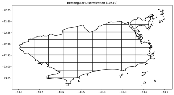
Figure 1: Space discretization of a region containing the city of Rio de Janeiro into $10\times 10=100$ rectangles, 76 of which have nonempty intersection with the region and are shown in the figure.

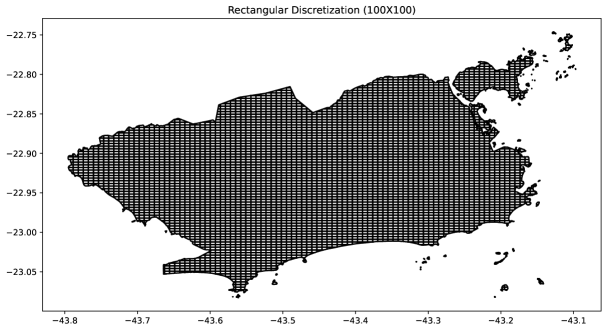
Figure 2: Space discretization of a region containing the city of Rio de Janeiro into $100\times 100=10000$ rectangles, 4916 of which have nonempty intersection with the region and are shown in the figure.

4.3 Equal Sized Hexagonal Space Discretization

Another simple space discretization in LASPATED partitions the region into equal sized hexagons, in such a way that adjacent hexagons share a common edge. (The Uber Python package H3 was used for the discretization.) Figure 3 shows a discretization of a region containing the city of Rio de Janeiro into hexagons using scale parameter equal to 7, and Figure 4 shows a discretization of the same region into hexagons using scale parameter equal to 8. Both discretizations were obtained with LASPATED.

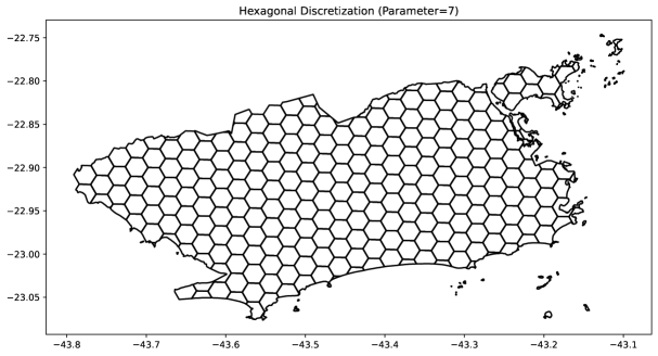
Figure 3: Space discretization of a region containing the city of Rio de Janeiro into hexagons using the Uber library H3 with scale parameter equal to $7$.

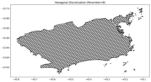
Figure 4: Space discretization of a region containing the city of Rio de Janeiro into hexagons using the Uber library H3 with scale parameter equal to $8$.

4.4 Customized Space Discretization

LASPATED also facilitates space discretization with customized subregions. For example, Figure 5 obtained with LASPATED displays a customized discretization of the city of Rio de Janeiro into $160$ administrative districts.

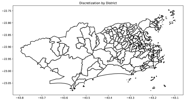
Figure 5: Space discretization of a region containing the city of Rio de Janeiro into 160 administrative districts.

4.5 Discretization using Voronoi diagrams

LASPATED also provides space discretization with Voronoi diagrams. Figure 6 obtained with LASPATED displays a discretization based on the Voronoi diagram given by the locations of ambulance stations in Rio de Janeiro. Each zone includes the set of points that are closest to a specific station.

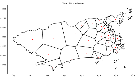
Figure 6: Discretization of a region containing the city of Rio de Janeiro into 34 subregions given by the Voronoi diagram of ambulance stations in Rio de Janeiro.

5 Additional Discretization Functionalities

Often different discretizations are used for different purposes. For example, different spatial attribute data such as population count and land use type may be provided using different space discretizations. Consider two discretizations $D_{1}$ and $D_{2}$. Let $\mathcal{I}_{1}$ be the index set of the subregions of discretization $D_{1}$, and let $\mathcal{I}_{2}$ be the index set of the subregions of discretization $D_{2}$. In this context, LASPATED provides the following functionalities:

• Given subregion indices $i_{1}\in\mathcal{I}_{1}$ and $i_{2}\in\mathcal{I}_{2}$, LASPATED computes the area $\mathcal{A}(i_{1},i_{2})$ of the intersection of subregions $i_{1}$ and $i_{2}$.

• Consider a given attribute, such as population count, and assume that the attribute value $P_{i_{1}}$ in each subregion $i_{1}\in\mathcal{I}_{1}$ of discretization $D_{1}$ is uniformly distributed with density $d_{i_{1}}=P_{i_{1}}/\mathcal{A}(i_{1})$, where $\mathcal{A}(i_{1})$ is the area of subregion $i_{1}$. We want to allocate this attribute value to the subregions of another discretization $D_{2}$. LASPATED computes the value of the attribute allocated to subregion $i_{2}\in\mathcal{I}_{2}$ of discretization $D_{2}$ as $\displaystyle\sum_{i_{1}\in\mathcal{I}_{1}}d_{i_{1}}\mathcal{A}(i_{1},i_{2})=\displaystyle\sum_{i_{1}\in\mathcal{I}_{1}}P_{i_{1}}\mathcal{A}(i_{1},i_{2})/\mathcal{A}(i_{1})$.

6 LASPATED Calibration Functions

LASPATED provides Matlab and C++ functions for the calibration of models as in Section 2.1 for given values of weights $W_{G}$ and $w_{i,j}$, by solving problem (10) using the projected gradient method with Armijo line search along a feasible direction or along the boundary.

LASPATED also provides Matlab and C++ cross validation functions for the selection of weights $W_{G}$ and $w_{i,j}$ and the computation of the corresponding optimal intensities $\lambda_{c.i.t}$ that solve problem (10) for the selected weights.

LASPATED also provides Matlab and C++ functions for the calibration of models with covariates as in Section 2.2. More precisely, it solves optimization problem (12) using projected gradient with Armijo line search along a feasible direction or along the boundary.

LASPATED includes the test examples for the calibration functions described in the next section.

7 Numerical Examples

7.1 Numerical Examples with Artificial Data without Covariates

In these examples, points arrive in $2$-dimensional space and over time according to a periodic non-homogeneous Poisson process. There is only one type of point, thus $|\mathcal{C}|=1$, and hence the type notation $c$ is omitted. The region under consideration is $\mathcal{S}=[0,10]^{2}$, as shown in Figure 7.

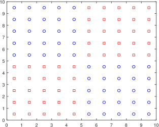
Figure 7: Example region $\mathcal{S}=[0,10]^{2}$. The intensity function $\lambda$ is different in the blue and red subregions, but the user does not know about these subregions. For estimation purposes, the user discretizes $\mathcal{S}$ into $10\times 10=100$ square zones.

The region $\mathcal{S}$ is partitioned into two subsets $\mathcal{S}=\mathcal{B}\cup\mathcal{R}$, with $\mathcal{B}=[0,5]\times(5,10]\cup(5,10]\times[0,5]$ and $\mathcal{R}=[0,5]\times[0,5]\cup(5,10]\times(5,10]$.

7.1.1 Example 1

In this example, the rate function $\lambda:\mathcal{S}\times[0,T]\mapsto\mathbb{R}_{+}$ is different on $\mathcal{B}$ and on $\mathcal{R}$, and is periodic with period $2$, as follows:

$$\lambda(s,t)\ \ =\ \ \left\{\begin{array}[]{lcl}0.1&\mbox{if}&s\in\mathcal{B}\mbox{ and }t\in(2k,2k+1]\mbox{ for some }k\in\mathbb{N},\\ 0.5&\mbox{if}&s\in\mathcal{B}\mbox{ and }t\in(2k-1,2k]\mbox{ for some }k\in\mathbb{N},\\ 0.5&\mbox{if}&s\in\mathcal{R}\mbox{ and }t\in(2k,2k+1]\mbox{ for some }k\in\mathbb{N},\\ 0.1&\mbox{if}&s\in\mathcal{R}\mbox{ and }t\in(2k-1,2k]\mbox{ for some }k\in\mathbb{N}.\end{array}\right.$$

This rate function is represented in Figure 8(a) (for time intervals that start at odd times) and Figure 8(b) (for time intervals that start at even times).

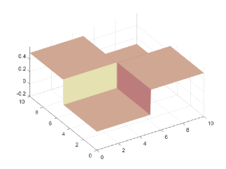
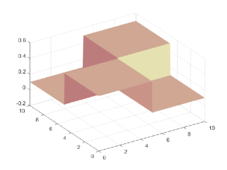
(a) Time intervals that start at odd times	(b) Time intervals that start at even times

Figure 8: Intensities as a function of location, for time intervals that start at odd times and even times.

The user knows the region $\mathcal{S}$ and that $|\mathcal{C}|=1$, but does not know about the subregions $\mathcal{B}$ and $\mathcal{R}$ that affect the intensity function $\lambda$, and does not know that $\lambda$ is periodic with period $2$. For estimation purposes, the user discretizes $\mathcal{S}$ into $100$ square zones of unit area each, as shown in Figure 7. Thus $\mathcal{I}=\mathcal{I}_{\mathcal{B}}\cup\mathcal{I}_{\mathcal{R}}$ indexes two types of zones, but this is not known by the user:

• $\mathcal{I}_{\mathcal{B}}$ indexes $50$ blue zones (with blue circles in their centers in Figure 7); there are $25$ blue zones in the bottom right and $25$ blue zones in the upper left of the region;

• $\mathcal{I}_{\mathcal{R}}$ indexes $50$ red zones (with red squares in their centers in Figure 7); there are $25$ red zones on the bottom left and $25$ red zones in the upper right of the region.

Also, for estimation purposes, the user discretizes time into $28$ time intervals of length $1$ each. Thus, the estimates are denoted with $\lambda_{i,t}$ for $i\in\mathcal{I}$ and $t\in\mathcal{T}\vcentcolon=\{1,\ldots,28\}$. Given arrival data $M_{i,t,n}$ for $i\in\mathcal{I}$, $t\in\mathcal{T}$, and $n=1,\ldots,N_{i,t}$, the regularized loss function in (2) is used to estimate $\lambda_{i,t}$. The penalty coefficients are $w_{i,j}=w>0$ when $i,j$ are neighboring zones, and $w_{i,j}=0$ otherwise, where $w$ will be varied as described later. Two zones are neighbors if their borders share an edge.

We consider two partitions $\mathcal{G}_{2}$ and $\mathcal{G}_{4}$ of time intervals $\mathcal{T}$ in (2). For partition $\mathcal{G}_{2}$, the time groups are $G_{0}=\{2k\,:\,k=1,\ldots,14\}$ and $G_{1}=\{2k+1\,:\,k=0,1,\ldots,13\}$. For partition $\mathcal{G}_{4}$, the time groups are $G_{0}=\{4k\,:\,k=1,\ldots,7\}$, $G_{1}=\{4k+1\,:\,k=0,1,\ldots,6\}$, $G_{2}=\{4k+2\,:\,k=0,1,\ldots,6\}$, and $G_{3}=\{4k+3\,:\,k=0,1,\ldots,6\}$. For both partitions, penalty coefficients $W_{G}=w$ for all groups $G$ (note that all groups have the same cardinality so that it seems reasonable to choose the same weights for different groups). Also, $\varepsilon=0.001$ in (11).

For any value of the penalty parameter $w$, let $\hat{\lambda}^{w}_{i,t}$ denote the estimator of $\lambda_{i,t}$ produced by (3). Note that when the penalty parameter $w=0$, then $\hat{\lambda}^{0}_{i,t}$ reduces to the empirical estimator of the intensities, which is the mean rate of arrivals in zone $i$ and time interval $t$. For a range of values of the penalty parameter $w$, we computed the estimates $\hat{\lambda}^{w}_{i,t}$, and Figure 9 shows the mean (over all zones $i$ and time intervals $t$) relative error given by

$$\frac{1}{|\mathcal{I}||\mathcal{T}|}\sum_{i\in\mathcal{I}}\sum_{t\in\mathcal{T}}\left|\frac{\lambda_{i,t}-\hat{\lambda}^{w}_{i,t}}{\lambda_{i,t}}\right|$$

as a function of penalty parameter $w$, for different values of $N_{i,t}$. Figure 9 shows the mean relative errors for the following four estimators: estimator with partition $\mathcal{G}_{4}$ of time intervals and with neighbor-based spatial regularization (legend “4 groups, neighbors” in the figure), estimator with partition $\mathcal{G}_{4}$ of time intervals and without spatial regularization (legend “4 groups, no neighbors” in the figure), estimator with partition $\mathcal{G}_{2}$ of time intervals and with neighbor-based spatial regularization (legend “2 groups, neighbors” in the figure), and estimator with partition $\mathcal{G}_{2}$ of time intervals and without spatial regularization (legend “2 groups, no neighbors” in the figure). Figure 9 presents results for three values of the sample size: $N_{i,t}=14$ periods observed, $N_{i,t}=140$ periods observed, and $N_{i,t}=700$ periods observed. Figure 9 also shows, for each sample size, the mean relative error obtained by choosing the penalty parameter $w$ by cross validation as follows: we partitioned the data into $5$ subsets. Then, for each of $5$ replications we used one of the data subsets (a different subset for each replication, with 20% of data used for training) to compute $\hat{\lambda}^{w}_{i,t}$ with partition $\mathcal{G}_{2}$ of time intervals and with neighbor-based spatial regularization for a range of values of $w$, and we used the remaining data to compute the mean relative error for each value of $w$. Then we determined the penalty parameter $w^{*}$ that minimizes the average mean relative error over the $5$ replications. Figure 9 shows the mean relative error for the resulting cross validation estimator with partition $\mathcal{G}_{2}$ of time intervals and with neighbor-based spatial regularization using the penalty parameter $w^{*}$. Note that the empirical estimator, with $w=0$, does not depend on the partition of time intervals and the neighbor structure, and therefore is given by all four estimators described above at $w=0$. Table 1 shows the minimum mean relative errors over different values of penalty parameter $w$, as well as the values of $w$ that attain the minimum, for each of the six estimators and for each of the three sample sizes considered in Figure 9.

Sample size $N_{i,t}$	Reg 1	Reg 2	Reg 3	Reg 4	CV	Emp
14	0.41/17	0.51/12	0.41/15	0.51/30	0.46/17	1.44/0
140	0.14/0.4	0.26/0.5	0.13/0.3	0.19/13	0.13/1	0.53/0
700	0.06/0.06	0.1/0.1	0.05/0.04	0.07/0.06	0.12/0.1	0.25/0

Table 1: For each sample size and for each estimator, each cell of the table gives two numbers separated by a slash (/): the first number is the minimum mean relative error over different values of penalty parameter $w$, and the second number is the value of $w$ that attain the minimum. The column headings denote the estimators as follows: Reg 1: estimator with partition $\mathcal{G}_{4}$ of time intervals and with neighbor-based spatial regularization; Reg 2: estimator with partition $\mathcal{G}_{4}$ of time intervals and without spatial regularization; Reg 3: estimator with partition $\mathcal{G}_{2}$ of time intervals and with neighbor-based spatial regularization; Reg 4: estimator with partition $\mathcal{G}_{2}$ of time intervals and without spatial regularization; CV: cross validation; Emp: empirical estimator.

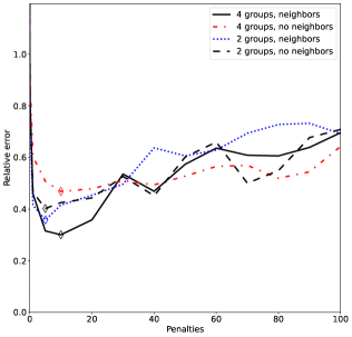
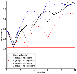
$N_{i,t}=14$ periods observed	$N_{i,t}=140$ periods observed

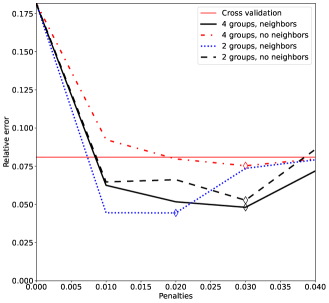
$N_{i,t}=700$ periods observed

Figure 9: Mean relative estimation errors $\frac{1}{|\mathcal{I}||\mathcal{T}|}\sum_{i\in\mathcal{I}}\sum_{t\in\mathcal{T}}\left|\frac{\lambda_{i,t}-\hat{\lambda}^{w}_{i,t}}{\lambda_{i,t}}\right|$ as a function of the penalty parameter $w$, for four sample sizes and six estimators (including the empirical estimator at $w=0$).

In Figure 9, note that the vertical and horizontal scales of the sub-figures are different. As expected, the estimation error is decreasing in the sample size $N_{i,t}$. Even when regularization is not based on the correct subregions and partition of time intervals, it can result in much better estimates than the empirical estimates (corresponding to $w=0$), as long as reasonable values are chosen for $w$. Furthermore, note that the mean relative errors shown in Figure 9, and the values of the penalty parameter $w$ with the smallest mean relative errors (shown with diamonds), were based on using the correct values $\lambda_{i,t}$ in the calculations, which are not known by the user. As explained before, we also used cross validation to determine good values of the penalty parameter $w$ (without knowing the correct values $\lambda_{i,t}$), resulting in mean relative errors for most experiments much smaller than the mean relative error of the empirical estimator.

The results indicate that the improvement of the estimates using regularization is more pronounced when the number of observations is small: for $N_{i,t}=14$, the estimation error decreases from about 120% (for the empirical estimator) to about 29% for the best regularized estimator, and for $N_{i,t}=140$, the estimation error decreases from about 40% to about 7%. Therefore, when a small amount of data are available, the regularized estimator results in a much smaller estimation error, even if the regularization is not based on the correct model structure, as long as relevant information is used for the regularization.

Figure 10 shows the true intensities $\lambda(s,t)$ and the estimates $\hat{\lambda}^{w^{*}}_{i,t}$ obtained with partition $\mathcal{G}_{2}$ of time intervals and with neighbor-based spatial regularization using the best penalty parameters $w^{*}$, for $s\in\mathcal{R}$, zone $1\in\mathcal{I}_{\mathcal{R}}$, $N_{i,t}=14$ (top left plot), for $s\in\mathcal{R}$, zone $1\in\mathcal{I}_{\mathcal{R}}$, $N_{i,t}=140$ (bottom left plot), for $s\in\mathcal{B}$, zone $6\in\mathcal{I}_{\mathcal{B}}$, $N_{i,t}=14$ (top right plot), and for $s\in\mathcal{B}$, zone $6\in\mathcal{I}_{\mathcal{B}}$, $N_{i,t}=140$ (bottom right plot). It can be seen that the regularized estimates are much closer to the true intensities than the empirical estimates.

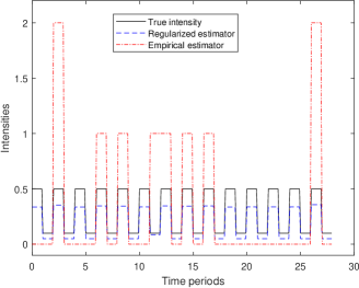
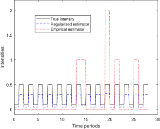
$N_{i,t}=14$, zone $1\in\mathcal{I}_{\mathcal{R}}$	$N_{i,t}=14$, zone $6\in\mathcal{I}_{\mathcal{B}}$
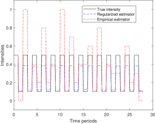
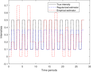
$N_{i,t}=140$, zone $1\in\mathcal{I}_{\mathcal{R}}$	$N_{i,t}=140$, zone $6\in\mathcal{I}_{\mathcal{B}}$

Figure 10: Comparison of true, empirical, and regularized estimates of the Poisson process intensities. True intensities as shown in Figure 8.

7.1.2 Example 2

In this example, we consider the same region $\mathcal{S}$ and the same subregions $\mathcal{B}$ and $\mathcal{R}$ as in Example 1. The intensity function $\lambda$ is also periodic, but not piecewise constant, as follows:

$$\lambda(x,y,t)\ \ =\ \ \left\{\begin{array}[]{lcl}x+y&\mbox{if}&(x,y)\in\mathcal{B}\mbox{ and }t\in(2k,2k+1]\mbox{ for some }k\in\mathbb{N},\\ 5(x+y)&\mbox{if}&(x,y)\in\mathcal{B}\mbox{ and }t\in(2k-1,2k]\mbox{ for some }k\in\mathbb{N},\\ 5(x+y)&\mbox{if}&(x,y)\in\mathcal{R}\mbox{ and }t\in(2k,2k+1]\mbox{ for some }k\in\mathbb{N},\\ x+y&\mbox{if}&(x,y)\in\mathcal{R}\mbox{ and }t\in(2k-1,2k]\mbox{ for some }k\in\mathbb{N}.\end{array}\right.$$

This rate function is represented in Figure 11(c) (for time intervals that start at odd times) and Figure 11(d) (for time intervals that start at even times).

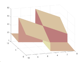
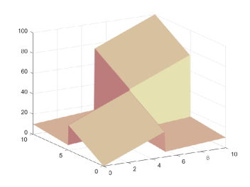
(c) Time intervals that start at odd times	(d) Time intervals that start at even times

Figure 11: Intensities as a function of location, for time intervals that start at odd times and even times.

As in Example 1, the user knows the region $\mathcal{S}$ and that $|\mathcal{C}|=1$, but does not know about the subregions $\mathcal{B}$ and $\mathcal{R}$ that affect the intensity function $\lambda$, and does not know that $\lambda$ is periodic with period $2$. For estimation purposes, the user discretizes $\mathcal{S}$ into $100$ square zones of unit area each. The user computes the estimators $\hat{\lambda}^{w}_{i,t}$ for each $i\in\mathcal{I}$ and each $t\in\mathcal{T}$, by solving optimization problem (10) using regularization with penalty parameter $w$ and $\varepsilon=0.001$. Each estimator $\hat{\lambda}^{w}_{i,t}$ now approximates the rate $\displaystyle\int_{R_{i}}\lambda(x,y,t)\mathop{}\!\mathrm{d}(x,y)$, where $R_{i}$ denotes the square of unit area for zone $i$. For example, for a zone $i$ with $R_{i}=(a_{i}-1,a_{i}]\times(b_{j}-1,b_{j}]$ and $\lambda(x,y,t)=x+y$ for $(x,y)\in R_{i}$, it holds that

$$\int_{R_{i}}\lambda(x,y,t)\mathop{}\!\mathrm{d}(x,y)\ \ =\ \ \int_{a_{i}-1}^{a_{i}}\int_{b_{j}-1}^{b_{j}}(x+y)\mathop{}\!\mathrm{d}x\mathop{}\!\mathrm{d}y\ \ =\ \ a_{i}+b_{j}-1\ \ =\ \ \lambda(x_{i},y_{i},t)\ \ =\ \ x_{i}+y_{i}$$

where $(x_{i},y_{i})=(a_{i}-0.5,b_{j}-0.5)$ is the centroid of zone $i$.

The mean relative error of estimator $\hat{\lambda}^{w}_{i,t}$ is now given by

$$\frac{1}{|\mathcal{I}||\mathcal{T}|}\sum_{i\in\mathcal{I}}\sum_{t\in\mathcal{T}}\frac{\left|\displaystyle\int_{R_{i}}\lambda(x,y,t)\mathop{}\!\mathrm{d}(x,y)-\hat{\lambda}^{w}_{i,t}\right|}{\displaystyle\int_{R_{i}}\lambda(x,y,t)\mathop{}\!\mathrm{d}(x,y)}\ \ =\ \ \frac{1}{|\mathcal{I}||\mathcal{T}|}\sum_{i\in\mathcal{I}}\sum_{t\in\mathcal{T}}\frac{\left|\lambda(x_{i},y_{i},t)-\hat{\lambda}^{w}_{i,t}\right|}{\lambda(x_{i},y_{i},t)}.$$

Parameter estimates $\hat{\lambda}^{w}_{i,t}$ were computed for a range of values of the penalty parameter $w$, for the same four estimators as in Example 1: estimator with partition $\mathcal{G}_{4}$ of time intervals and with neighbor-based spatial regularization (legend “4 groups, neighbors” in Figure 12), estimator with partition $\mathcal{G}_{4}$ of time intervals and without spatial regularization (legend “4 groups, no neighbors” in Figure 12), estimator with partition $\mathcal{G}_{2}$ of time intervals and with neighbor-based spatial regularization (legend “2 groups, neighbors” in Figure 12), and estimator with partition $\mathcal{G}_{2}$ of time intervals and without spatial regularization (legend “2 groups, no neighbors” in Figure 12). As before, four values were used for the sample size: $N_{i,t}=14$, $N_{i,t}=140$, $N_{i,t}=700$, and $N_{i,t}=7000$. Figure 12 shows the mean relative error for these four estimators, as well as the estimator with partition $\mathcal{G}_{2}$ of time intervals and with neighbor-based spatial regularization using the penalty parameter $w^{*}$ chosen with cross validation. As before, the empirical estimator corresponds to $w=0$. In this example, the mean relative errors are more sensitive regarding penalty parameter $w$ than in Example 1 with piecewise constant intensities. For small sample sizes, for some well-chosen penalties the regularized estimator mean relative error is smaller than the empirical mean relative error, whereas for large sample sizes, the empirical estimator is better than any other regularized estimator. This makes sense since regularization helps to compensate for the lack of data using appropriate, relevant information.

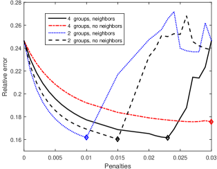
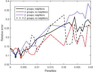
$N_{i,t}=14$ periods observed	$N_{i,t}=140$ periods observed
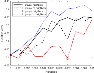
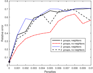
$N_{i,t}=700$ periods observed	$N_{i,t}=7000$ periods observed

Figure 12: Mean relative errors $\frac{1}{|\mathcal{I}||\mathcal{T}|}\displaystyle\sum_{t\in\mathcal{T}}\sum_{i\in\mathcal{I}}\frac{\left|\displaystyle\int_{R_{i}}\lambda(x,y,t)d(x,y)-{\hat{\lambda}}_{t,i}^{w}\right|}{\displaystyle\int_{R_{i}}\lambda(x,y,t)d(x,y)}$ as a function of the penalty parameter $w$. Intensities as in Figure 11.

7.2 Numerical Example with Artificial Data with Covariates

As in the previous examples, points arrive in $\mathcal{S}=[0,10]^{2}$ and over time according to a periodic nonhomogeneous Poisson process. Region $\mathcal{S}$ is partitioned into two subregions $\mathcal{S}=\mathcal{B}\cup\mathcal{R}$, with $\mathcal{B}=[0,5]\times(5,10]\cup(5,10]\times[0,5]$ and $\mathcal{R}=[0,5]\times[0,5]\cup(5,10]\times(5,10]$. There is only one type of point, thus $|\mathcal{C}|=1$, and hence the type notation $c$ is omitted. Each point $s\in\mathcal{S}$ has three attributes, denoted $x(s)\vcentcolon=(x_{1}(s),x_{2}(s),x_{3}(s))$. For example, $x_{1}(s)$ denotes the population density at location $s$, $x_{2}(s)=1$ if the land at location $s$ is used for commerce and $x_{2}(s)=0$ otherwise, and $x_{3}(s)=1$ if the land at location $s$ is used for manufacturing and $x_{3}(s)=0$ otherwise.

For the examples, $x(s)$ was generated as follows. Let $U^{b}_{j}$, $U^{r}_{j}$, $j=1,\ldots,20$, be independent random variables uniformly distributed on $(0,1)$. For $s\in\mathcal{B}$, let

$$x_{1}(s)\ \ =\ \ \sum_{j=1}^{10}\left(\frac{1}{2}\right)^{j}\left\{U^{b}_{2j-1}|\sin(2\pi js_{1}/10)|+U^{b}_{2j}|\sin(2\pi js_{2}/10)|\right\},$$

and for $s\in\mathcal{R}$, let

$$x_{1}(s)=\sum_{j=1}^{10}\left(\frac{1}{2}\right)^{j}\left\{(U^{r}_{2j-1}+1)|\sin(2\pi js_{1}/10)|+(U^{r}_{2j}+1)|\sin(2\pi js_{2}/10)|\right\}.$$

Let $x_{2}(s)=0.25$ and $x_{3}(s)=0.5$ for $s\in\mathcal{B}$, and $x_{2}(s)=0.5$ and $x_{3}(s)=0.25$ for $s\in\mathcal{R}$.

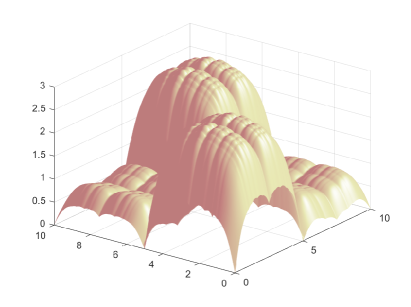
Figure 13: Graph of covariate function $x_{1}$.

We consider $2$ settings, one without a holiday effect, and one with a holiday effect. In both settings the rate function $\lambda$ is periodic with period $2$.

7.2.1 Example 3

In the setting without a holiday effect, the rate function $\lambda:\mathcal{S}\times[0,T]\mapsto\mathbb{R}_{+}$ is as follows:

$$\lambda(s,t)\ \ =\ \ \left\{\begin{array}[]{lcl}\beta(0)^{\top}x(s)&\mbox{if}&t\in(2k,2k+1]\mbox{ for some }k\in\mathbb{N},\\ \beta(1)^{\top}x(s)&\mbox{if}&t\in(2k-1,2k]\mbox{ for some }k\in\mathbb{N}\end{array}\right.$$

where

$$\begin{array}[]{ll}\beta_{1}(0)=0&\beta_{1}(1)=0.05,\\ \beta_{2}(0)=6&\beta_{2}(1)=18,\\ \beta_{3}(0)=3&\beta_{3}(1)=6.\end{array}$$

Thus, if $\mathcal{E}\vcentcolon=\cup_{k\in\mathbb{N}}(2k,2k+1]$ denotes the even-indexed time intervals and $\mathcal{O}\vcentcolon=\cup_{k\in\mathbb{N}}(2k-1,2k]$ denotes the odd-indexed time intervals, and $\mathcal{A}\subset\mathcal{S}$ and $\mathcal{D}\subset[0,\infty)$, then $\int_{\mathcal{D}}\int_{\mathcal{A}}\lambda(s,t)\mathop{}\!\mathrm{d}s\mathop{}\!\mathrm{d}t=\left|\mathcal{D}\cap\mathcal{E}\right|\beta(0)^{\top}\int_{\mathcal{A}}x(s)\mathop{}\!\mathrm{d}s+\left|\mathcal{D}\cap\mathcal{O}\right|\beta(1)^{\top}\int_{\mathcal{A}}x(s)\mathop{}\!\mathrm{d}s$, where $\left|\mathcal{D}\cap\mathcal{E}\right|\vcentcolon=\int_{\mathcal{D}\cap\mathcal{E}}\mathop{}\!\mathrm{d}t$ and $\left|\mathcal{D}\cap\mathcal{O}\right|\vcentcolon=\int_{\mathcal{D}\cap\mathcal{O}}\mathop{}\!\mathrm{d}t$.

7.2.2 Example 4

In the setting with a holiday effect, the rate function $\lambda:\{0,1\}\times\mathcal{S}\times[0,T]\mapsto\mathbb{R}_{+}$ is as follows:

$$\lambda(h,s,t)\ \ =\ \ \left\{\begin{array}[]{lcl}\beta(h,0)^{\top}x(s)&\mbox{if}&t\in(2k,2k+1]\mbox{ for some }k\in\mathbb{N},\\ \beta(h,1)^{\top}x(s)&\mbox{if}&t\in(2k-1,2k]\mbox{ for some }k\in\mathbb{N}\end{array}\right.$$

where $h=1$ if $t$ falls in a holiday, and $h=0$ otherwise, and

$$\begin{array}[]{llll}\beta_{1}(0,0)=0,&\beta_{1}(0,1)=0.05,&\beta_{1}(1,0)=0,&\beta_{1}(1,1)=0.1,\\ \beta_{2}(0,0)=6,&\beta_{2}(0,1)=18,&\beta_{2}(1,0)=12,&\beta_{2}(1,1)=36,\\ \beta_{3}(0,0)=3,&\beta_{3}(0,1)=6,&\beta_{3}(1,0)=6,&\beta_{3}(1,1)=12.\end{array}$$

We consider $2$ estimators for each of the $2$ settings: one estimator knows and uses aggregated covariate data, and the other estimator does not use covariate data. Below we describe the $2$ estimators in more detail.

7.2.3 Estimators that use the covariate data

The user knows the region $\mathcal{S}$ and that $|\mathcal{C}|=1$, but does not know that $\lambda$ is periodic with period $2$. In the setting with a holiday effect, the user knows that there is a holiday effect, but the user distinguishes $8$ different holidays and allows them to have different parameters. For estimation purposes, $\mathcal{S}$ is discretized into $100$ square zones of unit area each, as shown in Figure 7. Thus $\mathcal{I}=\mathcal{I}_{\mathcal{B}}\cup\mathcal{I}_{\mathcal{R}}$ indexes two types of zones, but this is not known by the estimator. For each zone $i\in\mathcal{I}$, the user observes only the aggregate value $y_{i,l}\vcentcolon=\displaystyle\int_{R_{i}}x_{l}(s)\mathop{}\!\mathrm{d}s$ of the covariate $x_{l}$ for the zone. For example, if a zone in $\mathcal{I}_{\mathcal{B}}$ is $[i-1,i)\times(j-1,j]$, then the aggregate value of the covariate $x_{1}$ for the zone is

$$\int_{i-1}^{i}\int_{j-1}^{j}x_{1}(s_{1},s_{2})\mathop{}\!\mathrm{d}s_{2}\mathop{}\!\mathrm{d}s_{1}$$

$$= \sum_{k=1}^{10}\left(\frac{1}{2}\right)^{k}\left\{U^{b}_{2k-1}\int_{i-1}^{i}|\sin(2\pi ks_{1}/10)|\mathop{}\!\mathrm{d}s_{1}+U^{b}_{2k}\int_{j-1}^{j}|\sin(2\pi ks_{2}/10)|\mathop{}\!\mathrm{d}s_{2}\right\}.$$

Therefore, we need to compute integrals of form $\displaystyle\int_{i-1}^{i}|\sin(2\pi ks_{1}/10)|\mathop{}\!\mathrm{d}s_{1}$.

Note that, for $0\leq s_{1}\leq 10$, it holds that $\sin(2\pi ks_{1}/10)\geq 0$ if

$$\frac{5}{k}\ell\ \ \leq\ \ s_{1}\ \ \leq\ \ \frac{5}{k}(\ell+1)\quad\mbox{and}\quad\ell\in\{0,1,\ldots,2k-2\}\mbox{ is even,}$$

and $\sin(2\pi ks_{1}/10)\leq 0$ if

$$\frac{5}{k}\ell\ \ \leq\ \ s_{1}\ \ \leq\ \ \frac{5}{k}(\ell+1)\quad\mbox{and}\quad\ell\in\{0,1,\ldots,2k\}\mbox{ is odd.}$$

Also note that

$$\frac{5}{k}\left\lceil\frac{k}{5}(i-1)\right\rceil\ \ \leq\ \ i\qquad\Longleftrightarrow\qquad\left\lceil\frac{k}{5}(i-1)\right\rceil\ \ \leq\ \ \frac{k}{5}i\qquad\Longleftrightarrow\qquad\left\lceil\frac{k}{5}(i-1)\right\rceil\ \ \leq\ \ \left\lfloor\frac{k}{5}i\right\rfloor.$$

Therefore, if $\frac{5}{k}\left\lceil\frac{k}{5}(i-1)\right\rceil\leq i$, then

$$\int_{i-1}^{i}|\sin(2\pi ks_{1}/10)|\mathop{}\!\mathrm{d}s_{1}$$

$$= \int_{i-1}^{\frac{5}{k}\left\lceil\frac{k}{5}(i-1)\right\rceil}|\sin(2\pi ks_{1}/10)|\mathop{}\!\mathrm{d}s_{1}+\sum_{\ell=\left\lceil\frac{k}{5}(i-1)\right\rceil}^{\left\lfloor\frac{k}{5}i\right\rfloor-1}\int_{\frac{5}{k}\ell}^{\frac{5}{k}(\ell+1)}|\sin(2\pi ks_{1}/10)|\mathop{}\!\mathrm{d}s_{1}+\int_{\frac{5}{k}\left\lfloor\frac{k}{5}i\right\rfloor}^{i}|\sin(2\pi ks_{1}/10)|\mathop{}\!\mathrm{d}s_{1}$$

$$= \frac{5}{\pi k}\left(-1\right)^{\left\lceil\frac{k}{5}(i-1)\right\rceil}\left[\cos\left(\pi\left\lceil\frac{k}{5}(i-1)\right\rceil\right)-\cos\left(\pi\frac{k}{5}(i-1)\right)\right]$$

$${}+\frac{10}{\pi k}\left(\left\lfloor\frac{k}{5}i\right\rfloor-\left\lceil\frac{k}{5}(i-1)\right\rceil\right)-\frac{5}{\pi k}\left(-1\right)^{\left\lfloor\frac{k}{5}i\right\rfloor}\left[\cos\left(\pi\frac{k}{5}i\right)-\cos\left(\pi\left\lfloor\frac{k}{5}i\right\rfloor\right)\right]$$

and if $\frac{5}{k}\left\lceil\frac{k}{5}(i-1)\right\rceil>i$, then

$$\int_{i-1}^{i}|\sin(2\pi ks_{1}/10)|\mathop{}\!\mathrm{d}s_{1}\ \ =\ \ \frac{5}{\pi k}\left(-1\right)^{\left\lfloor\frac{k}{5}i\right\rfloor}\left[\cos\left(\pi\frac{k}{5}(i-1)\right)-\cos\left(\pi\frac{k}{5}i\right)\right].$$

Also, $y_{i,2}\vcentcolon=\displaystyle\int_{R_{i}}x_{2}(s)\mathop{}\!\mathrm{d}s=0.25$, and $y_{i,3}\vcentcolon=\displaystyle\int_{R_{i}}x_{3}(s)\mathop{}\!\mathrm{d}s=0.5$ for $i\in\mathcal{I}_{\mathcal{B}}$, and $y_{i,2}=0.5$, and $y_{i,3}=0.25$ for $i\in\mathcal{I}_{\mathcal{R}}$.

As in the previous examples, time is discretized into $28$ time intervals of length $1$ each. The user’s model is the same as the model specified in Example 2.2, with $|\mathcal{C}|=1$, $|\mathcal{T}|=28$, $K_{1}=28$, and $|\mathcal{O}|=3$. Thus, in the setting without a holiday effect, the user’s intensity function $\hat{\lambda}:\mathcal{I}\times\mathcal{T}\mapsto\mathbb{R}_{+}$ given by

$$\hat{\lambda}(i,t)\ \ =\ \ \hat{\beta}(t)^{\top}y_{i}$$

estimates $\displaystyle\int_{R_{i}}\int_{(t-1,t]}\lambda(s,\tau)\mathop{}\!\mathrm{d}\tau\mathop{}\!\mathrm{d}s$, where $\hat{\beta}(t)=\big{(}\hat{\beta}_{1}(t),\hat{\beta}_{2}(t),\hat{\beta}_{3}(t)\big{)}$. Thus this estimated model has $28\times 3$ parameters. In the setting with a holiday effect, the user’s intensity function $\hat{\lambda}:\{0,1,\ldots,8\}\times\mathcal{I}\times\mathcal{T}\mapsto\mathbb{R}_{+}$ given by

$$\hat{\lambda}(h,i,t)\ \ =\ \ \hat{\beta}(h,t)^{\top}y_{i}$$

estimates $\displaystyle\int_{R_{i}}\int_{(t-1,t]}\lambda(h^{\prime},s,\tau)\mathop{}\!\mathrm{d}\tau\mathop{}\!\mathrm{d}s$, where $h^{\prime}=0$ if $h=0$ and $h^{\prime}=1$ if $h\in\{1,\ldots,8\}$, and $\hat{\beta}(h,t)=\big{(}\hat{\beta}_{1}(h,t),\hat{\beta}_{2}(h,t),\hat{\beta}_{3}(h,t)\big{)}$. Thus this estimated model has $9\times 28\times 3$ parameters.

7.2.4 Estimators that do not use the covariate values

The user knows the region $\mathcal{S}$ and that $|\mathcal{C}|=1$, but does not know about the subregions $\mathcal{B}$ and $\mathcal{R}$, does not know the covariate values $y_{i}$, and does not know that $\lambda$ is periodic with period $2$. In the setting with a holiday effect, the user knows that there is a holiday effect, but the user distinguishes $8$ different holidays and allows them to have different parameters.

The estimators are similar to those in Section 7.1. In the setting without a holiday effect, the user’s intensity function $\hat{\lambda}^{w}_{i,t}$, computed by solving (3) with penalty parameter $w$, estimates $\displaystyle\int_{R_{i}}\int_{(t-1,t]}\lambda(s,\tau)\mathop{}\!\mathrm{d}\tau\mathop{}\!\mathrm{d}s$. In the setting with a holiday effect, the user’s intensity function $\hat{\lambda}^{w}_{h,i,t}$, computed by solving (3) with penalty parameter $w$, estimates $\displaystyle\int_{R_{i}}\int_{(t-1,t]}\lambda(h^{\prime},s,\tau)\mathop{}\!\mathrm{d}\tau\mathop{}\!\mathrm{d}s$.

7.2.5 Numerical results

As in Section 7.1, we take penalities varying in the set $\{0.1,1,10,100,1000,10000\}$. We compare the mean relative error of the regularized estimator without covariates from Section 2.1 with penalty parameter $w^{*}$ and the estimator with covariates from Section 2.2 (without regularization).

The values of the best relative error $e_{*}$ (among all penalties for the regularized estimator from Section 2.1) are reported in Table 2 with column ”Holiday” indicating whether intensities are different on holidays or not. In this table, we consider three models without covariates: a model that does not use space regularization (No Cov 1 in the table), a model that uses space regularization with penalizing weights for neighbors of the same color (No Cov 2 in the table), and a model with space regularization with penalizing weights for all neighbors regardless of their color (No Cov 3 in the table). These experiments show that for this more complicated example, especially with holidays and limited data, estimators need to use a lot of data to be of good quality. The estimator based on covariates is much better and is of reasonable quality even if we do not have many observations (for 14 and 140 periods we only have one observation for each holiday and each time window of that holiday).

Available data	Holiday	Cov	No Cov 1	No Cov 2	No Cov 3	Emp
14 periods	No	7.0%	8.0%	6.0%	12.4%	25.1%
140 periods	No	4.0%	5.0%	8.0%	12.8%	16.0%
14 periods	Yes	17%	54.0%	53.3%	54.0%	54.0%
140 periods	Yes	14%	49%	48%	50%	56%

Table 2: Mean relative error $e_{*}$

7.3 Numerical experiment with real data

LASPATED was used with real data to calibrate arrival intensity functions for the process of medical emergencies reported to the Rio de Janeiro emergency medical service. The data included the date and time of the phone call, with the date ranging from 2016/01/01 to 2018/01/08, the location of the emergency, and the type of the emergency. The emergency type data included only a “priority level”: high, intermediate, and low-priority emergencies.

Different models of arrival intensity $\lambda_{c,i,t}$ as a function of emergency type $c$, location $i$, and time $t$, were calibrated. The calibrated models were periodic with a period of one week. The time of the week was discretized into time intervals of length $30$ minutes (thus the model had $T=7\times 48$ time intervals). Three different space discretizations were tested:

• A $10\times 10$ space discretization of a rectangle containing the city of Rio de Janeiro, shown in Figure 1 (76 of these rectangles have nonempty intersection with the city and are shown in the figure);

• A hexagonal discretization of the city of Rio de Janeiro (obtained with scale factor 7, with 297 hexagons intersecting Rio de Janeiro) shown in Figure 3;

• A discretization by administrative districts of the city of Rio de Janeiro (with 160 subregions), shown in Figure 5.

For each space discretization, the model without covariates described in Section 2.1 (called Model M1 in what follows), and the model with covariates described in Section 2.2 (called Model M2 in what follows), were calibrated with LASPATED. For the model with covariates, we used the following four covariates: (a) the population of the zone, (b) the land area of commercial activities and public facilities in the zone, (c) the land area of industrial activities in the zone, and (d) the non-populated land area (such as forests, beaches, and water) in the zone. For the calibration of Model M1, we set $w_{i,j}=w$ if zones $i$ and $j$ are neighbors, that is, if zones $i$ and $j$ share an edge or a vertex, and $w_{i,j}=0$ otherwise. The best value for $w$ was selected from $\{0,0.01,0.02,0.03,0.04,0.05\}$ using cross validation. We did not regularize by time groups. The optimization problems for calibration were solved using the projected gradient method with Armijo line search along a feasible direction.

Figure 14 shows the aggregated estimated intensities using the $10\times 10$ rectangular discretization. More specifically, the top left plot of Figure 14 shows $\sum_{c\in\mathcal{C}}\sum_{i\in\mathcal{I}}\hat{\lambda}_{c,i,t}$ as a function of $t$, the top right plot of Figure 14 shows $\sum_{i\in\mathcal{I}}\hat{\lambda}_{c_{2},i,t}$ where $c_{2}$ denotes the high-priority emergencies, the bottom left plot of Figure 14 shows $\sum_{i\in\mathcal{I}}\hat{\lambda}_{c_{1},i,t}$ where $c_{1}$ denotes the intermediate priority emergencies, and the bottom right plot of Figure 14 shows $\sum_{i\in\mathcal{I}}\hat{\lambda}_{c_{0},i,t}$ where $c_{0}$ denotes the low-priority emergencies. The intensity estimates shown in this figure are obtained with (i) the empirical mean number of calls for each call type, zone, and time interval, (ii) Model M1 with the $10\times 10$ rectangular space discretization, and (iv) Model M2 with the $10\times 10$ rectangular space discretization. In this example, all estimators give similar estimates of the aggregated intensities.

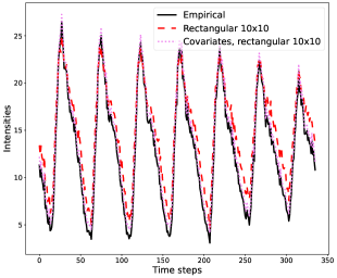
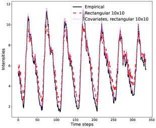
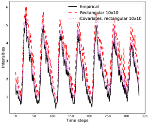
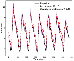
Figure 14: Aggregated estimates of the intensities for 3 estimators: (i) Empirical: the empirical intensities, (ii) Rectangular $10\times 10$: Model M1 with the $10\times 10$ rectangular space discretization, and (iii) Covariates, rectangular $10\times 10$: Model M2 with the $10\times 10$ rectangular space discretization. Top left: emergencies of all priorities, top right: high-priority emergencies, bottom left: intermediate priority emergencies, bottom right: low-priority emergencies.

Figure 15 shows the aggregated estimated intensities using discretization by district. The top left plot of Figure 15 shows $\sum_{c\in\mathcal{C}}\sum_{i\in\mathcal{I}}\hat{\lambda}_{c,i,t}$, the top right plot of Figure 15 shows $\sum_{i\in\mathcal{I}}\hat{\lambda}_{c_{2},i,t}$, the bottom left plot of Figure 15 shows $\sum_{i\in\mathcal{I}}\hat{\lambda}_{c_{1},i,t}$, and the bottom right plot of Figure 15 shows $\sum_{i\in\mathcal{I}}\hat{\lambda}_{c_{0},i,t}$. The intensity estimates shown in this figure are obtained with (i) the empirical number of calls for each call type, zone, and time interval, (ii) Model M1 with the space discretization by districts, and (iii) Model M2 with the space discretization by districts.

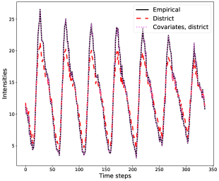
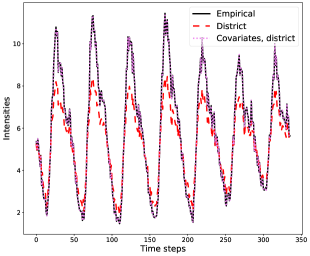
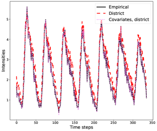
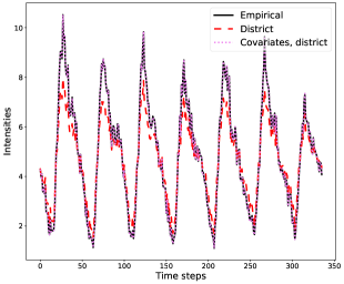
Figure 15: Aggregated estimates of the intensities for 3 estimators: (i) Empirical: the empirical intensities, (ii) District: Model M1 with the space discretization by districts, (iii) Covariates, district: Model M2 with the space discretization by districts. Top left: emergencies of all priorities, top right: high-priority emergencies, bottom left: intermediate priority emergencies, bottom right: low-priority emergencies.

Figure 16 shows the aggregated estimated intensities using hexagonal discretization with scale parameter 7. The top left plot of Figure 16 shows $\sum_{c\in\mathcal{C}}\sum_{i\in\mathcal{I}}\hat{\lambda}_{c,i,t}$, the top right plot of Figure 16 shows $\sum_{i\in\mathcal{I}}\hat{\lambda}_{c_{2},i,t}$, the bottom left plot of Figure 16 shows $\sum_{i\in\mathcal{I}}\hat{\lambda}_{c_{1},i,t}$, and the bottom right plot of Figure 16 shows $\sum_{i\in\mathcal{I}}\hat{\lambda}_{c_{0},i,t}$. The intensity estimates shown in this figure are obtained with (i) the empirical mean number of calls for each call type, zone, and time interval, (ii) Model M1 with hexagonal discretization with scale parameter 7, and (iii) Model M2 with hexagonal discretization with scale parameter 7.

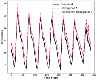
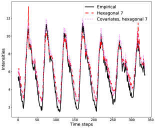
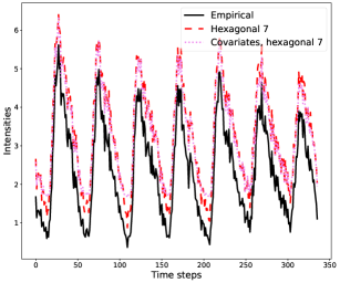
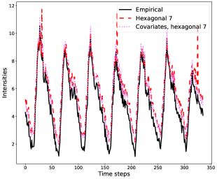
Figure 16: Aggregated estimates of the intensities for 3 estimators: (i) Empirical: the empirical intensities, (ii) Hexagonal 7: Model M1 with hexagonal discretization with scale parameter 7, and (iii) Covariates, hexagonal 7: Model M2 with hexagonal discretization with scale parameter 7. Top left: emergencies of all priorities, top right: high-priority emergencies, bottom left: intermediate priority emergencies, bottom right: low-priority emergencies.

Figure 17 shows heatmaps of the aggregated estimated intensities for emergencies of all priorities, for Model M1 and Model M2, using a $10\times 10$ rectangular space discretization. Figure 18 shows heatmaps of the aggregated estimated intensities for high-priority emergencies, for Model M1 and Model M2, using a $10\times 10$ rectangular space discretization. Figure 19 shows heatmaps of the aggregated estimated intensities for intermediate priority emergencies, for Model M1 and Model M2, using a $10\times 10$ rectangular space discretization. Finally, Figure 20 shows heatmaps of the aggregated estimated intensities for low-priority emergencies, for Model M1 and Model M2, using a $10\times 10$ rectangular space discretization.

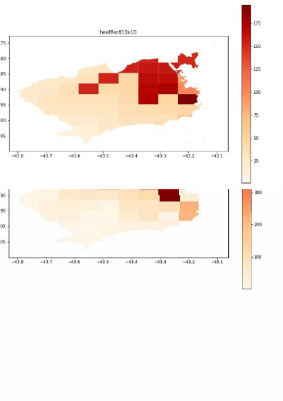
Figure 17: Heatmap of the aggregated estimated intensities for emergencies of all priorities for 2 estimators: Model M1 with a $10\times 10$ rectangular space discretization (top heatmap), and Model M2 with a $10\times 10$ rectangular space discretization (bottom heatmap).

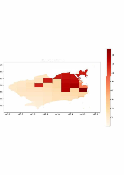
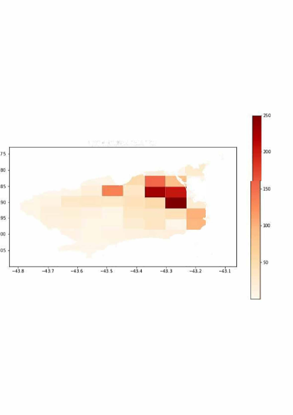
Figure 18: Heatmap of the aggregated estimated intensities for high-priority emergencies for 2 estimators: Model M1 with a $10\times 10$ rectangular space discretization (top heatmap), and Model M2 with a $10\times 10$ rectangular space discretization (bottom heatmap).

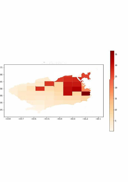
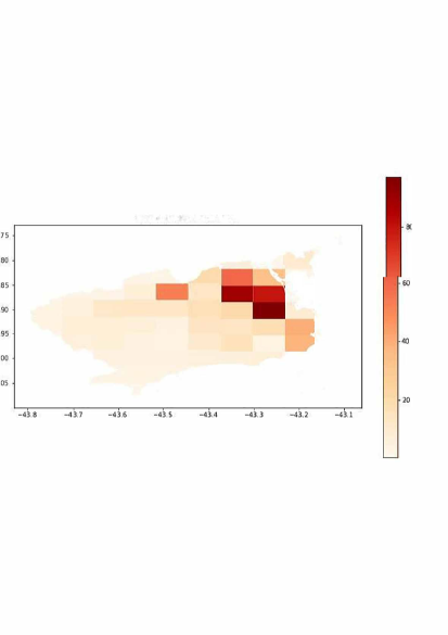
Figure 19: Heatmap of the aggregated estimated intensities for intermediate priority emergencies for 2 estimators: Model M1 with a $10\times 10$ rectangular space discretization (top heatmap), and Model M2 with a $10\times 10$ rectangular space discretization (bottom heatmap).

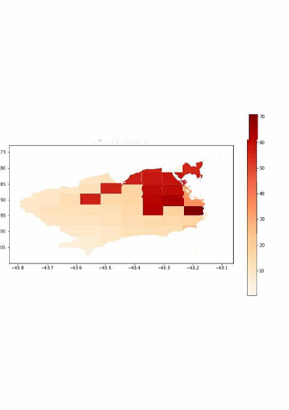
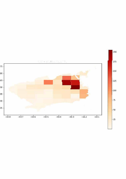
Figure 20: Heatmap of the aggregated estimated intensities for low-priority emergencies for 2 estimators: Model M1 with a $10\times 10$ rectangular space discretization (top heatmap), and Model M2 with a $10\times 10$ rectangular space discretization (bottom heatmap).

8 Conclusion

We described new models for stochastic spatio-temporal data and a software called LASPATED for discretization of space and time and for the calibration of such models. The library is public and external contributions to extend it are welcome.

As a future work, we plan to (i) design discretizations methods that adapt to the available data, (ii) develop calibration methods for combinations of non-parametric (low bias, high variance) models with parametric (high bias, low variance) models that use covariate data, (iii) develop methods to deal with missing data (for instance missing emergency location data), and (iv) include the corresponding tools into LASPATED.

References

- [1] V. Guigues, A. Kleywegt, and V.H. Nascimento. Operation of an ambulance fleet under uncertainty. arXiv, 2022.
- [2] A.N. Iusem. On the convergence properties of the projected gradient method for convex optimization. Computational and Applied Mathematics, 22(1):37–52, 2003.
- [3] G. Amorim Andre M. Krauss V.H. Nascimento V. Guigues, A. Kleywegt. LASPATED: a Library for the Analysis of SPAtio-TEmporal Discrete data, user manual. arXiv, 2023.