FTLE for Flow Ensembles by Optimal Domain Displacement

Abstract

FTLE (Finite Time Lyapunov Exponent) computation is one of the standard approaches to Lagrangian flow analysis. The main features of interest in FTLE fields are ridges that represent hyperbolic Lagrangian Coherent Structures. FTLE ridges tend to become sharp and crisp with increasing integration time, where the sharpness of the ridges is an indicator of the strength of separation. The additional consideration of uncertainty in flows leads to more blurred ridges in the FTLE fields. There are multiple causes for such blurred ridges: either the locations of the ridges are uncertain, or the strength of the ridges is uncertain, or there is low uncertainty but weak separation. Existing approaches for uncertain FTLE computation are unable to distinguish these different sources of uncertainty in the ridges.

We introduce a new approach to define and visualize FTLE fields for flow ensembles. Before computing and comparing FTLE fields for the ensemble members, we compute optimal displacements of the domains to mutually align the ridges of the ensemble members as much as possible. We do so in a way that an explicit geometry extraction and alignment of the ridges is not necessary. The additional consideration of these displacements allows for a visual distinction between uncertainty in ridge location, ridge sharpness, and separation strength. We apply the approach to several synthetic and real ensemble data sets.

D-FTLE optimal domain displaced flow maps of wind flow above the Indian Sea. Uncertainty is depicted with ellipses.

1 Introduction

FTLE (Finite Time Lyapunov Exponent) is probably the most popular approach to computing Lagrangian Coherent Structures (LCS) in time-dependent (unsteady) flows. FTLE is particularly tailored towards detecting hyperbolic LCS: regions of similar hyperbolic Lagrangian flow behavior are separated by ridge structures in the FTLE field. For increasing integration times, the increase in hyperbolic separation tends to lead to thin, crisp and sharp FTLE ridges. While the ridges are the main objective in analyzing FTLE fields, their numerical extraction is challenging in various aspects like accuracy, robustness and computational cost. For this reason, FTLE computation is still an active area of research.

In recent years, FTLE computation in the presence of uncertainty has moved into the focus of research. Several approaches exist for incorporating uncertainty into the analysis of FTLE fields. Although their basic concepts are diverse, existing approaches share one common behavior: under uncertainty, FTLE ridges tend to become more blurry, unsharp, and weak. We show that such blurry ridges in uncertain FTLE fields can have several reasons: either they are due to the presence of only a weak separation, or they are the result of some uncertainty about the ridges. In the latter case, two different kinds of uncertainty are possible: strength or location of the FTLE ridges. There may be a high uncertainty of the ridge location – we do not know where exactly the ridge is located – while the strength of the ridge is certain. Conversely, there may be no uncertainty about the exact location of the ridge, but the strength is uncertain.

We show that existing approaches for uncertain FTLE computation are unable to distinguish between the different kinds of the uncertainty about ridges as they produce a similar visual output: blurred ridges. We argue that FTLE ridges are the main objective of FTLE analysis and that a better understanding of the kind of uncertainty of FTLE ridges is necessary for an in-depth uncertain FTLE analysis.

In this paper, we present an approach to computing uncertain FTLE. Our approach works under the assumption that the input is an ensemble of velocity fields and enables distinguishing different kinds of uncertainty of the ridges. The main idea is to first find an optimal domain alignment of the flow maps, before FTLE is computed and compared for different ensemble members.

The input of our approach is an ensemble of $n$ velocity fields ${{\mathbf{v}}}_{1}({{\mathbf{x}}},t),\dots,{{\mathbf{v}}}_{n}({{\mathbf{x}}},t)$. We assume that ${{\mathbf{v}}}_{1},\dots,{{\mathbf{v}}}_{n}$ describe the same flow phenomenon with slightly different parameters. In particular, we assume that the LCS of ${{\mathbf{v}}}_{1},\dots,{{\mathbf{v}}}_{n}$ are similar and related to each other: for an FTLE ridge in ${{\mathbf{v}}}_{i}$, we can expect a similar FTLE ridge in ${{\mathbf{v}}}_{j}$ that is moved, continuously deformed, sharpened or weakened from the one in ${{\mathbf{v}}}_{i}$. This assumption is reasonable due to the nature of flow ensembles: they are typically produced by observing/simulating the same phenomenon under slightly different observation/simulation parameters. Our approach consists in computing small displacements of the domains of ${{\mathbf{v}}}_{1},\dots,{{\mathbf{v}}}_{n}$. We find a map from domain points to domain points, which leads to displacements (or “deformations”) of corresponding flow maps such that their FTLE ridges become aligned as much as possible. Based on this, we apply a visual analysis of the uncertain FTLE and the local displacement. This provides a tool for distinguishing the sources of FTLE uncertainty mentioned above.

2 Related Work

Before reviewing related work, we summarize different ways of representing uncertainty in flows. This is necessary to give a classification of existing work. There are two common ways to represent uncertainty: either by having an ensemble ${{\mathbf{v}}}_{1},...,{{\mathbf{v}}}_{n}$ of flows, or by having a velocity field ${{\mathbf{v}}}({{\mathbf{x}}},t)$ and a positive semidefinite matrix ${{\mathbf{D}}}({{\mathbf{x}}},t)$ describing the local diffusion of the flow. With ${{\mathbf{v}}}$ and ${{\mathbf{D}}}$ given, Monte Carlo integration techniques can be defined that assume an underlying Wiener process: the result of a stochastic integration step is independent of the steps in the past. While some existing approaches use estimations of ${{\mathbf{D}}}$ from the ensemble members ${{\mathbf{v}}}_{1},...,{{\mathbf{v}}}_{n}$, we argue that in general it is unclear if a valid estimation is possible. This is because a Monte Carlo integration may create trajectories that are not physically relevant, i.e., there is no underlying velocity field that fulfills the Navier Stokes equations. In fact, in general a barycentric combination of ${{\mathbf{v}}}_{1},...,{{\mathbf{v}}}_{n}$ does not fulfill the Navier Stokes equations, even if each ensemble member ${{\mathbf{v}}}_{i}$ does. We are not aware of reliable conditions under which ${{\mathbf{D}}}$ can be reliably estimated from ${{\mathbf{v}}}_{1},...,{{\mathbf{v}}}_{n}$. Because of this, our approach restricts to the trajectories of the ensemble members without having a Monte Carlo integration involved.

2.1 FTLE and FTLE ridges

One of the most prominent approaches to find LCS is the computation of ridge structures in scalar (FTLE) fields, as introduced by Haller [Hal01, HY00], see also [Hal15] for an introduction to LCS, their meaning for describing flow dynamics and their extraction via FTLE. FTLE ridges have been used for a variety of applications [Hal02, LCM^∗05, WPJ^∗08, SLP^∗09]. Shadden et al. [SLM05a] have shown that ridges of FTLE are approximate material structures, i.e., they converge to material structures for increasing integration times. This fact was used in [SW10] to extract topology structures. [LM10] and [SPFT12] introduce methods for tracking FTLE ridges by locally sampling the FTLE field and estimating the ridge direction and location. Due to the discrete sampling used, the accuracy is limited, especially for very sharp ridges. In [FH12] the minor eigenvector of the Cauchy-Green tensor is integrated to track ridge structures. This approach is, however, prone to accumulating integration errors. Also in the visualization community, different approaches have been proposed to increase performance, accuracy and usefulness of FTLE as a visualization tool [GLT^∗07, GGTH07, SP07a, SP07b, SRP09, GOPT11, PPF^∗11]. Haller and Sapsis [HS11] additionally explore the smallest FTLE values.

While most approaches mentioned above restrict themselves to ridge curves in 2D flows, there are a few approaches that extract ridge surfaces in 3D flows for moderate integration times. Schindler et al. [SPFT12] show both, standard height ridge extraction and C-ridge tracking to get 3D surfaces. [SFB^∗12] show C-ridge surfaces for an analysis of revolving doors. Sadlo and Peikert [SP07a] present FTLE ridge surfaces where with focus on an adaptive grid generation. Üffinger et al. [ÜSE13] present streak surfaces as approximations to FTLE ridges. Depending on the accuracy of the seed structures (obtained by extremely high sampling), streak surfaces and FTLE ridges show strong agreement. [BT13] propose an adaptive smooth reconstruction of the flow map field from the sample points based on Sibson’s interpolant on which the ridge extraction is more stable than on the original sampling.

2.2 Local uncertainty in vector fields

Local approaches describe uncertainty as a feature that can be evaluated at a point inside the vector field domain without considering the field’s “long-term” integral behavior. Sanderson et al. [SJK04] describe patterns of uncertainty using a reaction-diffusion model, while Botchen et al. [BWE05] introduce a texture-based visualization technique, that represents local reliabilities by cross advection and error diffusion. The same authors used additional color schemes to emphasize uncertainty [BWE06]. Another approach by Zuk et al. [ZDG^∗08] uses bidirectional vector fields to illustrate the impact of uncertainty.

2.3 Uncertainty for stream lines and path lines

There exist several approaches for capturing global behavior of stream lines and path lines for ensembles of vector fields in the literature. The perhaps simplest and most direct approach are spaghetti plots which provide straightforward overviews but tend to produce visual clutter [FBW16]. Mirzargar et al. [MWK14] introduce curve box-plots for the visualization of curve-like features based on the concept of statistical data depth. Otto et al. [OGHT10, OGT11] present a topological approach that is based on the integration of vector PDF. A related method by He et al. [HCLS16] for integrating uncertain stream lines is based on a Bayesian model. Hollister and Pang [HP20] present a method to measure uncertainty and to visualize member stream lines from an ensemble of vector fields by incorporating velocity probability density as a feature along each member stream line. Ferstl et al. [FBW16] derive stream line variability plots by computing a probabilistic mixture model for the stream line distribution, from which confidence regions can be derived in which the stream lines are most likely to reside. For a detailed overview of visualization on ensemble data we refer to the recent survey by Wang et al. [WHLS18].

2.4 FTLE and uncertainty

Schneider et al. [SFRS12] introduce Finite Time Variance Analysis (FTVA), a variance based FTLE-like method. The main idea is to integrate several runs of particles along with their spatial neighbors, and apply PCA to the resulting point sets. Guo et al. [GHP^∗16] introduce several approaches for uncertain FTLE computation: D-FTLE computes the FTLE field for every run and then considers the mean and the variance of the resulting scalar fields. FTLE-D computes the flow map gradient for each run and then considers its average for FTLE computation. Guo et al. [GHS^∗19] introduce an approach for particle tracing in uncertain flows. Haller et al. [HKK20] develop a mathematical theory for weakly diffusive tracers to predict transport barriers and enhancers solely from the flow velocity, without reliance on diffusive or stochastic simulations. A fast implementation of it is presented by Rapp et al. [RD20].

3 Notation and Problem Setting

Given is an ensemble of $n$ time-dependent $q$-dimensional ($q=2,3$) flow data sets over the same spatial domain $D\subset{{\mathbb{R}}}^{q}$ and temporal domain $T=[t_{s},t_{e}]$

$${{\mathbf{v}}}_{i}:D\times T \to {{\mathbb{R}}}^{q}$$

$$({{\mathbf{x}}},t) \to {{\mathbf{v}}}_{i}({{\mathbf{x}}},t)\qquad\text{for}~{}i=1,\dots,n\,.$$

We consider the flow maps

$$\phi_{i}:D\times T\times T \to D$$

$$({{\mathbf{x}}},t,\tau) \to \phi_{i}({{\mathbf{x}}},t,\tau)~{},$$

which describe the location of a massless particle that is seeded at $({{\mathbf{x}}},t)$ and integrated in ${{\mathbf{v}}}_{i}$ over a time interval $\tau$ such that $t+\tau\in T$. As a consequence, $\phi_{i}$ must satisfy

$$\frac{\partial\phi_{i}({{\mathbf{x}}},t,\tau)}{\partial\tau}={{\mathbf{v}}}_{i}\left(\phi_{i}({{\mathbf{x}}},t,\tau),t+\tau\right)\quad\text{with}\quad\phi_{i}({{\mathbf{x}}},t,0)={{\mathbf{x}}}~{}$$

for all ${{\mathbf{x}}}\in D$, $t\in T$, $t+\tau\in T$. Note that we assume for simplicity that the integration of ${{\mathbf{v}}}_{i}$ does not leave the domain $D$.

Based on this, we consider the standard definition of FTLE as

$$\mbox{FTLE}_{i}({{\mathbf{x}}},t,\tau)=\frac{1}{|\tau|}\ln\sqrt{\lambda_{\max}\left((\nabla\phi_{i})^{T}\,\nabla\phi_{i}\right)}$$

for $i=1,\dots,n$, where $\nabla\phi_{i}=\nabla\phi_{i}({{\mathbf{x}}},t,\tau)$ is the spatial gradient of $\phi_{i}$ and $\lambda_{\max}$ denotes the largest eigenvalue of a matrix.

A common approach in the literature is creating more than $n$ flow maps by a probabilistic process like repeated Monte Carlo integration. Such approaches consider a local distribution of the velocity field and use the assumption that the Monte Carlo integration is a Wiener process, i.e., the probability distribution for each integration step is independent of the integration results from the past. For flow ensembles we do not make this assumption because only the presence of ensemble members does not allow to estimate a local distribution of a vector field under consideration of a Wiener process.

Within this setup, existing approaches for uncertain FTLE computation can be summarized as follows: provide a visual representation and analysis of the distribution of

$$\phi_{1},\dots,\phi_{n}\quad\text{or}\quad\nabla\phi_{1},\dots,\nabla\phi_{n}\quad\text{or}\quad\mbox{FTLE}_{1},\dots,\mbox{FTLE}_{n}~{},$$ (1)

where different assumptions on the distribution and different options for a visual representation exist.

4 An Introductory Example

To illustrate the issues with existing FTLE approaches, we construct three ensembles containing 50 members each. We define a family of steady template vector fields

$${{\mathbf{v}}}^{k,r}({{\mathbf{x}}})=k\;{{\mathbf{v}}}_{DG}({{\mathbf{x}}},r)$$

where ${{\mathbf{v}}}_{DG}$ is the double gyre field from [SLM05b] (see (13) in the 2D domain ${{\mathbf{x}}}\in[0,2]\times[0,1]$ with two parameters $k>0$ and $r$, where time $t=r$. For computing the flow map and FTLE of ${{\mathbf{v}}}^{k,r}({{\mathbf{x}}})$, we choose $\tau=1$. This way, ${{\mathbf{v}}}^{k,r}$ consists of an LCS that is represented by the FTLE ridge whose location depends on $r$. Further, the strength of separation (corresponding to the sharpness of FTLE ridges) is controlled by $k$: the larger $k$, the sharper the FTLE ridge.

We define three ensembles with 50 members each:

$$E_{1} : {{\mathbf{v}}}_{1}={{\mathbf{v}}}^{5,\,-0.4},\,\dots,\,{{\mathbf{v}}}_{25}={{\mathbf{v}}}^{5,\,0},\,\dots,\,{{\mathbf{v}}}_{50}={{\mathbf{v}}}^{5,\,0.4}$$

$$E_{2} : {{\mathbf{v}}}_{1}={{\mathbf{v}}}^{2,\,0},\,\dots,\,{{\mathbf{v}}}_{25}={{\mathbf{v}}}^{3,\,0},\,\dots,\,{{\mathbf{v}}}_{50}={{\mathbf{v}}}^{4,\,0}$$

$$E_{3} : {{\mathbf{v}}}_{1}={{\mathbf{v}}}^{2,\,0},\,\dots,\,{{\mathbf{v}}}_{25}={{\mathbf{v}}}^{2,\,0},\,\dots,\,{{\mathbf{v}}}_{50}={{\mathbf{v}}}^{2,\,0}.$$

This definition implies the following properties of uncertainty:

• In $E_{1}$ there is low uncertainty about the strength of the FTLE ridge: each ensemble member has an FTLE ridge of approximately the same strength. But there is high uncertainty about the location of the ridges: the ridges of the ensemble members are all in different locations.

• In $E_{2}$ there is high uncertainty about the strength of the FTLE ridge: the ensemble members have an FTLE ridges of different strength. But there is a low uncertainty about the location of the ridges: all ensemble members have the ridge at the same location.

• In $E_{3}$ there is low uncertainty about the strength of the FTLE ridge and low uncertainty about the location of the ridges. In fact, this ensemble does not have any uncertainty at all because all ensemble members are identical. However, the strength of separation is weaker than in $E_{1}$ and $E_{2}$.

The ensemble $E_{1}$ is illustrated in figure 1. In the left column we see the FTLE fields of the ensemble members, while the right column gives a collection of standard uncertain FTLE measures (from top to down: D-FTLE, variance of D-FTLE, FTVA. They show a common behavior: a rather blurry ridge near the line $x=1$. Due to the 50 ensembles with a slight difference in the ridge position, there is no possibility to detect the source of the blurred ridge in the D-FTLE image. The variance does not help as it could also indicate variance in ridge strength.

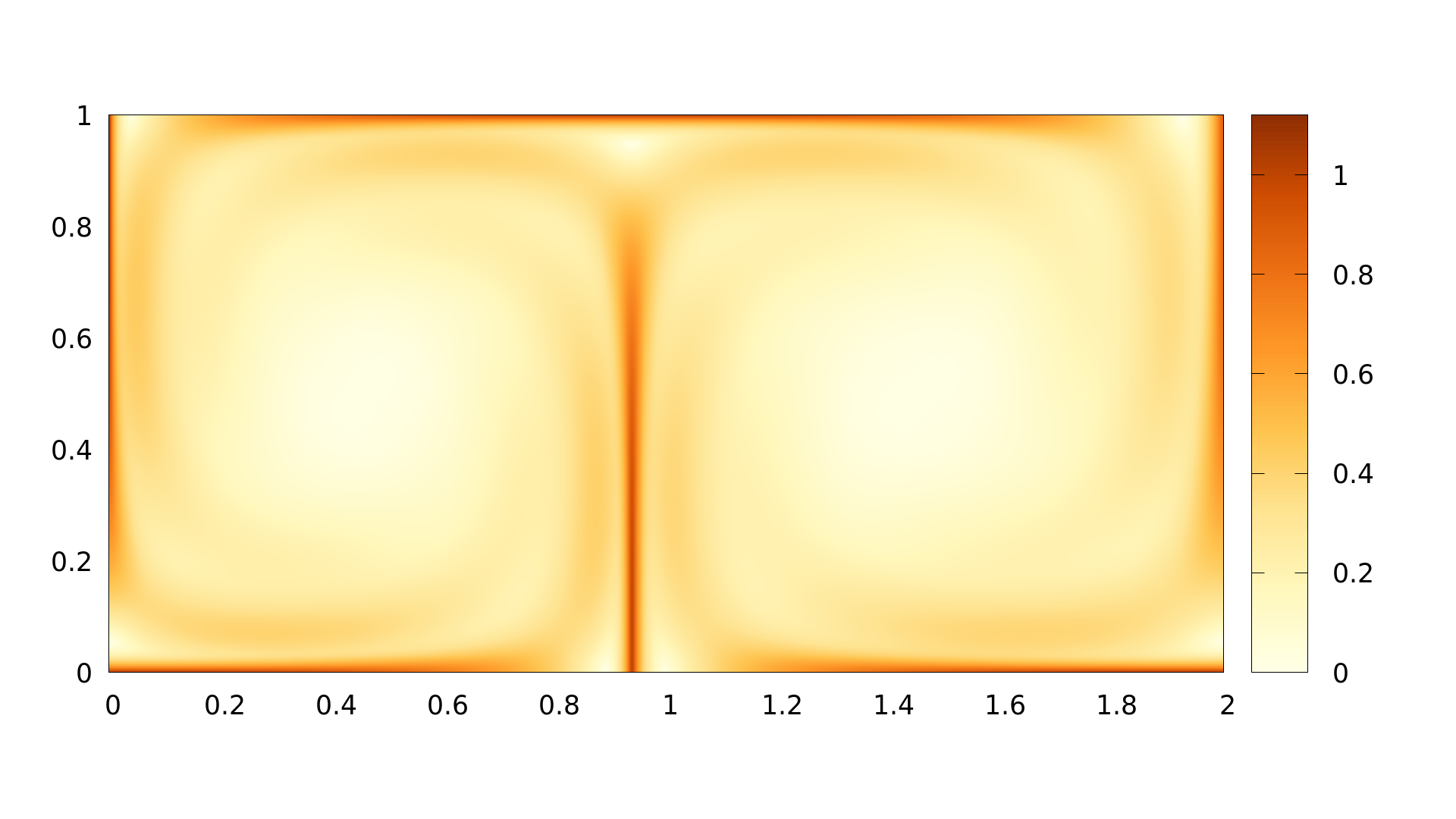
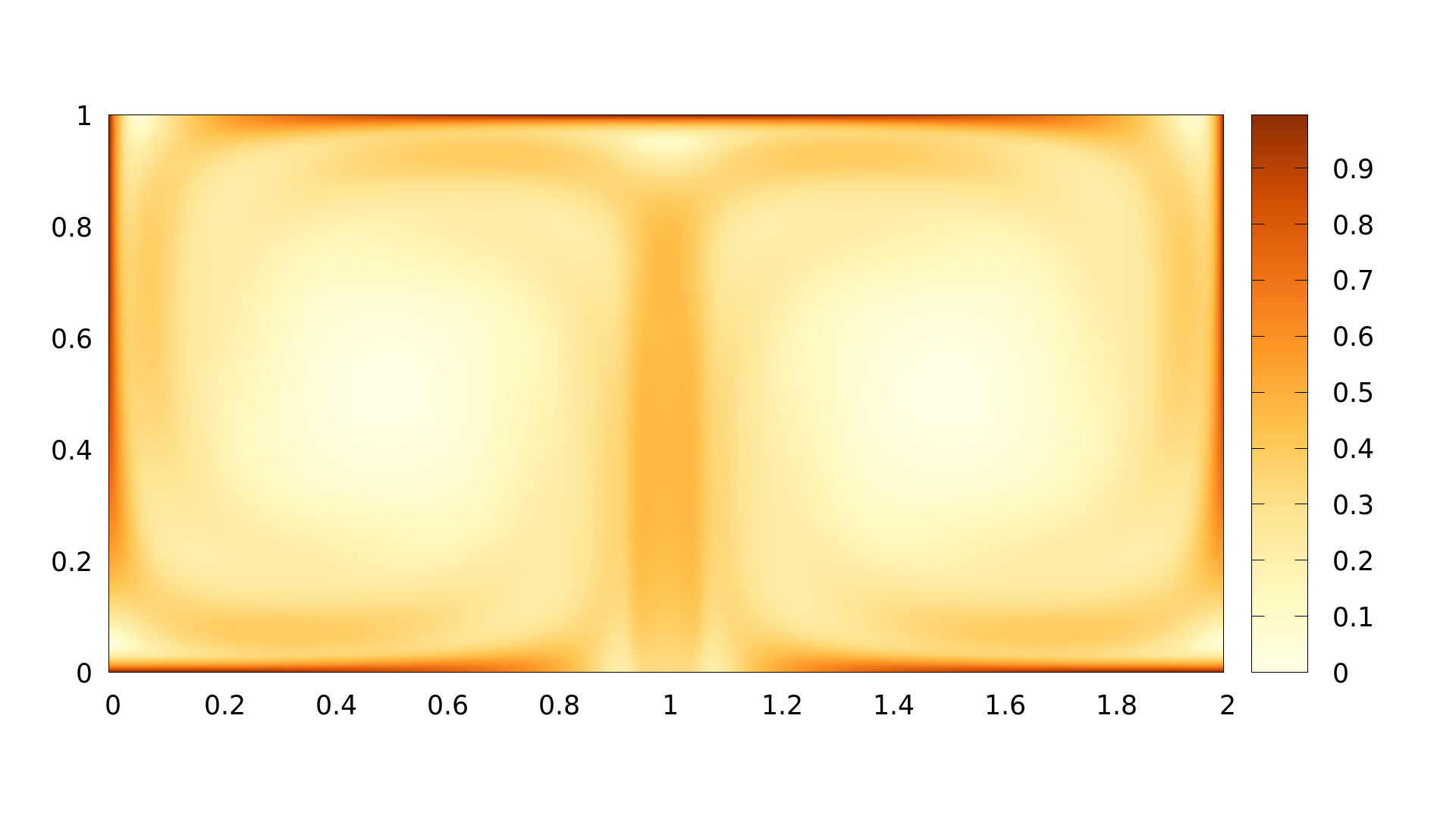
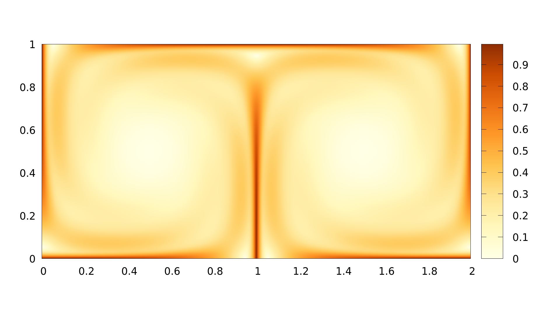
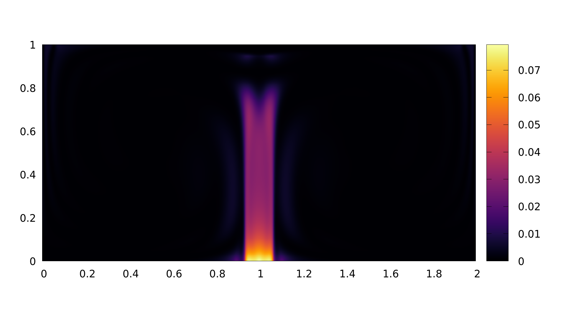
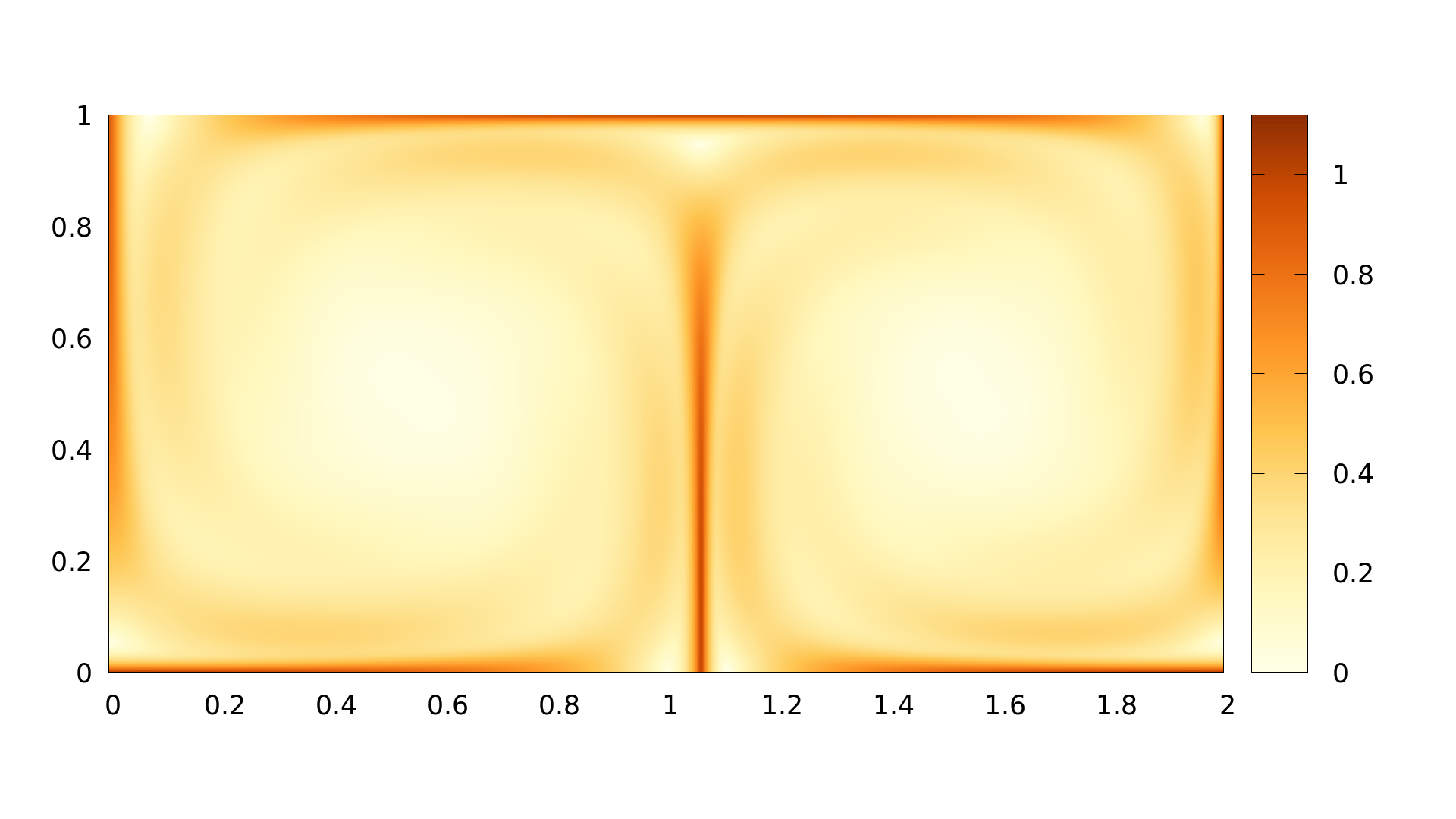
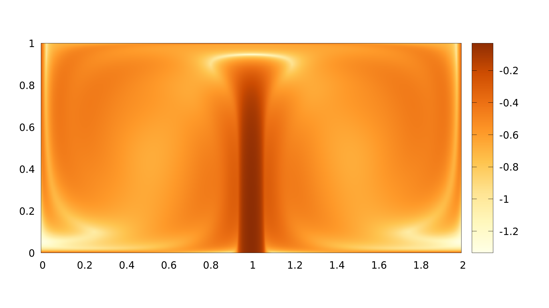
Figure 1: Ensemble $E_{1}$. Left column from top to bottom: FTLE of ensemble members $r=-0.4$, $r=0$, $r=0.4$. Right column from top to bottom: D-FTLE, variance of D-FTLE, FTVA of the ensemble.

Ensemble $E_{2}$ is illustrated figure 2. In the left column we see the FTLE fields of the ensemble members, the right column gives a collection of standard uncertain FTLE measures (from top to down: D-FTLE, variance of D-FTLE, FTVA. They also show a rather blurry ridge around the line $x=1$.

Finally, figure 3 gives an illustration of ensemble $E_{3}$: in the left column we see the FTLE fields of the ensemble members, while right column gives a collection of standard uncertain FTLE measures (from top to bottom: D-FTLE, variance of D-FTLE,s FTVA. They also show a rather blurry ridge around the line $x=1$. In fact, here we have identical ensemble members having a weak separation. The variance of D-FTLE is $0$.

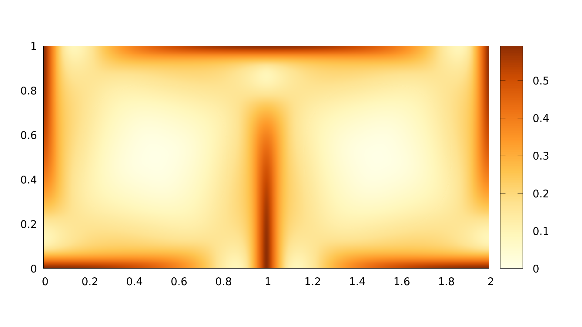
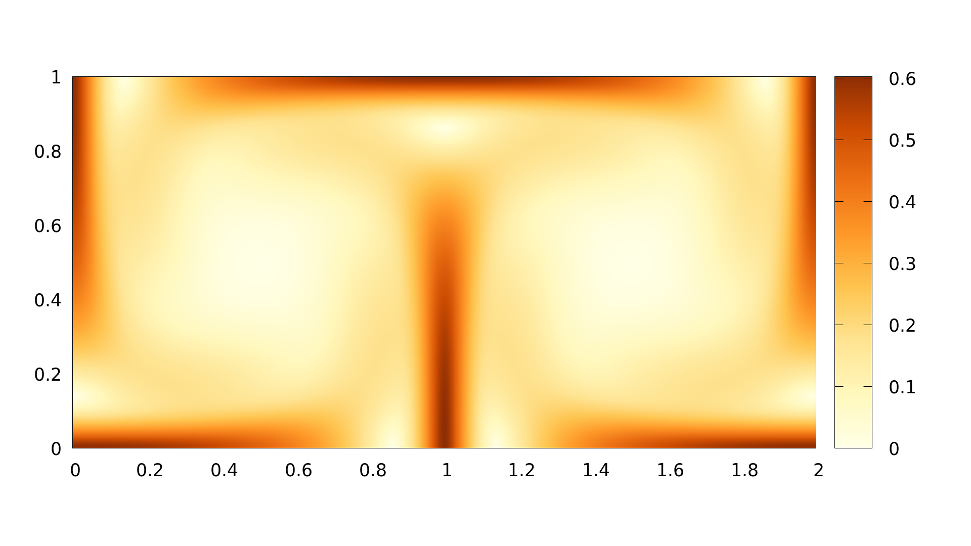
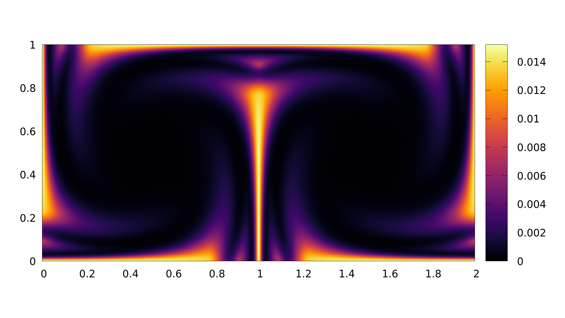
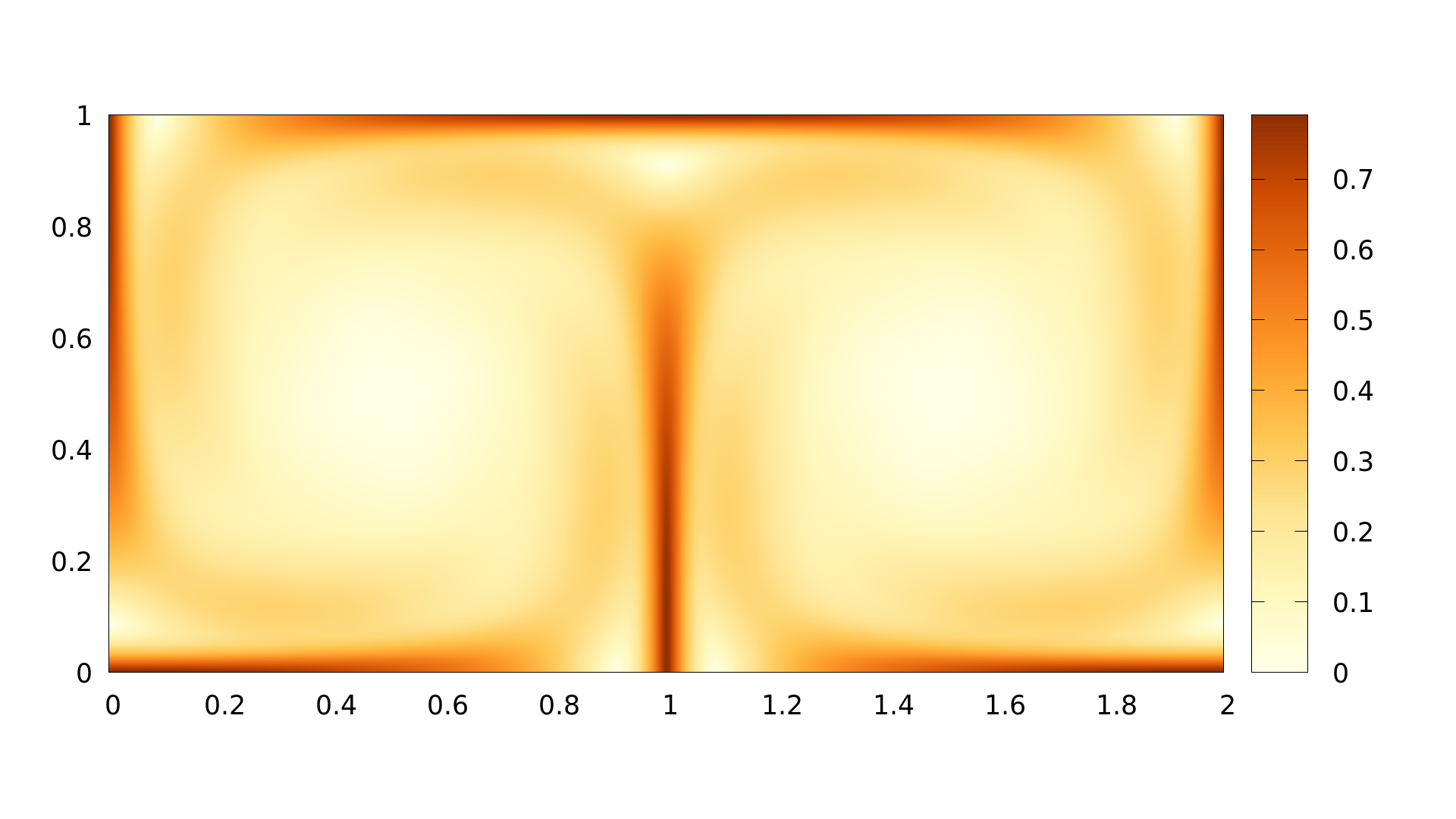
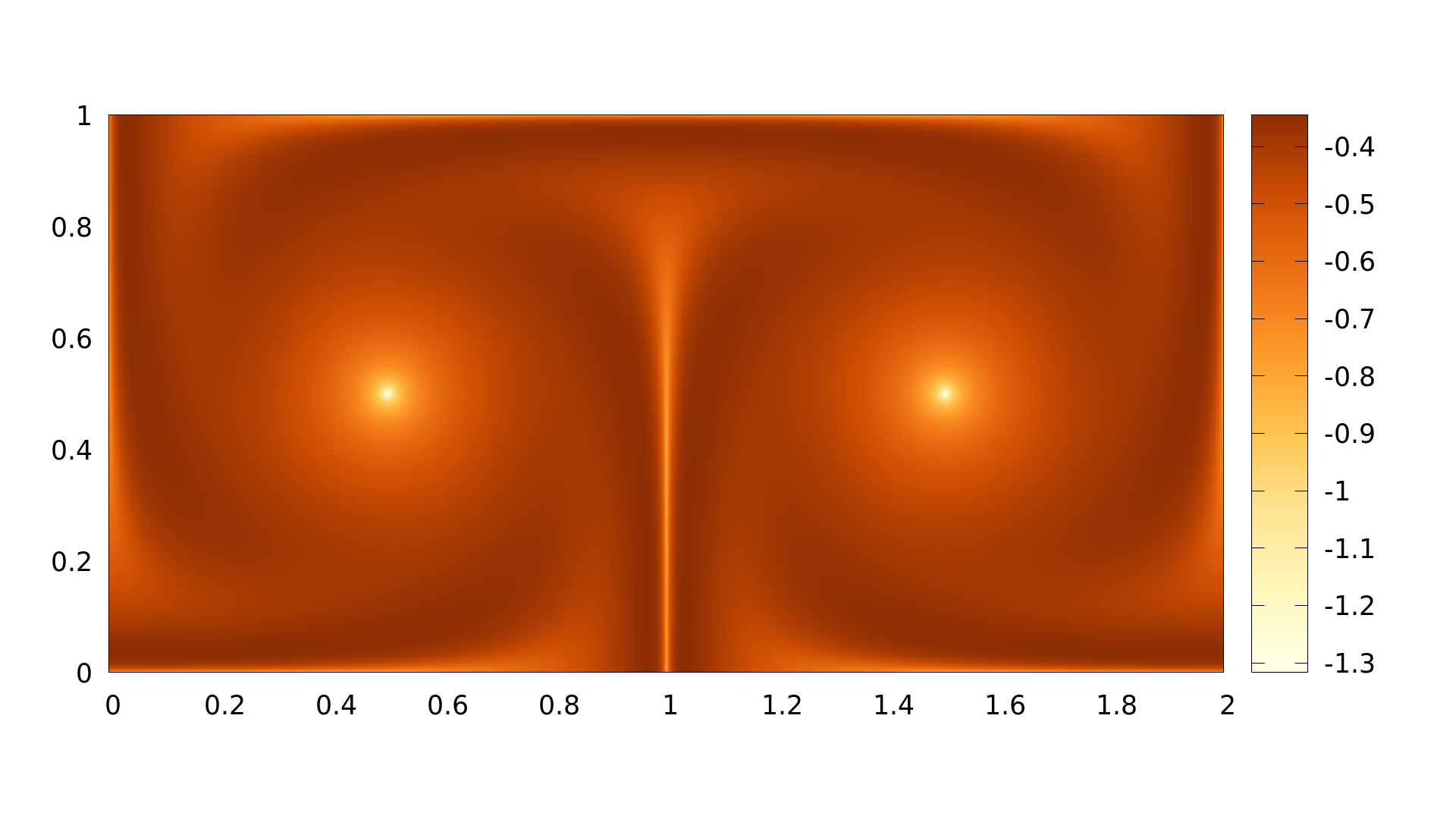
Figure 2: Ensemble $E_{2}$. Left row from top to bottom: FTLE of ensemble runs with $k=2$, $k=3$, $k=4$,.
Right row from top to bottom: D-FTLE, variance of D-FTLE, FTVA.

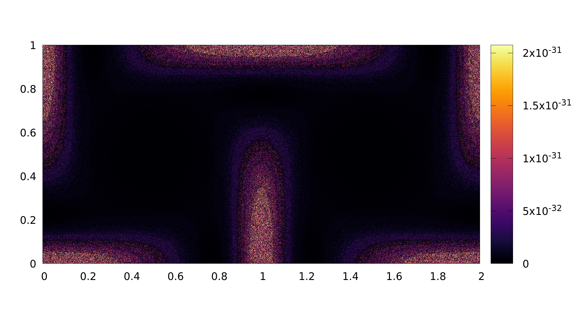
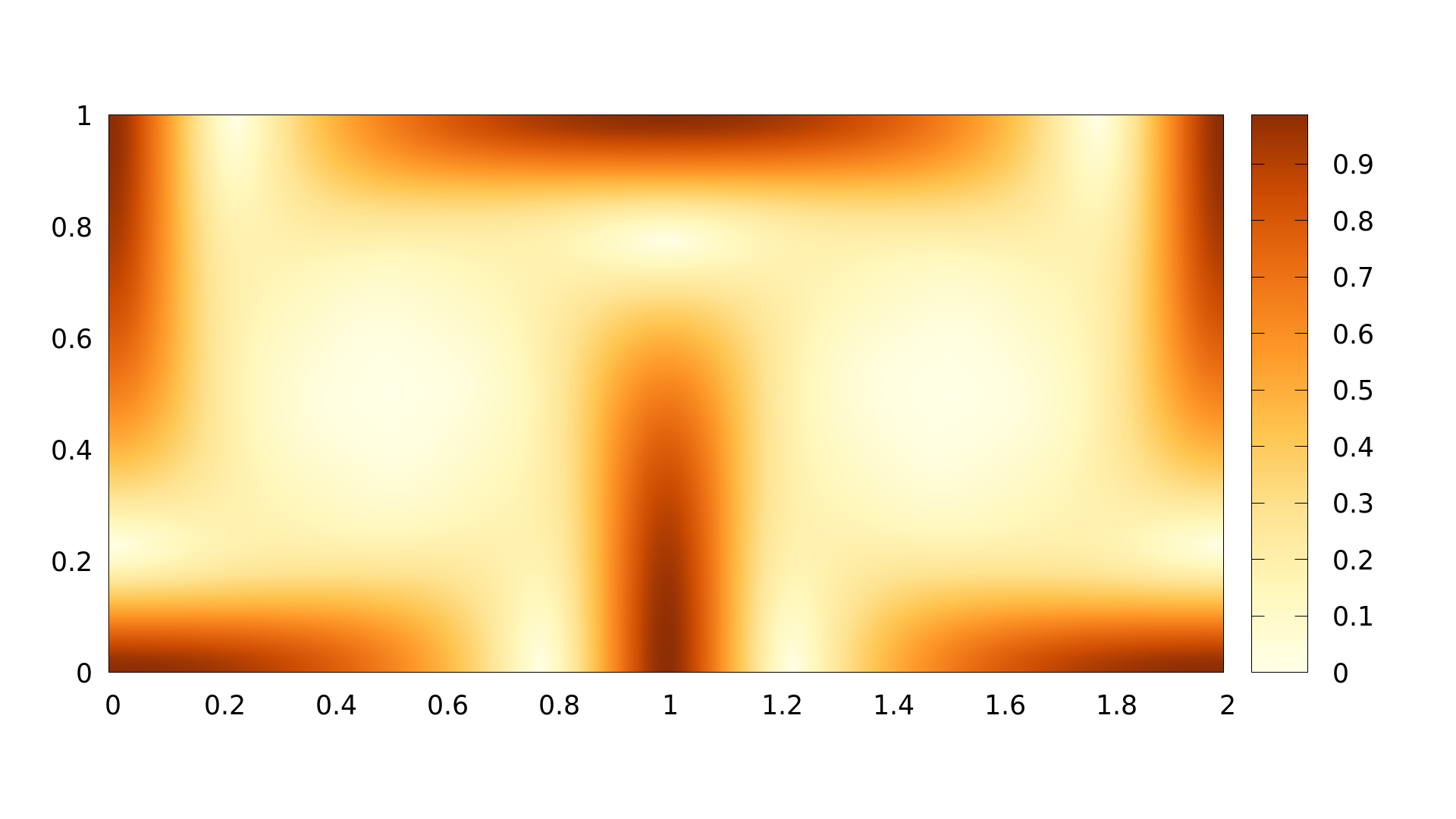
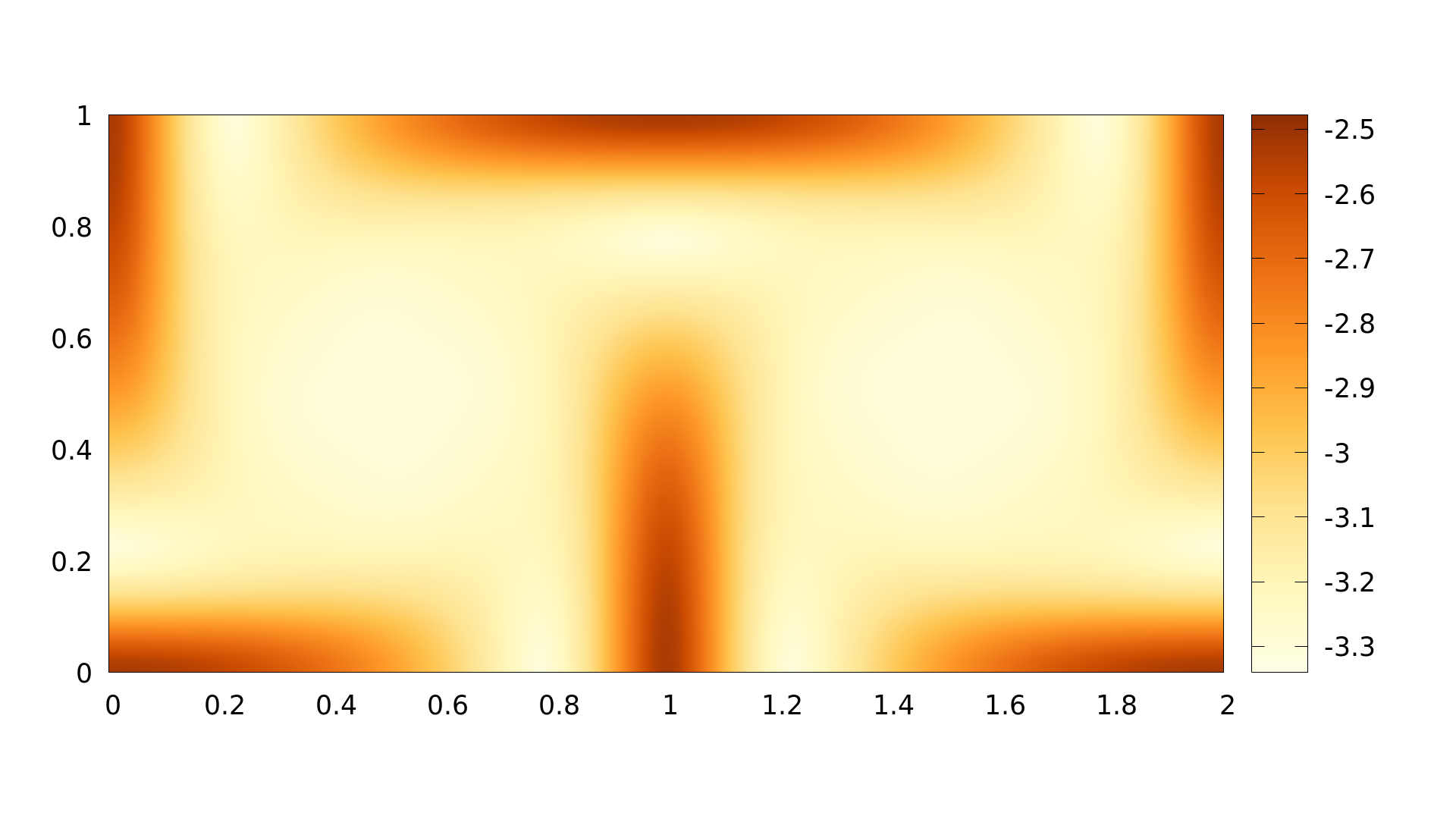
Figure 3: Ensemble $E_{3}$. Left row from top to bottom: FTLE of ensemble runs (all identical).
Right row from top to bottom: D-FTLE, variance of D-FTLE, FTVA.

Figures 1–3 show that standard uncertain FTLE concepts do not give sufficient information to distinguish different sources of uncertainty of FTLE ridges. This is the motivation for introducing our new approach.

5 Overview of our method

Given an ensemble of velocity fields ${{\mathbf{v}}}_{1},...,{{\mathbf{v}}}_{n}$ with the corresponding flow maps $\phi_{1},...,\phi_{n}$, our method consists of the following algorithmic steps:

1. Median flow. We find the ensemble index $m\in\{1,\dots,n\}$ such that $\phi_{m}$ is the best representative of the flows $\phi_{1},\dots,\phi_{n}$. We select $\phi_{m}$ with the lowest sum of all squared point-wise distances to every other flow map. We call $\phi_{m}$ the median flow.
   

2. Computation of domain displacements. We compute a domain displacement for each pair of the median and the ensemble member.

   $${{\mathbf{p}}}_{m,i}:D\times T\times T~{}\to~{}{{\mathbb{R}}}^{q}$$

   that maps points $({{\mathbf{x}}},t)$ to displaced points $({{\mathbf{x}}}^{\prime},t)$ with

   $${{\mathbf{x}}}^{\prime}~{}=~{}{{\mathbf{x}}}+{{\mathbf{p}}}_{m,i}({{\mathbf{x}}},t,\tau)~{}\in~{}D~{}.$$

   Note that the displaced points ${{\mathbf{x}}}^{\prime}$ stay within the domain.
   

   $$\psi_{i}=\phi_{i}({{\mathbf{x}}}^{\prime},t,\tau)$$

   We expect the displacement ${{\mathbf{p}}}_{m,i}$ to be of small magnitude and smooth, and it should align the FTLE ridges of $\phi_{m}({{\mathbf{x}}},t,\tau)$ as much as possible to the FTLE ridges of $\phi_{i}({{\mathbf{x}}}^{\prime},t,\tau)$.
   

3. Computation of displaced flow maps and displaced FTLE. We apply the domain displacements on the corresponding flow maps such that they align with the median flow map. The flow map $\phi_{i}$ is displaced to “match” the median flow. We denote this displaced flow map $\psi_{i}$. We can compute gradients and FTLE from the displaced flow maps $\psi_{i}$. Due to the construction of the domain displacements, we expect the “displaced” FTLE ridges of $\psi_{i}$ to be aligned as much as possible with the FTLE ridges of the median $\psi_{m}=\phi_{m}$.
   

4. Visual analysis. The visual analysis consists of two parts. Firstly, a visualization of the distribution of displaced flow maps $\psi_{i}$, their gradients and their FTLE fields using existing approaches from the literature to visualize the distributions in $(\ref{eq_existingapproaches})$. Secondly, we conduct a visual analysis of the distribution of the domain ${{\mathbf{p}}}_{m,1},\dots,{{\mathbf{p}}}_{m,n}$, which captures information about the uncertainty of both the location and strength of the FTLE ridges.

6 Details of our method

In the following, we present the steps of our method in detail. For a concise notation, we may omit the arguments $t,\tau$ whenever they can be regarded as constants.

6.1 Selection of the median flow $\phi_{m}$

We select the index $m$ of the median flow $\phi_{m}$ as the minimizer of the sums

$$m=\underset{i}{\operatorname*{arg\,min}}\left\{\sum_{j=1}^{n}\int_{D}\mathopen{}\left|\left|{\phi_{i}-\phi_{j}}\parbox[h][0.0pt]{0.0pt}{}\right|\right|^{2}\mathop{}\!\mathrm{d}{{\mathbf{x}}}~{}|~{}i=1,\dots,n\right\}$$

This means that we choose $\phi_{m}$ so that the sum of squared distances for all flows to $\phi_{m}$ becomes minimal.

6.2 Computation of the displacement ${{\mathbf{p}}}_{m,i}$

The objective of the domain displacement function ${{\mathbf{p}}}_{m,i}$ is aligning the FTLE ridges of $\phi_{m}$ as much as possible with the ridges of the flow $\phi_{i}$. To characterize the best alignment of $\phi_{m}$ and $\phi_{i}$, we define the energy

$$A({{\mathbf{p}}})=\frac{1}{\mbox{area}(D)}\int_{D}\mathopen{}\left|\left|{\phi_{m}({{\mathbf{x}}}+{{\mathbf{p}}}({{\mathbf{x}}}))-\phi_{i}({{\mathbf{x}}})}\parbox[h][0.0pt]{0.0pt}{}\right|\right|^{2}_{2}\;d{{\mathbf{x}}}~{},$$

which measures the deviation of the displaced flow map $\phi_{m}$ from $\phi_{i}$ for varying a displacement function ${{\mathbf{p}}}$. In addition, the transformation $({{\mathbf{x}}}+{{\mathbf{p}}}_{m,i})$ should be as rigid as possible: $({{\mathbf{x}}}+{{\mathbf{p}}}_{m,i})$ is rigid if

$$(\nabla({{\mathbf{x}}}+{{\mathbf{p}}}_{m,i}))^{T}\;(\nabla({{\mathbf{x}}}+{{\mathbf{p}}}_{m,i}))={{\mathbf{I}}}~{},$$

which requires (due to $\nabla{{\mathbf{x}}}\neq{{\mathbf{0}}}$)

$$\nabla{{\mathbf{p}}}_{m,i}^{T}\;\nabla{{\mathbf{p}}}_{m,i}+\nabla{{\mathbf{p}}}_{m,i}^{T}+\nabla{{\mathbf{p}}}_{m,i}={{\mathbf{0}}}.$$

We capture this in a second energy term

$$B({{\mathbf{p}}})=\frac{1}{\mbox{area}(D)}\int_{D}\mathopen{}\left|\left|{\nabla{{\mathbf{p}}}^{T}\;\nabla{{\mathbf{p}}}+\nabla{{\mathbf{p}}}^{T}+\nabla{{\mathbf{p}}}}\parbox[h][0.0pt]{0.0pt}{}\right|\right|^{2}_{F}\;d{{\mathbf{x}}}~{},$$

Where $\mathopen{}\left|\left|{\cdot}\parbox[h][0.0pt]{0.0pt}{}\right|\right|_{F}$ denotes the Frobenius norm of a matrix. Depending on the application, we may also consider the additional boundary condition

$$\delta D+{{\mathbf{p}}}_{m,i}(\delta D)=\delta D$$ (2)

where $\delta D$ denotes the boundary of $D$. (2) ensures that a point on the boundary of $D$ is mapped to (another) boundary point of $D$.

We minimize a blend of the alignment term $A$ and the “rigidity” term $B$ to determine the optimal domain displacement as

$${{\mathbf{p}}}_{m,i}=\underset{{{\mathbf{p}}}}{\operatorname*{arg\,min}}~{}(1-\rho)\;A({{\mathbf{p}}})+\rho\;B({{\mathbf{p}}})$$ (3)

for a weight $\rho\in[0,1]$. Note that for the extreme cases $\rho=0$ and $\rho=1$, (3) has a closed-form minimizer: For $\rho=1$ the trivial minimizer is

$${{\mathbf{p}}}_{m,i}={{\mathbf{0}}}$$ (4)

For $\rho=0$, the function

$${{\mathbf{p}}}_{m,i}=\phi_{m}\left(\phi_{i}({{\mathbf{x}}},\,t,\,\tau),\,t+\tau,\,-\tau\right)-{{\mathbf{x}}}$$ (5)

yields $A({{\mathbf{p}}}_{m,i})=0$ and this minimizes (3)). This minimizer (5) is obtained as follows: for each location and time $({{\mathbf{x}}},t)$, we first integrate ${{\mathbf{v}}}_{j}$ over a period $\tau$. From the resulting point $\phi_{i}({{\mathbf{x}}},t,\tau)$, we apply a backward integration of ${{\mathbf{v}}}_{m}$ over the negative period $-\tau$.

Note that neither (5) nor (4) are useful solutions: (5) is perfectly rigid but has no effect, and while (5) maximizes the alignment of $\phi_{m}$ and $\phi_{i}$, it also tends to have strong gradients (which grow exponentially in $\tau$) and can therefore neither expected to be small nor smooth. Instead, we search for a solution of (3) for a parameter $0<\rho<1$ that keeps ${{\mathbf{p}}}_{m,i}$ small and smooth while simultaneously aligning the ridges. The influence of the parameter $\rho$ is discussed in section 8 and figure 16.

Minimizing (3) is a nonlinear optimization problem. We describe the discretization and the numerical solution in section 6.5

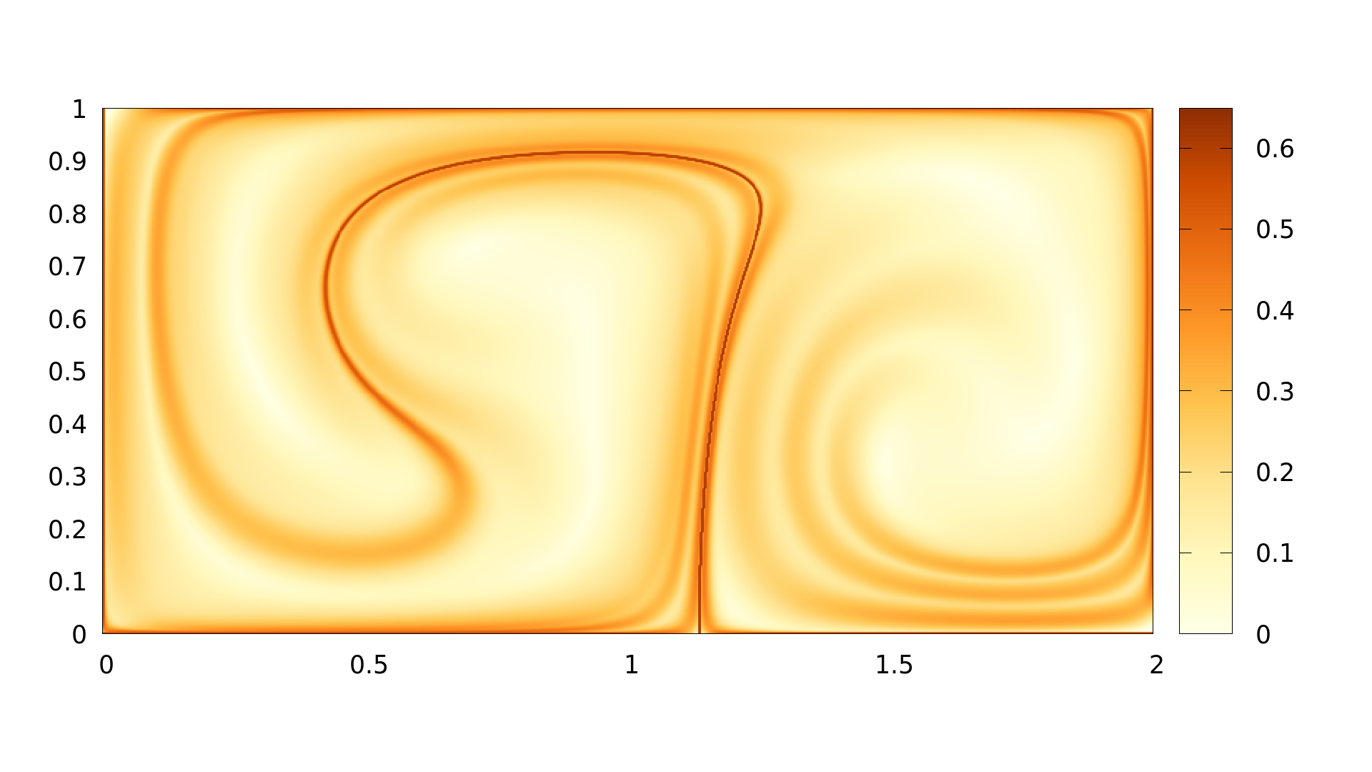
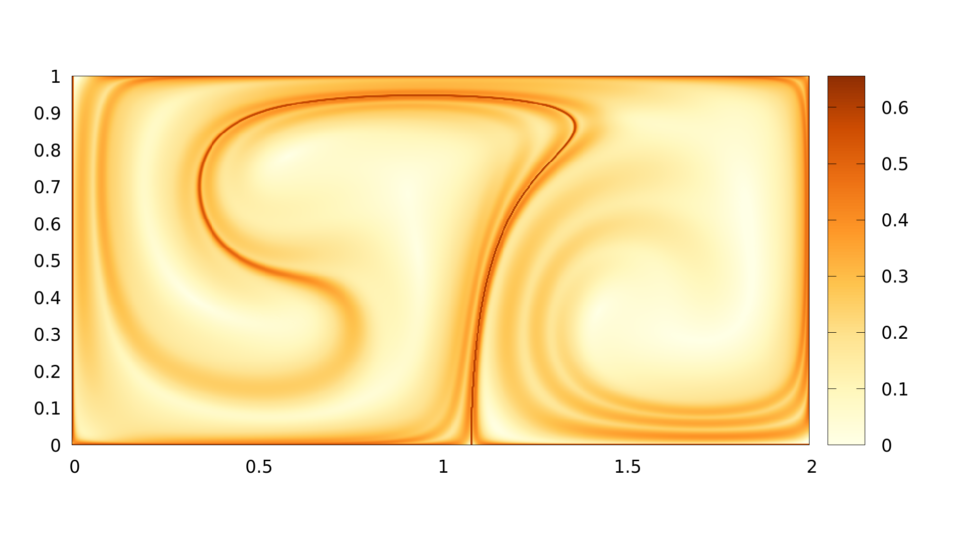
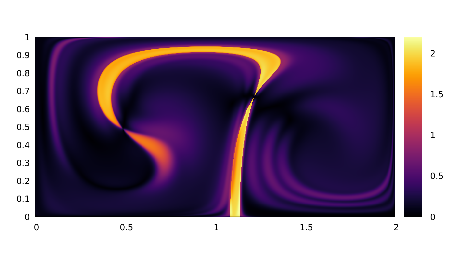
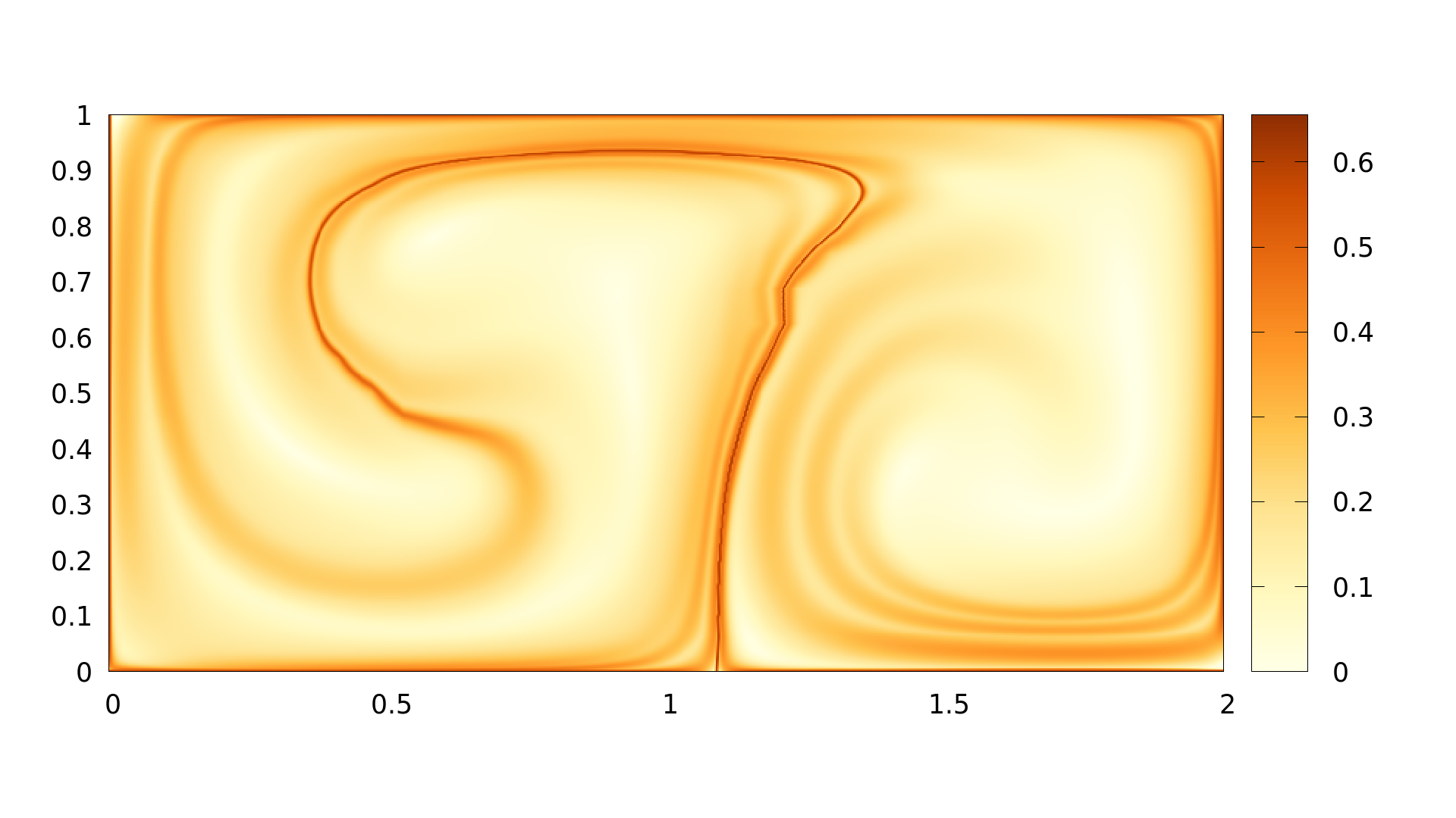
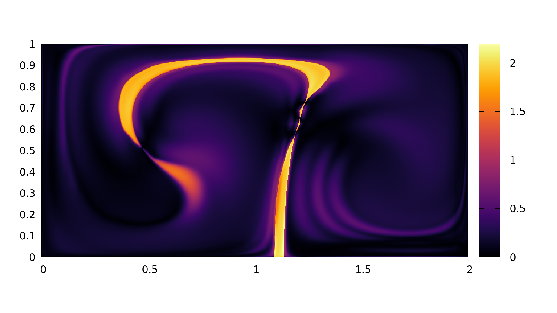
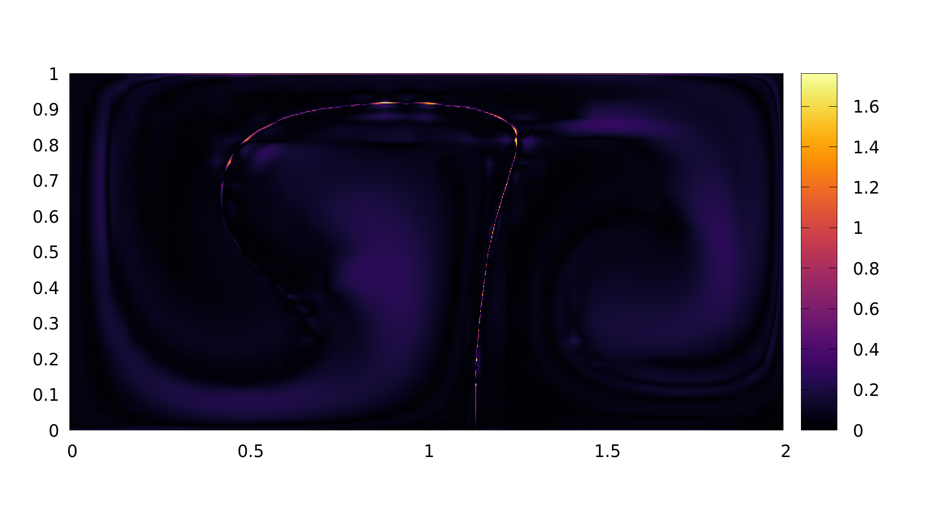
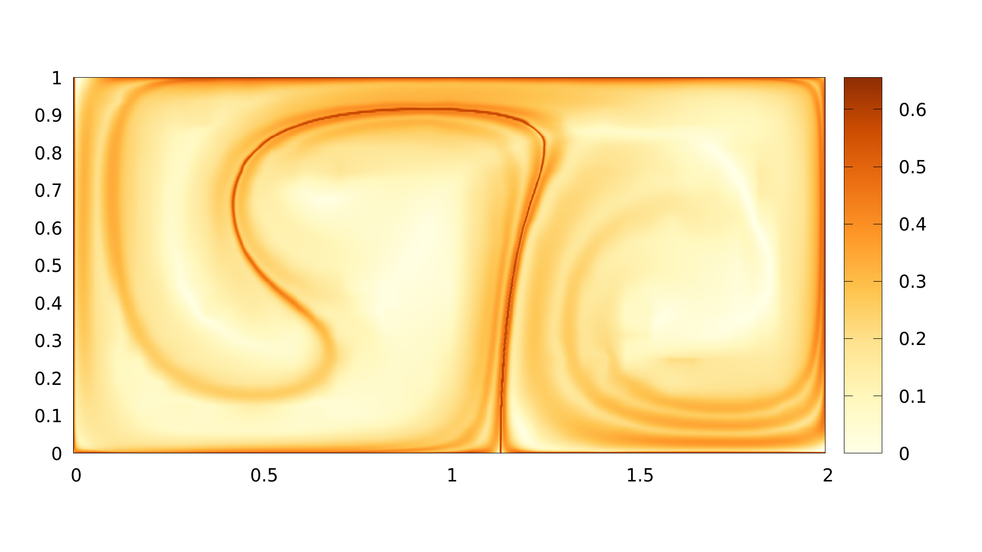
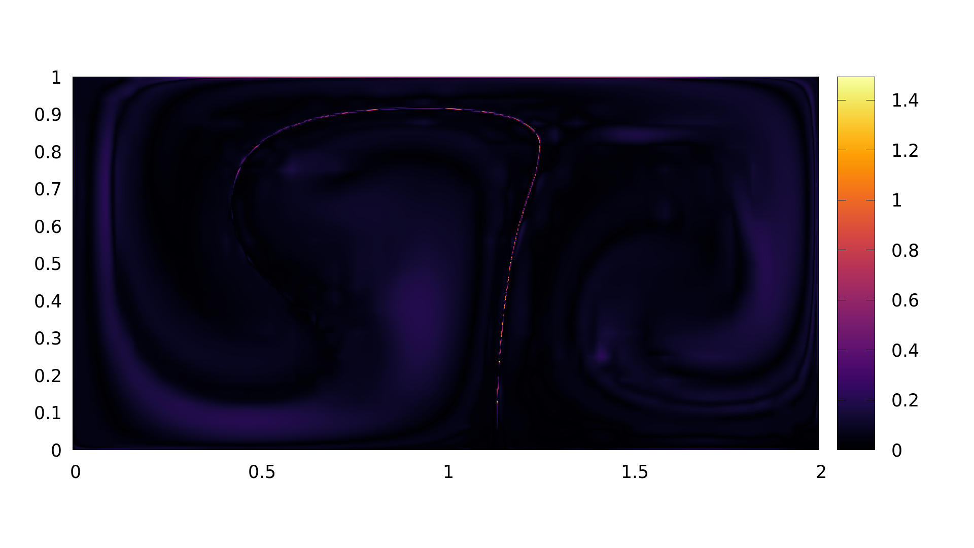
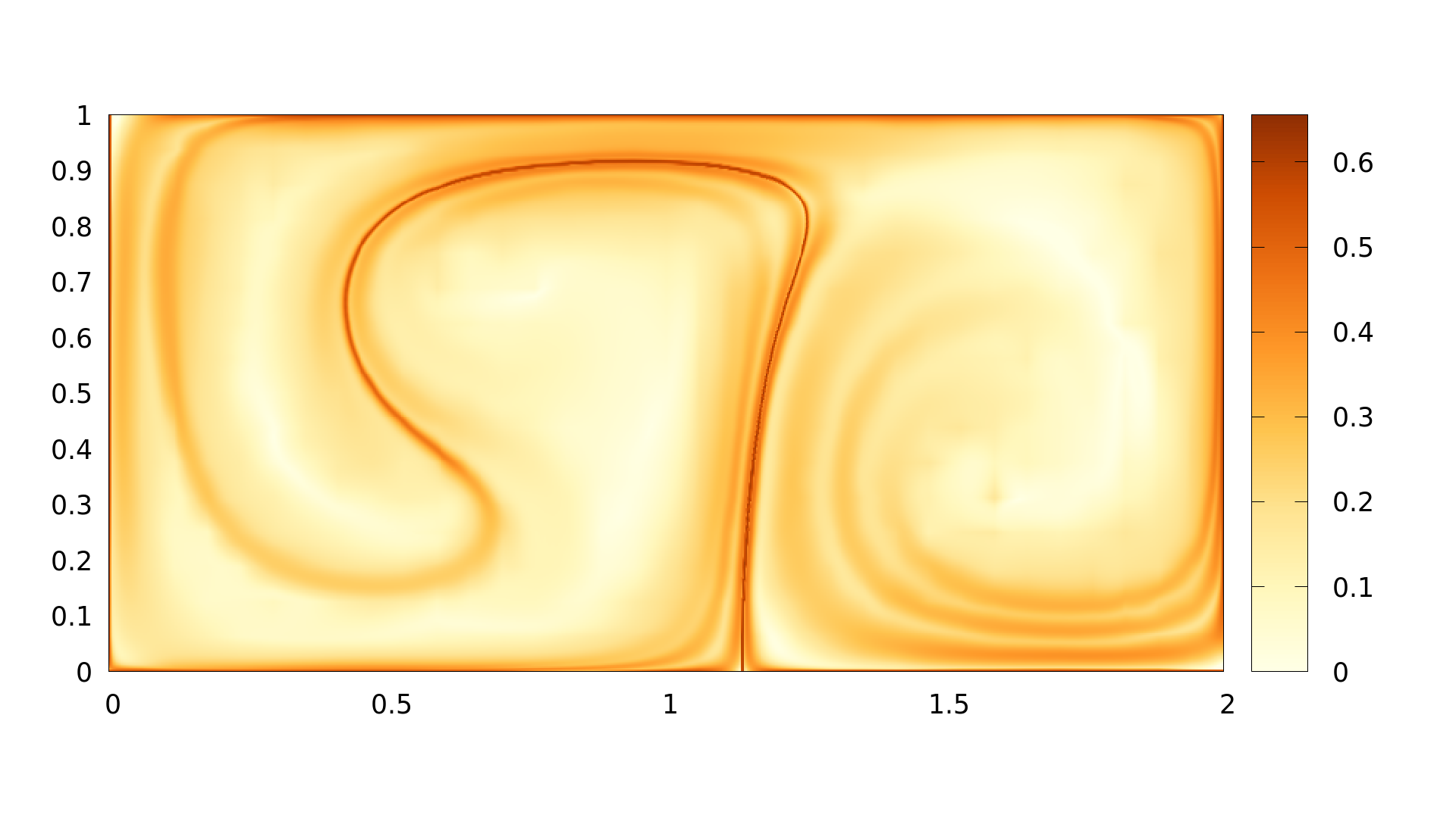
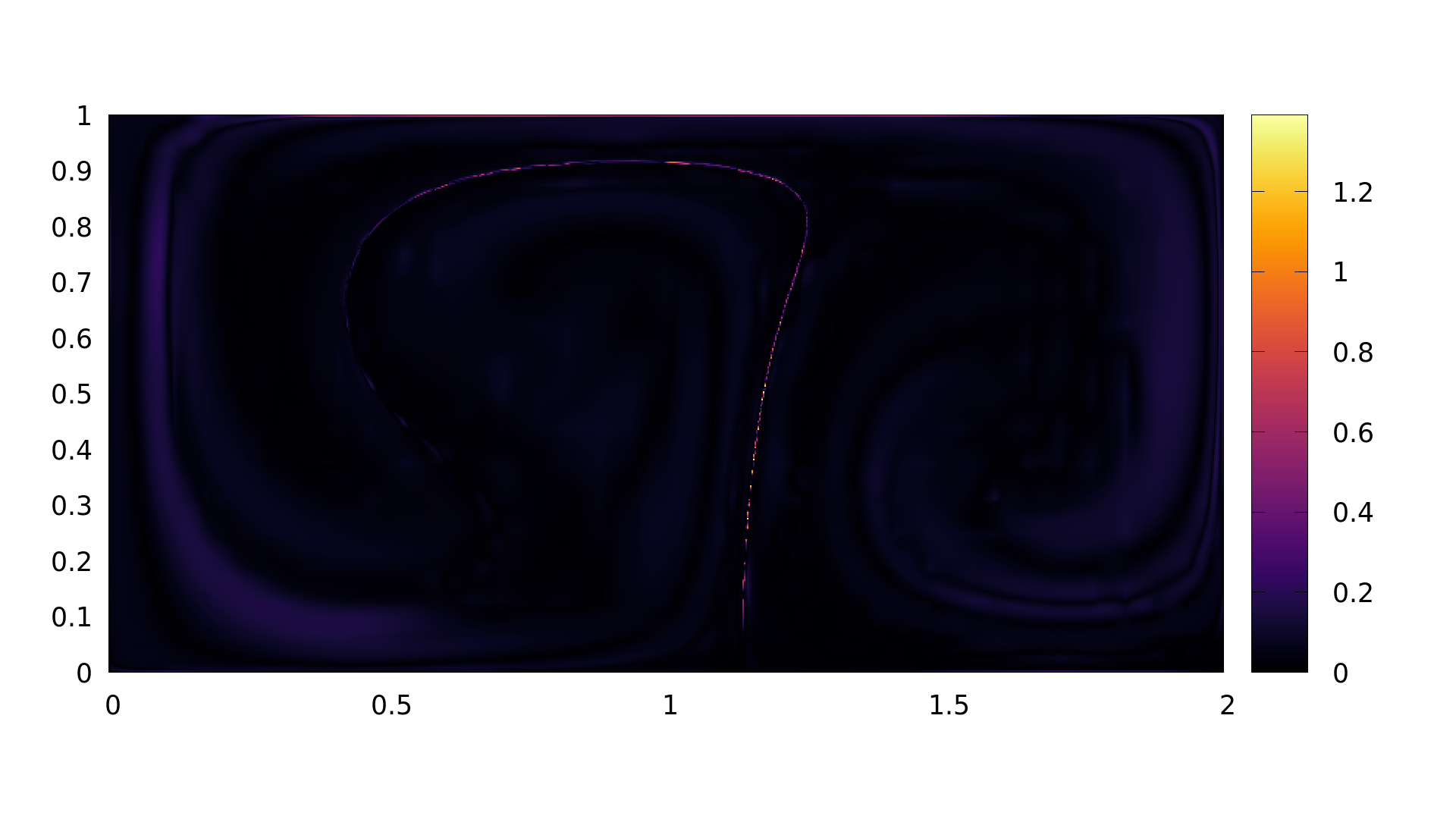
Figure 4: Optimization for alignment of 2 Double Gyre ensembles. Top row (from left): two ensemble members and energy $A({{\mathbf{p}}})$ to be minimized.
Rows 2–5 show the state of optimization after 7, 46, 99 and 151 iterations. Each row shows (from left): ${{\mathbf{p}}}$, $\overline{\mbox{FTLE}}$, $A({{\mathbf{p}}})$.

6.3 Displaced flow maps and displaced FTLE.

For each ensemble member $i=1\dots,n$, we compute the displaced flow map

$$\psi_{i}({{\mathbf{x}}},t,\tau)=\phi_{i}({{\mathbf{x}}}+{{\mathbf{p}}}_{m,i}({{\mathbf{x}}},t,\tau),t,\tau)~{}.$$ (6)

We can compute the (spatial) gradient

$$\nabla\psi_{i}({{\mathbf{x}}},t,\tau)=\nabla\phi_{i}({{\mathbf{x}}}+{{\mathbf{p}}}_{m,i}({{\mathbf{x}}},t,\tau),t,\tau)\;\left({{\mathbf{I}}}+\nabla{{\mathbf{p}}}_{m,i}({{\mathbf{x}}},t,\tau)\right)$$ (7)

where ${{\mathbf{I}}}$ denotes the identity. Based on $\nabla\psi_{i}$, we define displaced FTLE

$$\overline{\mbox{FTLE}}_{i}({{\mathbf{x}}},t,\tau)=\frac{1}{|\tau|}\ln\sqrt{\lambda_{\max}\left((\nabla\psi_{i})^{T}\,\nabla\psi_{i}\right)}~{}.$$ (8)

Note again that the idea behind the displacement ${{\mathbf{p}}}_{m,i}$ is to align the ridges of $\overline{\mbox{FTLE}}_{i}$ with the ridges of $\overline{\mbox{FTLE}}_{m}$ as close as possible , i.e., the ridges of the median flow. Remarks:

• (6) shows that $\psi_{i}$ is not obtained by integrating a new velocity field. Instead, $\psi_{i}$ is obtained by a deformation of the precalculated flow map $\phi_{i}$ with the domain displacement ${{\mathbf{p}}}_{m,i}$.

• (7) shows the relation between the gradients of $\phi_{i}$ and $\psi_{i}$. In particular, it shows that $\nabla\phi_{i}$ only becomes extremal if either $\nabla\psi_{i}$ or $\nabla{{\mathbf{p}}}_{m,i}$ become extremal. Since the condition $B({{\mathbf{p}}}_{m,i})$ prevents $\nabla{{\mathbf{p}}}_{m,i}$ from becoming extremal and keeping in mind that FTLE is based on considering the extremals in $\phi_{i}$ and $\psi_{i}$ respectively, there is a one-to-one relation between the ridges of $\nabla\phi_{i}$ and $\nabla\psi_{i}$. Therefore, our alignment approach cannot produce new FTLE ridges or make existing ones disappear. It can only transform and align their locations.

6.4 Visual analysis and interpretation

Visual analysis can be based on either of

$$\psi_{1},\dots,\psi_{n}\quad\textbf{or}\quad\nabla\psi_{1},\dots,\nabla\psi_{n}\quad\textbf{or}\quad\overline{\mbox{FTLE}}_{1},\dots,\overline{\mbox{FTLE}}_{n}~{}.$$

For the visualization of $\psi_{1},\dots,\psi_{n}$, we apply existing techniques for uncertain FTLE visualization: D-FTLE and FTVA.

In addition, we can visually analyze the distribution of the domain displacements ${{\mathbf{p}}}_{m,i}$. This provides information about the uncertainty of both, the location and the strength of FTLE ridges. Assuming a normal distribution of all ${{\mathbf{p}}}_{m,i}$, we analyze the covariance

$${{\mathbf{C}}}({{\mathbf{x}}},t,\tau)=\frac{1}{n}\sum_{i=1}^{n}\,{{\mathbf{p}}}_{m,i}({{\mathbf{x}}},t,\tau)\,\,{{\mathbf{p}}}_{m,i}({{\mathbf{x}}},t,\tau)^{T}~{}.$$ (9)

Assume that the integration time $t$ and period $\tau$ are fixed. Then the tensor field ${{\mathbf{C}}}$ assigns a symmetric positive definite matrix to every domain point ${{\mathbf{x}}}$ . For a given direction vector ${{\mathbf{r}}}$ with $\mathopen{}\left|\left|{{{\mathbf{r}}}}\parbox[h][0.0pt]{0.0pt}{}\right|\right|=1$, the quadratic form ${{\mathbf{r}}}^{T}\,{{\mathbf{C}}}\,{{\mathbf{r}}}$ measures the variance of the domain displacements in this direction. We are interested in the variances near FTLE ridges: high variance in a direction perpendicular to a ridge indicates a high uncertainty in ridge location, whereas high variance in a direction parallel to a ridge indicates high uncertainty in the strength of separation. The case ${{\mathbf{C}}}={{\mathbf{0}}}$ indicates that the ridges of all ensemble members are perfectly aligned and have similar strength.

This tool complements the analysis of the distribution of $\overline{\mbox{FTLE}}$: Visualizing $\overline{\mbox{FTLE}}_{1},\dots,\overline{\mbox{FTLE}}_{n}$ gives information about the average strength of separation, while the analysis of ${{\mathbf{C}}}$ reveals the uncertainty of ridge location and strength.

We visualize the tensor field ${{\mathbf{C}}}$ by placing non-overlapping ellipses. We are therefore computing the corresponding ellipse for every FTLE value above a certain FTLE value. As higher FTLE values tend to be close to each other, ellipses would overlap. We therefore prioritize ellipses with corresponding higher FTLE values in a case of overlapping. In order to prevent occluding the LCS structures, the ellipses are rendered semi-transparent. This reduces clutter while preserving to render ellipses on the more important regions. Ellipses below a certain diameter will also be discarded to prevent the clutter of dots on ridges with a high certainty. High FTLE values which are not covered by ellipses therefore have a high certainty. The scale of the ellipses is chosen as the 95 percentile of the normal distribution. Figures 6 and 7 show examples. Based on this, we observe the extent and orientation of the ellipses along the ridges of the underlying uncertain FTLE fields, which gives the following interpretation:

• The width and sharpness of a ridge indicate the strength of separation: the sharper the ridge, the stronger the flow separation.

• The uncertainty in the strength of separation is encoded in expansion of the ellipses in the direction of the ridge: large expansion in ridge direction corresponds to high uncertainty in the strength of separation along the ridge.

• The uncertainty in the ridge location is encoded in the ellipse expansion in the direction perpendicular to the ridges: the larger the ellipse expansion perpendicular to the ridge is, the more uncertain the ridge locations.

Figure  5 illustrates the interpretation of uncertain ridges.

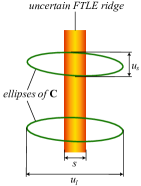
Figure 5: Sources of uncertainty encoded by our approach using tensors ${{\mathbf{C}}}$ (see (9)): The width $s$ of a ridge corresponds to the strength of separation. The expansion $u_{s}$ of the ellipse parallel to the ridge encodes uncertainty of the strength of separation. Expansion $u_{l}$ perpendicular to the ridge encodes uncertainty of ridge location.

6.5 Numerical optimization

We sample flow maps $\phi_{i}$ for all ensemble members and compute pairwise distances to select the median flow map. As the flow maps are sampled on a regular grid and represented as matrices, we measure the distance between two flow maps $i,j$ simply as $invn{\phi_{i}-\phi_{j}}_{F}$. Then the main task is finding an optimal displacement $p_{i,m}$ for each flow field $\phi_{i}$ w.r.t. the median flow $\phi_{m}$ as outlined in section 6.2.

We represent domain displacements as bilinear maps $D\to{}D$, which are parameterized by a grid of nodes or control points in 2d. For each map we can evaluate the cost function (3) by replacing the integrals in the terms $A$ and $B$ by discrete sums. Note that this summation acts on the discrete flow map, i.e., in the sampling resolution. We use the L-BFGS algorithm, a quasi-Newton method, for minimizing the cost function. This requires also the evaluation of the gradient of the cost function. We use central differences for approximating the gradient an the following observation for avoiding redundant computations: The displacement map is defined using a bilinear basis functions with compact support, i.e., each control points acts only on a neighborhood w.r.t. to the control grid. This is a well-known property: our setting is a simple case of a tensor product B-splines.

For the estimation of a partial derivative w.r.t one node using a finite difference, this means that the summation (i.e., the discrete integration) can be restricted to a local neighborhood: as all contributions away from this neighborhood stay constant, they cancel in the finite difference. Note that a similar argument applies in a continuous formulation.

As the gradient estimation dominates the computational cost for minimization, this observation has a significant impact on performance, because it “decouples” the resolution of the sampling grid from the resolution of the grid of nodes controlling the displacement: The computation cost is de facto bound by the significantly lower resolution of the control grid. For additional speedup, we take advantage of parallel computation for both, the summation over the whole domain for evaluation the cost function and for the evaluation of partial derivatives.

We apply the following boundary conditions for the minimization: all nodes must stay within the domain, and displacements – i.e., nodes – on the boundary must map to a boundary point, i.e., they have only one degree of freedom along the boundary curve. This ensures that the displaced points stay within the domain. Displacements at the corners of the rectangular domain vanish: corners remain corners. Note that the latter condition is only meaningful if there are feature points such as corners on the domain boundary curve (e.g., for a rectangle).

Note that the term $B({{\mathbf{p}}})$ that penalizes nonrigid behavior enforces a smooth displacement and to some extent penalized non-bijective displacements maps, i.e., “flipped” cells in the deformed grid. We don’t see any need to add further constraints that guarantee a bijective deformation of the domain (see also section ).

Finally, the computations required for the visual analysis and interpretation (section 6.4), are straightforward: replace $\phi_{i}$ by $\psi_{i}$. We sample $\psi_{i}$ for computing $\nabla\psi_{i}$ and $\overline{\mbox{FTLE}}$ similarly as for computing $\nabla\phi_{i}$ and FTLE from sampled flow maps $\phi_{i}$.

7 Results

7.1 Introductory example

We start the analysis of our method in comparison to the introductory example in section 4, previously illustrated in figures 1–3. Figure 6 (top) shows D-FTLE of the optimal domain displaced flow ensemble $\psi_{1},...,\psi_{50}$. We see a rather sharp ridge at the location $x=1$, encoding a strong separation. Further, we see that the ellipses of ${{\mathbf{C}}}$ on the ridges have a strong expansion in the direction perpendicular to the ridge direction, where the expansion parallel to the ridge expansion is low. This encodes the strong uncertainty of ridge location, and weak uncertainty of the strength of separation. Figure 6 (bottom) shows the variance of domain displaced D-FTLE, in comparison to its non-displaced version in figure1 (right column, second row). Figure 7 (top) shows the result for the ensemble $E_{2}$. Here the ellipses of ${{\mathbf{C}}}$ align with the ridge direction, encoding a strong uncertainty of the separation strength but low uncertainty in the ridge location. For reference, compare the variance of the domain displaced D-FTLE figure 7 (bottom) with the variance of the original D-FTLE figure 2 (right column, second row). Figure 8 shows D-FTLE and its variance for the ensemble $E_{3}$. Here, we see no ellipses of ${{\mathbf{C}}}$ at all. In fact, all ellipses are vanishing, indicating no uncertainty in ridge location and strength of separation.

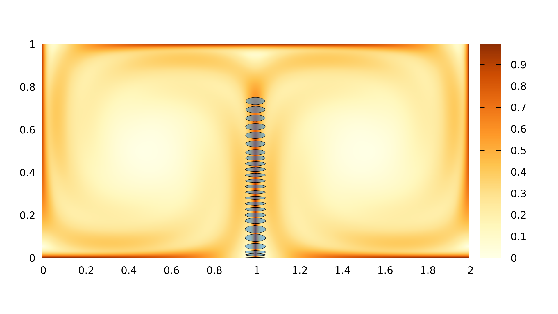
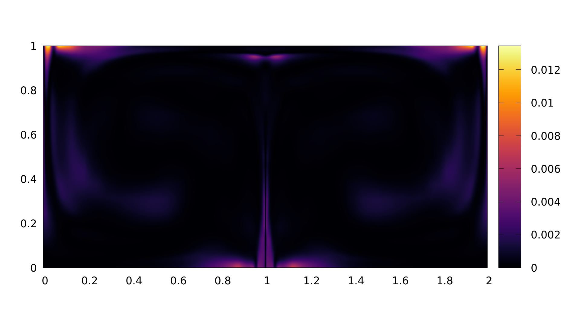
Figure 6: The optimal domain displaced D-FTLE and its variance for ensemble $E_{1}$.

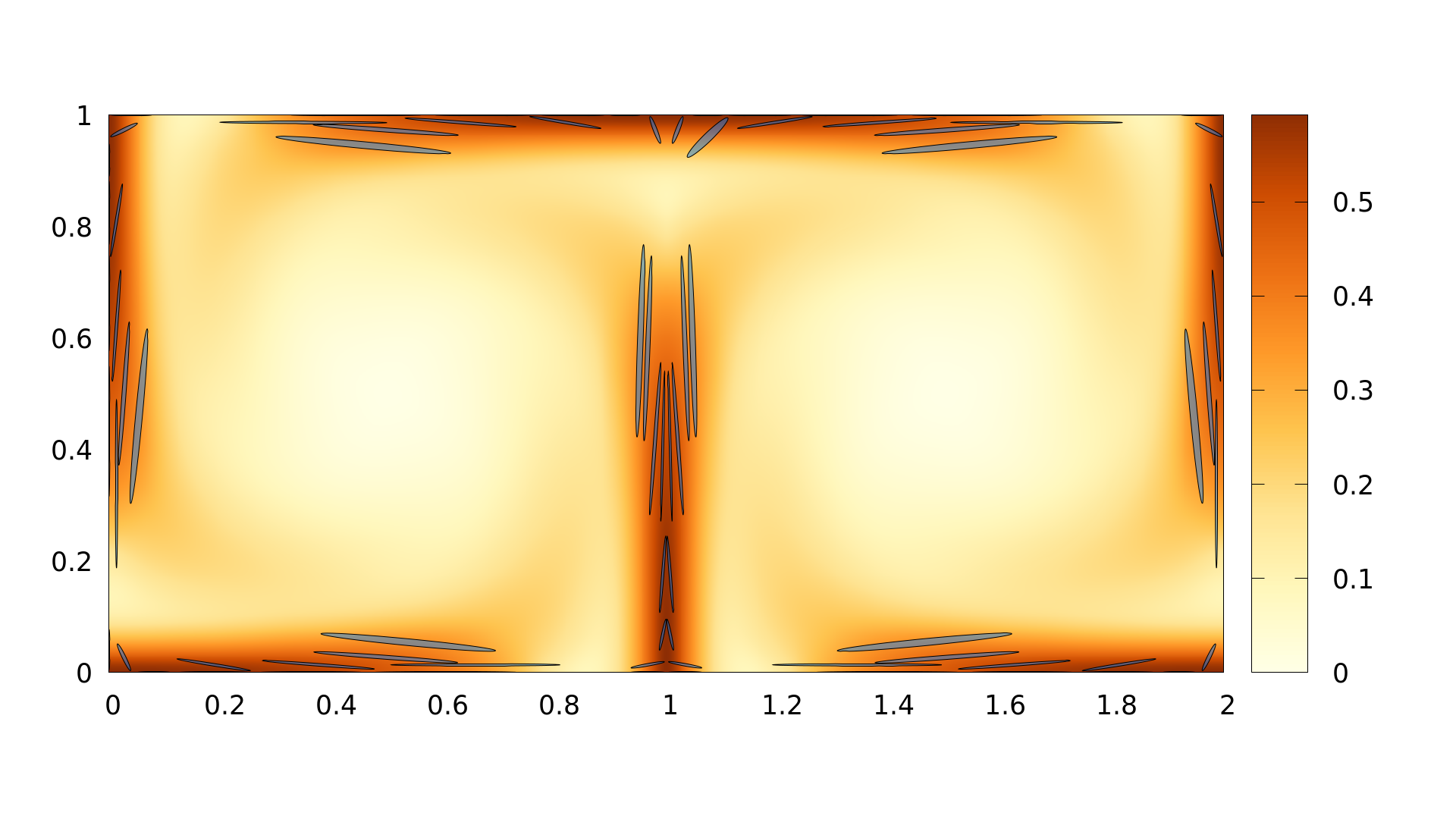
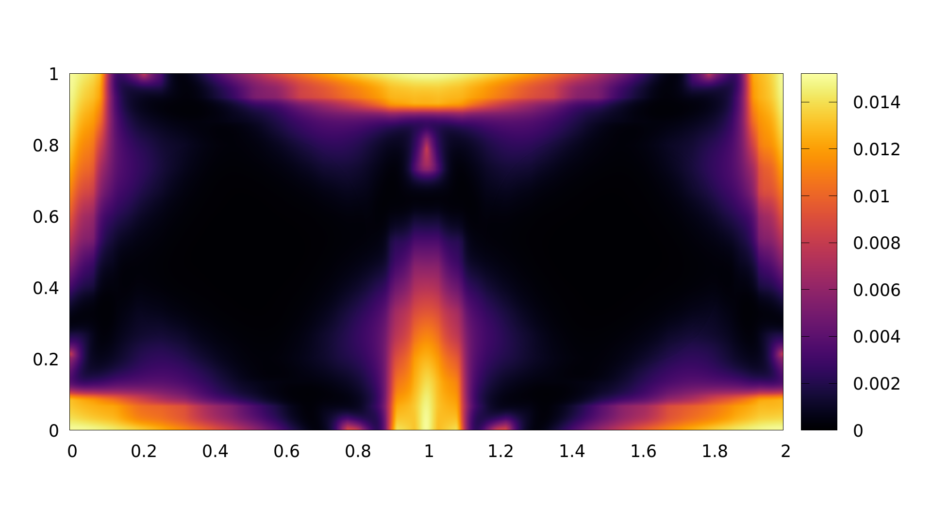
Figure 7: The optimal domain displaced D-FTLE and its variance for the ensemble $E_{2}$.

Figure 8: The optimal domain displaced D-FTLE and its variance for the ensemble $E_{3}$.

7.2 Double gyre

We consider the double gyre data set from [SLM05b] that is defined as

$$f(x,t) = a(t)x^{2}+b(t)x$$ (10)

$$a(t) = \epsilon\,sin(\omega t)$$ (11)

$$b(t) = 1-2\epsilon\,sin(\omega t)$$ (12)

$${{\mathbf{v}}}_{DG}({{\mathbf{x}}},t)={{\mathbf{v}}}_{DG}(x,y,t) = \begin{pmatrix}\pi\,A\,sin(\pi f(x))cos(\pi y)\\ \pi\,A\,cos(\pi f(x))sin(\pi y)\end{pmatrix}$$ (13)

We use $A=0.1$, $\epsilon=0.25$ and $\omega=\frac{2\pi}{10}$. The data set is an interesting test case because we can create different ensemble members by varying $t$ and $\tau$. In fact, varying $t$ results in ridges at different positions, as the Gyres oscillate. Different integration times $\tau$ result in FTLE ridges of different strength and width. Figure 9 shows an ensemble of 50 members with times in the range of $t={-0.5,0.5}$ and constant integration time $\tau=11$ of the Double Gyre.

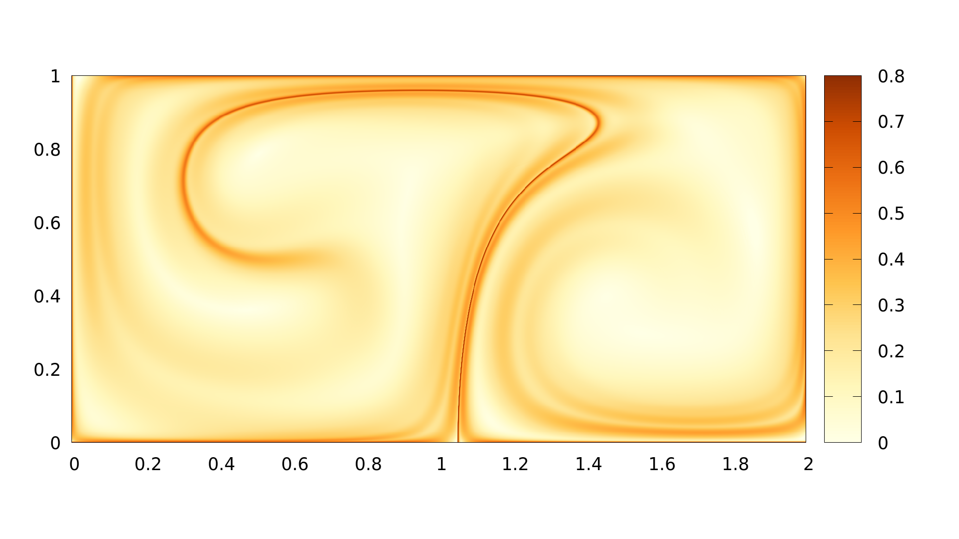
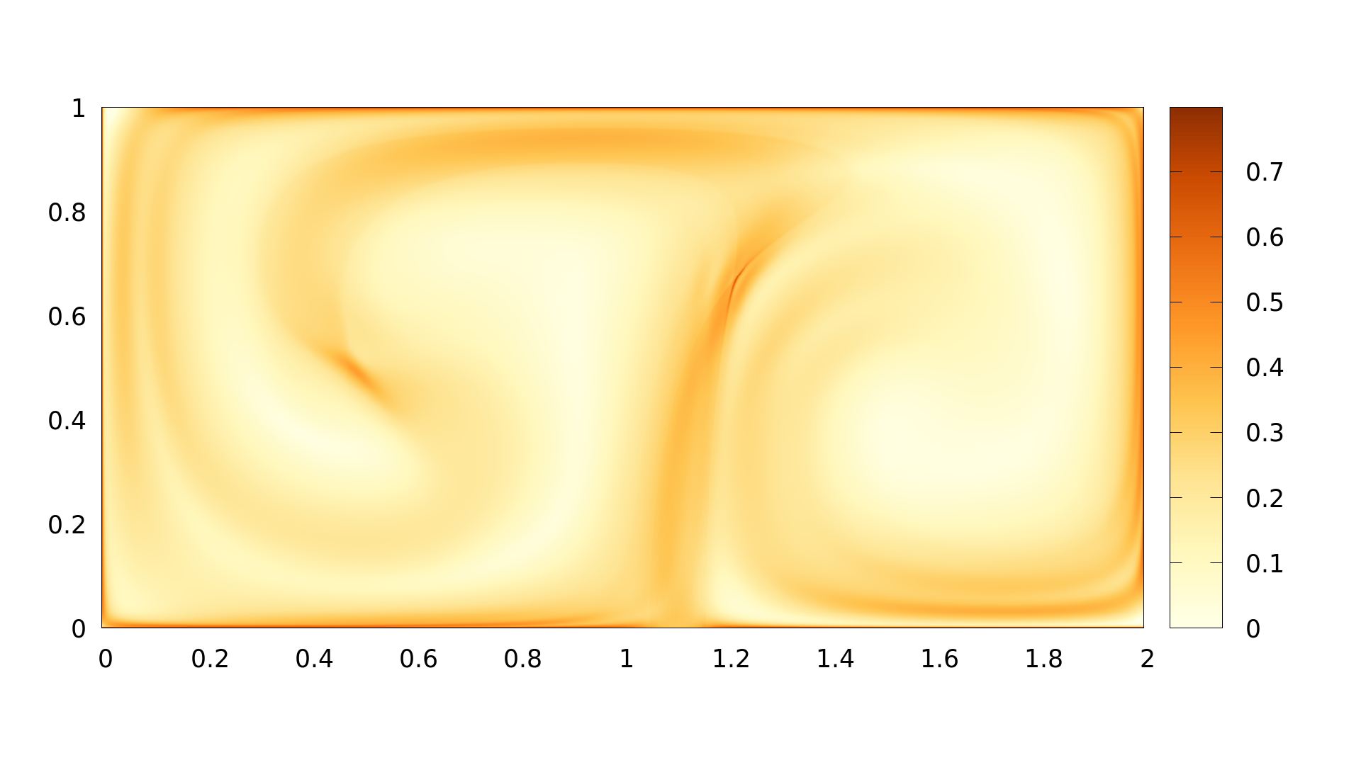
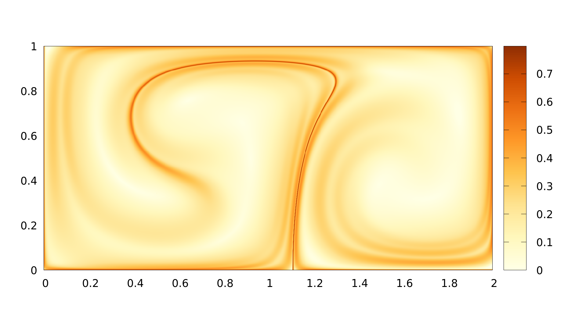
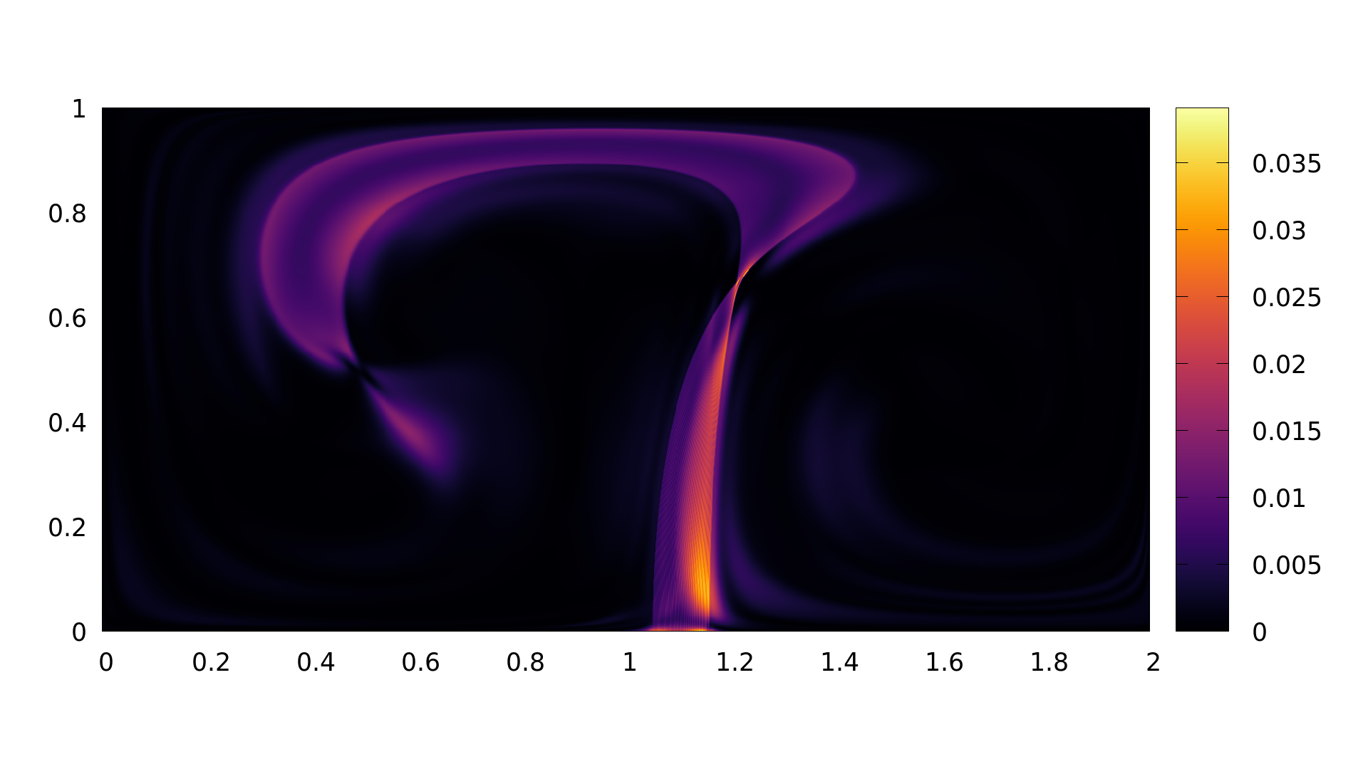
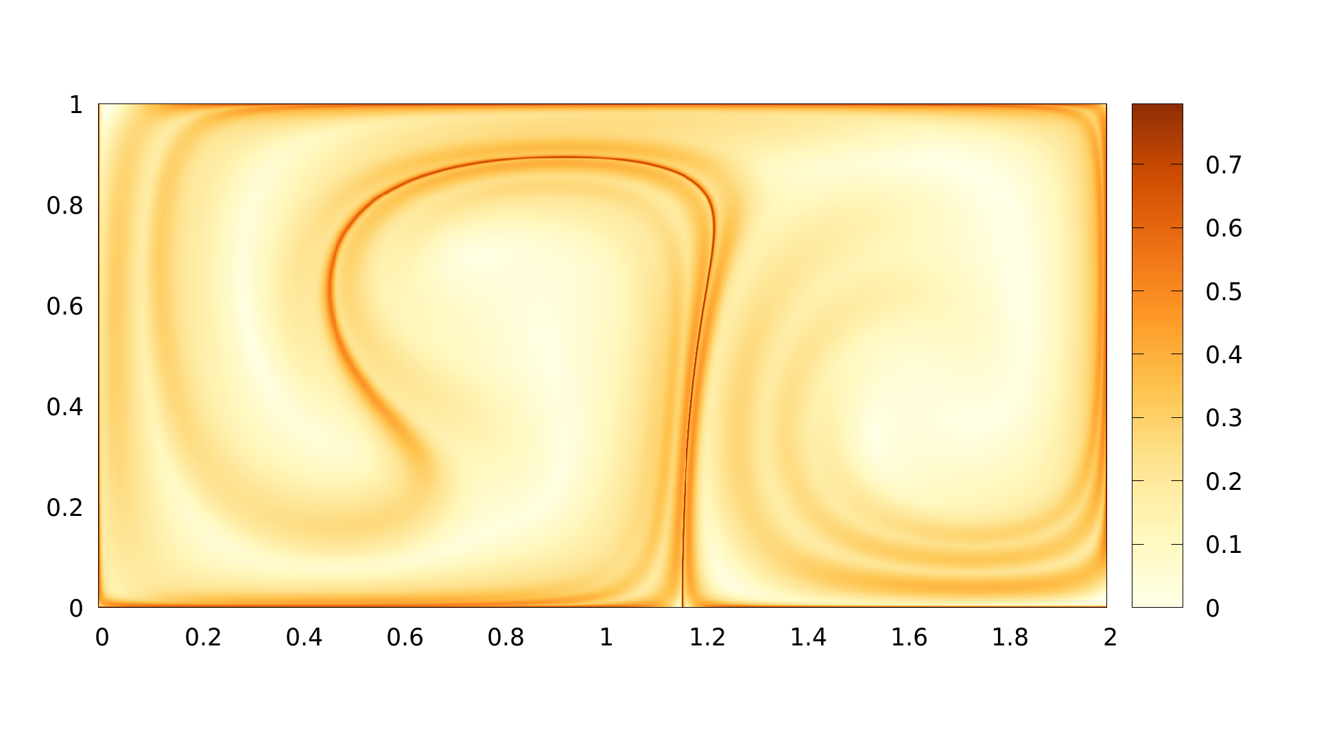
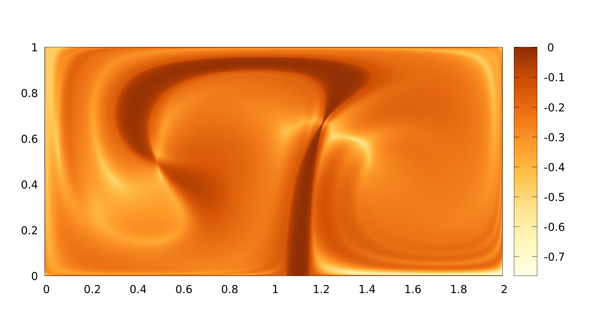
Figure 9: Double Gyre ensemble with $\tau=11$. Left column from top to bottom: FTLE of ensemble runs with $t=-0.5$, $t=0$, $t=0.5$,.
Right column from top to bottom: D-FTLE, variance of D-FTLE, FTVA.

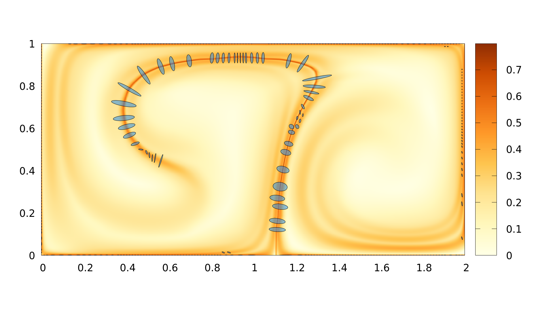
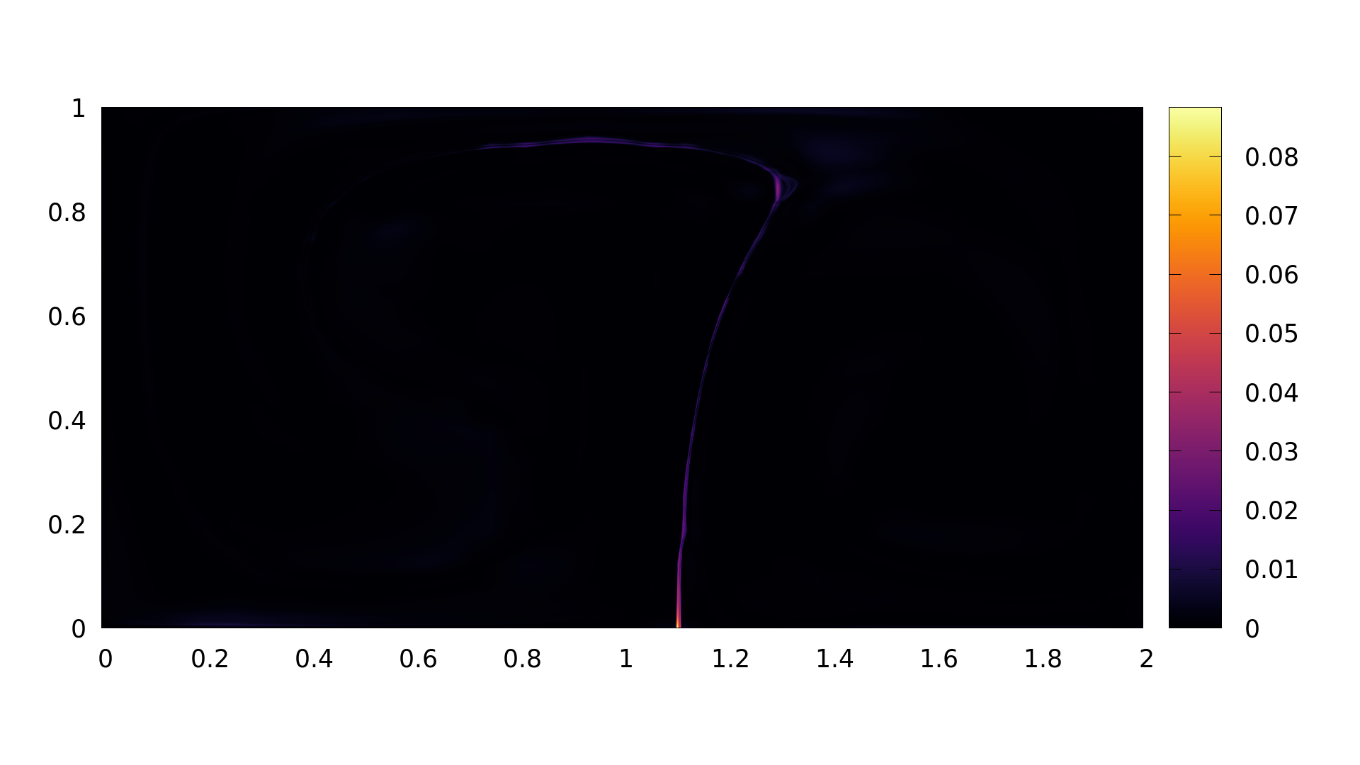
Figure 10: The optimal domain displaced D-FTLE and its variance for the Double Gyre ensemble.

Figure 9(left column) shows the FTLE fields of the ensemble members. The right-hand column of 9 shows standard uncertain FTLE visualizations: D-FTLE, variance of D-FTLE, FTVA (from top to bottom). They show broad and unsharp ridges which are nearly vanishing.
Figure 10 shows the result of our approach: D-FTLE and its variance for the domain displaced ensemble members. We see sharp ridges, encoding a strong separation. Along the ridges we observe different kinds of behavior of the ellipses of ${{\mathbf{C}}}$. In most regions they are rather "thin" (i.e, having a strong aspect ratio). Further, in some regions they are aligned with the ridge directions, while in other parts orientation is perpendicular to the ridge direction.

7.3 Displacement example

To give further insight of the optimal domain displacement, we want to give an example of the Double Gyre optimal domain displacements. Figure 11 shows the difference of the domain alignments along the ensembles. Note that ensembles closer to the median tend to have smaller domain displacements too. The resulting domain displaced FTLE fields are similar to the FTLE field of the selected median flow.

][t]0.22

][t]0.26

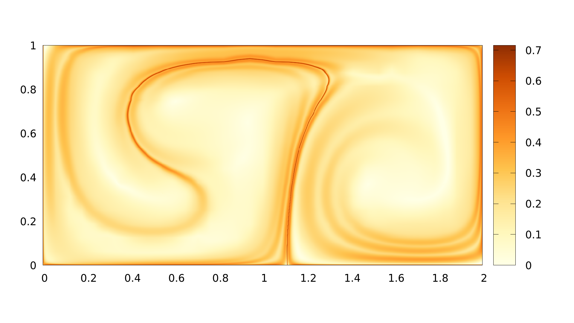
][t]0.22

][t]0.26

][t]0.22

][t]0.26

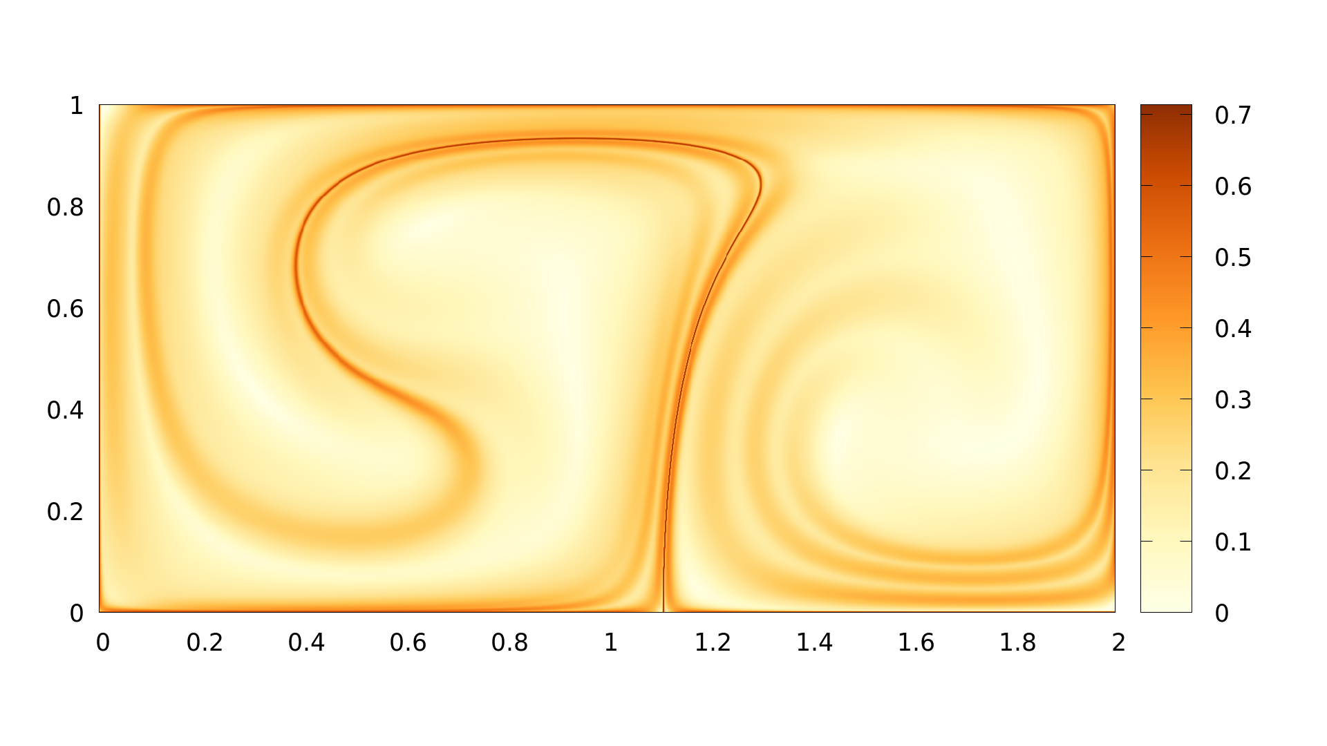
][t]0.22

][t]0.26

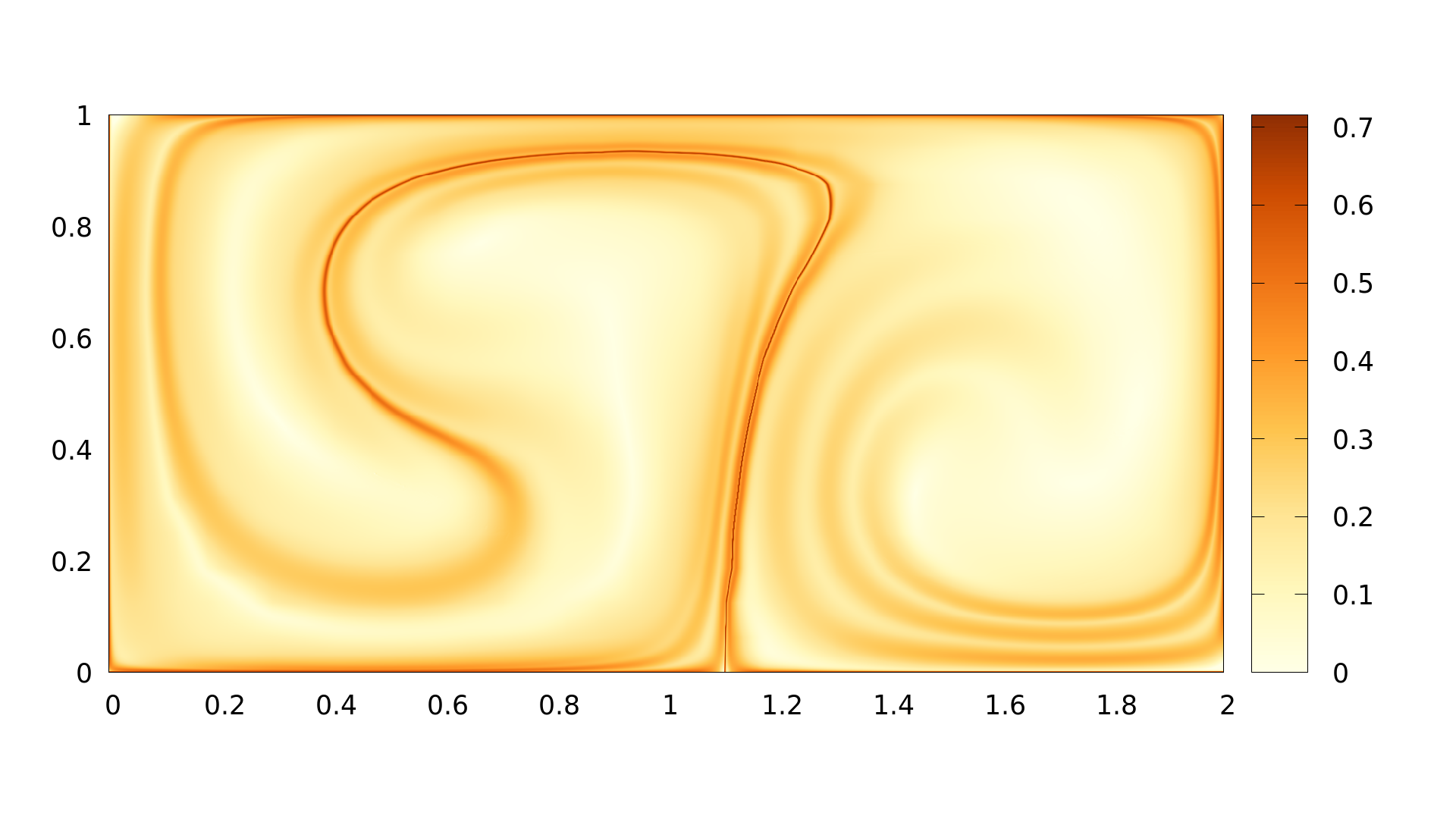
][t]0.22

][t]0.26

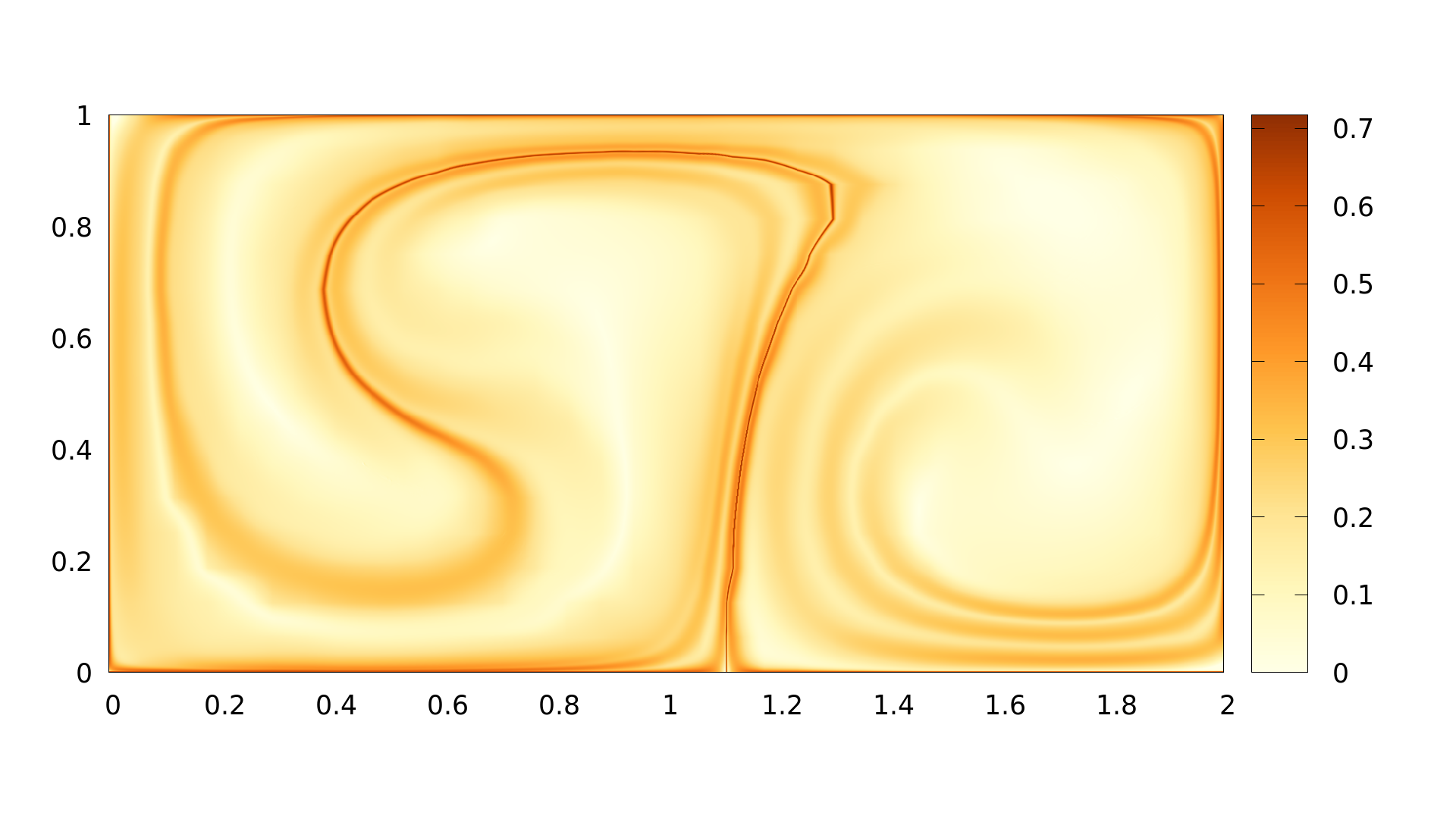
Figure 11: Double Gyre ensemble with $\tau=11$. Left column from top to bottom: Optimal domain displacement onto median flow $\phi_{m}$ with $m=25$ visualized as grid deformation: ${{\mathbf{p}}}_{m,1}$, ${{\mathbf{p}}}_{m,13}$, ${{\mathbf{p}}}_{m,m}$, ${{\mathbf{p}}}_{m,38}$, ${{\mathbf{p}}}_{m,50}$
Right column from top to bottom: Optimal displaced FTLE ensemble member onto median flow 25: $\overline{\mbox{FTLE}}_{1}$, $\overline{\mbox{FTLE}}_{13}$, $\overline{\mbox{FTLE}}_{25}$, $\overline{\mbox{FTLE}}_{38}$, $\overline{\mbox{FTLE}}_{50}$

7.4 Red Sea

We apply our method to all 50 members of the Red Sea Data set from the SCIVis-Contest 2020 [Sci]. In particular, we take a closer look at the south of the Red Sea and the Bab-el-Mandeb strait. Figure 12 shows the FTLE fields of the 4 ensemble members, revealing that the ensembles are quite divers and different in some regions. The red sea has a relative constant inflow through the Bab-el-Mandeb strait, the differences are low in this region along the ensemble members. This can also be observed in the magnified area of the Bab-el-Mandeb strait. This changes drastically for the northern part where ensembles are quite different. Those differences can especially be observed in the magnified northern region of the Red Sea. Some showing low to no seperation at all 12(top left and top right), while other show higher seperation (bottom left) or even eddies (bottom right). We consider this as an extreme case for our approach in trying to find alignments of the ensemble members.

Figure 12: Red Sea ensemble with $\tau=48$ which relates to an integration time of two days. Top row from left to right: FTLE of the Red Sea ensemble data set 1 and 2.
Bottom row from left to right: FTLE of the Red Sea ensemble data set 13 and 16.

Figure 13: Red Sea data set with 50 ensemble members; (top left) D-FTLE revealing different kind of ridges; (top right) D-FTLE of the domain displaced ensemble members gives slightly sharper ridges than (top left) especially in the Bab-el-Mandeb strait; (bottom left) D-FTLE of the domain displaced ensemble members with ellipses of the ${{\mathbf{C}}}$ field shown for FTLE values obove 18% and 25% (bottom right) of the value range.

Figure 13 (top left) shows D-FTLE for the ensemble members, revealing a blurry image for most of the domain. This is predictable due to the large differences among the ensembles, especially in the northern part of the Red Sea. Nevertheless there are slightly better results for the region of the Bab-el-Mandeb strait. 13 (top right) shows the optimal domain displaced D-FTLE. It can be observed that there is no improvement for the northern part of the Red Sea. As close to zero alignment is possible in this region, our method gives equal results to the standard method. Nevertheless it can be observed that in the region of the Bab-el-Mandeb strait, alignment is possible resulting in slightly sharper FTLE ridges. The bottom Images of figure 13 shows the uncertainty of the underlying aligned D-FTLE fields. Those ellipses underline the interpretation of higher uncertainty in the northern part while ellipses aligning with the ridges in the Bab-el-Mandeb strait describing more certainty of location than in seperation strength. The magnified region is also showing a FTLE ridge covered by ellipses aligning along it while those ellipses get brighter northwards, showing a change of uncertainty in this direction.

7.5 Wind data over the Indian Sea

We apply our approach to all 21 members of the Global Ensemble Forecast System (GEFS) of wind flow. Although the data set includes the whole earth, we are having a closer look at the wind flow close to the Indian Sea. Figure 14 shows two FTLE fields of the (GEFS) ensemble set which are distinct while showing similar structures. There is also a difference in maximum separation strength between these two ensembles recognizable by the range of color bars. Figure 15 (top) shows D-FTLE for the whole 21 ensemble members. Due to the lower number of ensembles and less variation than the data set of the Red Sea, D-FTLE still produces reasonable images. Nevertheless most of the ridges are blurry and tend to fade out rather quickly. We magnify the region of the Philippines to take a closer look and compare our results 15(middle). Sharper ridges can be observed with our method not only in the magnified area but the whole domain. The domain displaced D-FTLE fields with ellipses (bottom) gives also insight about the amount and source of uncertainty for each ridge. As most of the ellipses align with the ridge direction, the source of uncertainty is dominated by uncertainty in ridge separation strength.

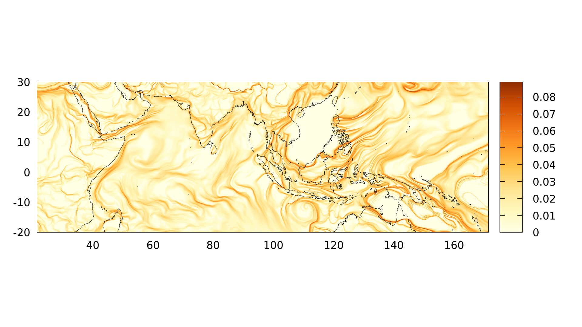
Figure 14: FTLE of ensemble member 1 and 2 of the GEFS data set.

Figure 15: GEFS ensemble with $\tau=48$ which relates to an integration time of two days. From top to bottom: D-FTLE, optimal domain displaced D-FTLE without ellipses, ellipses on FTLE values above 25% of the value range.

7.6 Performance

The computation times for the examples used in this paper are shown in table 1. $n$ denotes the number of ensembles while $\psi$ Res. and ${{\mathbf{p}}}$ Res. cover the spatial resolution of the flow and displace maps. Note, that timings for the flow map covers the time to compute for all ensembles. Same holds for ${{\mathbf{p}}}$ which shows the total compute time for all displace maps. All images shown here were computed on a 10 times higher resolution. As the computation of the optimal domain displacement is a one time preprocess which can be saved for later use, one can create higher resolution optimal domain displaced D-FTLE fields at a later time.

Flow	$n$	$\psi$ Res.	${{\mathbf{p}}}$ Res.	$\psi$ Time	${{\mathbf{p}}}$ Time
Steady DG	50	$(75,150)$	$(17,35)$	0.25 sec.	2521 sec.
Unsteady DG	50	$(75,150)$	$(17,35)$	0.25 sec.	2524 sec.
Red Sea	50	$(112,112)$	$(41,41)$	3.02 sec.	15113 sec.
Indian Sea	21	$(100,300)$	$(21,61)$	4.13 sec.	7564 sec.

Table 1: Runtime measurements for the different data sets that were used. $\psi$ Time is the time for a single iteration towards the optimal domain displacement for a single flow map. ${{\mathbf{p}}}$ Time is the summed time for all computations in order to find the optimal domain displacement for all ensemble members. This depends on the maximum iterations for the optimization which we set to 100. All measurements were taken on a Ryzen 9 3950x 16-core processor.

8 Discussion

Alternative approaches.

We propose to align flow maps. Instead, one may consider standard methods for image alignment applied to the FTLE fields of the ensemble members. Unfortunately, image-processing approaches cannot be easily applied here: they are typically based on the extraction and the alignment of point features in the image. FTLE images, however, show curved features. Therefore, the proposed flow map alignment gave more robust results than image-based FTLE alignment or alignment of the flow map gradients.

Parameters.

Our method requires some parameters: the weight $\rho$ determines the balance between alignment and rigidness (and also smoothness) for computing the domain displacements. Figure 16 shows a parameter study. In summary, we require a significant influence of the rigidity term $B$. We chose a value of $\rho=0.2$, which worked for all examples. Small variations of $\rho$ had no significant effect on the results.

Furthermore, we need to prescribe the grid defining the distortion. The number of nodes defines the degrees of freedom of the displacement function. As the displacements are expected to be smooth, this grid size can be chosen independently from the data resolution. The choice is also a balance between accurate alignment and computational cost, which increases with the degrees of freedom. We chose 30–60 nodes along the larger extent of the rectangular domains.

Note that we do not enforce bijective displacements by additional penalty terms. Figure 16 shows “flipped” cells in the deformed grid for small $\rho$, which results in a displacement mapping that cannot be inverted. This may be a rare case for our choice of $\rho$, but it is a perfectly possible case. However, our approach does not strictly require a bijective deformation of the domain. We only evaluate the “forward” deformation, but never the inverse.

3D case.

We describe our approach for 2D flows. The extension to 3D flows poses additional challenges to the general setting, the numerical optimization, performance and finally also to the visual representation. However, we do not see any fundamental issue that prevents an extension of the approach to 3D. We leave the extension to 3D for future research.

][t]0.243

][t]0.243

][t]0.243

][t]0.243

][t]0.243

][t]0.243

Figure 16: ${{\mathbf{p}}}_{1,50}$ for Double Gyre ensemble at $\tau=11$ with different weights $\rho$ for the smoothness term.
Left column from top to bottom: $\rho=0,0.2,0.4$.
Right column from top to bottom: $\rho=0.6,0.8,1$.

References

- [BT13] Barakat S. S., Tricoche X.: Adaptive refinement of the flow map using sparse samples. IEEE Trans. Vis. Comput. Graph. 19, 12 (2013), 2753–2762.
- [BWE05] Botchen R. P., Weiskopf D., Ertl T.: Texture-based visualization of uncertainty in flow fields. In IEEE Visualization (2005), pp. 647–654.
- [BWE06] Botchen R. P., Weiskopf D., Ertl T.: Interactive visualization of uncertainty in flow fields using texture-based techniques. In Electronic Proc. Intl. Symp. on Flow Visualization (2006).
- [FBW16] Ferstl F., Bürger K., Westermann R.: Streamline variability plots for characterizing the uncertainty in vector field ensembles. IEEE Transactions on Visualization and Computer Graphics 22 (2016), 767–776.
- [FH12] Farazmand M., Haller G.: Computing Lagrangian coherent structures from their variational theory. Chaos: An Interdisciplinary Journal of Nonlinear Science 22, 1 (2012), 013128.
- [GGTH07] Garth C., Gerhardt F., Tricoche X., Hagen H.: Efficient computation and visualization of coherent structures in fluid flow applications. IEEE Transactions on Visualization and Computer Graphics 13, 6 (2007).
- [GHP∗16] Guo H., He W., Peterka T., Shen H.-W., Collis S. M., Helmus J. J.: Finite-time lyapunov exponents and lagrangian coherent structures in uncertain unsteady flows. IEEE Transactions on Visualization and Computer Graphics 22, 6 (2016), 1672–1682. doi:10.1109/TVCG.2016.2534560.
- [GHS∗19] Guo H., He W., Seo S., Shen H.-W., Constantinescu E. M., Liu C., Peterka T.: Extreme-scale stochastic particle tracing for uncertain unsteady flow visualization and analysis. IEEE Transactions on Visualization and Computer Graphics 25, 9 (2019), 2710–2724. doi:10.1109/TVCG.2018.2856772.
- [GLT∗07] Garth C., Li G., Tricoche X., Hansen C., Hagen H.: Visualization of coherent structures in transient 2d flows. In Proceedings of TopoInVis (2007).
- [GOPT11] Germer T., Otto M., Peikert R., Theisel H.: Lagrangian coherent structures with guaranteed material separation. Computer Graphics Forum (Proc. EuroVis 2011) 30, 3 (2011), 761–770.
- [Hal01] Haller G.: Distinguished material surfaces and coherent structures in three-dimensional fluid flows. Physica D 149 (2001), 248–277.
- [Hal02] Haller G.: Lagrangian coherent structures from approximate velocity data. Physics of Fluids 14, 6 (2002), 1851–1861.
- [Hal15] Haller G.: Lagrangian Coherent Structures. Annual Review of Fluid Mechanics 47 (2015), 137–62.
- [HCLS16] He W., Chen C.-M., Liu X., Shen H.-W.: A bayesian approach for probabilistic streamline computation in uncertain flows. pp. 214–218. doi:10.1109/PACIFICVIS.2016.7465273.
- [HKK20] Haller G., Karrasch D., Kogelbauer F.: Barriers to the transport of diffusive scalars in compressible flows. SIAM Journal on Applied Dynamical Systems 19, 1 (2020), 85–123. doi:10.1137/19M1238666.
- [HP20] Hollister B. E., Pang A.: Uncertainty rank for streamline ensembles. Journal of Imaging Science and Technology 64(2) (2020).
- [HS11] Haller G., Sapsis T.: Lagrangian coherent structures and the smallest finite-time Lyapunov exponent. Chaos 21, 2 (2011), 023115.
- [HY00] Haller G., Yuan G.: Lagrangian coherent structures and mixing in two-dimensional turbulence. Physica D 147, 3-4 (2000).
- [LCM∗05] Lekien F., Coulliette C., Mariano A. J., Ryan E. H., Shay L. K., Haller G., Marsden J.: Pollution release tied to invariant manifolds: A case study for the coast of Florida. Physica D: Nonlinear Phenomena 210, 1-2 (2005), 1–20.
- [LM10] Lipinski D., Mohseni K.: A ridge tracking algorithm and error estimate for efficient computation of Lagrangian coherent structures. Chaos: An Interdisciplinary Journal of Nonlinear Science 20, 1 (2010).
- [MWK14] Mirzargar M., Whitaker R. T., Kirby R. M.: Curve boxplot: Generalization of boxplot for ensembles of curves. IEEE Transactions on Visualization and Computer Graphics 20 (2014), 2654–2663.
- [OGHT10] Otto M., Germer T., Hege H.-C., Theisel H.: Uncertain 2d vector field topology. In Computer Graphics Forum (Proceedings of Eurographics 2010) (Norrköping, Sweden, 5 2010).
- [OGT11] Otto M., Germer T., Theisel H.: Uncertain topology of 3d vector fields. In Proceedings of 4th IEEE Pacific Visualization Symposium (PacificVis 2011) (Hong Kong, China, March 2011), pp. 67–74.
- [PPF∗11] Pobitzer A., Peikert R., Fuchs R., Theisel H., Hauser H.: Filtering of FTLE for visualizing spatial separation in unsteady 3d flow. In Proc. TopoInVis (2011).
- [RD20] Rapp T., Dachsbacher C.: Uncertain Transport in Unsteady Flows. Tech. rep., Karlsruhe Institute of Technology, 08 2020.
- [Sci] https://kaust-vislab.github.io/SciVis2020/.
- [SFB∗12] Schindler B., Fuchs R., Barp S., Waser J., Pobitzer A., Matković K., Peikert R.: Lagrangian coherent structures for design analysis of revolving doors. IEEE Transactions on Visualization and Computer Graphics 18, 12 (2012), 2159–2168.
- [SFRS12] Schneider D., Fuhrmann J., Reich W., Scheuermann G.: A variance based ftle-like method for unsteady uncertain vector fields. In Topological Methods in Data Analysis and Visualization II: Theory, Algorithms, and Applications, Peikert R., Hauser H., Carr H., Fuchs R., (Eds.). Springer, 2012, pp. 255–268. URL: https://doi.org/10.1007/978-3-642-23175-9_17, doi:10.1007/978-3-642-23175-9_17.
- [SJK04] Sanderson A. R., Johnson C. R., Kirby R. M.: Display of vector fields using a reaction-diffusion model. In IEEE Visualization (2004), pp. 115–122.
- [SLM05a] Shadden S. C., Lekien F., Marsden J. E.: Definition and properties of Lagrangian coherent structures from finite-time Lyapunov exponents in two-dimensional aperiodic flows. Physica D 212, 7 (2005).
- [SLM05b] Shadden S. C., Lekien F., Marsden J. E.: Definition and properties of lagrangian coherent structures from finite-time lyapunov exponents in two-dimensional aperiodic flows. Physica D: Nonlinear Phenomena 212, 3 (2005), 271–304.
- [SLP∗09] Shadden S. C., Lekien F., Paduan J. D., Chavez F. P., Marsden J. E.: The correlation between surface drifters and coherent structures based on high-frequency radar data in Monterey Bay. Deep Sea Research Part II: Topical Studies in Oceanography 56, 3-5 (2009), 161 – 172.
- [SP07a] Sadlo F., Peikert R.: Efficient visualization of Lagrangian coherent structures by filtered AMR ridge extraction. IEEE Transactions on Visualization and Computer Graphics (Proc. Visualization) 13, 6 (2007).
- [SP07b] Sadlo F., Peikert R.: Visualizing Lagrangian coherent structures and comparison to vector field topology. In Proceedings of the 2007 Workshop on Topology-Based Method in Visualization (TopoInVis) (2007).
- [SPFT12] Schindler B., Peikert R., Fuchs R., Theisel H.: Ridge concepts for the visualization of Lagrangian Coherent Structures. In Topological Methods in Data Analysis and Visualization II, Peikert R., Hauser H., Carr H., Fuchs R., (Eds.), Mathematics and Visualization. Springer, 2012, pp. 221–235. URL: http://dx.doi.org/10.1007/978-3-642-23175-9_15.
- [SRP09] Sadlo F., Rigazzi A., Peikert R.: Time-Dependent Visualization of Lagrangian Coherent Structures by Grid Advection. In Topological Methods in Data Analysis and Visualization (2009), Pascucci V., Tricoche X., Hagen H., Tierny J., (Eds.), Mathematics and Visualization, Springer, pp. 151–165.
- [SW10] Sadlo F., Weiskopf D.: Time-dependent 2d vector field topology: An approach inspired by Lagrangian coherent structures. Computer Graphics Forum 29, 1 (2010), 88–100.
- [ÜSE13] Üffinger M., Sadlo F., Ertl T.: A time-dependent vector field topology based on streak surfaces. IEEE Transactions on Visualization and Computer Graphics 19, 3 (2013), 379–392.
- [WHLS18] Wang J., Hazarika S., Li C., Shen H.-W.: Visualization and visual analysis of ensemble data: A survey. IEEE Transactions on Visualization and Computer Graphics 25 (2018), 2853–2872.
- [WPJ∗08] Weldon M., Peacock T., Jacobs G. B., Helu M., Haller G.: Experimental and numerical investigation of the kinematic theory of unsteady separation. Journal of Fluid Mechanics 611 (2008).
- [ZDG∗08] Zuk T., Downton J., Gray D., Carpendale S., Liang J.: Exploration of uncertainty in bidirectional vector fields. In Society of Photo-Optical Instrumentation Engineers (SPIE) Conference Series (2008), vol. 6809, p. 68090B. published online.