Low-Complexity Control for a Class of Uncertain MIMO Nonlinear Systems under Generalized Time-Varying Output Constraints
(extended version)

Abstract

This paper introduces a novel control framework to address the satisfaction of multiple time-varying output constraints in uncertain high-order MIMO nonlinear control systems. Unlike existing methods, which often assume that the constraints are always decoupled and feasible, our approach can handle coupled time-varying constraints even in the presence of potential infeasibilities. First, it is shown that satisfying multiple constraints essentially boils down to ensuring the positivity of a scalar variable, representing the signed distance from the boundary of the time-varying output-constrained set. To achieve this, a single consolidating constraint is designed that, when satisfied, guarantees convergence to and invariance of the time-varying output-constrained set within a user-defined finite time. Next, a novel robust and low-complexity feedback controller is proposed to ensure the satisfaction of the consolidating constraint. Additionally, we provide a mechanism for online modification of the consolidating constraint to find a least violating solution when the constraints become mutually infeasible for some time. Finally, simulation examples of trajectory and region tracking for a mobile robot validate the proposed approach.

I Introduction

In the last decade, the control of nonlinear systems under constraints has gained significant interest, driven by both practical necessities and challenging theoretical aspects. Constraints play a pervasive role in the design of controllers for practical nonlinear systems, often representing critical performance and safety requirements. Their violation can lead to performance deterioration, system damage, and potential hazards. Over the years, a variety of approaches have emerged to address different types of constraints within control systems, such as model predictive control, reference governors, control barrier functions, funnel control, prescribed performance control, and barrier Lyapunov functions as documented in [1, 2, 3, 4, 5, 6, 7, 8, 9].

This work focuses on (closed-form) feedback control designs under time-varying output constraints, a crucial area in nonlinear control systems driven by the need to ensure tracking and stabilization performance as well as safety requirements [5, 6, 10, 9, 8, 11]. Existing closed-form feedback control approaches for addressing time-varying output constraints fall into three primary categories: Funnel Control (FC) [6, 7], Prescribed Performance Control (PPC) [8, 9], and Time-Varying Barrier Lyapunov Function (TVBLF) methods [5]. Typically, control designs based on FC, PPC, and TVBLF are commonly employed to achieve user-defined transient and steady-state performance for tracking and stabilization errors. These designs restrict errors evolution within user-defined time-varying funnels, serving as the sole output constraints. For example, in these studies, constraints of the form $-\rho_{i}(t)<e_{i}=x_{i}-x_{i}^{d}(t)<\rho_{i}(t)$ are frequently used for independent tracking errors, where $x_{i}$ represents independent state variables, $x_{i}^{d}(t)$ denotes desired trajectories, and $\rho_{i}(t)$ signifies bounded, strictly positive time-varying functions that model the evolving behavior of these constraints. To ensure the desired transient and steady-state performance of tracking errors, $\rho_{i}(t)$ is often selected as a strictly positive exponentially decaying function, approaching a small neighborhood of zero [8, 6].

In recent years, significant advancements have emerged in the utilization of FC, PPC, and TVBLF methods. These developments encompass a broad spectrum of applications, including the control of high-order systems [9, 11, 12, 10, 13], output feedback [14, 15], multi-agent systems [16, 17, 18, 19, 20, 21, 22, 23, 24, 25]. Additionally, there are works addressing considerations such as unknown control directions [26, 27, 28], control input constraints [29, 30, 31, 32, 33, 34, 35], actuator faults [36, 37], discontinuous output tracking [38], event-triggered control [39], asymptotic tracking [40, 41, 42, 43], and signal temporal logic specifications [44, 45, 46, 47], among others. Furthermore, researchers dedicated efforts to crafting specific designs for time-varying boundary functions of funnel constraints to guarantee finite/fixed time (practical) tracking and stabilization [48, 49], considering asymmetric funnel constraints [50], introducing monotone tube boundaries to enhance control precision [51], and addressing compatibility between output and state constraints [52]. In the same direction, works on hard and soft constraints [53] and reach-avoid specifications [54] have also been conducted. For recent surveys on FC and PPC see [55, 56].

While FC, PPC, and TVBLF approaches have demonstrated success in various applications and developments, they still face limitations when it comes to handling couplings between multiple time-varying constraints. These methods primarily focus on time-varying funnel constraints applied to independent states or error signals, which inherently remain decoupled from each other. In other words, these methods implicitly assume that the satisfaction of one funnel constraint does not impact the satisfaction of the others. To be more precise, the funnel constraints considered in FC, PPC, and TVBLF methods can be liked to time-varying box constraints in the system’s output or error space [10, 9, 50]. In addition, it is also known that these methods are restricted to systems with the same number of inputs and outputs. However, in various practical applications, such as those involving general safety considerations [57] and general spatiotemporal specifications [44], there is a need to address arbitrary and potentially coupled multiple time-varying output constraints. Consequently, it becomes crucial to develop control methodologies for uncertain nonlinear systems that can handle a more general class of time-varying output constraints. Recently, [53] proposed a low-complexity feedback control law under both hard and soft funnel constraints. Nevertheless, even when there are couplings between these hard and soft funnel constraints, the approach in [53] treats all hard constraints as independent funnels, adhering to the established conventions. In addition, inspired by [53], authors in [54] introduced a funnel-based control for handling reach-avoid specifications by carefully designing funnel boundaries. However, once again, this work does not directly address the consideration of couplings between multiple time-varying output constraints.

In this paper, we present a novel feedback control law that aims at satisfying potentially coupled, time-varying output constraints for uncertain high-order MIMO nonlinear systems. Drawing inspiration from the approach introduced in [44], our control design revolves around consolidating all time-varying constraints into a carefully crafted single constraint. To ensure the satisfaction of this consolidating constraint, we introduce a new low-complexity robust control strategy inspired by [9]. Notably, the approach does not rely on approximations or parameter estimation schemes to handle system uncertainties. Additionally, we demonstrate that by adaptively adjusting the consolidating constraint online, we can achieve a least violating solution for the closed-loop system when the constraints become infeasible during an unknown time interval.

In contrast to existing FC, PPC, TVBLF methods, which primarily impose symmetric funnel constraints on system outputs, our approach not only encompasses generic asymmetric funnel constraints but also one-sided (time-varying) constraints on system outputs, which allows for taking into consideration more general type of spatiotemporal specifications. Moreover, while the aforementioned control methods require the fulfillment of all output constraints at the initial time, our method allows for achieving convergence to the time-varying output-constrained set within a user-defined finite time, even when the constraints are not initially met. More precisely, the proposed control method guarantees convergence to and invariance of the time-varying output-constrained set within an appointed finite time. Overall, our results extend the scope of feedback control designs for nonlinear systems, accommodating a broader range of time-varying output constraints. Notably, closed-form feedback control designs for reference tracking under a prescribed performance and handling time-invariant output constraints in nonlinear systems fit into our results as special cases.

In connection with our methodology presented in this paper, related works in [57, 58, 59] share a common approach of constructing a single time-invariant Control Barrier Function (CBF) to satisfy multiple time-invariant constraints. It is worth noting that time-varying CBFs can also be employed for controlling nonlinear systems under time-varying output constraints, as studied in [60, 61, 62]. However, traditional control synthesis using the CBF concept typically necessitates precise knowledge of the system dynamics and involves solving an online Quadratic Programming problem, which may not be favorable in certain applications. In contrast, our work offers a computationally tractable (optimization-free) and robust (model-free) feedback control law.

The preliminary findings of this study were outlined in [63], focusing exclusively on first-order nonlinear MIMO systems with a time-invariant output map. This paper builds upon the foundation laid in [63], extending our research to encompass high-order nonlinear MIMO systems with a time-varying output map. This expansion broadens the range of time-varying constraints that our method can effectively handle. Notably, in contrast to the single funnel constraint employed in [63], we utilize a one-sided consolidating constraint in this work, which further simplifies the controller design and tuning process. Additionally, this paper addresses the challenge of potential constraint infeasibilities, a consideration not addressed in [63].

Notations: $\mathbb{R}^{n}$ is the real $n$-dimensional space and $\mathbb{N}$ is the set of natural numbers. $\mathbb{R}_{\geq 0}$ and $\mathbb{R}_{>0}$ represent non-negative and positive real numbers. A vector $x\in\mathbb{R}^{n}$ is an $n\times 1$ column vector, and $x^{\top}$ is its transpose. The Euclidean norm of $x$ is $\|x\|$. The concatenation operator is $\mathrm{col}(x_{i})\coloneqq[x_{1}^{\top},\ldots,x_{m}^{\top}]^{\top}\in\mathbb{R}^{mn}$, where $x_{i}\in\mathbb{R}^{n},i=\{1,\ldots,m\}$. The space of real $n\times m$ matrices is $\mathbb{R}^{n\times m}$. For a matrix $A\in\mathbb{R}^{n\times m}$, $A^{\top}$ is the transpose, $\lambda_{\textit{min}}(A)$ is the minimum eigenvalue, and $\|A\|$ is the induced matrix norm. The operator $\mathrm{diag}(\cdot)$ constructs a diagonal matrix from its arguments. The absolute value of a real number is $|\cdot|$. For a set $\Omega$, $\partial\Omega$ is the boundary, and $\mathrm{cl}(\Omega)$ is the closure. $\otimes$ represents the Kronecker product and $\mathbf{0}_{n}\in\mathbb{R}^{n}$ is the vector of zeros. The set of $n$-times continuously differentiable functions is $\mathcal{C}^{n}$. The index set notation is $\mathcal{I}_{i}^{j}=\{i,\ldots,j\}$, where $i,j\in\mathbb{N}$ and $i<j$.

II Problem Formulation

Consider a class of general high-order MIMO nonlinear systems described by the following dynamics:

$$\!\!\!\!\!\!\!\!\begin{cases}\dot{x}_{i}=f_{i}(t,\bar{x}_{i})+G_{i}(t,\bar{x}_{i})x_{i+1}+w_{i}(t),\;i\in\mathcal{I}_{1}^{r-1},\\ \dot{x}_{r}=f_{r}(t,\bar{x}_{r})+G_{r}(t,\bar{x}_{r})u+w_{r}(t),\\ y=h(t,x_{1}),\end{cases}\!\!\!\!\!\!\!\!\!\!\!\!\!\!\!\!\!\!\!$$ (1)

where $x_{i}\coloneqq[x_{i,1},x_{i,2},\ldots,x_{i,n}]^{\top}\in\mathbb{R}^{n}$, $\bar{x}_{i}\coloneqq[x_{1}^{\top},\ldots,x_{i}^{\top}]^{\top}\in\mathbb{R}^{ni},i\in\mathcal{I}_{1}^{r}$, $r\in\mathbb{N}$, and $x\coloneqq\bar{x}_{r}\in\mathbb{R}^{nr}$ is the state vector. Moreover, $u\in\mathbb{R}^{n}$ and $y=[y_{1},y_{2},\ldots,y_{m}]^{\top}\in\mathbb{R}^{m}$ denote the control input and output vectors, respectively, and $w_{i}:\mathbb{R}_{\geq 0}\rightarrow\mathbb{R}^{n},i\in\mathcal{I}_{1}^{r}$ represent external disturbance vectors. In addition, $f_{i}:\mathbb{R}_{\geq 0}\times\mathbb{R}^{ni}\rightarrow\mathbb{R}^{n},i\in\mathcal{I}_{1}^{r}$ denote the vectors of nonlinear functions that are locally Lipschitz in $\bar{x}_{i}$ and piece-wise continuous in $t$. Moreover, $G_{i}:\mathbb{R}_{\geq 0}\times\mathbb{R}^{ni}\rightarrow\mathbb{R}^{n\times n},i\in\mathcal{I}_{1}^{r}$ stand for the control coefficient matrices whose elements are locally Lipschitz in $\bar{x}_{i}$ and piece-wise continuous in $t$. Finally, $h:\mathbb{R}_{\geq 0}\times\mathbb{R}^{n}\rightarrow\mathbb{R}^{m}$ is a $\mathcal{C}^{2}$ map in $x_{1}$ and $\mathcal{C}^{1}$ in $t$. In particular, let $h(t,x_{1})=[h_{1}(t,x_{1}),h_{2}(t,x_{1}),\ldots,h_{m}(t,x_{1})]^{\top}$, so that $y_{i}=h_{i}(t,x_{1}),i\in\mathcal{I}_{1}^{m}$. Let $x(t;x(0),u)$ denote the solution of the closed-loop system (1) under the control law $u$ and the initial condition $x(0)$. For brevity in the notation, from now on we will use $x(t;x(0))$ instead of $x(t;x(0),u)$. Moreover, consider $x_{1}(t;x(0))$ as the partial solution of the closed-loop system (1) with respect to states $x_{1}$ under the initial condition $x(0)$ and the control input $u$.

In this paper, we pose the following technical assumptions for (1). Note that these assumptions do not restrict the applicability of our results, as they are relevant to the high-order practical mechanical systems under consideration.

Assumption 1

The functions $f_{i}(t,\bar{x}_{i}),i\in\mathcal{I}_{1}^{r}$, are unknown and there exist locally Lipschitz functions $\bar{f}_{i}:\mathbb{R}^{ni}\rightarrow\mathbb{R}^{n},i\in\mathcal{I}_{1}^{r}$, with unknown analytical expressions such that $\|f_{i}(t,\bar{x}_{i})\|\leq\|\bar{f}_{i}(\bar{x}_{i})\|$, for all $t\geq 0$, and all $\bar{x}_{i}\in\mathbb{R}^{ni}$.

Assumption 2

The matrices $G_{i}(t,\bar{x}_{i}),i\in\mathcal{I}_{1}^{r}$ are unknown and (A) there exist locally Lipschitz functions $\bar{g}_{i}:\mathbb{R}^{ni}\rightarrow\mathbb{R},i\in\mathcal{I}_{1}^{r}$, with an unknown analytical expression such that $\|G_{i}(t,\bar{x}_{i})\|\leq\bar{g}_{i}(\bar{x}_{i})$, $\forall t\geq 0$; (B) the symmetric components denoted by $G_{i}^{s}(t,\bar{x}_{i})\coloneqq\frac{1}{2}\left(G_{i}^{\top}(t,\bar{x}_{i})+G_{i}(t,\bar{x}_{i})\right),i\in\mathcal{I}_{1}^{r}$, are uniformly sign-definite with known signs. Without loss of generality, we assume that all $G_{i}^{s}(t,\bar{x}_{i})$ are uniformly positive definite, i.e., $z^{\top}G_{i}^{s}(t,\bar{x}_{i})z>0,\forall t\in\mathbb{R}_{\geq 0},\forall z\in\mathbb{R}^{n}$, and $\forall\bar{x}_{i}\in\mathbb{R}^{ni}$, with $z\neq\mathbf{0}_{n}$.

Assumption 3

The functions $w_{i}(t),i\in\mathcal{I}_{1}^{r}$ are unknown, bounded and piece-wise continuous, with $\|w_{i}(t)\|\leq\bar{w}_{i},\forall t\geq 0,i\in\mathcal{I}_{1}^{r}$, in which the constant upper bounds $\bar{w}_{i}$ are unknown.

Part (B) of Assumption 2 establishes a global controllability condition for (1). It implies the existence of strictly positive constants $\underline{\lambda}_{i}>0,i\in\mathcal{I}_{1}^{r}$, such that $\lambda_{\textit{min}}(G_{i}^{s}(t,\bar{x}_{i}))\geq\underline{\lambda}_{i}>0$, for all $\bar{x}_{i}\in\mathbb{R}^{ni}$ and all $t\geq 0$. Furthermore, Assumptions 1 and 2 suggest that while the elements of $f_{i}(t,\bar{x}_{i})$ and $G_{i}(t,\bar{x}_{i})$, $i\in\mathcal{I}_{1}^{r}$, can grow arbitrarily large due to variations in $\bar{x}_{i}$, they cannot do so as a result of increase in $t$. The following assumptions solely pertain to the output map of (1).

Assumption 4

There exists a continuous function $\kappa_{0}:\mathbb{R}^{n}\rightarrow\mathbb{R}$, such that $\|J(t,x_{1})\|\leq\kappa_{0}(x_{1})$, where $J(t,x_{1})\coloneqq\frac{\partial h(t,x_{1})}{\partial x_{1}}$ is the Jacobian of the output map.

Assumption 5

There exist continuous functions $\kappa_{i},\bar{h}_{i}:\mathbb{R}^{n}\rightarrow\mathbb{R},i\in\mathcal{I}_{1}^{m}$, such that $|h_{i}(t,x_{1})|\leq\bar{h}_{i}(x_{1})$ and $|\frac{\partial h_{i}(t,x_{1})}{\partial t}|\leq\kappa_{i}(x_{1})$, respectively.

Assumptions 4 and 5 ensure that the elements of the Jacobian matrix $J(t,x_{1})$ and the functions $h_{i}(t,x_{1})$ and $\frac{\partial h_{i}(t,x_{1})}{\partial t}$, $i\in\mathcal{I}_{1}^{m}$, can grow arbitrarily large only as a result of changes in $x_{1}$, and not due to increase in $t$.

Remark 1

Assumptions 4 and 5 can be omitted if $h(t,x_{1})$ in (1) does not explicitly depend on time, i.e., $h(x_{1})$, with $h(x_{1})$ only requiring to be a $\mathcal{C}^{2}$ function. Additionally, if $f_{i}(t,\bar{x}_{i})$ and $G_{i}(t,\bar{x}_{i}),i\in\mathcal{I}_{1}^{r}$ in (1), are replaced by $f_{i}(\bar{x}_{i})$ and $G_{i}(\bar{x}_{i})$, then Assumptions 1 and 2 simplify to standard requirements. These requirements then only necessitate $f_{i}$ and $G_{i}$ to be locally Lipschitz and $G_{i}^{s}(\bar{x}_{i})=\frac{1}{2}\left(G_{i}^{\top}(\bar{x}_{i})+G_{i}(\bar{x}_{i})\right)$ to be positive definite for all $\bar{x}_{i}\in\mathbb{R}^{ni}$.

Let the outputs of (1) be subject to the following class of time-varying constraints:

$$\!\!\!\underline{\rho}_{i}(t)<h_{i}(t,x_{1})<\overline{\rho}_{i}(t),\;\;i\in\mathcal{I}_{1}^{m},\;\;\forall t\geq 0,\!$$ (2)

where $\underline{\rho}_{i},\overline{\rho}_{i}:\mathbb{R}_{\geq 0}\rightarrow\mathbb{R}\cup\{\pm\infty\},i\in\mathcal{I}_{1}^{m}$. We assume for each $i\in\mathcal{I}_{1}^{m}$, that at least one of $\overline{\rho}_{i}(t)$ and $\underline{\rho}_{i}(t)$ is a bounded $\mathcal{C}^{1}$ function of time with a bounded derivative. In other words, we allow $\underline{\rho}_{i}(t)=-\infty$ (resp. $\overline{\rho}_{i}(t)=+\infty$) when $\overline{\rho}_{i}(t)$ (resp. $\underline{\rho}_{i}(t)$) is bounded for all $t\geq 0$. In this respect, (2) can either represent Lower Bounded One-sided (LBO) time-varying constraints in the form of $\underline{\rho}_{i}(t)<h_{i}(t,x_{1})$, Upper Bounded One-sided (UBO) time-varying constraints in the form of $h_{i}(t,x_{1})<\overline{\rho}_{i}(t)$, as well as (time-varying) funnel constraints in the form of $\underline{\rho}_{i}(t)<h_{i}(t,x_{1})<\overline{\rho}_{i}(t)$, for which both $\overline{\rho}_{i}(t)$ and $\underline{\rho}_{i}(t)$ are bounded.

Without loss of generality, we assume that the first $p$ constraints in (2), i.e., for $i\in\mathcal{I}_{1}^{p},0\leq p\leq m$, are funnel constraints, $q$ LBO constraints are indexed by $i\in\mathcal{I}_{p+1}^{p+q},0\leq q\leq m-p$ in (2), and the remaining $m-p-q$ constraints represent UBO constraints for which $i\in\mathcal{I}_{p+q+1}^{m}$ in (2). We make the assumption that each funnel constraint in (2) is well-defined, i.e., for every $i\in\mathcal{I}_{1}^{p}$, there exists a positive constant $\epsilon_{i}$ such that $\overline{\rho}_{i}(t)-\underline{\rho}_{i}(t)\geq\epsilon_{i},\forall t\geq 0$. This condition guarantees that the $p$ funnel constraints are independently feasible.

Remark 2

Note that the output constraints specified in (2) depend on $x_{1}$, which signifies the spatial coordinates (positions) of mechanical systems. Furthermore, while previous works particularly only deal with $n$ decoupled funnel constraints by considering $y=x_{1}$, we account for $m\geq n$ generalized system outputs denoted as $y=h(t,x_{1})$ in (1), which allows for possible couplings between different constraints presented in (2).

We emphasize that, in this paper, the output map $h(t,x_{1})$ is primarily employed to incorporate various types of constraints into the nonlinear dynamics described by (1). Specifically, we utilize $h(t,x_{1})$ in conjunction with the time-varying functions $\underline{\rho}_{i}(t)$ and $\overline{\rho}_{i}(t)$ in (2) to represent various forms of spatiotemporal constraints for (1). Note that, $h(t,x_{1})$ is not necessarily related to the available measurements of the system. As we will further elaborate, we assume that the states of (1) are available for the measurement and will be utilized for designing the control input $u(t,x)$.

Definition 1

An output of (1), $y_{i}=h_{i}(t,x_{1})$, is called separable if it can be expressed as the sum of a component solely varying with time and another component dependent solely on $x_{1}$, i.e., $h_{i}(t,x_{1})=h_{i}^{x_{1}}(x_{1})+h_{i}^{t}(t)$. Otherwise, it is called inseparable.

Note that, if $y_{i}=h_{i}(t,x_{1})$ is separable, the time-varying term $h_{i}^{t}(t)$ can be incorporated into the time-varying bounds $\overline{\rho}_{i}(t)$ and $\underline{\rho}_{i}(t)$ in (2). Thus, one can consider the time-independent output $h_{i}^{x_{1}}(x_{1})$ instead of $h_{i}(t,x_{1})$ in (1). For example, let (1) model a moving vehicle with position $[x_{1,1},x_{1,2}]^{\top}$, and the objective is to track a $\mathcal{C}^{1}$ reference trajectory characterized by $x_{1}^{d}(t)=[x_{1,1}^{d}(t),x_{1,2}^{d}(t)]^{\top}$ under the funnel constraints $-\rho_{i}(t)<h_{i}(t,x_{1})=x_{1,i}-x_{1,i}^{d}(t)<\rho_{i}(t),i\in\mathcal{I}_{1}^{2}$, where $\rho_{i}(t)$ are positive functions decaying to a small neighborhood of zero (tracking under a prescribed performance, see [8]). Here $h_{i}(t,x_{1}),i\in\mathcal{I}_{1}^{2}$ represent the tracking errors and the constraints can be written as $x_{1,i}^{d}(t)-\rho_{i}(t)<x_{1,i}<\rho_{i}(t)+x_{1,i}^{d}(t),i\in\mathcal{I}_{1}^{2}$. On the other hand, if the vehicle is tasked with reaching a moving target defined by its position $x_{1}^{d}(t)$, then a single constraint can be imposed: $-\rho(t)<h(t,x_{1})=(x_{1,1}-x_{1,1}^{d}(t))^{2}+(x_{1,2}-x_{1,2}^{d}(t))^{2}<\rho(t)$, where $\rho(t)$ is a positive function decaying to a neighborhood of zero and $h(t,x_{1})$ represents the squared distance error, which has inseparable time-varying terms.

Finally, let us define the output constrained set $\bar{\Omega}(t)$ based on (2) as:

$$\bar{\Omega}(t)\coloneqq\{x_{1}\in\mathbb{R}^{n}\mid\underline{\rho}_{i}(t)<h_{i}(t,x_{1})<\overline{\rho}_{i}(t),i\in\mathcal{I}_{1}^{m}\}.$$ (3)

Objective: In this paper, our goal is to design a low-complexity continuous robust feedback control law $u(t,x)$ for (1) such that $x_{1}(t;x(0))$ satisfies the time-varying output constraints (2) $\forall t>T\geq 0$, where $T$ is a user-defined finite time after which the output constraints are satisfied for all time (i.e., $x_{1}(t;x(0))\in\bar{\Omega}(t),\forall t>T\geq 0$). Note that this problem reduces to establishing only invariance of $\bar{\Omega}(t)$ for all $t\geq 0$, if $x_{1}(0)\in\bar{\Omega}(0)$ ($T=0$). On the other hand, having $x_{1}(0)\notin\bar{\Omega}(0)$ indicates establishing: (i) finite time convergence to $\bar{\Omega}(t)$ at $t=T$, and (ii) ensuring invariance of $\bar{\Omega}(t)$, for all $t>T$. Furthermore, when $\bar{\Omega}(t)$ becomes infeasible (empty) for an unknown time interval, we aim at enhancing the control scheme such that $u(t,x)$ drives the closed-loop system trajectory towards a least violating solution for (1) under (2) (see Section IV for more details).

III Main Results

In this section, inspired from [44], we first introduce a novel scalar variable, which is the signed distance from the boundary of the time-varying output constrained set (3). This variable serves as a metric of both feasibility and satisfaction of the output constraints. Next, we propose a robust and low-complexity controller design for (1), which ensures the ultimate positivity of the aforementioned variable. This, in turn, leads to the satisfaction of the output constraints.

III-A Satisfying Constraints using a Scalar Variable

Notice that the $m$ output constraints in (2) can be re-written in the following format:

(4a)

(4b)

Now, without loss of generality, consider all these $m+p$ constraints in (4) as:

$$\psi_{i}(t,x_{1})>0,\quad i\in\mathcal{I}_{1}^{m+p},$$ (5)

where $\psi_{i}:\mathbb{R}_{\geq 0}\times\mathbb{R}^{n}\rightarrow\mathbb{R}$ are $\mathcal{C}^{2}$ in $x_{1}$ and $\mathcal{C}^{1}$ in $t$. As a result, one can re-write (3) as:

$$\bar{\Omega}(t)=\{x_{1}\in\mathbb{R}^{n}\mid\psi_{i}(t,x_{1})>0,\forall i\in\mathcal{I}_{1}^{m+p}\}.$$ (6)

Now let us define the scalar function $\bar{\alpha}:\mathbb{R}_{\geq 0}\times\mathbb{R}^{n}\rightarrow\mathbb{R}$, as:

$$\bar{\alpha}(t,x_{1})\coloneqq\min\{\psi_{1}(t,x_{1}),\ldots,\psi_{m+p}(t,x_{1})\},$$ (7)

where $\bar{\alpha}(t,x_{1})$ represents the signed (minimum) distance from $\partial\mathrm{cl}(\bar{\Omega}(t))$. In this respect, one can re-write (6) as the zero super level set of $\bar{\alpha}(t,x_{1})$:

$$\bar{\Omega}(t)=\{x_{1}\in\mathbb{R}^{n}\mid\bar{\alpha}(t,x_{1})>0\}.$$ (8)

Note that if $\bar{\alpha}(t^{\prime},x_{1})<0$, then at least one constraint is not satisfied at $t=t^{\prime}$, while $\bar{\alpha}(t,x_{1})>0,\forall t\geq 0$ means that all constraints are satisfied for all time. Owing to the $\min$ operator in (7), in general, $\bar{\alpha}(t,x_{1})$ is a continuous but nonsmooth function, therefore, to facilitate the controller design and stability analysis we will consider the smooth under-approximation of $\bar{\alpha}(t,x_{1})$ given by the following log-sum-exp function [64]:

$$\alpha(t,x_{1}) \coloneqq-\frac{1}{\nu}\ln\Big{(}\sum_{i=1}^{m+p}e^{-\nu\,\psi_{i}(t,x_{1})}\Big{)}$$ (9a)

$$\leq\bar{\alpha}(t,x_{1})\leq\alpha(t,x_{1})+\frac{1}{\nu}\ln(m+p),$$ (9b)

where $\nu>0$ is a tuning coefficient whose larger values gives a closer (under) approximation (i.e, $\alpha(t,x_{1})\rightarrow\bar{\alpha}(t,x_{1})$ as $\nu\rightarrow\infty$). Note that, $\alpha(t,x_{1})$ provides the signed distance from the boundary of a smooth inner-approximation of $\mathrm{cl}(\bar{\Omega}(t))$. Therefore, ensuring $\alpha(t,x_{1})>0,\forall t\geq 0$ guarantees $\bar{\alpha}(t,x_{1})>0,\forall t\geq 0$ and thus the satisfaction of (5) (equivalently (2)). Define $\Omega(t)\subset\bar{\Omega}(t)$ as the smooth inner-approximation of the set $\bar{\Omega}(t)$, given by:

$$\Omega(t)\coloneqq\{x_{1}\in\mathbb{R}^{n}\mid\alpha(t,x_{1})>0\}.$$ (10)

Note that we have $x_{1}\in\Omega(t)\Rightarrow x_{1}\in\bar{\Omega}(t)$, and when $\bar{\Omega}(t)$ is bounded, then $\Omega(t)$ is also bounded. Fig. 1 depicts snapshots of $\bar{\Omega}(t)$ and $\Omega(t)$ with $\nu=2$ in (9) for the following examples:

Example 1

Consider $h(x_{1})=[h_{1}(x_{1}),h_{2}(x_{1}),h_{3}(x_{1})]^{\top}$, where $h_{1}(x_{1})=x_{1,1}$, $h_{2}(x_{1})=-x_{1,1}+x_{1,2}$, and $h_{3}(x_{1})=0.3x_{1,1}^{2}+x_{1,2}$ and let the output constraints be $\underline{\rho}_{1}(t)<h_{1}(x_{1})<\overline{\rho}_{1}(t)$ (funnel constraint), $\underline{\rho}_{2}(t)<h_{2}(x_{1})$ (LBO constraint), and $h_{3}(x_{1})<\overline{\rho}_{3}(t)$ (UBO constraint), respectively. Fig. 1(a) depicts a snapshot of the time-varying output constrained set and its smooth inner approximation, for which $-\underline{\rho}_{1}(t)=\overline{\rho}_{1}(t)=2$, $\underline{\rho}_{2}(t)=-2$, and $\overline{\rho}_{3}(t)=4$.

Example 2

Consider $h(x_{1})=[h_{1}(x_{1}),h_{2}(x_{1})]^{\top}$, with $h_{1}(x_{1})=x_{1,1}$ and $h_{2}(x_{1})=0.3x_{1,1}^{2}-x_{1,2}$ and let the output constraints be $\underline{\rho}_{1}(t)<h_{1}(x_{1})<\overline{\rho}_{1}(t)$ and $\underline{\rho}_{2}(t)<h_{2}(x_{1})<\overline{\rho}_{2}(t)$ (two funnel constraints), respectively. Fig. 1(b) depicts a snapshot of the time-varying output-constrained set and its smooth inner-approximation, for which $\underline{\rho}_{1}(t)=-3,\overline{\rho}_{1}(t)=2$, and $-\underline{\rho}_{2}(t)=\overline{\rho}_{2}(t)=2$.

Example 3

Consider the constraints of Example 2, however, this time we modify the second output such that $h_{2}(t,x_{1})=c_{1}(t)(x_{1,1}-o_{1}(t))^{2}-x_{1,2}$, where $c_{1}(t)$ and $o_{1}(t)$ are bounded continuously differentiable time-varying functions. Fig. 1(c) depicts three snapshots of the time-varying output-constrained set and its smooth inner-approximations, for which $\underline{\rho}_{1}(t_{1})=-3,\overline{\rho}_{1}(t_{1})=2,\underline{\rho}_{1}(t_{2})=4,\overline{\rho}_{1}(t_{2})=9,\underline{\rho}_{1}(t_{3})=11,\overline{\rho}_{1}(t_{3})=16$, and $-\underline{\rho}_{2}(t)=\overline{\rho}_{2}(t)=2,\forall t\in\{t_{1},t_{2},t_{3}\}$, where $t_{1}<t_{2}<t_{3}$. Moreover, $c_{1}(t_{1})=0.3,c_{1}(t_{2})=0,c_{1}(t_{3})=-0.3$ and $o_{1}(t_{1})=0,o_{1}(t_{2})=6,o_{1}(t_{3})=13$. Note that different from Example 2, $o_{1}(t)$ and $c_{1}(t)$ in $h_{2}(t,x_{1})$ can contribute in shifting and changing the boundaries of the time-varying constrained set simultaneously at different time instances.

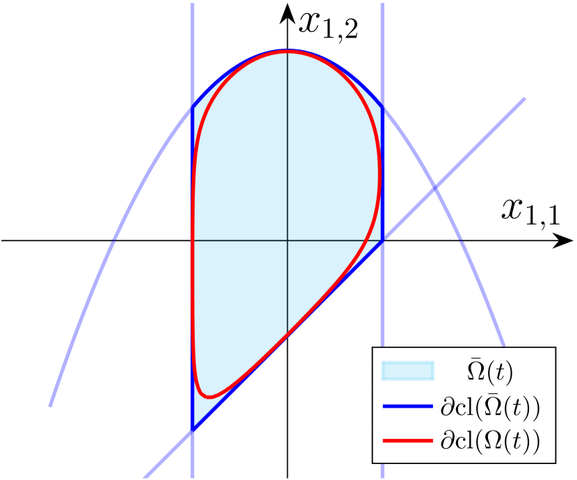
(a)

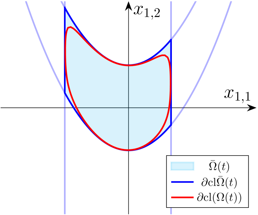
(b)

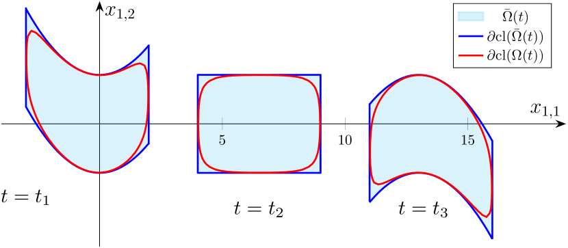
(c)

Figure 1: Snapshots of $\bar{\Omega}(t)$ and its corresponding inner-approximation under (9) for three different examples.

Assumption 6

The function $-\bar{\alpha}(t,x_{1})$ is coercive (radially unbounded) in $x_{1}$ and uniformly in $t$, i.e, $-\bar{\alpha}(t,x_{1})\rightarrow+\infty$ as $\|x_{1}\|\rightarrow+\infty,\forall t\geq 0$.

Note that, the focus of this work is the satisfaction of (2). On the other hand, it is also essential to design $u(t,x)$ such that $\|x_{i}(t)\|,i=\mathcal{I}_{1}^{r}$ remain bounded $\forall t\geq 0$. In this respect, if the output-constrained set $\bar{\Omega}(t)$ is well-posed (i.e, it is bounded), the satisfaction of the constraints inherently leads to the boundedness of $\|x_{1}(t)\|$. Assumption 6 serves as a necessary and sufficient condition for ensuring the boundedness of $\bar{\Omega}(t)$ (and $\Omega(t)$) for all $t\geq 0$. The following lemma establishes this.

Lemma 1

Under Assumption 6, $\bar{\Omega}(t)$ (resp. $\Omega(t)$) is a bounded set for all $t\geq 0$.

Proof:

See Appendix A. ∎

Note that, Assumption 6 implies that for any time instant $-\bar{\alpha}(t,x_{1})$ should approach $+\infty$ along any path within $\mathbb{R}^{n}$ on which $\|x_{1}\|$ tends to infinity. Define $h_{f}(t,x_{1})\coloneqq\mathrm{col}(h_{i}(t,x_{1}))\in\mathbb{R}^{p},i\in\mathcal{I}_{1}^{p}$, $h_{\mathrm{L}}(t,x_{1})\coloneqq\mathrm{col}(h_{i}(t,x_{1}))\in\mathbb{R}^{q},i\in\mathcal{I}_{p+1}^{p+q}$, and $h_{\mathrm{U}}(t,x_{1})\coloneqq\mathrm{col}(h_{i}(t,x_{1}))\in\mathbb{R}^{m-p-q},i\in\mathcal{I}_{p+q+1}^{m}$, as the stacked vectors of system outputs associated with funnel, LBO, and UBO constraints in (2), respectively. The following lemma provides explicit conditions on $h_{i}(t,x_{1}),i\in\mathcal{I}_{1}^{m}$, to ensure that $-\bar{\alpha}(t,x_{1})$ (resp. $-\alpha(t,x_{1})$) is coercive.

Lemma 2

The function $-\bar{\alpha}(t,x_{1})$ (resp. $-\alpha(t,x_{1})$) is coercive in $x_{1}$ for all $t\geq 0$ if and only if, for each time instant $t$, at least one of the following conditions holds:

• $\|h_{f}(t,x_{1})\|\rightarrow+\infty$;

• one or more elements of $h_{\mathrm{L}}(t,x_{1})$ approaches $-\infty$;

• one or more elements of $h_{\mathrm{U}}(t,x_{1})$ approaches $+\infty$;

along any path in $\mathbb{R}^{n}$ as $\|x_{1}\|\rightarrow+\infty$.

Proof:

See Appendix B. ∎

In Example 1, we observe that $h_{f}(t,x_{1})=h_{1}(x_{1})$, $h_{L}(t,x_{1})=h_{2}(x_{1})$, $h_{U}(t,x_{1})=h_{3}(x_{1})$. It can be verified that the condition in Lemma 2 is satisfied along any path in $\mathbb{R}^{2}$ as $\|x_{1}\|\rightarrow+\infty$. Hence, $-\bar{\alpha}(t,x_{1})$ (resp. $-\alpha(t,x_{1})$) is coercive, implying that $\bar{\Omega}(t)$ (resp. $\Omega(t)$) is bounded based on Lemma 1 (See Fig. 1(a)). However, if we remove the LBO constraint $\underline{\rho}_{2}(t)<h_{2}(x_{1})=x_{1,2}-x_{1,1}$, $\bar{\Omega}(t)$ (and $\Omega(t)$) will not be bounded since along the path where $x_{1,1}=0$ and $x_{1,2}\rightarrow-\infty$ we get $h_{f}(x_{1})=0$, $h_{U}(x_{1})\rightarrow-\infty$, which do not satisfy any of the conditions in Lemma 2. In Example 2, we have $h_{f}(t,x_{1})=[h_{1}(x_{1}),h_{2}(x_{1})]^{\top}$. One can verify that $\|h_{f}(t,x_{1})\|\rightarrow+\infty$ along any path in $\mathbb{R}^{2}$ as $\|x_{1}\|\rightarrow+\infty$. In Example 3, we observe that $h_{f}(t,x_{1})=[h_{1}(x_{1}),h_{2}(t,x_{1})]^{\top}$. It is not difficult to see that Condition I in Lemma 2 holds for all time instances and as depicted in Fig. 1(c), $\bar{\Omega}(t)$ (resp. $\Omega(t)$) remains bounded $\forall t\geq 0$.

Verifying the boundedness of $\bar{\Omega}(t)$ as per Lemma 1 can be challenging, especially when dealing with time-dependent outputs (i.e., $h_{i}(t,x_{1})$ instead of $h_{i}(x_{1})$). In such cases, one must check the condition in Lemma 2 for all time instances. However, note that ensuring the boundedness of $\bar{\Omega}(t)$ is merely a technical requirement in this paper. To meet this requirement, one approach is to introduce an auxiliary output, denoted as $h_{\mathrm{aux}}(x_{1})$, under the UBO constraint: $h_{\mathrm{aux}}(x_{1})\coloneqq\|x_{1}\|<c_{\mathrm{aux}}$, where $c_{\mathrm{aux}}>0$ is a sufficiently large constant. This constraint represents a large ball around the origin in the $x_{1}$ space, encompassing all other time-varying constraints in (2). Notably, this constraint guarantees the satisfaction of Lemma 2’s condition at all times, regardless of the choice of other system outputs, $h_{i}(t,x_{1}),i\in\mathcal{I}_{1}^{m}$.

Note that, Assumption 6 also guarantees the existence of at least one global maximizer for $\bar{\alpha}(t,x_{1})$ (resp. $\alpha(t,x_{1})$) $\forall t\geq 0$ [65, Theorem 1.4.4, p. 27]. In this regard, for each time instant $t$, we define:

$$\bar{\alpha}^{\ast}(t)\coloneqq\max_{x_{1}\in\mathbb{R}^{n}}\bar{\alpha}(t,x_{1}),$$ (11)

where $\bar{\alpha}^{\ast}(t)$ is bounded and denotes the maximum value of $\bar{\alpha}(t,x_{1})$ at time $t$. It is clear that if $\bar{\alpha}^{\ast}(t^{\prime})\geq 0$ then the time-varying output constraints are feasible at time $t=t^{\prime}$, whereas $\bar{\alpha}^{\ast}(t^{\prime})<0$ indicates that the constraints are infeasible at time $t=t^{\prime}$, thus impossible to be satisfied. Similarly, for a given $\nu$ in (9) we can define:

$$\alpha^{\ast}(t)\coloneqq\max_{x_{1}\in\mathbb{R}^{n}}\alpha(t,x_{1})\leq\bar{\alpha}^{\ast}(t).$$ (12)

From (12) and (9), one can conclude that having $\alpha^{\ast}(t^{\prime})>0$ is sufficient for the feasibility of the time-varying output constraints (2) at time $t=t^{\prime}$. In addition, notice that $\alpha^{\ast}(t^{\prime})<0$, does not necessarily imply that the actual output constrained set $\bar{\Omega}(t^{\prime})$ in (8) is empty, i.e, $\bar{\alpha}^{\ast}(t^{\prime})<0$ in (11). In fact, from (9b) and the fact that $\alpha(t,x_{1})\leq\alpha^{\ast}(t)$ for all $t\geq 0$ and all $x_{1}\in\mathbb{R}^{n}$, we can deduce that $\alpha^{\ast}(t^{\prime})<-\frac{1}{\nu}\ln(m+p)$ provides a sufficient condition for the infeasibility of $\bar{\Omega}(t^{\prime})$.

III-B Consolidating Multiple Output Constraints into a Single Constraint

As discussed in Subsection III-A, satisfying (2) can be achieved by maintaining the positivity of $\alpha(t,x_{1}(t;x(0)))$. Therefore, the main challenge in designing the control law outlined in Section II is to determine $u(t,x)$ for (1) such that if $\alpha(0,x_{1}(0))>0$, then $\alpha(t,x_{1}(t;x(0)))>0$ for all $t\geq 0$, and if $\alpha(0,x_{1}(0))\leq 0$, then $\alpha(t,x_{1}(t;x(0)))>0$ for all $t\geq T$. To achieve this objective, we propose ensuring the following single consolidating constraint for (1):

$$\rho_{\alpha}(t)<\alpha(t,x_{1}(t;x(0))),\quad\forall t\geq 0,$$ (13)

where $\rho_{\alpha}:\mathbb{R}_{\geq 0}\rightarrow\mathbb{R}$ is a properly designed bounded and continuously differentiable function of time with a bounded derivative. Before proposing a design for $\rho_{\alpha}(t)$ we emphasize that, in general, any appropriate $\rho_{\alpha}(t)$ in (13) has to satisfy the following two Properties:

• $\alpha^{\ast}(t)-\rho_{\alpha}(t)\geq\varsigma>0,\forall t\geq 0$, where $\varsigma$ is a positive constant that may be unknown;

• $\rho_{\alpha}(0)<\alpha(0,x_{1}(0))$.

Recall that owing to (11) and Assumption 6 we have $\alpha(t,x_{1})\leq\alpha^{\ast}(t),\forall t\geq 0,\forall x_{1}\in\mathbb{R}^{n}$. Therefore, $\alpha(t,x_{1}(t;x(0)))$ in (13) is implicitly upper bounded by $\alpha^{\ast}(t)$ for all time. In this respect, (13) is a feasible (valid) constraint when Property (i) holds. Furthermore, it is imperative to design $\rho_{\alpha}(t)$ in such a way that Property (ii) holds, i.e., (13) should be satisfied at the initial time $t=0$. Notably, this requirement is due to the controller design, which will be detailed later in Section III-D and it does not pose significant restrictions since the initial condition of system (1) is readily available.

III-C Design of $\rho_{\alpha}(t)$ under Feasibility of the Constraints

In order to guarantee the fulfillment of the time-varying output constraints specified in (2) through enforcing (13), one needs to properly design $\rho_{\alpha}(t)$ to enforce the positivity of $\alpha(t,x_{1}(t;x(0)))$ while respecting Properties (i) and (ii) mentioned in Subsection III-B. It turns out that it is straightforward to design $\rho_{\alpha}(t)$ in accordance with the following assumption:

Assumption 7

There exists $\epsilon_{f}>0$ such that $\alpha^{\ast}(t)\geq\epsilon_{f}>0,\forall t\geq 0$, i.e., $\Omega(t)$ is non-empty (feasible) for all time.

This assumption implies that all output constraints in (2) are mutually satisfiable for all time. Under Assumption 7 one can design $\rho_{\alpha}(t)$ through the following strategy:

• If $\alpha(0,x_{1}(0))>0$ (i.e., the constraints are initially satisfied), set $\rho_{\alpha}(t)=0,\forall t\geq 0$;

• If $\alpha(0,x_{1}(0))\leq 0$, design $\rho_{\alpha}(t)$ such that $\rho_{\alpha}(0)<\alpha(0,x_{1}(0))\leq 0$ and $\rho_{\alpha}(t\geq T)=0$.

Note that in the second case, the lower bound in equation (13) needs to be increased over time to ensure that $\alpha(t,x(t;x(0)))$ becomes and remains positive for all $t\geq T>0$. To achieve this, inspired by [49, Remark 4], we can design:

$$\rho_{\alpha}(t)=\begin{cases}\left(\frac{T-t}{T}\right)^{\frac{1}{1-\beta}}(\rho_{0}-\rho_{\infty})+\rho_{\infty},&0\leq t<T,\\ \rho_{\infty},&t\geq T,\end{cases}$$ (14)

where $\beta\in(0,1)$ is a constant, $\rho_{0},\rho_{\infty},$ are constants such that $\rho_{0}\leq\rho_{\infty}$, and $T>0$ is the user-defined appointed finite time for constraints satisfaction. Note that (14) is an increasing function and we have $\rho_{\alpha}(0)=\rho_{0}$ and $\rho_{\alpha}(t\geq T)=\rho_{\infty}$. Moreover, for case (a) above, we set $\rho_{0}=\rho_{\infty}=0$, while for case (b), we set $\rho_{0}$ such that $\rho_{\alpha}(0)=\rho_{0}<\alpha(0,x_{1}(0))<0$ and $\rho_{\infty}=0$. Finally, note that, the proposed design of $\rho_{\alpha}(t)$ ensures feasibility of (13) since owing to $\rho_{\infty}=0$ and Assumption 7, we get $\alpha^{\ast}(t)-\rho_{\alpha}(t)\geq\varsigma=\epsilon_{f}>0,\forall t\geq 0$.

Remark 3

We highlight that, when Assumption 7 holds and $\rho_{\infty}=0$ in (14), no information about the solution of the time-varying optimization problem (11) is required for designing $\rho_{\alpha}(t)$ in (13). However, taking $\rho_{\infty}>0$ requires $\rho_{\infty}<\inf_{\forall t\geq 0}(\alpha^{\ast}(t))$ to hold for ensuring the feasibility of (13).

Remark 4

Under Assumption 7, the choice of a larger $\rho_{\infty}$, with the condition $0<\rho_{\infty}<\inf_{\forall t\geq 0}(\alpha^{\ast}(t))$, dictates the extent to which the time-varying output constraints are satisfied. Specifically, when $\rho_{\infty}>0$ is increased, it leads to a more robust enforcement of a positive $\alpha(t,x_{1}(t;x(0)))$ for all $t\geq T$. Consequently, the satisfaction of (13) leads to the trajectory of $x_{1}(t;x(0))$ being further confined away from the boundary of $\mathrm{cl}(\Omega(t))$ for all $t\geq T$, effectively pushing it deeper inside $\Omega(t)$.

III-D Low-Complexity Controller Design and Stability Analysis

Now similarly to the PPC method in [9], we design a model-free low-complexity robust state feedback controller for (1) to ensure the satisfaction of the consolidating constraint (13). Due to the lower triangular structure of (1), we employ a backstepping-like design scheme. The process begins by creating an intermediate (virtual) control input $s_{1}(t,x_{1})$ for the dynamics of $x_{1}$ in (1), ensuring the fulfillment of (13). Subsequently, we design a second intermediate control $s_{2}(t,\bar{x}_{2})$ for the dynamics of $x_{2}$, making certain that $x_{2}$ follows the trajectory set by $s_{1}(t,x_{1})$. This iterative top-down approach to design intermediate control laws $s_{i}(t,\bar{x}_{i}),i\in\mathcal{I}_{1}^{r}$, continues until we obtain the actual control input of the system, $u(t,x)$. The controller design is summarized in the following steps:

Step 1-a. Given $x_{1}(0)$ obtain $\alpha(0,x_{1}(0))$ and design $\rho_{\alpha}(t)$ such that $\rho_{\alpha}(0)<\alpha(0,x(0))$, i.e, Property (ii) in Subsection III-B is satisfied (for the particular design of $\rho_{\alpha}(t)$ in Subsection III-C this leads to $\rho_{0}<\alpha(0,x(0))$).

Step 1-b. Define:

$$e_{\alpha}(t,x_{1})\coloneqq\alpha(t,x_{1})-\rho_{\alpha}(t),$$ (15)

and consider the following nonlinear transformation:

$$\varepsilon_{\alpha}(t,x_{1})=\mathcal{T}_{\alpha}(e_{\alpha})\coloneqq\ln\left(\frac{e_{\alpha}}{\upsilon}\right),$$ (16)

where $\upsilon>0$ is a constant and $\mathcal{T}_{\alpha}:(0,+\infty)\rightarrow(-\infty,+\infty)$ is a smooth strictly increasing bijective mapping, which satisfies $\mathcal{T}_{\alpha}(\upsilon)=0$. Note that maintaining boundedness of $\varepsilon_{\alpha}$ enforces $e_{\alpha}\in(0,\infty)$, and thus the satisfaction of (13). We call $\varepsilon_{\alpha}\in(-\infty,+\infty)$ as the unconstrained transformed signal corresponding to $e_{\alpha}$.

Step 1-c. To design the first intermediate (virtual) control law we proceed as follows: first, define $V_{1}(\varepsilon_{\alpha})\coloneqq\frac{1}{2}\varepsilon_{\alpha}^{2}$, which is a positive definite and radially unbounded (implicitly time-varying) barrier function associated with the consolidating constraint in (13). Note that $V_{1}(0)=0$ and as $\alpha(t,x_{1})$ approaches $\rho_{\alpha}(t)$ (i.e., as $e_{\alpha}$ approaches zero) we get $V_{1}(\varepsilon_{\alpha})\rightarrow+\infty$. Next, from (16), with a slight abuse of notation one may consider ${V}_{1}(t,x_{1})$, and design the first intermediate (gradient-based) control law as:

$$s_{1}(t,x_{1})\coloneqq-k_{1}\,\nabla_{x_{1}}V_{1}(t,x_{1}),$$ (17)

where $k_{1}>0$ is a control gain and $\nabla_{x_{1}}$ denotes the gradient with respect to $x_{1}$. Applying the chain rule in (17) gives $s_{1}(t,x_{1})$ more explicitly as:

$$s_{1}(t,x_{1}) =-k_{1}\,\left(\dfrac{\partial V_{1}(\varepsilon_{\alpha})}{\partial\varepsilon_{\alpha}}\,\dfrac{\partial\varepsilon_{\alpha}(e_{\alpha})}{\partial e_{\alpha}}\,\dfrac{\partial e_{\alpha}(t,\alpha)}{\partial\alpha}\,\dfrac{\partial\alpha(t,x_{1})}{\partial x_{1}}\right)^{\top}$$

$$=-k_{1}\,\nabla_{x_{1}}\alpha(t,x_{1})\,\frac{\varepsilon_{\alpha}}{e_{\alpha}}.$$ (18)

Step $\mathbf{i}$-a ($\mathbf{2\leq i\leq r}$). Define the $i$-th intermediate error vector as:

$$e_{i}=\mathrm{col}(e_{i,j})\coloneqq x_{i}-s_{i-1}(t,\bar{x}_{i-1}),$$ (19)

where $e_{i}\in\mathbb{R}^{n}$. Now the objective is to design the $i$-th intermediate (virtual) control law $s_{i}(t,e_{i})$ for (1) to compensate $e_{i,j}(t,\bar{x}_{i}),j\in\mathcal{I}_{1}^{n}$, by enforcing the following narrowing intermediate funnel constraints:

$$-\vartheta_{i,j}(t)<e_{i,j}(t,\bar{x}_{i})<\vartheta_{i,j}(t),\quad j\in\mathcal{I}_{1}^{n},$$ (20)

for all $t\geq 0$, where $\vartheta_{i,j}:\mathbb{R}_{\geq 0}\rightarrow\mathbb{R}_{>0}$, are continuously differentiable strictly positive performance functions that are decaying to a neighborhood of zero. One choice for $\vartheta_{i,j}(t)$ is:

$$\vartheta_{i,j}(t)\coloneqq(\vartheta_{i,j}^{0}-\vartheta_{i,j}^{\infty})\exp(-l_{i,j}t)+\vartheta_{i,j}^{\infty},$$ (21)

where $l_{i,j},\vartheta_{i,j}^{\infty},\vartheta_{i,j}^{0}$ are user-defined positive constants. Moreover, one should choose $\vartheta_{i,j}^{0}>|e_{i,j}(0,\bar{x}_{i}(0))|$ to ensure $e_{i,j}(0,\bar{x}_{i}(0))\in(-\vartheta_{i,j}(0),\vartheta_{i,j}(0)),j\in\mathcal{I}_{1}^{n}$.

Step $\mathbf{i}$-b ($\mathbf{2\leq i\leq r}$). Now define the diagonal matrix $\varTheta_{i}(t)\coloneqq\mathrm{diag}(\vartheta_{i,j}(t))\in\mathbb{R}^{n\times n}$, and consider

$$\hat{e}_{i}(t,e_{i})=\mathrm{col}(\hat{e}_{i,j})\coloneqq\varTheta_{i}^{-1}(t)\,e_{i},$$ (22)

as the vector of normalized errors, whose elements are:

$$\hat{e}_{i,j}(t,e_{i,j})=\frac{e_{i,j}}{\vartheta_{i,j}(t)},\quad j\in\mathcal{I}_{1}^{n}.$$ (23)

Note that, $\hat{e}_{i,j}\in(-1,1)$ if and only if $e_{i,j}\in(-\vartheta_{i,j}(t),\vartheta_{i,j}(t))$. Next we introduce the following nonlinear transformations:

$$\varepsilon_{i,j}(t,e_{i})=\mathcal{T}(\hat{e}_{i,j})\coloneqq\ln\left(\frac{1+\hat{e}_{i,j}}{1-\hat{e}_{i,j}}\right),\quad j\in\mathcal{I}_{1}^{n},$$ (24)

where $\varepsilon_{i,j}$ represents the unconstrained transformed signal that corresponds to $e_{i,j}(t,\bar{x}_{i})$ and $\mathcal{T}:(-1,1)\rightarrow(-\infty,+\infty)$ is a smooth strictly increasing bijective mapping, which satisfies $\mathcal{T}(0)=0$. Note that enforcing the boundedness of $\varepsilon_{i,j}$ ensures that $\hat{e}_{i,j}$ remains within the range of $(-1,1)$, which leads to the satisfaction of (20).

Step $\mathbf{i}$-c ($\mathbf{2\leq i\leq r}$). Finally, similarly to Step 1-c we can design $s_{i}(t,e_{i})$. In particular, define $\varepsilon_{i}\coloneqq\mathrm{col}(\varepsilon_{i,j})\in\mathbb{R}^{n}$ and let $V_{i}(\varepsilon_{i})\coloneqq\frac{1}{2}\,\varepsilon_{i}^{\top}\varepsilon_{i}$, which is a positive definite and radially unbounded (implicitly time-varying) composite barrier function associated with the intermediate funnel constraints in (20). Note that $V_{i}(\mathbf{0}_{n})=0$ and for all $j\in\mathcal{I}_{1}^{n}$ if any $e_{i,j}(t,\bar{x}_{i})$ approaches $\pm\vartheta_{i,j}(t)$ (i.e., as $\hat{e}_{i,j}$ approaches $\pm 1$) we get $V_{i}(\varepsilon_{i})\rightarrow+\infty$. From (24), with a slight abuse of notation, one can consider $V_{i}(t,e_{i})$, and design the $i$-th intermediate control as:

$$s_{i}(t,e_{i})\coloneqq-k_{i}\,\nabla_{e_{i}}V_{i}(t,e_{i}),$$ (25)

where $k_{i}>0$ is a control gain and $\nabla_{e_{i}}$ denotes the gradient with respect to $e_{i}$. Consequently, one can obtain $s_{i}(t,e_{i})$ more explicitly by applying the chain rule:

$$s_{i}(t,e_{i}) =-k_{i}\,\left(\dfrac{\partial V_{i}(\varepsilon_{i})}{\partial\varepsilon_{i}}\,\dfrac{\partial\varepsilon_{i}(\hat{e}_{i})}{\partial\hat{e}_{i}}\,\dfrac{\partial\hat{e}_{i}(t,e_{i})}{\partial e_{i}}\right)^{\top}$$

$$=-k_{i}\,\Xi_{i}\,\varepsilon_{i},$$ (26)

where $\Xi_{i}\coloneqq\mathrm{diag}(\xi_{i,j})\coloneqq\frac{\partial\varepsilon_{i}(\hat{e}_{i})}{\partial\hat{e}_{i}}\frac{\partial\hat{e}_{i}(t,e_{i})}{\partial e_{i}}\in\mathbb{R}^{n\times n}$ is a diagonal matrix whose diagonal entries are:

$$\xi_{i,j}(t,e_{i,j})\coloneqq\frac{2}{\vartheta_{i,j}(t)\,(1-\hat{e}_{i,j}^{\,2})},\quad j\in\mathcal{I}_{1}^{n}.$$ (27)

Notice that $s_{i}(t,e_{i})$ can be considered as a function of $t$ and $\bar{x}_{i}$, as $e_{i}$ itself depends on $\bar{x}_{i}$ (see (19)) so with a slight abuse of notation one can write $s_{i}(t,\bar{x}_{i})$.

Step $\mathbf{r+1}$. Finally we design the control input $u(t,x)$ as:

$$u(t,x)\coloneqq s_{r}(t,x).$$ (28)

Remark 5

The proposed control method, similarly to backstepping, aims to make $x_{2}$ closely track $s_{1}(t,x_{1})$ in the dynamics (1), where $s_{1}(t,x_{1})$ is designed to satisfy (13). We design the second intermediate control $s_{2}(t,e_{1})$ to ensure that all components of the error $e_{2}=x_{2}-s_{1}(t,x_{1})$, denoted as $e_{2,j},j\in\mathcal{I}_{1}^{n}$, become sufficiently small through the satisfaction of (20). This iterative design process continues until we obtain $u(t,x)$ for (1). Importantly, unlike the classical backstepping method, we do not use derivatives of $e_{i},i\in\mathcal{I}_{2}^{r}$, or any filtering scheme in the design of intermediate control laws $s_{i}(t,e_{i}),i\in\mathcal{I}_{2}^{r}$ [9]. Furthermore, we do not rely on prior knowledge of the system’s nonlinearities or any upper/lower bounds on uncertainties in the design of (28).

Remark 6

It is important to note that the satisfaction of the proposed consolidating constraint (13), as well as (20) for the intermediate error signals $e_{i,j},i\in\mathcal{I}_{2}^{r},j\in\mathcal{I}_{1}^{n}$, are ensured merely by keeping $\varepsilon_{\alpha}$ and $\varepsilon_{i}$ bounded, respectively. This is achieved by applying the designed control input (28) in (1). This key observation will be leveraged in the stability analysis of the closed-loop system.

It is worth noting that $\nabla_{x_{1}}\alpha(t,x_{1})$ in (III-D) represents the control direction of the first intermediate control law $s_{1}(t,x_{1})$ for satisfying the output constraints (4) (or equivalently (2)). The expression for $\alpha(t,x_{1})$ in (9a) directly originates from the constraints in (4). However, a crucial point to consider is that $\nabla_{x_{1}}\alpha(t,x_{1})$ may become zero at certain undesirable critical points, leading to $s_{1}(t,x_{1})=\mathbf{0}_{n}$. As $s_{1}(t,x_{1})$ is designed to ensure the fulfillment of the output constraints (2) when $s_{1}(t,x_{1})=\mathbf{0}_{n}$, the control law (28) might no longer be capable of satisfying the output constraints unless $\nabla_{x_{1}}\alpha(t,x_{1})=0$ occurs solely at points where the constraints are already satisfied. Consequently, it becomes crucial to prevent the closed-loop system from encountering such undesired critical points of $\alpha(t,x_{1})$, which can include saddle points and local minima. To address this concern, we introduce the following technical assumption:

Assumption 8

For all $t\geq 0$ the function $-\alpha(t,x_{1})$ is invex, i.e., every critical point of $\alpha(t,x_{1})$ is a (time-varying) global maximizer (see [66, Theorem 2.2]).

The following lemma gives some sufficient conditions for ensuring Assumption 8.

Lemma 3

The function $-\alpha(t,x_{1})$ is invex $\forall t\geq 0$, if at each time instant $t$ one of the following conditions holds:

• $\psi_{i}(t,x_{1}),\forall i\in\mathcal{I}_{1}^{m+p}$ in (5) are concave in $x_{1}$.

• Having only $n$ funnel constraints (i.e., $n=m=p$ in (2)) such that: (i) the output map $y=h(t,x_{1})$ in (1) is norm-coercive (i.e., $\|h(t,x_{1})\|\rightarrow+\infty\quad\text{as}\quad\|x_{1}\|\rightarrow+\infty$), and (ii) the Jacobian matrix $J(t,x_{1})\coloneqq\frac{\partial h(t,x_{1})}{\partial x_{1}}\in\mathbb{R}^{n\times n}$ is full rank for all $x_{1}\in\mathbb{R}^{n}$.

Proof:

See Appendix C. ∎

The concavity of $\psi_{i}(t,x_{1}),i=\mathcal{I}_{1}^{m+p}$ at time $t$ in Lemma 3 can be understood by examining (4) in terms of system outputs $h_{i}(t,x_{1}),i\in\mathcal{I}_{1}^{m}$. Specifically, for funnel constraints, the functions $h_{i}(t,x_{1}),i\in\mathcal{I}_{1}^{p}$, should be an affine function of $x_{1}$ at time $t$, as $\psi_{2i}(t,x_{1})$ and $\psi_{2i-1}(t,x_{1})$ are concave only when $h_{i}(t,x_{1})$ and $-h_{i}(t,x_{1})$ are concave, see (4a). On the other hand, for LBO constraints, $h_{i}(t,x_{1}),i\in\mathcal{I}_{p+1}^{p+q}$, should be concave, and for UBO constraints, $h_{i}(t,x_{1}),i\in\mathcal{I}_{p+q+1}^{m}$, should be convex at time $t$, see (4b).

It is straightforward to see that Example 1 (illustrated in Fig. 1(a)) satisfies Condition I of Lemma 3 at all times. Additionally, Example 2 (shown in Fig. 1(b)) meets Condition II of Lemma 3 at all times. Specifically, in Example 2, we have $n=m=p=2$ and the Jacobian matrix of $h(x_{1})$, denoted as $J(x_{1})=\left[\begin{smallmatrix}1&0\\ 0.6x_{1,1}&-1\end{smallmatrix}\right]$, has full rank for all $x_{1}\in\mathbb{R}^{2}$. Additionally, $h(x_{1})=h_{f}(x_{1})$ is norm-coercive. Note that Example 2 fails to satisfy Condition I of Lemma 3 because $h_{2}(x_{1})$ is not an affine function. Likewise, we can easily verify that Example 3 also meets Condition II of Lemma 3 at all times. It is worth emphasizing that Condition II in Lemma 3 accurately captures the notion of independence between $n$ funnel constraints in $\mathbb{R}^{n}$. This means that the satisfaction of individual feasible funnel constraints does not interfere with each other, meaning that the funnel constraints are decoupled.

Remark 7

If $\bar{\Omega}(t)$ is the interior of a time-varying bounded convex polytope in $\mathbb{R}^{n}$, then $\alpha(t,x_{1})$ satisfies Assumptions 6 and 8. The former holds as a consequence of the polytope’s boundedness assumption and the latter is true because in a convex polytope, all $h_{i}(t,x_{1})$ are affine in $x_{1}$ for all time (which satisfies Condition I of Lemma 3 for all $t\geq 0$).

Remark 8

The invexity of $-\alpha(t,x_{1})$ is ensured even if conditions I and II of Lemma 3 interchange at different time instances. Unlike Examples 1-3, this case allows for a modified version of Example 1 with $h(t,x_{1})=[h_{1}(x_{1}),h_{2}(t,x_{1}),h_{3}(t,x_{1})]^{\top}$. Here, $h_{1}(x_{1})=x_{1,1}$, $h_{2}(t,x_{1})=c_{1}(t)x_{1,1}^{2}+c_{2}(t)x_{1,2}+c_{3}(t)x_{1,1}$, $h_{3}(x_{1})=0.3x_{1,1}^{2}+c_{4}(t)x_{1,2}$, and $c_{i}(t)$, $i\in\mathcal{I}_{1}^{4}$, are bounded continuous time-varying functions. Initially, at $t=t_{1}$, with $c_{1}(t_{1})=0$, $c_{2}(t_{1})=1$, $c_{3}(t_{1})=-1$, and $c_{4}(t_{1})=1$, the constrained set mirrors Fig. 1(a), satisfying Condition I in Lemma 3. Then, as $c_{i}(t)$, $i\in\mathcal{I}_{1}^{4}$, continuously vary over time, at $t=t_{2}$, where $c_{1}(t_{2})=0.3$, $c_{2}(t_{2})=-1$, $c_{3}(t_{2})=0$, and $c_{4}(t_{2})=-1$, we observe $h_{2}(t_{2},x_{1})=h_{3}(t_{2},x_{1})$. The LBO and UBO constraints for $h_{2}(t_{2},x_{1})$ and $h_{3}(t_{2},x_{1})$ combine into a single funnel constraint, resulting in a constrained set resembling the one in Example 2, depicted in Fig. 1(b). Hence, if, for $t\in(t_{1},t_{2})$, the functions $c_{i}(t)$, $i\in\mathcal{I}_{1}^{4}$, vary in such a way that any condition in Lemma 3 holds (requiring the constrained set in Fig. 1(a) to transform into a box and then into the one in Fig. 1(b)), the invexity of $-\alpha(t,x_{1})$ is guaranteed for all $t\in[t_{1},t_{2}]$.

Remark 9

Notice that satisfying Condition I of Lemma 3 alone is not enough to ensure the boundedness of $\Omega(t)$. To guarantee that $\Omega(t)$ is bounded, $h_{i}(t,x_{1}),i\in\mathcal{I}_{1}^{m}$, functions used in $\psi_{i}(t,x_{1})$, $i\in\mathcal{I}_{1}^{m+p}$ should also meet the condition of Lemma 2 (see Lemma 2’s proof). However, for Condition II of Lemma 3, it is worth noting that since $h(t,x_{1})$ is norm-coercive and only funnel-type constraints are considered (i.e., $h(t,x_{1})=h_{f}(t,x_{1})$), one can verify that Condition I in Lemma 2 is already satisfied. This, in turn, ensures the boundedness of $\Omega(t)$.

The following theorem summarizes our main result:

Theorem 1

Consider the MIMO nonlinear system (1) subject to time-varying output constraints (2). Let the design of $\rho_{\alpha}(t)$ satisfy conditions (i) and (ii) in Subsection III-B and $\dot{\rho}_{\alpha}(t)$ be bounded. Additionally, select constants $\vartheta_{i,j}^{0},i\in\mathcal{I}_{2}^{r},j\in\mathcal{I}_{1}^{n}$ in (21) such that $\vartheta_{i,j}^{0}>|e_{i,j}(0,\bar{x}_{i}(0))|$ (as explained in Step i-a in Subsection III-D). Under Assumptions 1-6 and 8, the feedback control law (28) ensures the satisfaction of the consolidating constraint (13), as well as the boundedness of all closed-loop signals for all time.

Proof:

See Appendix D. ∎

Remark 10

The results in Theorem 1 are independent of Assumption 7. Specifically, Theorem 1 remains valid when $\rho_{\alpha}(t)$ satisfies Properties (i) and (ii) outlined in Subsection III-B, and it is bounded along with its derivative $\dot{\rho}_{\alpha}(t).$ As discussed in Subsection III-C, Assumption 7 primarily aids in the design of $\rho_{\alpha}(t)$, ensuring the fulfillment of Property (i). In Section IV, we will introduce an adaptive $\rho_{\alpha}(t)$ design that does not rely on Assumption 7.

Remark 11

Control law (28) ensures that (13) is met for all time, but the parameter $\upsilon>0$ in (16) significantly shapes $\alpha(t,x_{1}(t;x(0)))$ concerning $\rho_{\alpha}(t)$ in (13). Specifically, with a very small $\nu$, even a slight increase in $e_{\alpha}>0$ strongly influences $\varepsilon_{\alpha}$ growth. Consequently, the intermediate control law $s_{1}(t,x_{1})$ (III-D) restricts $e_{\alpha}$ growth, keeping $\alpha(t,x_{1}(t;x(0)))$ closer to $\rho_{\alpha}(t)$. Conversely, a larger $\nu$ relaxes this restriction, allowing $\alpha(t,x_{1}(t;x(0)))$ more freedom to approach $\alpha^{\ast}(t)$.

Assumption 8 is crucial for Theorem 1 and ensures the effectiveness of the proposed control law (28). However, it places certain limitations on the class of time-varying output constraints suitable for (1). Nevertheless, it is worth noting that there are scenarios where (28) can still work effectively without satisfying Assumption 8. For instance, let $y=h(x_{1})=x_{1,1}^{2}+x_{1,2}^{2}$ be the sole output of (1). Implicitly, $h(x_{1})\geq 0$, and if we choose $h(x_{1})<\overline{\rho}(t)$ as the output constraint, it is straightforward to verify that this choice meets Condition I of Lemma 3, implying that Assumption 8 is satisfied (i.e., $-\alpha(t,x_{1})$ is invex). However, if we set $\underline{\rho}(t)<h(x_{1})<\overline{\rho}(t)$ as the output constraint, where $0<\underline{\rho}(t)<\overline{\rho}(t)$, this violates Assumption 8. Fig. 2(a) displays a snapshot of the output-constrained set at time $t$ with $\underline{\rho}(t)=9$ and $\overline{\rho}(t)=16$, and Fig. 2(b) shows its corresponding $\alpha(t,x_{1})$ surface. In Fig. 2(b), $x_{1}=[0,0]^{\top}$ (denoted by $\times$) represents the local minimum of $\alpha(t,x_{1})$, where $s_{1}(t,\mathbf{0}_{2})=\mathbf{0}_{2}$. It is important to note that, since the control direction of the first intermediate control law, $s_{1}(t,x)$, aligns with the positive gradient of $\alpha(t,x_{1})$, any point in the form of $x=[0,0,\star,\ldots,\star]^{\top}$ is repelling for the closed-loop dynamical system in this example. Therefore, the proposed control law (28) can still be effective in satisfying $\underline{\rho}(t)<h(x_{1})<\overline{\rho}(t)$, with the singular case occurring when the initial condition of (1), $x(0)$, results in $x_{1}(0)=[0,0]^{\top}$. However, this singularity is of measure zero, and even the slightest influence of external disturbances in the closed-loop system dynamics (1) can prevent its occurrence.

(a)

(b)

Figure 2: (a) Snapshot of the output constraint $\underline{\rho}(t)<h(x_{1})=x_{1,1}^{2}+x_{1,2}^{2}<\overline{\rho}(t)$ for which its corresponding $\alpha(t,x_{1})$ does not satisfy Assumption 8 due to the existence of a local minimum at $x_{1}=[0,0]^{\top}$. (b) surface of $\alpha(t,x_{1})$.

IV Dealing with Potential Infeasibilities

In this section, we propose an adaptive design for $\rho_{\alpha}(t)$ in (13) to address the potential infeasibility of the inner-approximated output constrained set $\Omega(t)$ within an unknown time interval $I$, which is captured by having $\alpha^{\ast}(t)<0$ in (12) for all $t\in I$. Our objective is to address conflicts that may arise from the couplings between multiple time-varying output constraints, leading to a possible violation of Assumption 7, which renders the proposed design of $\rho_{\alpha}(t)$ in Subsection III-C inapplicable. To resolve this issue, first, we introduce the concept of least violating solution for (1) to cope with the case when it is not possible to satisfy the output constraints.

Let us recall that according to (12), $\alpha^{\ast}(t)<0$ for an unknown time interval $I$ implies that the inner-approximated output constrained set $\Omega(t)$ in (10) is empty (infeasible) for all $t\in I$.

Definition 2

When $\alpha^{\ast}(t)<0$, $x(t;x(0))$ is a least violating solution for (1) with a given gap of $\mu^{\ast}>0$ if:

$$\alpha^{\ast}(t)-\mu^{\ast}<\alpha(t,x_{1}(t;x(0))),\quad\forall t\in I.$$ (29)

In other words, a least violating solution for (1) under the constraints in (2) is obtained by maintaining $\alpha(t,x_{1}(t;x(0)))$ in a sufficiently small neighborhood below $\alpha^{\ast}(t)$ whenever $\alpha^{\ast}(t)<0$.

IV-A Estimating $\alpha^{\ast}(t)$ via Online Continuous Time Optimization

Upon examining (13) and (29), it becomes evident that having knowledge of $\alpha^{\ast}(t)$ is crucial for effective design of $\rho_{\alpha}(t)$, ensuring the attainment of a least violating solution when $\alpha^{\ast}(t)<0$. However, direct access to $\alpha^{\ast}(t)$ can be limiting in various applications. To overcome this limitation, we introduce $\hat{\alpha}(t)$ as an online estimate of $\alpha^{\ast}(t)$ and propose an online continuous-time optimization scheme to estimate $\alpha^{\ast}(t)$. Recall that $\alpha^{\ast}(t)$ in (12) does not depend on the dynamical system (1) but the behavior of the output constraints in (2). To prevent any potential ambiguity in the notations, henceforth, we distinguish between the state vector $x_{1}$ of the dynamical system (1) and the optimization variable $x_{1}$ in (12). Thus, we denote the optimization variable in (12) as $\tilde{x}_{1}\in\mathbb{R}^{n}$, yielding:

$$\alpha^{\ast}(t)\coloneqq\max_{\tilde{x}_{1}\in\mathbb{R}^{n}}\alpha(t,\tilde{x}_{1}).$$ (30)

To estimate $\hat{\alpha}(t)$, we propose the following first-order continuous-time optimization scheme:

$$\dot{\tilde{x}}_{1}=k_{\alpha}\,\nabla_{\tilde{x}_{1}}\,\alpha(t,\tilde{x}_{1})$$ (31a)

$$\hat{\alpha}(t)=\alpha(t,\tilde{x}_{1})$$ (31b)

where $k_{\alpha}>0$ and $\tilde{x}_{1}(0)$ is an arbitrary value. In equation (31b), $\hat{\alpha}(t)$ represents the continuous-time evaluation of the time-varying cost function $\alpha(t,\tilde{x}_{1})$ at each time instant $t$ using the gradient ascent optimization scheme in (31a). Since $\alpha^{\ast}(t)$ denotes the maximum value of $\alpha(t,\tilde{x}_{1})$ for any $\tilde{x}_{1}$ at each time instant, it is evident that $\alpha(t,\tilde{x}_{1})\leq\alpha^{\ast}(t)$ holds for all $t\geq 0$. Consequently, in (31b), $\hat{\alpha}(t)$ can only approach $\alpha^{\ast}(t)$ from below, i.e, $\hat{\alpha}(t)\leq\alpha^{\ast}(t)$ for all $t\geq 0$, which plays an important role in the technical analysis provided in the sequel.

Note that, according to Assumption 8, every critical point of $\alpha(t,\tilde{x}_{1})$ is a global maximizer. If $\alpha^{\ast}(t)$ varies slowly over time, it is anticipated that following the gradient of $\alpha(t,\tilde{x}_{1})$ with respect to $\tilde{x}_{1}$ can approximate $\alpha^{\ast}(t)$ effectively [67]. While this approach may not guarantee precise convergence to $\alpha^{\ast}(t)$, it is well-suited for our needs. Notably, enhancing the parameter $k_{\alpha}$ in (31b) can significantly improve the estimation of $\alpha^{\ast}(t)$, especially when $\alpha^{\ast}(t)$ exhibits rapid variations over time. Additionally, initializing $\tilde{x}_{1}(0)$ in (31b) such that $\hat{\alpha}(0)=\alpha(t,\tilde{x}_{1}(0))\approx\alpha^{\ast}(0)$ can further enhance the performance of (31b). To achieve this, obtaining an approximate solution for (30) at $t=0$ through an offline procedure can aid in selecting an appropriate $\tilde{x}_{1}(0)$ that closely approximates $\alpha^{\ast}(0).$

Remark 12

In the realm of continuous-time optimization for time-varying cost functions, second-order gradient flows under a prediction-correction scheme has been proposed for achieving asymptotic convergence to the optimal point [67]. However, this method relies on the Hessian inverse of the time-varying cost function, necessitating the cost function to be $m$-strong concave (or convex). It is important to note that in our work $\alpha(t,\tilde{x}_{1})$ does not always satisfy this condition. Since this second-order approach is akin to continuous-time variant of Newton’s method, using it in our context does not guarantee convergence to the global optimum of $\alpha(t,\tilde{x}_{1})$ and, in the worst-case scenario, could result in divergence. Consequently, we have chosen to employ a first-order optimization scheme (31b), which offers practical convergence to the time-varying optimum of $\alpha(t,\tilde{x}_{1})$, provided an appropriate choice of $k_{\alpha}$.

In Subsection III-C, we proposed a method to design $\rho_{\alpha}(t)$ effectively, achieving the fulfillment of (2), which, however, relied on Assumption 7. In the following subsection, we aim to present an adaptive design for $\rho_{\alpha}(t)$ that does not require Assumption 7. Instead, we will utilize the available information on $\alpha^{\ast}(t)$ through the estimation scheme (31b) to handle potentially infeasible time-varying output constraints. Our objective is to design $\rho_{\alpha}(t)$ in such a way that, whenever $\alpha^{\ast}(t)<0$, it ensures a least violating solution, while still preserving Properties (i) and (ii) described in Subsection III-B.

IV-B Design of $\rho_{\alpha}(t)$ for Potentially Infeasible Constraints

Let us first introduce $\varrho(t)$ as a nominal lower bound for $\alpha(t,x_{1}(t;x(0)))$, which determines the nominal behavior of the lower bound in (13). Specifically, $\varrho(t)$ is designed to ensure the satisfaction of output constraints by enforcing $\alpha(t,x_{1}(t;x(0)))$ to become and remain positive within a user-defined finite time $T$. In this regard, similar to the design of $\rho_{\alpha}(t)$ in Subsection III-C, we can design $\varrho(t)$ as:

$$\varrho(t)\coloneqq\begin{cases}\left(\frac{T-t}{T}\right)^{\frac{1}{1-\beta}}(\varrho_{0}-\varrho_{\infty})+\varrho_{\infty},&0\leq t<T,\\ \varrho_{\infty},&t\geq T,\end{cases}$$ (32)

where $\beta\in(0,1)$, $\varrho(0)=\varrho_{0}<\alpha(0,x_{1}(0))$, and $\varrho_{\infty}\geq 0$ is a user-defined arbitrary non-negative constant. Recall that a larger $\varrho_{\infty}$ enforces how well the output constraints should be satisfied (in the nominal case) after finite time $t=T$ (see Remark 4). In this respect, we refer to $\varrho_{\infty}$ as the nominal constraint satisfaction margin. We now propose an alternative design for $\rho_{\alpha}(t)$ as follows:

$$\rho_{\alpha}(t)=\iota(t)\varrho(t)+(1-\iota(t))(\hat{\alpha}(t)-\mu),$$ (33)

where $\mu>0$ is a user-defined small positive constant, and $\iota:\mathbb{R}_{\geq 0}\rightarrow[0,1]$ is a $\mathcal{C}^{1}$ switch function given by:

$$\iota(t)=\begin{cases}1&\varphi(t)>\mu\\ -\dfrac{2}{\mu^{3}}\varphi^{3}(t)+\dfrac{3}{\mu^{2}}\varphi^{2}(t)&0\leq\varphi(t)\leq\mu\\ 0&\varphi(t)<0\end{cases},$$ (34)

in which $\varphi(t)\coloneqq\hat{\alpha}(t)-\varrho(t)$. It is important to note that the third-order polynomial in (34) is deliberately designed to ensure that $\iota(t)$ varies smoothly between 1 and 0.

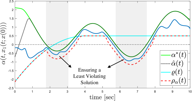
Figure 3: The evolution of $\alpha(t,x_{1}(t;x(0)))$ under the consolidating constraint (13), where $\rho_{\alpha}(t)$ is determined by (33). The adaptation of $\rho_{\alpha}(t)$ (dashed line) based on the evolution of $\hat{\alpha}(t)$ in (31b) (dotted line) allows for deviations of $\rho_{\alpha}(t)$ from the nominal lower bound function $\varrho(t)$ in (32). Consequently, satisfaction of (13) during the time intervals when $\alpha^{\ast}(t)<0$ (shaded intervals) results in a least violating solution. In this illustrative example, $\hat{\alpha}(t)$ provides a reliable estimate of $\alpha^{\ast}(t)$, and the parameters used for this illustration are $\mu=0.45$, $\varrho_{\infty}=0.5$, and $T=4$.

The logic behind the design in (32), (33) and (34) is summarized as follows: first, $\varrho(t)$ in (32) is designed as the nominal lower bound on $\alpha(t,x_{1}(t;x(0)))$ to address the user’s desired specifications regarding the satisfaction of the time-varying output constraints while ignoring whether these constraints are feasible or not for all time. Next, $\rho_{\alpha}(t)$ in (33) is designed as a convex combination of two terms such that when $\hat{\alpha}(t)-\varrho(t)>\mu$, we obtain the nominal lower bound behavior $\rho_{\alpha}(t)=\varrho(t)$. Otherwise, when $\hat{\alpha}(t)-\varrho(t)<0$, we get $\rho_{\alpha}(t)=\hat{\alpha}(t)-\mu$. The transition between these two modes is achieved through the smooth switch (34). Note that since (33) is a convex combination, $\rho_{\alpha}(t)$ always takes a value between $\varrho(t)$ and $\hat{\alpha}(t)-\mu$ during the transition phase where $0\leq\varphi(t)\leq\mu$. In particular, by employing (33), we allow the lower bound $\rho_{\alpha}(t)$ in (13) to deviate from its nominal behavior $\varrho(t)$ in order to achieve a minimum user-defined gap of $\mu$ with respect to $\hat{\alpha}(t)$. Fig. 3 illustrates the behavior of $\rho_{\alpha}(t)$ in (33).

Lemma 4

Let $\tilde{e}\coloneqq\alpha^{\ast}(t)-\hat{\alpha}(t)$. If $\alpha^{\ast}(t)<0$ and $\varrho(t)\geq 0$ for all $t\in I$, where $I$ is some unknown time interval, then the satisfaction of (13) under $\rho_{\alpha}(t)$ given by (33) guarantees a least violating solution with the gap of $\mu^{\ast}=\tilde{e}+\mu$.

Proof:

First, note that since $\hat{\alpha}(t)=\alpha(t,\tilde{x}_{1})\leq\alpha^{\ast}(t),\forall t\geq 0$, we always have $\tilde{e}\geq 0$. Given the conditions in the lemma it is easy to verify that $\varphi(t)=\hat{\alpha}(t)-\varrho(t)<0$ for all $t\in I$. Hence, from (33) and (34) we get $\rho_{\alpha}(t)=\hat{\alpha}(t)-\mu$. Consequently, the satisfaction of (13) leads to $\hat{\alpha}(t)-\mu<\alpha(t,x_{1}(t;x(0))),\forall t\in I$, which is equivalent to $\alpha^{\ast}(t)-\mu^{\ast}<\alpha(t,x_{1}(t;x(0))),\forall t\in I$, with $\mu^{\ast}=\tilde{e}+\mu$. ∎

From Lemma 4, it is evident that the gap of the obtained least violating solution through utilizing (33) in (13) is affected by $\tilde{e}$ and the tunable constant $\mu>0$ in (33). In particular, the better $\hat{\alpha}(t)$ estimates $\alpha^{\ast}(t)$, the smaller the gap $\mu^{\ast}$ becomes.

Consider the case where $\alpha^{\ast}(t)>0,\forall t\in I$, indicating that the time-varying constrained set $\Omega(t)$ is feasible for all $t\in I$, and further assume that $\alpha^{\ast}(t)-\varrho(t)>\mu,\forall t\in I$. In this scenario, when $\hat{\alpha}(t)$ poorly estimates $\alpha^{\ast}(t)$, a situation may arise where $\varphi=\hat{\alpha}(t)-\varrho(t)\leq\mu$, or particularly, $\varphi<0$ in (34). Consequently, $\rho_{\alpha}(t)$ in (33) might not effectively follow the intended behavior designed by $\varrho(t)$ for all $t\in I$. This discrepancy can lead to a certain degree of conservativeness in fulfilling the output constraints. To clarify, even when the constraints are feasible at all time, enforcing (13) under (33) might not guarantee constraint satisfaction if $\hat{\alpha}(t)$ has a very poor performance in estimating $\alpha^{\ast}(t)$. Therefore, it is crucial to properly tune the parameter $k_{\alpha}$ in (31b) to enhance the performance of (31b) especially when $\alpha^{\ast}(t)$ does not vary slowly enough with time. It is also important to emphasize that although $\tilde{x}_{1}(0)$ in (31b) can be set arbitrarily, it is recommended to select $\tilde{x}_{1}(0)$ such that $\alpha(0,\tilde{x}_{1}(0))>\alpha(0,x_{1}(0;x(0)))$, which helps in reducing the conservatism in satisfying the output constraints. As described in Subsection IV-A, it is better to select $\tilde{x}_{1}(0)$ such that $\hat{\alpha}(0)=\alpha(0,\tilde{x}_{1}(0))$ becomes closer to $\alpha^{\ast}(0)$.

Finally, note that the dynamical system (31b), given an initialization $\tilde{x}_{1}(0)$, runs in parallel with the closed-loop system dynamics (1). It generates $\hat{\alpha}(t)$ at each time instant $t$, which is then used in the (online) computation of $\rho_{\alpha}(t)$ in (33). Recall that $\rho_{\alpha}(t)$ is utilized in the control law $u(t,x)$, specifically in the first intermediate control (III-D). Therefore, the gradient flow dynamic (31b) is connected to the closed-loop system in a cascaded form (see Fig. 4), and thus is independent of (1).

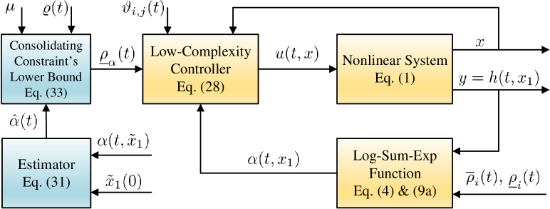
Figure 4: Cascaded control architecture under the estimation scheme (31b) and online computation of $\rho_{\alpha}(t)$ in (33).

To conclude this section we show that the results stated in Theorem 1 still hold under $\rho_{\alpha}(t)$ given in (33). In this regard, to ensure the boundedness of $\hat{\alpha}(t)$ in (31b), we require the following technical assumption:

Assumption 9

There exist $\pi_{\alpha}>0$ such that $|\dot{\alpha}^{\ast}(t)|\leq\pi_{\alpha}$ and $k_{c}>0$ such that $\Lambda(t,\tilde{x}_{1})\coloneqq\frac{\partial\alpha(t,\tilde{x}_{1})}{\partial t}+k_{\alpha}\|\nabla_{\tilde{x}_{1}}\alpha(t,\tilde{x}_{1})\|^{2}$ is coercive (radially unbounded) in $\tilde{x}_{1}$ for all $k_{\alpha}\geq k_{c}$.

Theorem 2

Consider the estimation scheme (31b) with an arbitrary initialization $\tilde{x}_{1}(0)$ and let $\rho_{\alpha}(t)$ be given by (33). Moreover, suppose that $\varrho_{0}$ in (32) is selected such that $\varrho_{0}<\alpha(0,x_{1}(0))$. Under Assumptions 4, 5, 6, and 9 $\rho_{\alpha}(t)$ attains Properties (i) and (ii) mentioned in Subsection III-B. Moreover, $\dot{\rho}_{\alpha}(t)$ is bounded. Therefore, under the requirements stated in Theorem 1, the control law (28) ensures the satisfaction of $\rho_{\alpha}(t)<\alpha(t,x_{1}(t;x(0)))$ and the boundedness of all closed-loop signals for all time.

Proof:

See Appendix E. ∎

V Simulation Results

In this section, we present two simulation examples to validate the proposed control approach. The first example demonstrates our method’s effectiveness in addressing problems that are already solvable using existing approaches, such as the PPC method, where the considered time-varying output constraints are decoupled. Subsequently, we offer an example involving coupled time-varying constraints, which cannot be accommodated by previous approaches.

In the upcoming simulation examples, we will consider a mobile robot operating in a 2-D plane (refer to Fig. 5) with kinematics and dynamics expressed by the following equations:

$$\begin{cases}\dot{p}_{c}=S(\theta)\zeta\\ \bar{M}\dot{\zeta}+\bar{D}\zeta=\bar{u}+\bar{d}(t)\end{cases}\!\!\!\!\!\!,~{}\begin{aligned} S(\theta)\!=\!\!\left[\!\!\!\begin{array}[]{ccc}\cos\theta&\!\!\sin\theta&\!\!0\\ 0&\!\!0&\!\!1\end{array}\!\!\!\right]^{\!\!\top}\!\!\!.\!\!\!\!\!\!\!\end{aligned}$$ (35)

Here, $p_{c}=[x_{c},y_{c},\theta]^{\top}$ represents the position and orientation of the body frame ${C}$ relative to the reference frame ${O}$. The vector $\zeta=[v_{T},\dot{\theta}]^{\top}$ includes the translational speed $v_{T}$ along the direction of $\theta$ and the angular speed $\dot{\theta}$ about the vertical axis passing through $C$. The matrices involved are defined as follows: $\bar{M}=\mathrm{diag}(m_{R},I_{R})$, where $m_{R}$ and $I_{R}$ represent the mass and moment of inertia of the robot about the vertical axis, respectively. The input $\bar{u}$ denotes the force/torque-level control inputs, $\bar{D}=\mathrm{diag}(\bar{D}_{1},\bar{D}_{2})$ is a constant damping matrix, and $\bar{d}(t)$ is the vector of bounded external disturbances.

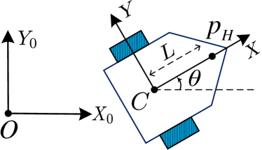
Figure 5: Mobile robot.

To address the under-actuated nature of (35) and avoid nonholonomic constraints, we transform it with respect to the hand position $p_{H}\coloneqq[x_{c},y_{c}]^{\top}+L[\cos\theta,\sin\theta]^{\top}$ (as shown in Fig. 5). This transformation leads to an equivalent Euler-Lagrangian dynamics in state-space form:

$$\!\!\dot{x}_{1} =x_{2},$$ (36)

$$\!\!\dot{x}_{2} =M(x_{1})^{-1}\big{(}-C(x_{1},x_{2})x_{2}-D(x_{1})x_{2}+u+d(t)\big{)}.\!\!\!$$

Here, $x_{1}$ corresponds to the hand position of the mobile robot ($x_{1}=p_{H}$), and $x_{2}$ represents its velocity. The matrices $M(x_{1})$, $C(x_{1},x_{2})$, and $D(x_{1})$ are locally Lipschitz continuous functions of their arguments. The relationships between the parameters in (36) and those in (35) are given by: $M=\Upsilon^{\top}\bar{M}\Upsilon$, $C=\Upsilon^{\top}\bar{M}\dot{\Upsilon}$, $D=\Upsilon^{\top}\bar{D}\Upsilon$, $d(t)=\Upsilon^{\top}\bar{d}(t)$, and $u=\Upsilon^{\top}\bar{u}$, where $\Upsilon=\left[\begin{smallmatrix}\cos\theta&\sin\theta\\ -(\sin\theta)/L&(\cos\theta)/L\end{smallmatrix}\right]$ [68]. It is worth noting that (36) can be viewed as a specific form of (1) with $n=2$ and $r=2$ and it is not difficult to verify that Assumptions 1, 2, and 3 hold for (36). In the simulations we set $m_{R}=3.6$, $I_{R}=0.0405$, $\bar{D}_{1}=0.3$, $\bar{D}_{2}=0.04$, $L=0.2$, and $\bar{d}(t)=[0.75\sin(3t+\tfrac{\pi}{3})+1.5\cos(t+\tfrac{3\pi}{7}),-2.4\exp(\cos(t+\tfrac{\pi}{3})+1)\sin(t)]^{\top}$.

V-A Decoupled Time-Varying Constraints

In our first simulation example, we will focus on trajectory tracking for the mobile robot described by (36). The desired trajectory is $x_{1}^{d}(t)=[4.2\cos(0.47t),4.2\sin(0.47t)]^{\top}$. Our goal is to enforce specific performance funnel constraints on tracking errors, defined as follows: $-\rho_{i}(t)<x_{1,i}-x_{1,i}^{d}(t)<\rho_{i}(t)$ for $i\in\mathcal{I}_{1}^{2}$ and all $t\geq 0$. Here, $\rho_{1}(t)$ and $\rho_{2}(t)$ are strictly positive, time-varying performance bounds. Without loss of generality, we assume $\rho_{1}(t)=\rho_{2}(t)=(1.75-0.3)\exp(-0.35t)+0.3$.

To express these requirements analogously to the problem formulation in Section II, we consider $y=h(x_{1})=x_{1}$ for the dynamics (36) under the following funnel constraints: $\underline{\rho}_{i}(t)\coloneqq-\rho_{i}(t)+x_{1,i}^{d}(t)<x_{1,i}<\rho_{i}(t)+x_{1,i}^{d}(t)\eqqcolon\overline{\rho}_{i}(t)$ for $i\in\mathcal{I}_{1}^{2}$ and all $t\geq 0$. Note that $h(x_{1})$ readily satisfies Assumptions 4 and 5. Moreover, the above funnel constraints resemble a time-varying box constraint in the $x_{1}$ space (i.e., Assumption 6 holds). As $\rho_{1}(t)$ and $\rho_{2}(t)$ are strictly positive, both funnel constraints are well-defined and feasible. Furthermore, these two funnel constraints are decoupled, as each one imposes time-varying upper and lower bounds on independent state variables, namely $x_{1,1}$ and $x_{1,2}$. This feature is also evident by verifying that Condition II of Lemma 3 holds. Satisfaction of Condition II of Lemma 3 also indicates that Assumption 8 is valid. Now since the aforementioned funnel constraints are well-defined and decoupled, they are mutually satisfiable for all time. Therefore, the constrained set $\bar{\Omega}(t)$ defined in (8) is guaranteed to be feasible for all $t\geq 0$.

In this specific example, one can reasonably assume that Assumption 7 holds, given that $\bar{\Omega}(t)$ remains feasible for all time and does not become excessively tight over certain time intervals (i.e., having overly stringent time-varying constraints). Indeed, by selecting a sufficiently large $\nu$ in (9) one can get a closer under-approximation of $\bar{\Omega}(t)$, which provides more confidence on feasibility of $\Omega(t)$. Satisfaction of Assumption 7 allows us to use the suggested design of $\rho_{\alpha}(t)$ in (14) for consolidating constraint (13).

The numerical values of the parameters used to implement control law (28) are provided in Table I. It is important to note that, as per the guidelines outlined in Subsections III-C and III-D, the values of $\rho_{0}$ and $\vartheta_{2,j}^{0}$, $j\in\mathcal{I}_{1}^{2}$ in Table I, are determined based on the initial condition $x(0)$ of the transformed mobile robot dynamics in (36). Henceforth, we use $x_{1}(t)$ instead of $x_{1}(t;x(0))$ for brevity. Fig. 6 shows the evolution of $\alpha(t,x_{1}(t))$ and the tracking errors of the mobile robot’s hand position under (28) for two scenarios.

Eq. no	Parameter(s)
(9a)	$\nu=10$
(14)	$T=3$, $\beta=0.3$, $\rho_{\infty}=0$, $\rho_{0}<\alpha(0,x_{1}(0))$
(16)	$\upsilon=8$
(III-D)	$k_{1}=1$
(21)	$\vartheta_{2,j}^{\infty}=0.1$, $l_{2,j}=1$, $\vartheta_{2,j}^{0}>|e_{2,j}(0,\bar{x}_{2}(0))|,j\in\mathcal{I}_{1}^{2}$
(III-D)	$k_{2}=1$

TABLE I: Numerical values of the parameters involved in control law (28).

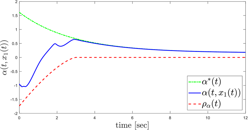
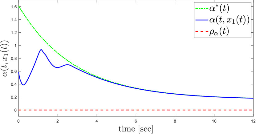
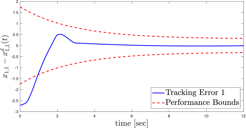
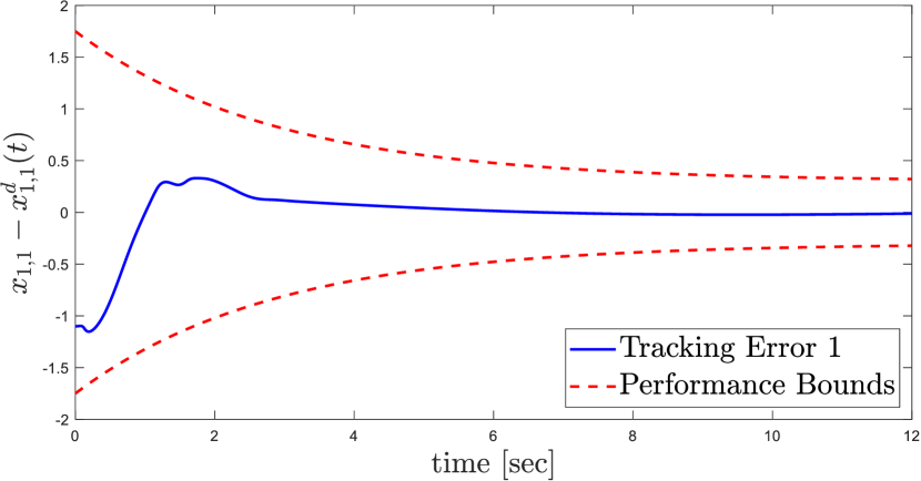
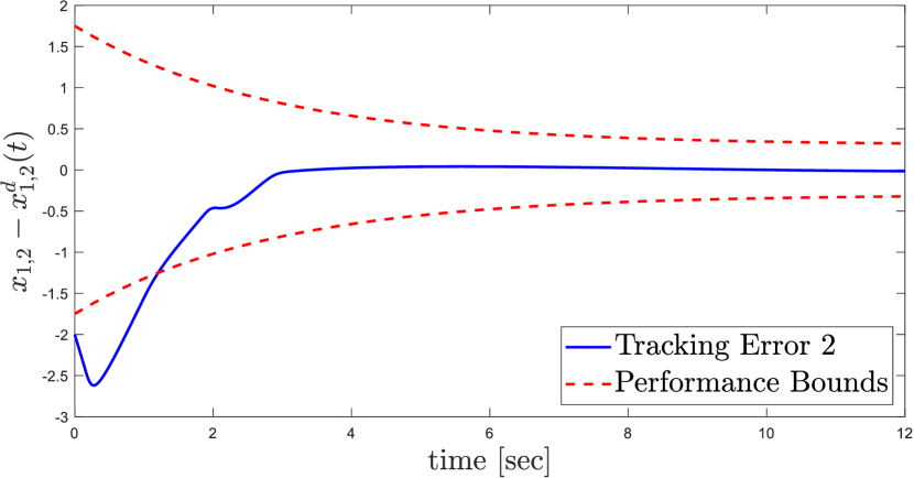
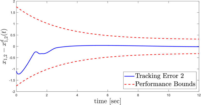
(a)

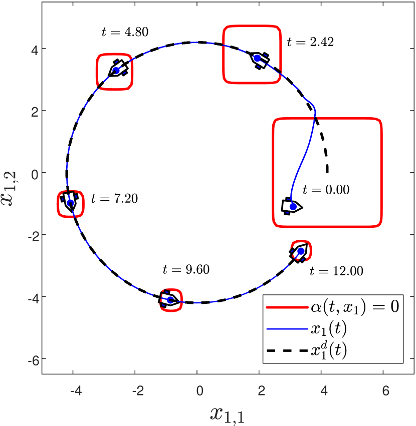
(b)

Figure 6: Trajectory tracking of the mobile robot under prescribed performance conditions. (a) The scenario where the tracking errors performance specifications are not initially satisfied. (b) The situation in which the performance specifications are initially met.

In the first scenario (Fig. 6(a)), since $\alpha(0,x_{1}(0))<0$ the robot’s initial position does not initially satisfy the prescribed performance bounds on the tracking errors ($x_{1}(0)\notin\bar{\Omega}(0)$). However, by enforcing (13) under $\rho_{\alpha}(t)$ in (14) and applying (28), we observe that $\alpha(t,x_{1}(t))$ becomes and remains positive within the user-defined finite time limit of $T=3$ seconds. This signifies the achievement of the tracking error performance specifications within 3 seconds.

In the second scenario (Fig. 6(b)), where $\alpha(0,x_{1}(0))>0$, the performance bounds on the tracking errors are initially satisfied ($x_{1}(0)\in\bar{\Omega}(0)$). By maintaining $\alpha(0,x_{1}(t))$ positive, we ensure the continuous fulfillment of the tracking errors’ specifications throughout the simulation. It is worth noting that, as anticipated, $\alpha^{\ast}(t)$ remains positive for all time, which indicates the feasibility of $\Omega(t)$ for all time. Note that, $\alpha^{\ast}(t)$ is unknown to the control system and is included in the figures solely for the purpose of verifying the simulation results. The value of $\alpha^{\ast}(t)$ at each time step is obtained through solving optimization (30) offline for a dense set of time instances.

Lastly, Fig. 6 (bottom) provides a visual representation of the simulation results through snapshots of the mobile robot’s hand position trajectory $x_{1}(t)$ along with the time-varying constrained set $\Omega(t)$ for both scenarios (recall that $\partial\mathrm{cl}(\Omega(t))=\{x_{1}\in\mathbb{R}^{2}\mid\alpha(t,x_{1})=0\}$).

The simulation results presented above highlight a key advantage of our proposed control methodology. Unlike conventional PPC and TVBLF-based control design approaches, which necessitate the initial satisfaction of the (output) constraints for their effective implementation, our approach operates without such restrictions.

V-B Coupled Time-Varying Constraints

For our second simulation example we consider coupled time-varying (output) constraints, for which previous approaches (FC, PPC, TVBLF-based control) are not applicable. Moreover, previous approaches cannot ensure a least violating solution (as per (29)) when constraint infeasibilities arise.

Consider the transformed mobile robot dynamics in (36) with the output map $y=h(t,x_{1})=\left[h_{1}(t,x_{1}),h_{2}(t,x_{1}),h_{3}(t,x_{1})\right]^{\top}$, for which we assume the following (coupled) time-varying constraints: $\underline{\rho}_{1}(t)<h_{1}(t,x_{1})<\overline{\rho}_{1}(t)$ (funnel constraint), $\underline{\rho}_{2}(t)<h_{2}(t,x_{1})$ (LBO constraint), and $h_{3}(t,x_{1})<\overline{\rho}_{3}(t)$ (UBO constraint), where $\underline{\rho}_{1}(t)=-0.7-\sin(0.4t)$, $\overline{\rho}_{1}(t)=1.1+3\sin(0.45t)$, $\underline{\rho}_{2}(t)=-1-0.5\cos(0.3t)$, and $\overline{\rho}_{3}(t)=0.5+\sin(0.4t)$. Moreover, let $h_{1}(t,x_{1})=x_{1,1}-o_{1}(t)$, $h_{2}(t,x_{1})=c_{1}(t)(x_{1,1}-o_{1}(t))^{2}+c_{2}(t)(x_{1,2}-o_{2}(t))+c_{3}(t)(x_{1,1}-o_{1}(t))$, and $h_{3}(t,x_{1})=c_{4}(t)(x_{1,1}-o_{1}(t))^{2}+(x_{1,2}-o_{2}(t))$, in which $o_{1}(t)=5\cos(0.28t),o_{2}(t)=5\sin(0.28t)$, $c_{1}(t)=-2+2\cos(t)$ , $c_{2}(t)=1+0.5\sin(0.7t)$, $c_{3}(t)=\sin(0.4t)$, and $c_{4}(t)=1-\cos(0.5t)$ are all bounded continuously differentiable functions of time. The time-varying output map $h(t,x_{1})$ satisfies Assumptions 4 and 5. Furthermore, due to the way the constraints are designed, the set $\bar{\Omega}(t)$ (and consequently $\Omega(t)$) remains bounded for all time (Assumption 6). Moreover, it can be verified that the constraints fulfill Condition I of Lemma 3, thus confirming the validity of Assumption 8. In simple terms, these constraints define a bounded time-varying region that the mobile robot’s (hand) position should enter and remain within for all time (i.e., a time-varying region tracking problem). Nevertheless, we did not assume that the constrained region is always feasible. Therefore, we utilize the proposed estimation scheme (31b) along with $\rho_{\alpha}(t)$ given by (33) for the consolidating constraint (13).

For the simulations of this subsection, all numerical values used for the control law (28) match those in Table I, with the only difference being that $\rho_{\alpha}(t)$ follows (33). Specifically, we set $\mu=0.2$ in (33), and the parameters for $\varrho(t)$ in (32) are set to $\varrho_{0}<\alpha(0,x_{1}(0))$, $\varrho_{\infty}=0.5$, $T=3$, and $\beta=0.3$. Building on the discussion in Subsection IV-A, we conduct two simulations to highlight how the performance of the estimation scheme (31b) impacts constraint satisfaction under control law 28. In these simulations, we explore two cases: setting $k_{\alpha}=4$ and $k_{\alpha}=1$ in (31a). Both simulations assume that the initial condition for the estimator (31a) is the same as the initial hand position of the mobile robot, i.e., $\tilde{x}_{1}(0)=x_{1}(0)$, leading to $\hat{\alpha}(0)=\alpha(t,x_{1}(0))$.

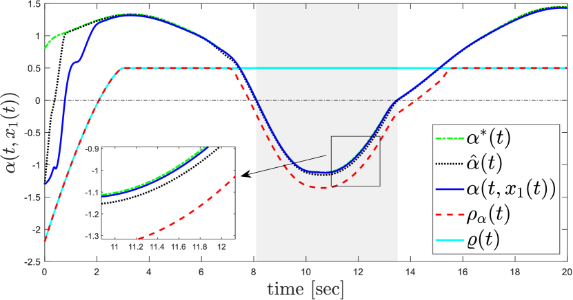
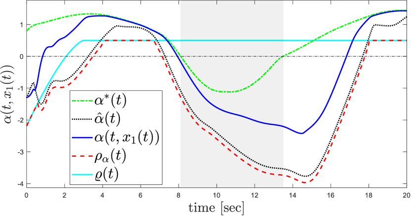
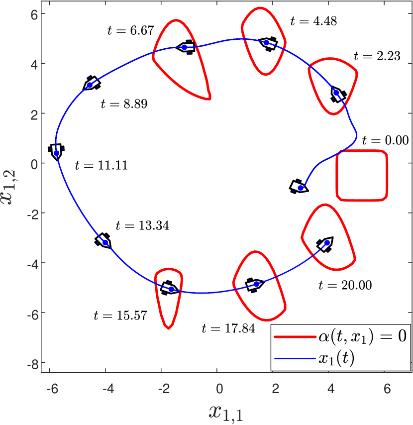
(a)

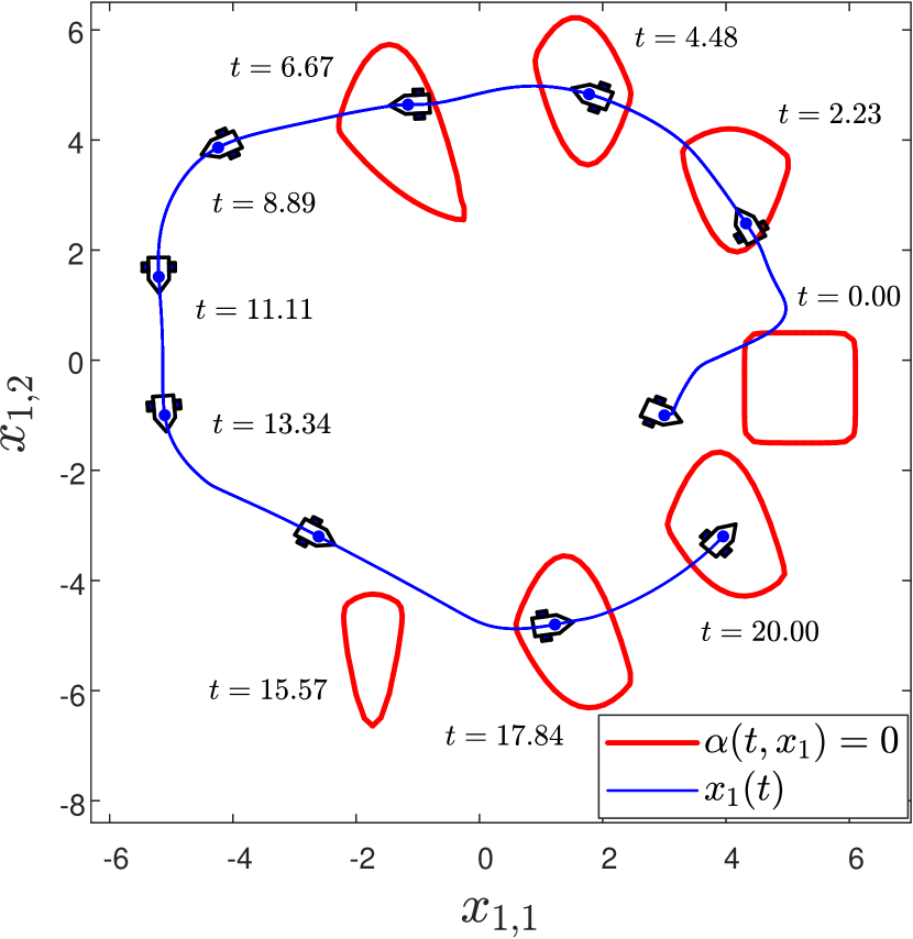
(b)

Figure 7: Time-varying region tracking of the mobile robot. (a) With an estimator gain of $k_{\alpha}=4$ in (31a) minimal conservative behavior is achieved in satisfaction of the time-varying constraints (or region tracking), attributed to the estimator’s good performance in estimating (unknown) $\alpha^{\ast}(t)$. Moreover, a least violating solution is ensured with a small gap whenever the constraints become infeasible (empty region). (b) A reduced estimator gain of $k_{\alpha}=1$ leads to a least violating solution with a large gap and adversely impacts the control law’s performance, resulting in a more conservative satisfaction of time-varying constraints.

Fig. 7(a) (top) shows the evolution of $\alpha(t,x_{1}(t))$ under control law (28) with $k_{\alpha}=4$ in the estimation scheme (31a). After a brief transient period, the estimator’s output ($\hat{\alpha}(t)$) closely follows $\alpha^{\ast}(t)$, such that the estimation error remains small for all time. Additionally, thanks to the satisfaction of consolidating constraint (13), time-varying output constraints are guaranteed to be met with a margin of $\varrho_{\infty}=0.5$ after a user-defined $T=3$ seconds. However, roughly between $t=8$ and $t=14$ (shaded interval), $\alpha^{\ast}(t)<0$, indicating that the constraints become temporarily infeasible. During this time, the proposed $\rho_{\alpha}(t)$ (33) diverts from the nominal lower bound $\varrho(t)$ to ensure a least violating solution. When the constraints become feasible again ($\alpha^{\ast}(t)>0$), $\rho_{\alpha}(t)$ quickly returns to the nominal constraint satisfaction requirement i.e., $\rho_{\alpha}(t)=\varrho_{\infty}=0.5$. Finally, in Fig. 7(a) (bottom), snapshots of the mobile robot’s hand position are shown along with the constrained region. Note that, the constrained region is shown only when it is feasible (nonempty).

The same simulation scenario is repeated with a lower gain, $k_{\alpha}=1$ in (31a), and the results are presented in Fig. 7(b). This reduced gain leads to a poorer performance in estimating $\alpha^{\ast}(t)$. In Fig. 7(b) (top), we can see that the evolution of $\rho_{\alpha}(t)$ is influenced by $\hat{\alpha}(t)$, initially deviating from the nominal lower bound $\varrho(t)$ until $t=4$. However, as this deviation is not significant it turns out that the controller is still capable of meeting the user-defined specifications for constraints satisfaction by maintaining $\alpha(t,x_{1}(t))$ above the nominal lower bound $\varrho(t)$ for over 7 seconds (although only $\rho_{\alpha}(t)<\alpha(t,x_{1}(t))$ is guaranteed by the proposed controller). As the time-varying constraints tend to become infeasible (shaded interval), $\alpha^{\ast}(t)$ rapidly decreases, which induces a significant divergence between $\rho_{\alpha}(t)$ and $\varrho(t)$ due to a large estimation error. As a result, the controller can only ensure a least violating solution with a considerably large gap. Recall that, as per Lemma 4, the gap for the least violating solution is given by $\mu^{\ast}=\tilde{e}+\mu$, where $\tilde{e}=\alpha^{\ast}(t)-\hat{\alpha}(t)\geq 0$ represents the estimation error. From Fig. 7(b) (top), it is evident that, even when the constraints become feasible again, owing to a rapid increase of $\alpha^{\ast}(t)$ a large estimation error continues to persist for some time, which hinders $\rho_{\alpha}(t)$ from approaching $\varrho(t)$. This phenomenon makes the controller to present a more conservative constraint satisfaction behavior. This is more evident in Fig. 7(b) (bottom), where the mobile robot is still out of the (feasible) constrained region at $t=15.57$. This simulation underscores the direct impact of the estimator’s performance on the control law. Therefore, if one expects that $\alpha^{\ast}(t)$ can change rapidly, careful tuning of the gain for estimator (31a) becomes essential.

VI Conclusions

This work introduced a novel low-complexity feedback control design for high-order uncertain MIMO nonlinear systems with multiple (potentially coupled) time-varying output constraints. Our method addresses these constraints by interpreting their satisfaction as the fulfillment of a single consolidating constraint related to the signed distance with respect to the boundary of the time-varying constrained set. We have shown that by dynamically adjusting the lower bound of the consolidating constraint, our method ensures a least violating solution when the time-varying constraints become infeasible for an unknown time interval. Moreover, it overcomes the limitations of existing feedback control design approaches when dealing with coupled time-varying output constraints. As a result, it can be applied to a broader range of applications. Future work may involve employing this method in various applications and further investigation of its capabilities and limitations, especially when Assumption 8 does not hold.

Appendix A Proof of Lemma 1

To start with, notice that all $\overline{\rho}_{i}(t),\underline{\rho}_{i}(t)$ in (4) are bounded, and based on Assumption 5, $|h_{i}(t,x_{1})|\leq\bar{h}_{i}(x_{1}),i\in\mathcal{I}_{1}^{m}$ holds. Therefore, $\psi_{i}(t,x_{1}),i\in\mathcal{I}_{1}^{m}$ are bounded for all $t\geq 0$ and any fixed $x_{1}$. As a result, $\bar{\alpha}:\mathbb{R}_{\geq 0}\times\mathbb{R}^{n}\rightarrow\mathbb{R}$ in (7) is bounded for all $t\geq 0$ and any fixed $x_{1}$. Let $\bar{\alpha}_{t}(x_{1})\coloneqq\bar{\alpha}(t,x_{1})$. According to Assumption 6, $-\bar{\alpha}_{t}(x_{1})$ is coercive in $x_{1}$ for each $t$. Therefore, by [69, Proposition 2.9], all super-level sets $\bar{\alpha}_{t}(x_{1})\geq c$, where $c\in\mathbb{R}$, are bounded for each $t$. Furthermore, based on Assumption 6 and [65, Theorem 1.4.4, p. 27], we can infer that there exists a time-dependent constant $\bar{c}(t)\in\mathbb{R}$ such that the super-level sets $\bar{\alpha}_{t}(x_{1})>\bar{c}(t)$ are empty. This implies that $\bar{\Omega}(t)$ in (8) is bounded, and in particular, it is empty if $\bar{c}(t)<0$ at time $t$. Moreover, from (9b) we can verify that $-\bar{\alpha}(t,x_{1})$ is coercive if and only if $-\alpha(t,x_{1})$ is coercive. As a result, we can apply similar arguments as above to establish the boundedness of $\Omega(t)$.

Appendix B Proof of Lemma 2

Using (7), we can determine whether $-\bar{\alpha}(t,x_{1})$ is coercive by verifying that, for each time instant $t$, at least one of the functions $\psi_{i}(t,x_{1})$ in (4) approaches $-\infty$ as $\|x_{1}\|\rightarrow+\infty$ (along any path on $\mathbb{R}^{n}$). Note that $-\alpha(t,x_{1})$ in (9) is also coercive under the same condition. Since the functions $\psi_{i}(t,x_{1}),i\in\mathcal{I}_{1}^{m+p}$ in (4) are bounded for all $t\geq 0$ and any fixed $x_{1}$ (see proof of Lemma 1), we can interpret this requirement in terms of $h_{i}(t,x_{1})$. Specifically, if there exists an $i\in\mathcal{I}_{1}^{p}$ such that $h_{i}(t,x_{1})\rightarrow\pm\infty$ for each time instant $t$, then it ensures that $\psi_{2i-1}(t,x_{1})\rightarrow-\infty$ or $\psi_{2i}(t,x_{1})\rightarrow-\infty$ in (4a) and vice versa. To simplify the verification process, we only need to check whether $\|h_{f}(t,x_{1})\|\rightarrow+\infty$ for each time instant $t$ and along a path on $\mathbb{R}^{n}$ as $\|x_{1}\|\rightarrow+\infty$. From (4b), we can also see that if there exists a $j\in\mathcal{I}_{p+1}^{p+q}$ such that $h_{j}(t,x_{1})\rightarrow-\infty$ for each time instant $t$, then there exists an $i\in\mathcal{I}_{2p+1}^{2p+q}$ such that $\psi_{i}(t,x_{1})\rightarrow-\infty$ and vice versa. Similarly, if there exists a $j\in\mathcal{I}_{p+q+1}^{m}$ such that $h_{j}(t,x_{1})\rightarrow+\infty$ for each time instant $t$, then there exists an $i\in\mathcal{I}_{2p+q+1}^{p+m}$ such that $\psi_{i}(t,x_{1})\rightarrow-\infty$ and vice versa. In summary, if along any path on $\mathbb{R}^{n}$ as $\|x_{1}\|\rightarrow+\infty$ at least one of the conditions I-III in the lemma holds, then $-\bar{\alpha}(t,x_{1})$ (resp. $-\alpha(t,x_{1})$) is coercive and vice versa.

Appendix C Proof of Lemma 3

Case I: Consider $\alpha(t,x_{1})$ in (9). First, note that since $\psi_{i}(t,x_{1}),i\in\mathcal{I}_{1}^{m+p}$ are concave functions in $x_{1}\in\mathbb{R}^{n}$ at time $t$ then as $\nu>0$, $-\nu\,\psi_{i}(t,x_{1}),i\in\mathcal{I}_{1}^{m+p}$ are convex at time $t$. Moreover, from [70, Section 3.5] it is known that $e^{-\nu\,\psi_{i}(t,x_{1})},i\in\mathcal{I}_{1}^{m+p}$ are log-convex functions. Hence, $\sum_{i=1}^{m+p}e^{-\nu\,\psi_{i}(t,x_{1})}$ is log-convex. Consequently, $\alpha(t,x_{1})$ in (9) is a concave function at time $t$. Furthermore, since $\alpha(t,x_{1})$ has bounded level sets, from Assumption 6, it attains a well-defined global maximum (i.e., the global maximum exists). Therefore, one can conclude that every critical point of $\alpha(t,x_{1})$ is a global maximizer at time $t$.

Case II: Here, we first establish that under the given conditions $\alpha(t,x_{1})$ attains only one critical point and then we show that the critical point is the (unique) global maximizer of $\alpha(t,x_{1})$. Recall that the critical points of $\alpha(t,x_{1})$ are obtained by solving $\nabla_{x_{1}}\alpha(t,x_{1})=0$. Given the assumed ordering of constraint types in (4) one can write $\alpha(t,x_{1})$ in (9) as follows:

$$\alpha(t,x_{1})=-\dfrac{1}{\nu}\ln\Big{(}\!\sum_{i=1}^{p}e^{-\nu\,(h_{i}(t,x_{1})-\underline{\rho}_{i}(t))}\!+\!e^{-\nu\,(\overline{\rho}_{i}(t)-h_{i}(t,x_{1}))}$$

$$+\!\!\sum_{i=p+1}^{p+q}\!e^{-\nu\,(h_{i}(t,x_{1})-\underline{\rho}_{i}(t))}+\!\!\!\sum_{i=p+q+1}^{m}\!\!\!e^{-\nu\,(\overline{\rho}_{i}(t)-h_{i}(t,x_{1}))}\Big{)}.\!\!\!\!\!\!$$ (37)

Using (C) and (9), and after some calculations, we can obtain $\nabla_{x_{1}}\alpha(t,x_{1})$ in a compact form as:

$$\nabla_{x_{1}}\alpha(t,x_{1})=J^{\top}(t,x_{1})\,\gamma(t,x_{1})\,e^{\nu\alpha(t,x_{1})},$$ (38)

where $J(t,x_{1})=\frac{\partial h(t,x_{1})}{\partial x_{1}}\in\mathbb{R}^{m\times n}$ is the Jacobian of $y=h(t,x_{1})$, and $\gamma(t,x_{1})\coloneqq\mathrm{col}(\gamma_{i}(t,x_{1}))\in\mathbb{R}^{m}$, in which $\gamma_{i}(t,x_{1}),i\in\mathcal{I}_{1}^{m}$ are given by:

$$e^{-\nu\,(h_{i}(t,x_{1})-\underline{\rho}_{i}(t))}-e^{-\nu\,\left(\overline{\rho}_{i}(t)-h_{i}(t,x_{1})\right)}, i\in\mathcal{I}_{1}^{p}$$ (39a)

$$e^{-\nu\,(h_{i}(t,x_{1})-\underline{\rho}_{i}(t))}, i\in\mathcal{I}_{p+1}^{p+q}$$ (39b)

$$-e^{-\nu\,\left(\overline{\rho}_{i}(t)-h_{i}(t,x_{1})\right)}, i\in\mathcal{I}_{p+q+1}^{m}$$ (39c)

Notice that in (38) $e^{\nu\alpha(t,x_{1})}>0$, therefore, $\nabla_{x_{1}}\alpha(t,x_{1})=0$ if and only if $J^{\top}(t,x_{1})\,\gamma(t,x_{1})=0$. If $m=n$ and each output constraint is a funnel constraint (i.e., $p=m=n$) then all $\gamma_{i}(t,x_{1})$ will be given by (39a). In this case, $J(t,x_{1})\in\mathbb{R}^{n\times n}$ in (38) is a square matrix. If at time instance $t$ we have $\mathrm{rank}(J)=n$ for all $x\in\mathbb{R}^{n}$, then $J^{\top}(t,x_{1})\,\gamma(t,x_{1})=0$ holds if and only if $\gamma(t,x_{1})=0$ at time $t$. Therefore, under the above conditions, at time instant $t$, we get $\nabla_{x_{1}}\alpha(t,x_{1})=0$ if and only if $\gamma_{i}(t,x_{1})=0,\forall i\in\mathcal{I}_{1}^{p}$. Owing to (39a) this leads to having $h_{i}(t,x_{1})=0.5(\overline{\rho}_{i}(t)+\underline{\rho}_{i}(t)),\forall i\in\mathcal{I}_{1}^{p}$, hence, we get the following system of nonlinear equations:

$$F(t,x_{1})\coloneqq h(t,x_{1})-0.5\left(\overline{\rho}(t)+\underline{\rho}(t)\right)=0,$$ (40)

with $\overline{\rho}(t)\coloneqq\mathrm{col}(\overline{\rho}_{i}(t))\in\mathbb{R}^{n}$, $\underline{\rho}(t)\coloneqq\mathrm{col}(\underline{\rho}_{i}(t))\in\mathbb{R}^{n}$, where $F(t,x_{1})$ is $\mathcal{C}^{1}$ in $t$ and $\mathcal{C}^{2}$ in $x_{1}$ owing to the properties of $h(t,x_{1})$, $\overline{\rho}(t)$, and $\underline{\rho}(t)$. Now for each time instant $t$ define $F_{t}(x_{1})\coloneqq F(t,x_{1})$ and recall that in (40) $0.5\left(\overline{\rho}(t)+\underline{\rho}(t)\right)$ is bounded for all time and the elements of $h(t,x_{1})$ do not grow unbounded by the variation of $t$ (Assumption 5). We are interested in checking the existence and uniqueness of the solution to (40) at each time instant $t$, which boils down to checking the existence and uniqueness of the solution to $F_{t}(x_{1})=0$ for each $t$. Since $h(t,x_{1})$ is norm-coercive (i.e., $\|h(t,x_{1})\|\rightarrow+\infty\quad\text{as}\quad\|x_{1}\|\rightarrow+\infty$) then $F_{t}(x_{1})$ is norm-coercive as well. Moreover, from (40) $F_{t}(x_{1})$ has the same Jacobian matrix as $h(t,x_{1})$, which is invertible by assumption. Consequently, all conditions of the global inverse function theorem [71, Collorary] are met, and thus $F_{t}(x_{1})$ is a diffeomorphism at each time instant $t$. Therefore, $F_{t}(x_{1})=0$ or equivalently ${F}(t,x_{1})=0$ has a (single) unique solution $x_{1}^{\ast}(t)$ for each $t$, which is the unique critical point of $\alpha(t,x_{1})$ at time $t$. Note that, since ${F}(t,x_{1})$ is continuous, $x_{1}^{\ast}(t)$ depends continuously on time.

Next, we will show that the unique critical point of $\alpha(t,x_{1})$ at time $t$, i.e., $x_{1}^{\ast}(t)$, is indeed the global maximum point of $\alpha(t,x_{1})$ at time $t$. In this regard, we consider the second derivative test on the critical point’s trajectory of $\alpha(t,x_{1})$. From (38) and followed by matrix differentiation rules [72], we obtain the Hessian matrix of $\alpha(t,x_{1})$, i.e., $\mathcal{H}(t,x_{1})\coloneqq\frac{\partial}{\partial x_{1}}\left(\nabla_{x_{1}}\alpha(t,x_{1})\right)$ as:

(41)

Recall that on the critical point’s trajectory we have $\gamma(t,x_{1}^{\ast}(t))=0$. Hence, evaluating (41) on $x_{1}^{\ast}(t)$ gives:

(42)

From (39a), one can get:

$$\left.\dfrac{\partial}{\partial x_{1}}\left(\gamma(t,x_{1})\right)\right|_{x_{1}=x_{1}^{\ast}(t)}=\Gamma(t,x_{1}^{\ast}(t))\;J(t,x_{1}^{\ast}(t)),$$ (43)

where $\Gamma(t,x^{\ast}(t))\in\mathbb{R}^{n\times n}$ is a negative definite diagonal matrix whose diagonal entries are given by:

$$-\nu\left[e^{-\nu(h_{i}(t,x_{1}^{\ast}(t))-\underline{\rho}_{i}(t))}+e^{-\nu(\overline{\rho}_{i}(t)-h_{i}(t,x_{1}^{\ast}(t)))}\right].$$ (44)

Therefore:

(45)

Notice that $e^{\nu\alpha(t,x_{1}^{\ast}(t))}>0$ for all time. Since $J(t,x_{1}^{\ast}(t))$ is a full rank square matrix and $\Gamma(t,x_{1}^{\ast}(t))$ is a negative definite matrix, one can infer that the Hessian matrix $\mathcal{H}(t,x_{1}^{\ast}(t))$ is negative definite [73]. Therefore, the critical point $x_{1}^{\ast}(t)$ is a local maximizer. Since $x_{1}^{\ast}(t)$ is the unique critical point of $\alpha(t,x_{1})$ at time $t$, we conclude that $x_{1}^{\ast}(t)$ is indeed the (unique) global maximizer of $\alpha(t,x_{1})$ at time $t$.

Appendix D Proof of Theorem 1

First, note that from (19) we have $x_{2}=e_{2}+s_{1}(t,x_{1})$, $x_{3}=e_{3}+s_{2}(t,\bar{x}_{2})$ and $x_{i}=e_{i}+s_{i-1}(t,\bar{x}_{i-1}),i\in\mathcal{I}_{4}^{r}$. Therefore, from (22) and with a slight abuse of notation, we can recursively obtain:

$$x_{2} =\varTheta_{2}^{-1}(t)\,\hat{e}_{2}+s_{1}(t,x_{1}),$$ (46a)

$$x_{3} =\varTheta_{3}^{-1}(t)\,\hat{e}_{3}+s_{2}(t,x_{1},\hat{e}_{2}),$$ (46b)

$$x_{i} =\varTheta_{i}^{-1}(t)\,\hat{e}_{i}+s_{i-1}(t,x_{1},\hat{e}_{2},\ldots,\hat{e}_{i-1}),\quad i\in\mathcal{I}_{4}^{r}.$$ (46c)

From the system dynamics (1) and (46a) one can write:

$$\dot{x}_{1} \coloneqq\phi_{1}(t,x_{1},\hat{e}_{2})$$ (47)

$$=f_{1}(t,x_{1})+G_{1}(t,x_{1})\left(\varTheta_{2}^{-1}(t)\,\hat{e}_{2}+s_{1}(t,x_{1})\right)+w_{1}(t).$$

Taking the time derivative of (15) and utilizing (1) and (46a) yields:

$$\dot{e}_{\alpha} \coloneqq\phi_{\alpha}(t,x_{1},\hat{e}_{2})=\frac{\partial\alpha(t,x_{1})}{\partial x_{1}}\dot{x}_{1}+\frac{\partial\alpha(t,x_{1})}{\partial t}-\dot{\rho}_{\alpha}(t)$$

$$=\frac{\partial\alpha(t,x_{1})}{\partial x_{1}}\Big{[}f_{1}(t,x_{1})+G_{1}(t,x_{1})\left(\varTheta_{2}^{-1}(t)\,\hat{e}_{2}+s_{1}(t,x_{1})\right)$$

$$\quad+w_{1}(t)\Big{]}+\frac{\partial\alpha(t,x_{1})}{\partial t}-\dot{\rho}_{\alpha}(t).$$ (48)

Moreover, differentiating (22) with respect to time and substituting equations (1), (46), and (28) results in:

$$\dot{\hat{e}}_{2} \coloneqq\phi_{2}(t,x_{1},\hat{e}_{2},\hat{e}_{3})$$ (49a)

$$=\varTheta_{2}^{-1}(t)\Big{[}f_{2}(t,x_{1},\hat{e}_{2})+G_{2}(t,x_{1},\hat{e}_{2})\big{(}\varTheta_{3}^{-1}(t)\,\hat{e}_{3}$$

$$\quad+s_{2}(t,x_{1},\hat{e}_{2})\big{)}+w_{2}(t)-\dot{s}_{1}(t,x_{1})-\dot{\varTheta}_{2}(t)\hat{e}_{2}\Big{]},$$

$$\dot{\hat{e}}_{i} \coloneqq\phi_{i}(t,x_{1},\hat{e}_{2},\ldots,\hat{e}_{i})$$ (49b)

$$=\varTheta_{i}^{-1}(t)\Big{[}f_{i}(t,x_{1},\hat{e}_{2},\ldots,\hat{e}_{i})+G_{i}(t,x_{1},\hat{e}_{2},\ldots,\hat{e}_{i})$$

$$\quad\times\big{(}\varTheta_{i+1}^{-1}(t)\,\hat{e}_{i+1}+s_{i}(t,x_{1},\hat{e}_{2},\ldots,\hat{e}_{i})\big{)}+w_{i}(t)$$

$$\;-\dot{s}_{i-1}(t,x_{1},\hat{e}_{2},\ldots,\hat{e}_{i-1})-\dot{\varTheta}_{i}(t)\hat{e}_{i}\Big{]},\quad i\in\mathcal{I}_{3}^{r-1},$$

$$\dot{\hat{e}}_{r} \coloneqq\phi_{r}(t,x_{1},\hat{e}_{2},\ldots,\hat{e}_{r})$$ (49c)

$$=\varTheta_{r}^{-1}(t)\Big{[}f_{r}(t,x_{1},\hat{e}_{2},\ldots,\hat{e}_{r})+G_{r}(t,x_{1},\hat{e}_{2},\ldots,\hat{e}_{r})$$

$$\;\times u(t,x_{1},\hat{e}_{2},\ldots,\hat{e}_{r})+w_{r}(t)-\dot{s}_{r-1}(t,x_{1},\hat{e}_{2},\ldots,\hat{e}_{r-1})$$

$$\quad-\dot{\varTheta}_{r}(t)\hat{e}_{r}\Big{]},$$

Next, define the following time-varying set:

$$\Omega_{x_{1}}(t)\coloneqq\{x_{1}\in\mathbb{R}^{n}\mid\alpha(t,x_{1})>\rho_{\alpha}(t)\}.$$ (50)

Owing to Assumption 6, $-\alpha(t,x_{1})$ is coercive (see the proof of Lemma 1), and then from [69, Proposition 2.9], $\Omega_{x_{1}}(t)$ is bounded at each time instance $t$ ($\Omega_{x_{1}}(t)$ is a time-dependent super level-set of $\alpha(t,x_{1})$). Therefore, one can infer that $\Omega_{x_{1}}(t)$ is bounded and open for all $t\geq 0$. In addition, notice that $\Omega_{x_{1}}(t)$ is nonempty for all $t\geq 0$, since by Property (i) of $\rho_{\alpha}(t)$ in Subsection III-B, $\rho_{\alpha}(t)<\alpha^{\ast}(t)$ holds for all time. Now define:

$$\Omega_{x_{1}}^{s}\coloneqq\bigcup_{t=0}^{+\infty}\Omega_{x_{1}}(t)\subset\mathbb{R}^{n},$$ (51)

which is the (time-invariant) super set containing $\Omega_{x_{1}}(t),\forall t\geq 0$. Owing to the properties of $\Omega_{x_{1}}(t)$ established above, $\Omega_{x_{1}}^{s}$ is nonempty, bounded, and open.

Now, let us define $z\coloneqq[x_{1}^{\top},e_{\alpha},\hat{e}_{2}^{\top},\ldots,\hat{e}_{r}^{\top}]^{\top}\in\mathbb{R}^{nr+1}$ and consider the dynamical system:

$$\dot{z}=\phi(t,z)=\begin{bmatrix}\phi_{1}(t,x_{1},\hat{e}_{2})\\ \phi_{\alpha}(t,x_{1},\hat{e}_{2})\\ \phi_{2}(t,x_{1},\hat{e}_{2},\hat{e}_{3})\\ \vdots\\ \phi_{r}(t,x_{1},\hat{e}_{2},\ldots,\hat{e}_{r})\end{bmatrix},$$ (52)

as well as the (nonempty) open set:

$$\Omega_{z}\coloneqq\Omega_{x_{1}}^{s}\times(0,+\infty)\times\underset{(r-1)\mathrm{\;times}}{\underbrace{(-1,1)^{n}\times\ldots\times(-1,1)^{n}}}.$$ (53)

In the sequel, we proceed in three phases. First, we show that there exists a unique and maximal solution $z:[0,\tau_{\mathrm{max}})\rightarrow\mathbb{R}^{nr+1}$ for (52) over the set $\Omega_{z}$ (i.e., $z(t;z(0))\in\Omega_{z},\forall t\in[0,\tau_{\mathrm{max}})$). Next, we prove that the proposed control scheme guarantees, for all $t\in[0,\tau_{\mathrm{max}})$: (a) the boundedness of all closed loop signals in (52) as well as that (b) $z(t;z(0))$ remains strictly within a compact subset of $\Omega_{z}$ for all $t\in[0,\tau_{\mathrm{max}})$, which leads by contradiction to $\tau_{\mathrm{max}}=+\infty$ (i.e., forward completeness) in the last phase. Recall that, the latter means the signals $e_{\alpha}$ and $\hat{e}_{i},i\in\mathcal{I}_{2}^{r}$, remain within some strict subsets of $(0,+\infty)$ and $(-1,1)^{n}$, respectively, which in turn leads to the satisfaction of (13) and (20).

Phase I. The set $\Omega_{z}$ is nonempty, open and independent of time. In addition, note that for a given initial condition $x(0)$ in (1) we know $\rho_{\alpha}(0)<\alpha(0,x_{1}(0))$ holds by construction of $\rho_{\alpha}(t)$. Consequently, we have $x_{1}(0)\in\Omega_{x_{1}}^{s}$ and from (15) one can verify that $e_{\alpha}(0,x_{1}(0))\in(0,+\infty)$. Moreover, as mentioned at Step i-a in Subsection III-D, $\vartheta_{i,j}^{0}$ in (21) are selected such that $\vartheta_{i,j}^{0}>|e_{i,j}(0,\bar{x}_{i}(0))|$, which ensures $\hat{e}_{i,j}(0,\bar{x}_{i}(0))\in(-1,1)$ for all $j\in\mathcal{I}_{1}^{n}$ and $i\in\mathcal{I}_{2}^{r}$. Therefore, for all $i\in\mathcal{I}_{2}^{r}$ we have $\hat{e}_{i}(0,\bar{x}_{i}(0))\in(-1,1)^{n}$. Overall, one can infer that $z(0)\in\Omega_{z}$. Additionally, recall that for all $i\in\mathcal{I}_{1}^{r}$, the system nonlinearities $f_{i}(t,\bar{x}_{i})$ and $G(t,\bar{x}_{i})$ are locally Lipschitz in $\bar{x}_{i}$ and piece-wise continuous in $t$, $w_{i}(t)$ are piece-wise continuous in $t$ and the intermediate control laws $s_{i}(t,\bar{x}_{i})$ and $u(t,x)$ are smooth. Consequently, one can verify that $\phi(t,z)$ on the right hand side of (52) is locally Lipschitz in $z$ over the set $\Omega_{z}$ and is piece-wise continuous in $t$. Therefore, the hypotheses of Theorem 54 in [74, p. 476] hold and the existence and uniqueness of a maximal solution $z(t;z(0))\in\Omega_{z}$ for a time interval $t\in[0,\tau_{\mathrm{max}})$ is guaranteed.

Phase II. We have proven in Phase I that $z(t;z(0))\in\Omega_{z},\forall t\in[0,\tau_{\mathrm{max}})$, which implies:

$$\begin{cases}x_{1}(t;z(0))\in\Omega_{x_{1}}^{s},\\ e_{\alpha}(t;z(0))\in(0,+\infty),\\ \hat{e}_{i}(t;z(0))\in(-1,1)^{n},\,\forall i\in\mathcal{I}_{2}^{r},\end{cases}\quad\text{for all}\;t\in[0,\tau_{\mathrm{max}}).$$

Therefore, $\varepsilon_{\alpha}$ in (16) and all $\varepsilon_{i,j}$ in (24) (i.e., $\varepsilon_{i}\in\mathbb{R}^{n},i\in\mathcal{I}_{2}^{r}$) are well-defined for all $t\in[0,\tau_{\mathrm{max}})$.

Henceforth, for the sake of brevity, we omit dependencies in some of the notations when there is no ambiguity. Taking the time derivative of (16) and using (D) gives:

$$\dot{\varepsilon}_{\alpha}=\frac{\partial\varepsilon_{\alpha}}{\partial e_{\alpha}}\dot{e}_{\alpha} =\frac{1}{e_{\alpha}}\Big{[}\frac{\partial\alpha}{\partial x_{1}}\Big{(}f_{1}(t,x_{1})+G_{1}(t,x_{1})$$

$$\times\left(\varTheta_{2}^{-1}\hat{e}_{2}+s_{1}(t,x_{1})\right)+w_{1}\Big{)}+\frac{\partial\alpha}{\partial t}-\dot{\rho}_{\alpha}\Big{]}.$$ (54)

Moreover, differentiating $\varepsilon_{i}\in\mathrm{col}(\varepsilon_{i,j})$ with respect to time and using (24), (19), (1), and (46) results in:

$$\dot{\varepsilon}_{i} =\Xi_{i}\Big{[}f_{i}(t,x_{1},\hat{e}_{2},\ldots,\hat{e}_{i})+G_{i}(t,x_{1},\hat{e}_{2},\ldots,\hat{e}_{i})$$

$$\quad\times\Big{(}\varTheta_{i+1}^{-1}\hat{e}_{i+1}+s_{i}(t,x_{1},\hat{e}_{2},\ldots,\hat{e}_{i})\Big{)}+w_{i}$$ (55)

$$\quad-\dot{s}_{i-1}(t,x_{1},\hat{e}_{2},\ldots,\hat{e}_{i-1})-\dot{\varTheta}_{i}\hat{e}_{i}\Big{]},\quad i\in\mathcal{I}_{2}^{r-1},\!\!\!\!\!\!$$

where for $i=r$, the term $\varTheta_{i+1}^{-1}\hat{e}_{i+1}+s_{i}$ should be replaced by $u$ in (28). Recall that, $\varTheta_{i}\coloneqq\mathrm{diag}(\vartheta_{i,j})$ and $\Xi_{i}\coloneqq\mathrm{diag}(\xi_{i,j})$, in which $\xi_{i,j}$ are given in (27).

Step 1. To ensure the satisfaction of (13), we are interested in establishing the boundedness of $|\varepsilon_{\alpha}|$. We begin by considering the implicit upper bound property $\alpha(t,x_{1})\leq\alpha^{\ast}(t)$ stated in (13). Combining this property with (15) and Phase I, we obtain:

$$e_{\alpha}(t)\in(0,b),\quad\forall t\in[0,\tau_{\mathrm{max}}),$$ (56)

where $b\coloneqq\sup_{\forall t\geq 0}(\alpha^{\ast}(t)-\rho_{\alpha}(t))>0$. It is important to note that although $b$ can be arbitrarily large, it remains bounded due to the boundedness of $\alpha^{\ast}(t)$ and $\rho_{\alpha}(t)$. Next, by examining (16) and (56), we observe that $|\varepsilon_{\alpha}|$ can only grow unbounded when $e_{\alpha}(t)\rightarrow 0$ or equivalently when $\alpha(t,x_{1}(t;z(0)))\rightarrow\rho_{\alpha}(t)$. Note that Property (ii) of $\rho_{\alpha}(t)$ in Subsection III-B ensures $\alpha^{\ast}(t)-\rho_{\alpha}(t)\geq\varsigma>0$ for all $t\geq 0$. Now, let us consider the following two cases:

Case (1.a): When $e_{\alpha}\in[\frac{\varsigma}{2},b)$ holds, from (15) and (16), it is evident that $|\varepsilon_{\alpha}|$ is bounded by a positive constant $\bar{\varepsilon}_{\alpha,1}>0$, which is given by:

$$\bar{\varepsilon}_{\alpha,1}\coloneqq\max\left\{\left|\ln\left(\frac{\varsigma}{2\upsilon}\right)\right|,\left|\ln\left(\frac{b}{\upsilon}\right)\right|\right\}.$$ (57)

Recall that according to Assumption 8, $\|\nabla_{x_{1}}\alpha(t,x_{1})\|=0$ if and only if $\alpha(t,x_{1})=\alpha^{\ast}(t)$. Therefore, $\|\nabla_{x_{1}}\alpha(t,x_{1})\|=0$ can only occur for values of $e_{\alpha}$ within the interval $[\varsigma,b)$. Consequently, even when $\|\nabla_{x_{1}}\alpha\|=0$, the bound in (57) still holds, which ensures the boundedness of $|\varepsilon_{\alpha}|$.

Case (1.b): When $e_{\alpha}\in(0,\frac{\varsigma}{2})$ holds, due to the continuity of $\nabla_{x_{1}}\alpha(t,x_{1})$, there exists a positive constant $\epsilon_{\alpha}$ such that $\|\nabla_{x_{1}}\alpha\|\geq\epsilon_{\alpha}$. Now consider the barrier function $V_{1}(\varepsilon_{\alpha})=\frac{1}{2}\varepsilon_{\alpha}^{2}$ (introduced in Subsection III-D) as a positive definite and radially unbounded Lyapunov function candidate with respect to $\varepsilon_{\alpha}$. Taking the time derivative of $V_{1}$, substituting (D) and (III-D), and exploiting the fact that $G_{1}^{s}(t,x_{1})$ is uniformly positive definite (see Assumption 2), we obtain:

$$\dot{V}_{1} =\frac{\varepsilon_{\alpha}}{e_{\alpha}}\left[\eta_{1}+\frac{\partial\alpha}{\partial x_{1}}G_{1}(t,x_{1})s_{1}(t,x_{1})\right]$$

$$=-k_{1}\frac{\varepsilon_{\alpha}^{2}}{e_{\alpha}^{2}}\nabla_{x_{1}}\alpha^{\top}G_{1}^{s}(t,x_{1})\nabla_{x_{1}}\alpha+\frac{\varepsilon_{\alpha}}{e_{\alpha}}\eta_{1}$$

$$\leq-k_{1}\underline{\lambda}_{1}\frac{|\varepsilon_{\alpha}|^{2}}{e_{\alpha}^{2}}\|\nabla_{x_{1}}\alpha\|^{2}+\frac{|\varepsilon_{\alpha}|}{e_{\alpha}}|\eta_{1}|$$

$$=-\frac{|\varepsilon_{\alpha}|}{e_{\alpha}}\left[k_{1}\underline{\lambda}_{1}\|\nabla_{x_{1}}\alpha\|^{2}\frac{|\varepsilon_{\alpha}|}{e_{\alpha}}-|\eta_{1}|\right],$$ (58)

where

$$\eta_{1}\coloneqq\frac{\partial\alpha}{\partial x_{1}}\left(f_{1}(t,x_{1})+G_{1}(t,x_{1})\,\varTheta_{2}^{-1}\hat{e}_{2}+w_{1}\right)+\frac{\partial\alpha}{\partial t}-\dot{\rho}_{\alpha}.$$

In the following, we show that $|\eta_{1}|$ is bounded for all $t\in[0,\tau_{\mathrm{max}})$. Firstly, it is important to note that $|\dot{\rho}_{\alpha}(t)|$ and $\|\varTheta_{2}^{-1}(t)\|$ are bounded by construction for all time. Additionally, Assumption 3 ensures that $\|w_{1}(t)\|$ is bounded for all $t\geq 0$. Moreover, due to Assumptions 1 and 2, we know that $\|f_{1}(t,x_{1})\|\leq\|\bar{f}_{1}(x_{1})\|$ and $\|G_{1}(t,x_{1})\|\leq\bar{g}_{i}(x_{1})$. Owing to the continuity of $\bar{f}_{1}(x_{1})$ and $\bar{g}_{i}(x_{1})$, and the fact that $x_{1}(t)\in\Omega_{x_{1}}^{s}$ for all $t\in[0,\tau_{\mathrm{max}})$, by employing the Extreme Value Theorem, we conclude that $\|f_{1}(t,x_{1})\|$ and $\|G_{1}(t,x_{1})\|$ are bounded for all $t\in[0,\tau_{\mathrm{max}})$. Similarly, under Assumptions 4 and 5, and by considering (38) while acknowledging the smoothness of $\alpha(t,x)$, and the boundedness of $\underline{\rho}_{i}(t)$ and $\overline{\rho}_{i}(t)$, we conclude that $\|\frac{\partial\alpha(t,x)}{\partial x_{1}}\|$ is bounded for all $t\in[0,\tau_{\mathrm{max}})$ using the Extreme Value Theorem. Likewise, by taking the time derivative of (C), we can straightforwardly establish the boundedness of $|\frac{\partial\alpha(t,x_{1})}{\partial t}|$ for $t\in[0,\tau_{\mathrm{max}})$ under Assumption 5. Lastly, we recall that $\hat{e}_{2}\in(-1,1)^{n}$ for all $t\in[0,\tau_{\mathrm{max}})$, as established in Phase I. Consequently, considering all the arguments presented above, we conclude that, for all $t\in[0,\tau_{\mathrm{max}})$, there exists an unknown positive constant $\bar{\eta}_{1}$ such that $|\eta_{1}|<\bar{\eta}_{1}$. Now we can verify from (D) and $\|\nabla_{x_{1}}\alpha\|\geq\epsilon_{\alpha}$ that $\dot{V}_{1}$ is negative if:

$$|\varepsilon_{\alpha}|>\frac{\bar{\eta}_{1}\,\varsigma}{2\,k_{1}\,\underline{\lambda}_{1}\,\epsilon_{\alpha}^{2}},$$ (59)

and consequently:

$$|\varepsilon_{\alpha}(t)|\leq\bar{\varepsilon}_{\alpha,2}\coloneqq\max\left\{|\varepsilon_{\alpha}(0)|,\frac{\bar{\eta}_{1}\,\varsigma}{2\,k_{1}\,\underline{\lambda}_{1}\,\epsilon_{\alpha}^{2}}\right\},\;\forall t\in[0,\tau_{\mathrm{max}}).$$ (60)

Now based on the results of Case (1.a) and Case (1.b), combining (57) and (60) leads to:

$$|\varepsilon_{\alpha}(t)|\leq\bar{\varepsilon}_{\alpha}\coloneqq\max\{\bar{\varepsilon}_{\alpha,1},\bar{\varepsilon}_{\alpha,2}\},\;\forall t\in[0,\tau_{\mathrm{max}}),\forall e_{\alpha}\in(0,b),$$ (61)

where $\bar{\varepsilon}_{\alpha}$ is independent of $\tau_{\mathrm{max}}$. Furthermore, by taking the inverse logarithmic function in (16) and utilizing (61), we obtain:

$$\nu e^{-\bar{\varepsilon}_{\alpha}}\eqqcolon\underline{e}_{\alpha}\leq e_{\alpha}(t)\leq\bar{e}_{\alpha}\coloneqq\nu e^{\bar{\varepsilon}_{\alpha}},\quad\forall t\in[0,\tau_{\mathrm{max}}).$$ (62)

As a result, considering (61) and (62) as well as the boundedness of $\|\nabla_{x_{1}}\alpha(t,x_{1})\|$ for all $t\in[0,\tau_{\mathrm{max}})$, the first intermediate control signal $s_{1}$ in (III-D) is well-defined (since $e_{\alpha}(t)$ remains strictly positive) and bounded for all $t\in[0,\tau_{\mathrm{max}})$. Additionally, using (46) we also conclude the boundedness of $x_{2}$ for all $t\in[0,\tau_{\mathrm{max}})$. Finally, differentiating $s_{1}(t,x_{1})$ with respect to time and substituting (47), (D), and (D) yields:

$$\dot{s}_{1} =-k_{1}\frac{\varepsilon_{\alpha}}{e_{\alpha}}\mathcal{H}(t,x_{1})\big{[}f_{1}(t,x_{1})+G_{1}(t,x_{1})\left(\varTheta_{2}^{-1}(t)\,\hat{e}_{2}+s_{1}\right)$$

$$+w_{1}(t)\big{]}-k_{1}\nabla_{x_{1}}\alpha(t,x_{1})\frac{(1-\varepsilon_{\alpha})\dot{e}_{\alpha}}{e_{\alpha}^{2}},$$ (63)

where $\mathcal{H}(t,x_{1})$ denotes the Hessian of $\alpha(t,x_{1})$. It is straightforward to deduce the boundedness of $|\dot{e}_{\alpha}|$ for all $t\in[0,\tau_{\mathrm{max}})$ using (D). Furthermore, due to the smoothness of $\alpha(t,x_{1})$, we can establish that $\|\mathcal{H}(t,x_{1})\|$ is bounded for all $t\in[0,\tau_{\mathrm{max}})$. Consequently, since the boundedness of all other terms on the right-hand side of (D) has already been proved for all $t\in[0,\tau_{\mathrm{max}})$, it can be concluded that $\dot{s}_{1}$ remains bounded for all $t\in[0,\tau_{\mathrm{max}})$.

Step 2. Similarly to Step 1, we can consider the barrier function $V_{2}(\varepsilon_{2})=\frac{1}{2}\varepsilon_{2}^{\top}\varepsilon_{2}$ as a positive definite and radially unbounded Lyapunov function candidate with respect to $\varepsilon_{2}$. By taking the time derivative of $V_{2}$ and substituting (D) and (III-D), while also incorporating the fact that $G_{2}^{s}(t,x_{1},\hat{e}_{2})$ is uniformly positive definite, we obtain the following expression:

$$\dot{V}_{2} =\varepsilon_{2}^{\top}\Xi_{2}\left(\eta_{2}+G_{2}(t,x_{1},\hat{e}_{2})\,s_{2}(t,x_{1},\hat{e}_{2})\right)$$

$$=-k_{2}\,\varepsilon_{2}^{\top}\,\Xi_{2}\,G_{2}^{s}(t,x_{1},\hat{e}_{2})\,\Xi_{2}\,\varepsilon_{2}+\varepsilon_{2}^{\top}\,\Xi_{2}\,\eta_{2}$$

$$\leq-k_{2}\,\underline{\lambda}_{2}\,\|\varepsilon_{2}\|^{2}\,\|\Xi_{2}\|^{2}+\|\varepsilon_{2}\|\,\|\Xi_{2}\|\,\|\eta_{2}\|$$

$$=-\|\varepsilon_{2}\|\,\|\Xi_{2}\|\left(k_{2}\,\underline{\lambda}_{2}\,\|\varepsilon_{2}\|\,\|\Xi_{2}\|-\|\eta_{2}\|\right),$$ (64)

where:

$$\eta_{2}\coloneqq f_{2}(t,x_{1},\hat{e}_{2})+G_{2}(t,x_{1},\hat{e}_{2})\varTheta_{3}^{-1}\hat{e}_{3}+w_{2}-\dot{s}_{1}-\dot{\varTheta}_{2}\hat{e}_{2}.$$

Akin to the analysis provided in Step 1, Assumptions 1-3, and the application of the Extreme Value Theorem, it is straightforward to establish the existence of a positive (unknown) constant $\bar{\eta}_{2}$ such that $\|\eta_{2}\|\leq\bar{\eta}_{2}$ for all $t\in[0,\tau_{\mathrm{max}})$. Furthermore, it was previously shown in Phase I that $\hat{e}_{2}\in(-1,1)^{n},\forall t\in[0,\tau_{\mathrm{max}})$, which implies $\hat{e}_{2,j}\in(-1,1),\forall t\in[0,\tau_{\mathrm{max}}),\forall j\in\mathcal{I}_{1}^{n}$. Consequently, from (27) and (21) we deduce $\xi_{2,j}\geq\frac{2}{\vartheta_{2,j}^{\infty}}>0$ for all $j\in\mathcal{I}_{1}^{n}$ and all $t\in[0,\tau_{\mathrm{max}})$. As a result, since $\Xi_{2}=\mathrm{diag}(\xi_{2,j})$, there exists a positive constant $\epsilon_{\xi_{2}}\coloneqq\max_{j}|\frac{2}{\vartheta_{2,j}^{\infty}}|$ such that $\|\Xi_{2}\|\geq\epsilon_{\xi_{2}},\forall t\in[0,\tau_{\mathrm{max}})$.

Now, considering (D) and the aforementioned facts, it is evident that $\dot{V}_{2}$ is negative under the condition:

$$\|\varepsilon_{2}\|>\frac{\bar{\eta}_{2}}{k_{2}\,\underline{\lambda}_{2}\,\epsilon_{\xi_{2}}},$$ (65)

which implies an upper bound on $\|\varepsilon_{2}\|$ as follows:

$$\|\varepsilon_{2}(t)\|\leq\bar{\varepsilon}_{2}\coloneqq\max\left\{\|\varepsilon_{2}(0)\|,\frac{\bar{\eta}_{2}}{k_{2}\,\underline{\lambda}_{2}\,\epsilon_{\xi_{2}}}\right\},\;\forall t\in[0,\tau_{\mathrm{max}}),$$ (66)

where $\bar{\varepsilon}_{2}>0$ is independent of $\tau_{\mathrm{max}}$. Moreover, taking the inverse of (24) and using the upper bound in (66) reveals that:

$$\!\!\!-1<\tfrac{e^{-\bar{\varepsilon}_{2}}-1}{e^{-\bar{\varepsilon}_{2}}+1}\eqqcolon-\sigma_{2,j}\leq\hat{e}_{2,j}(t)\leq\sigma_{2,j}\coloneqq\tfrac{e^{\bar{\varepsilon}_{2}}-1}{e^{\bar{\varepsilon}_{2}}+1}<1,$$ (67)

for all $t\in[0,\tau_{\mathrm{max}})$ and all $j\in\mathcal{I}_{1}^{n}$. By (67) and (27), it becomes evident that $\xi_{2,j},j\in\mathcal{I}_{1}^{n}$ remain bounded for all $t\in[0,\tau_{\mathrm{max}})$. Consequently, considering (66), we can establish that the second intermediate control signal $s_{2}(t,x_{1},\hat{e}_{2})$ in (III-D) remains bounded for all $t\in[0,\tau_{\mathrm{max}})$. Moreover, invoking (46b) we also conclude the boundedness of $x_{3}$ for all $t\in[0,\tau_{\mathrm{max}})$.

Finally, differentiating $s_{2}(t,x_{1},\hat{e}_{2})$ with respect to time and substituting (D) gives:

$$\dot{s}_{2} =-k_{2}\,\dot{\Xi}_{2}\,\varepsilon_{2}-k_{2}\,\Xi_{2}\,\dot{\varepsilon}_{2}$$

$$=-k_{2}\,\dot{\Xi}_{2}\,\varepsilon_{2}-k_{2}\Big{[}f_{2}(t,x_{1},\hat{e}_{2})+G_{2}(t,x_{1},\hat{e}_{2})$$

$$\quad\;\times\Big{(}\varTheta_{3}^{-1}\hat{e}_{3}+s_{2}(t,x_{1},\hat{e}_{2})\Big{)}+w_{2}-\dot{s}_{1}-\dot{\varTheta}_{2}\hat{e}_{2}\Big{]}.$$ (68)

Note that, by taking the time derivative of (27) one can obtain the diagonal elements of $\dot{\Xi}_{i}=\mathrm{diag}(\dot{\xi}_{i,j}),i\in\mathcal{I}_{2}^{r}$, as follows:

$$\dot{\xi}_{i,j}=-0.5\,\xi_{i,j}^{2}\,\dot{\vartheta}_{i,j}\,\left(1-2\,\hat{e}_{i,j}\,\dot{\hat{e}}_{i,j}\right),\quad j\in\mathcal{I}_{1}^{n}.$$ (69)

In particular, from (69) and (49a) and using the aforementioned results, it is straightforward to infer the boundedness of $\xi_{2,j},j=\mathcal{I}_{1}^{n}$. Accordingly, since the boundedness of all terms on the right-hand side of (D) are already established for all $t\in[0,\tau_{\mathrm{max}})$, we conclude that $\dot{s}_{2}$ remains bounded for all $t\in[0,\tau_{\mathrm{max}})$.

Step i ($3\leq i\leq r$). Applying the same analysis described in Step 2 iteratively to the subsequent steps, while considering $V_{i}(\varepsilon_{i})=\frac{1}{2}\varepsilon_{i}^{\top}\varepsilon_{i}$, we can draw the following conclusion:

$$\|\varepsilon_{i}(t)\|\leq\bar{\varepsilon}_{i}\coloneqq\max\left\{\|\varepsilon_{i}(0)\|,\frac{\bar{\eta}_{i}}{k_{i}\,\underline{\lambda}_{i}\,\epsilon_{\xi_{i}}}\right\},\;\forall t\in[0,\tau_{\mathrm{max}}),$$ (70)

in which $\bar{\varepsilon}_{i}>0$ is independent of $\tau_{\mathrm{max}}$ and $\epsilon_{\xi_{i}}\coloneqq\max_{j}|\frac{2}{\vartheta_{i,j}^{\infty}}|>0$, and there exist (unknown) constants $\bar{\eta}_{i}>0,i\in\mathcal{I}_{3}^{r}$, which satisfy $\|\eta_{i}\|<\bar{\eta}_{i},\forall t\in[0,\tau_{\mathrm{max}})$, where:

$$\eta_{i}\coloneqq f_{i}(t,x_{1},\hat{e}_{2},\ldots,\hat{e}_{i})+G_{i}(t,x_{1},\hat{e}_{2},\ldots,\hat{e}_{i})\varTheta_{i+1}^{-1}\hat{e}_{i+1}\!+\!w_{i}$$

$$-\dot{s}_{i-1}-\dot{\varTheta}_{i}\hat{e}_{i},\quad i=\mathcal{I}_{3}^{r-1},$$ (71a)

$$\eta_{r}\coloneqq f_{r}(t,x_{1},\hat{e}_{2},\ldots,\hat{e}_{r})+w_{r}-\dot{s}_{r-1}-\dot{\varTheta}_{r}\hat{e}_{r}.$$ (71b)

Correspondingly, (24) and (70) also lead to:

$$-1<\tfrac{e^{-\bar{\varepsilon}_{i}}-1}{e^{-\bar{\varepsilon}_{i}}+1}\eqqcolon-\sigma_{i,j}\leq\hat{e}_{i,j}(t)\leq\sigma_{i,j}\coloneqq\tfrac{e^{\bar{\varepsilon}_{i}}-1}{e^{\bar{\varepsilon}_{i}}+1}<1,$$ (72)

for $i\in\mathcal{I}_{3}^{r},j\in\mathcal{I}_{1}^{n}$, and all $t\in[0,\tau_{\mathrm{max}})$. As a result, we can show that all intermediate control signals $s_{i}$ and system states $x_{i+1},i=\mathcal{I}_{3}^{r-1}$, as well as the control law $u$ remain bounded for all $t\in[0,\tau_{\mathrm{max}})$.

Phase III. Now we shall establish that $\tau_{\mathrm{max}}=\infty$. In this direction, firstly, consider inequalities (62), (67), and (72), and accordingly define:

$$\Omega_{e_{\alpha}}^{\prime}\coloneqq[\underline{e}_{\alpha},\bar{e}_{\alpha}],$$ (73a)

$$\Omega_{\hat{e}_{i}}^{\prime}\coloneqq[-\sigma_{i,1},\sigma_{i,1}]\times\ldots\times[-\sigma_{i,n},\sigma_{i,n}],\quad i\in\mathcal{I}_{2}^{r},\!\!\!\!\!\!$$ (73b)

$$\Omega_{\hat{e}}^{\prime}\coloneqq\Omega_{\hat{e}_{2}}^{\prime}\times\ldots\times\Omega_{\hat{e}_{r}}^{\prime}\subset(-1,1)^{n}\times\ldots\times(-1,1)^{n}.\!\!\!\!\!\!$$ (73c)

In addition, owing to (62), from (50) it is straightforward to infer that $x_{1}(t)\in\Omega_{x_{1}}^{\prime}(t)\subset\Omega_{x_{1}}(t)$ for all $t\in[0,\tau_{\mathrm{max}})$, where:

$$\Omega_{x_{1}}^{\prime}(t)\coloneqq\{x_{1}\in\mathbb{R}^{n}\mid\underline{e}_{\alpha}\leq\alpha(t,x_{1})-\rho_{\alpha}(t)\leq\bar{e}_{\alpha}\},$$ (74)

from which we can define $\Omega_{x_{1}}^{s^{\prime}}\coloneqq\bigcup_{t=0}^{+\infty}\Omega_{x_{1}}^{\prime}(t)\subset\Omega_{x_{1}}^{s}$ and claim that $x_{1}(t)\in\Omega_{x_{1}}^{s^{\prime}},\forall t\in[0,\tau_{\mathrm{max}})$. Secondly, define $\Omega_{z}^{\prime}=\Omega_{x_{1}}^{s^{\prime}}\times\Omega_{e_{\alpha}}^{\prime}\times\Omega_{\hat{e}}^{\prime}$, which is a nonempty and compact subset of $\Omega_{z}$ given in (53). Note that, from (62), (67), and (72) we have $z(t;z(0))\in\Omega_{z}^{\prime},\forall t\in[0,\tau_{\mathrm{max}})$. Now assuming a finite $\tau_{\mathrm{max}}<\infty$, since $\Omega_{z}^{\prime}\subset\Omega_{z}$, Proposition C.3.6 in [74, p. 481] dictates the existence of a time instant $t^{\prime}\in[0,\tau_{\mathrm{max}})$ such that $z(t^{\prime},z(0))\notin\Omega_{z}^{\prime}$, which is a contradiction. Therefore, $\tau_{\mathrm{max}}=\infty$. As a result, all closed-loop control signals remain bounded $\forall t\geq 0$. Finally, recall that since $e_{\alpha}(t)\in[\underline{e}_{\alpha},\bar{e}_{\alpha}]\subset(0,+\infty)$ for all $t\geq 0$, invoking (15) ensures the satisfaction of the consolidating constraint in (13) for all time, which completes the proof.

Appendix E Proof of Theorem 2

We begin by establishing that $\rho_{\alpha}(t)$ given by (33), along with its derivative, remain bounded for all time. Next, we further show that $\rho_{\alpha}(t)$ attains Properties (i) and (ii) outlined in Subsection III-B, which allows us to conclude that the specific design of $\rho_{\alpha}(t)$ in (33) fulfills the prerequisites stipulated in Theorem 1, see Remark 10. Consequently, the proposed control law in (28) effectively ensures the satisfaction of the consolidating constraint (13), as well as guaranteeing the boundedness of all closed-loop signals for all time.

Firstly, consider the estimation error $\tilde{e}=\alpha^{\ast}(t)-\hat{\alpha}(t)\geq 0,\forall t\geq 0$, and from (12) and Assumption 6 recall that $\alpha^{\ast}(t)$ is bounded for all time. Taking the time-derivative of $\tilde{e}$ and substituting (31a) yields:

$$\dot{\tilde{e}} =\dot{\alpha}^{\ast}(t)-\frac{\partial\alpha(t,\tilde{x}_{1})}{\partial t}-k_{\alpha}\|\nabla_{\tilde{x}_{1}}\alpha(t,\tilde{x}_{1})\|^{2}$$ (75)

$$\leq|\dot{\alpha}^{\ast}(t)|-\Lambda(t,\tilde{x}_{1})\leq\pi_{\alpha}-\Lambda(t,\tilde{x}_{1}),$$

where $\Lambda(t,\tilde{x}_{1})\coloneqq\frac{\partial\alpha(t,\tilde{x}_{1})}{\partial t}+k_{\alpha}\|\nabla_{\tilde{x}_{1}}\alpha(t,\tilde{x}_{1})\|^{2}$. Assuming $\tilde{e}\rightarrow+\infty$, owing to the boundedness of $\alpha^{\ast}(t)$, $-\hat{\alpha}(t)=-\alpha(t,\tilde{x}_{1})$ should tend toward $+\infty$. Since $-\alpha(t,\tilde{x}_{1})$ is continuous and coercive (as per Assumption 6), the only way for $-\alpha(t,\tilde{x}_{1})$ to approach $+\infty$ is if $\|\tilde{x}_{1}\|\rightarrow+\infty$. Now, based on Assumption 9, it is evident that the right-hand side of (75) becomes negative as $\|\tilde{x}_{1}\|\rightarrow+\infty$. Consequently, $\tilde{e}$ cannot tend to $+\infty$, leading to a contradiction. Thus, we conclude that $\tilde{e}$ remains bounded from above, ensuring the boundedness of $\hat{\alpha}(t)$, and consequently, the boundedness of $\rho_{\alpha}(t)$ in (33).

Taking the time-derivative of (33) gives:

$$\dot{\rho}_{\alpha}(t)=\dot{\iota}(t)\left(\varrho(t)\!-\!\hat{\alpha}(t)+\mu\right)+\iota(t)\dot{\varrho}(t)+(1-\iota(t))\dot{\hat{\alpha}}(t).\!\!\!$$ (76)

Note that, $\iota(t),\varrho(t),\dot{\varrho}(t)$ and $\hat{\alpha}(t)$ are bounded. Moreover, from (34) one can see that $\dot{\iota}(t)$ is bounded if $\dot{\hat{\alpha}}(t)$ is bounded. Consequently, the boundedness of $\dot{\rho}_{\alpha}(t)$ is ensured by establishing the boundedness of $\dot{\hat{\alpha}}(t)=\Lambda(t,\tilde{x}_{1})=\frac{\partial\alpha(t,\tilde{x}_{1})}{\partial t}+k_{\alpha}\|\nabla_{\tilde{x}_{1}}\alpha(t,\tilde{x}_{1})\|^{2}$. Owing to Assumptions 4 and 5 and the boundedness of $\overline{\rho}_{i}(t),\underline{\rho}_{i}(t),\dot{\underline{\rho}}_{i}(t),\dot{\bar{\rho}}_{i}(t)$ in (4) one can deduce that for any fixed $\tilde{x}_{1}$, $\Lambda(t,\tilde{x}_{1})$ is bounded. Moreover, since we have already established that $\tilde{e}$ remains bounded for all time one can infer that there is some constant $C>0$ for which $\|\tilde{x}_{1}(t)\|\leq C$ holds for all time. Accordingly, since $\Lambda(t,\tilde{x}_{1})$ is continuous and radially unbounded in $\tilde{x}_{1}$ we can deduce that $\dot{\hat{\alpha}}(t)$ remains bounded for all time.

Secondly, recall that $\hat{\alpha}(t)=\alpha(t,\tilde{x}_{1})\leq\alpha^{\ast}(t)$ always holds. Now for the case that $\iota(t)=0$ from (33) we have $\rho_{\alpha}(t)=\hat{\alpha}(t)-\mu$, and thus $\alpha^{\ast}(t)-\rho_{\alpha}(t)\geq\mu$. In addition, when $\iota(t)=1$ from (33) we get $\rho_{\alpha}(t)=\varrho(t)$ and from (34) it also holds that $\varphi=\hat{\alpha}-\varrho(t)>\mu$. Hence, one can verify that $\alpha^{\ast}(t)-\rho_{\alpha}(t)=\alpha^{\ast}(t)-\varrho(t)>\alpha^{\ast}(t)+\mu-\hat{\alpha}(t)\geq\mu$. When $\iota(t)\in(0,1)$, from (34) we know that $0\leq\varphi(t)\leq\mu$, from which we get $0\leq\hat{\alpha}(t)-\varrho(t)\leq\mu$. Now from (33) and under the worst case scenario that is $\alpha^{\ast}(t)=\hat{\alpha}(t)$ we obtain:

$$\alpha^{\ast}(t)-\rho_{\alpha}(t) =\alpha^{\ast}(t)-\iota(t)\varrho(t)-(1-\iota(t))(\hat{\alpha}(t)-\mu)$$

$$\geq\iota(t)(\alpha^{\ast}(t)-\varrho(t))+(1-\iota(t))\mu$$

$$>(1-\iota(t))\mu.$$

Consequently one can infer that there exist a positive constant $\varsigma$ such that $\alpha^{\ast}(t)-\rho_{\alpha}(t)\geq\varsigma>0$ holds for all $t\geq 0$. Hence, Property (i) in Subsection III-B holds for $\rho_{\alpha}(t)$ given by (33).

Finally, if $\varrho_{0}<\alpha(0,x_{1}(0))$ in (32), one can ensure that $\rho_{\alpha}(0)<\alpha(0,x_{1}(0))$ holds (i.e., Property (ii) in Subsection III-B holds) for any initialization $\tilde{x}_{1}(0)$ in (31b). To this end, assume $\varrho(0)=\varrho_{0}<\alpha(0,x_{1}(0))$ and consider $\tilde{x}_{1}(0)$ is such that: (a) $\varphi(0)=\hat{\alpha}(0)-\varrho(0)>\mu$, (b) $0\leq\varphi(0)\leq\mu$, and (c) $\varphi(0)<0$. For case (a), from (33) and (34) it is obvious that $\rho_{\alpha}(0)=\varrho(0)<\alpha(0,x_{1}(0))$. Considering case (b) since $\varrho(0)-\mu\leq\ \hat{\alpha}(0)-\mu\leq\varrho(0)$ and $0\leq\iota(0)\leq 1$ one can infer that the convex combination $\rho_{\alpha}(0)=\iota(0)\varrho(0)+(1-\iota(0))(\hat{\alpha}(0)-\mu)$ can only take a value less than or equal to $\varrho(0)$, hence, we get $\rho_{\alpha}(0)<\alpha(0,x_{1}(0))$. For case (c) it is straightforward to verify that $\rho_{\alpha}(0)=\hat{\alpha}(0)-\mu<\varrho(0)-\mu<\alpha(0,x_{1}(0))$. Therefore, Property (ii) in Subsection III-B holds for $\rho_{\alpha}(t)$ given by (33).

Overall, owing to the above analysis $\rho_{\alpha}(t)$ in (33) satisfies the conditions of Theorem 1, thereby, applying the control law (28) in (1) leads to the satisfaction of $\rho_{\alpha}(t)<\alpha(t,x_{1}(t;x(0)))$, as well as boundedness of all closed-loop signals for all time.

References

- [1] D. Q. Mayne, “Model predictive control: Recent developments and future promise,” Automatica, vol. 50, no. 12, pp. 2967–2986, 2014.
- [2] E. Garone, S. Di Cairano, and I. Kolmanovsky, “Reference and command governors for systems with constraints: A survey on theory and applications,” Automatica, vol. 75, pp. 306–328, 2017.
- [3] A. D. Ames, X. Xu, J. W. Grizzle, and P. Tabuada, “Control barrier function based quadratic programs for safety critical systems,” IEEE Transactions on Automatic Control, vol. 62, no. 8, pp. 3861–3876, 2016.
- [4] K. P. Tee, S. S. Ge, and E. H. Tay, “Barrier lyapunov functions for the control of output-constrained nonlinear systems,” Automatica, vol. 45, no. 4, pp. 918–927, 2009.
- [5] K. P. Tee, B. Ren, and S. S. Ge, “Control of nonlinear systems with time-varying output constraints,” Automatica, vol. 47, no. 11, pp. 2511–2516, 2011.
- [6] A. Ilchmann, E. P. Ryan, and C. J. Sangwin, “Tracking with prescribed transient behaviour,” ESAIM: Control, Optimisation and Calculus of Variations, vol. 7, pp. 471–493, 2002.
- [7] A. Ilchmann, E. P. Ryan, and P. Townsend, “Tracking with prescribed transient behavior for nonlinear systems of known relative degree,” SIAM Journal on Control and Optimization, vol. 46, no. 1, pp. 210–230, 2007.
- [8] C. P. Bechlioulis and G. A. Rovithakis, “Robust adaptive control of feedback linearizable mimo nonlinear systems with prescribed performance,” IEEE Transactions on Automatic Control, vol. 53, no. 9, pp. 2090–2099, 2008.
- [9] C. P. Bechlioulis and G. A. Rovithakis, “A low-complexity global approximation-free control scheme with prescribed performance for unknown pure feedback systems,” Automatica, vol. 50, no. 4, pp. 1217–1226, 2014.
- [10] T. Berger, A. Ilchmann, and E. P. Ryan, “Funnel control of nonlinear systems,” Mathematics of Control, Signals, and Systems, vol. 33, no. 1, pp. 151–194, 2021.
- [11] A. Theodorakopoulos and G. A. Rovithakis, “Low-complexity prescribed performance control of uncertain mimo feedback linearizable systems,” IEEE Transactions on Automatic Control, vol. 61, no. 7, pp. 1946–1952, 2015.
- [12] T. Berger, H. H. Lê, and T. Reis, “Funnel control for nonlinear systems with known strict relative degree,” Automatica, vol. 87, pp. 345–357, 2018.
- [13] D. Chowdhury and H. K. Khalil, “Funnel control for nonlinear systems with arbitrary relative degree using high-gain observers,” Automatica, vol. 105, pp. 107–116, 2019.
- [14] Y.-H. Liu, C.-Y. Su, and H. Li, “Adaptive output feedback funnel control of uncertain nonlinear systems with arbitrary relative degree,” IEEE Transactions on Automatic Control, vol. 66, no. 6, pp. 2854–2860, 2020.
- [15] I. S. Dimanidis, C. P. Bechlioulis, and G. A. Rovithakis, “Output feedback approximation-free prescribed performance tracking control for uncertain mimo nonlinear systems,” IEEE Transactions on Automatic Control, vol. 65, no. 12, pp. 5058–5069, 2020.
- [16] L. Macellari, Y. Karayiannidis, and D. V. Dimarogonas, “Multi-agent second order average consensus with prescribed transient behavior,” IEEE Transactions on Automatic Control, vol. 62, no. 10, pp. 5282–5288, 2016.
- [17] C. P. Bechlioulis and G. A. Rovithakis, “Decentralized robust synchronization of unknown high order nonlinear multi-agent systems with prescribed transient and steady state performance,” IEEE Transactions on Automatic Control, vol. 62, no. 1, pp. 123–134, 2016.
- [18] H. Liang, Y. Zhang, T. Huang, and H. Ma, “Prescribed performance cooperative control for multiagent systems with input quantization,” IEEE Transactions on cybernetics, vol. 50, no. 5, pp. 1810–1819, 2019.
- [19] C. J. Stamouli, C. P. Bechlioulis, and K. J. Kyriakopoulos, “Multi-agent formation control based on distributed estimation with prescribed performance,” IEEE Robotics and Automation Letters, vol. 5, no. 2, pp. 2929–2934, 2020.
- [20] F. Mehdifar, C. P. Bechlioulis, F. Hashemzadeh, and M. Baradarannia, “Prescribed performance distance-based formation control of multi-agent systems,” Automatica, vol. 119, p. 109086, 2020.
- [21] F. Mehdifar, C. P. Bechlioulis, J. M. Hendrickx, and D. V. Dimarogonas, “2-d directed formation control based on bipolar coordinates,” IEEE Transactions on Automatic Control, 2022.
- [22] K. Lu, S.-L. Dai, and X. Jin, “Fixed-time rigidity-based formation maneuvering for nonholonomic multirobot systems with prescribed performance,” IEEE Transactions on Cybernetics, 2022.
- [23] J. G. Lee, S. Trenn, and H. Shim, “Synchronization with prescribed transient behavior: Heterogeneous multi-agent systems under funnel coupling,” Automatica, vol. 141, p. 110276, 2022.
- [24] X. Min, S. Baldi, W. Yu, and J. Cao, “Low-complexity control with funnel performance for uncertain nonlinear multi-agent systems,” IEEE Transactions on Automatic Control, 2023.
- [25] J. G. Lee, T. Berger, S. Trenn, and H. Shim, “Edge-wise funnel output synchronization of heterogeneous agents with relative degree one,” Automatica, vol. 156, p. 111204, 2023.
- [26] W. Wang, D. Wang, Z. Peng, and T. Li, “Prescribed performance consensus of uncertain nonlinear strict-feedback systems with unknown control directions,” IEEE Transactions on Systems, Man, and Cybernetics: Systems, vol. 46, no. 9, pp. 1279–1286, 2015.
- [27] J.-X. Zhang and G.-H. Yang, “Low-complexity adaptive tracking control of mimo nonlinear systems with unknown control directions,” International Journal of Robust and Nonlinear Control, vol. 29, no. 7, pp. 2203–2222, 2019.
- [28] J.-X. Zhang, Q.-G. Wang, and W. Ding, “Global output-feedback prescribed performance control of nonlinear systems with unknown virtual control coefficients,” IEEE Transactions on Automatic Control, vol. 67, no. 12, pp. 6904–6911, 2021.
- [29] K. Yong, M. Chen, Y. Shi, and Q. Wu, “Flexible performance-based robust control for a class of nonlinear systems with input saturation,” Automatica, vol. 122, p. 109268, 2020.
- [30] R. Ji, B. Yang, J. Ma, and S. S. Ge, “Saturation-tolerant prescribed control for a class of mimo nonlinear systems,” IEEE Transactions on Cybernetics, vol. 52, no. 12, pp. 13012–13026, 2021.
- [31] T. Berger, “Input-constrained funnel control of nonlinear systems,” arXiv preprint arXiv:2202.05494, 2022.
- [32] P. S. Trakas and C. P. Bechlioulis, “Robust adaptive prescribed performance control for unknown nonlinear systems with input amplitude and rate constraints,” IEEE Control Systems Letters, 2023.
- [33] F. Fotiadis and G. A. Rovithakis, “Input-constrained prescribed performance control for high-order mimo uncertain nonlinear systems via reference modification,” IEEE Transactions on Automatic Control, 2023.
- [34] J. Hu, S. Trenn, and X. Zhu, “A novel two stages funnel controller limiting the error derivative,” Systems & Control Letters, vol. 179, p. 105601, 2023.
- [35] P. K. Mishra and P. Jagtap, “Approximation-free control for unknown systems with performance and input constraints,” arXiv preprint arXiv:2304.11198, 2023.
- [36] X. Jin, “Adaptive finite-time fault-tolerant tracking control for a class of mimo nonlinear systems with output constraints,” International Journal of Robust and Nonlinear Control, vol. 27, no. 5, pp. 722–741, 2017.
- [37] K. Zhao, F. L. Lewis, and L. Zhao, “Unifying performance specifications in tracking control of mimo nonlinear systems with actuation faults,” Automatica, vol. 155, p. 111102, 2023.
- [38] F. Fotiadis and G. A. Rovithakis, “Prescribed performance control for discontinuous output reference tracking,” IEEE Transactions on Automatic Control, vol. 66, no. 9, pp. 4409–4416, 2020.
- [39] R. Ji and S. S. Ge, “Event-triggered tunnel prescribed control for nonlinear systems,” IEEE Transactions on Fuzzy Systems, 2023.
- [40] J. G. Lee and S. Trenn, “Asymptotic tracking via funnel control,” in 2019 IEEE 58th Conference on Decision and Control (CDC), pp. 4228–4233, IEEE, 2019.
- [41] Y.-H. Liu, L.-L. Chen, Q. Zhou, and C.-Y. Su, “Asymptotic output tracking control with prescribed transient performance of nonlinear systems in the presence of unknown dynamics,” International Journal of Robust and Nonlinear Control, vol. 32, no. 17, pp. 9363–9379, 2022.
- [42] C. K. Verginis, “Asymptotic consensus of unknown nonlinear multi-agent systems with prescribed transient response,” in 2023 American Control Conference (ACC), pp. 1992–1997, IEEE, 2023.
- [43] X. Min, S. Baldi, W. Yu, and J. Cao, “Funnel asymptotic tracking of nonlinear multi-agent systems with unmatched uncertainties,” Systems & Control Letters, vol. 167, p. 105313, 2022.
- [44] L. Lindemann and D. V. Dimarogonas, “Funnel control for fully actuated systems under a fragment of signal temporal logic specifications,” Nonlinear Analysis: Hybrid Systems, vol. 39, p. 100973, 2021.
- [45] M. Sewlia, C. K. Verginis, and D. V. Dimarogonas, “Cooperative object manipulation under signal temporal logic tasks and uncertain dynamics,” IEEE Robotics and Automation Letters, vol. 7, no. 4, pp. 11561–11568, 2022.
- [46] S. Liu, A. Saoud, P. Jagtap, D. V. Dimarogonas, and M. Zamani, “Compositional synthesis of signal temporal logic tasks via assume-guarantee contracts,” in 2022 IEEE 61st Conference on Decision and Control (CDC), pp. 2184–2189, IEEE, 2022.
- [47] C. Zhou, J. Yang, S. Li, and W.-H. Chen, “Robust temporal logic motion control via disturbance observers,” IEEE Transactions on Industrial Electronics, vol. 70, no. 8, pp. 8286–8295, 2022.
- [48] Z. Yin, A. Suleman, J. Luo, and C. Wei, “Appointed-time prescribed performance attitude tracking control via double performance functions,” Aerospace Science and Technology, vol. 93, p. 105337, 2019.
- [49] Z. Yin, J. Luo, and C. Wei, “Robust prescribed performance control for euler–lagrange systems with practically finite-time stability,” European Journal of Control, vol. 52, pp. 1–10, 2020.
- [50] X. Jin, “Adaptive fixed-time control for mimo nonlinear systems with asymmetric output constraints using universal barrier functions,” IEEE Transactions on Automatic Control, vol. 64, no. 7, pp. 3046–3053, 2018.
- [51] Y. Shi, B. Yi, W. Xie, and W. Zhang, “Enhancing prescribed performance of tracking control using monotone tube boundaries,” Automatica, vol. 159, p. 111304, 2024.
- [52] Y. Cao, Z. Shen, J. Cao, D. Li, and Y. Song, “Prescribed time recovery from state constraint violation via approximation-free control approach,” IEEE Transactions on Circuits and Systems I: Regular Papers, 2023.
- [53] F. Mehdifar, C. P. Bechlioulis, and D. V. Dimarogonas, “Funnel control under hard and soft output constraints,” in 2022 IEEE 61st Conference on Decision and Control (CDC), pp. 4473–4478, IEEE, 2022.
- [54] R. Das and P. Jagtap, “Funnel-based control for reach-avoid-stay specifications,” arXiv preprint arXiv:2308.15803, 2023.
- [55] T. Berger, A. Ilchmann, and E. P. Ryan, “Funnel control–a survey,” arXiv preprint arXiv:2310.03449, 2023.
- [56] X. Bu, “Prescribed performance control approaches, applications and challenges: A comprehensive survey,” Asian Journal of Control, 2022.
- [57] P. Glotfelter, J. Cortés, and M. Egerstedt, “Nonsmooth barrier functions with applications to multi-robot systems,” IEEE control systems letters, vol. 1, no. 2, pp. 310–315, 2017.
- [58] P. Rabiee and J. B. Hoagg, “Soft-minimum barrier functions for safety-critical control subject to actuation constraints,” in 2023 American Control Conference (ACC), pp. 2646–2651, 2023.
- [59] T. G. Molnar and A. D. Ames, “Composing control barrier functions for complex safety specifications,” arXiv preprint arXiv:2309.06647, 2023.
- [60] X. Xu, “Constrained control of input–output linearizable systems using control sharing barrier functions,” Automatica, vol. 87, pp. 195–201, 2018.
- [61] L. Lindemann and D. V. Dimarogonas, “Control barrier functions for signal temporal logic tasks,” IEEE control systems letters, vol. 3, no. 1, pp. 96–101, 2018.
- [62] A. Safari and J. B. Hoagg, “Time-Varying Soft-Maximum Control Barrier Functions for Safety in an A Priori Unknown Environment,” arXiv, 2023.
- [63] F. Mehdifar, L. Lindemann, C. P. Bechlioulis, and D. V. Dimarogonas, “Control of nonlinear systems under multiple time-varying output constraints: A single funnel approach,” arXiv preprint arXiv:2307.06465, 2023.
- [64] Y. Gilpin, V. Kurtz, and H. Lin, “A smooth robustness measure of signal temporal logic for symbolic control,” IEEE Control Systems Letters, vol. 5, no. 1, pp. 241–246, 2020.
- [65] A. L. Peressini, F. E. Sullivan, and J. J. Uhl, The mathematics of nonlinear programming. Springer, 1988.
- [66] S. K. Mishra and G. Giorgi, Invexity and optimization, vol. 88. Springer Science & Business Media, 2008.
- [67] A. Simonetto, E. Dall’Anese, S. Paternain, G. Leus, and G. B. Giannakis, “Time-varying convex optimization: Time-structured algorithms and applications,” Proceedings of the IEEE, vol. 108, no. 11, pp. 2032–2048, 2020.
- [68] X. Cai and M. De Queiroz, “Adaptive rigidity-based formation control for multirobotic vehicles with dynamics,” IEEE Transactions on Control Systems Technology, vol. 23, no. 1, pp. 389–396, 2014.
- [69] L. Grippo and M. Sciandrone, Introduction to Methods for Nonlinear Optimization. Springer, 2023.
- [70] S. Boyd, S. P. Boyd, and L. Vandenberghe, Convex optimization. Cambridge university press, 2004.
- [71] F. Wu and C. Desoer, “Global inverse function theorem,” IEEE Transactions on Circuit Theory, vol. 19, no. 2, pp. 199–201, 1972.
- [72] N. Van Khang, “Consistent definition of partial derivatives of matrix functions in dynamics of mechanical systems,” Mechanism and Machine Theory, vol. 45, no. 7, pp. 981–988, 2010.
- [73] R. A. Horn and C. R. Johnson, Matrix analysis. Cambridge university press, 2012.
- [74] E. D. Sontag, Mathematical control theory: deterministic finite dimensional systems. Springer-Verlag New York, Inc., 1998.