Nonlinear solution of classical three-wave interaction via finite dimensional quantum model
Abstract
The quantum three-wave interaction, the lowest order nonlinear interaction in plasma physics, describes energy-momentum transfer between three resonant waves in the quantum regime. We describe how it may also act as a finite-degree-of-freedom approximation to the classical three-wave interaction in certain circumstances. By promoting the field variables to operators, we quantize the classical system, show that the quantum system has more free parameters than the classical system, and explain how these parameters may be selected to optimize either initial or long-term correspondence. We then numerically compare the long-time quantum/classical correspondence far from the fixed point dynamics. We discuss the Poincaré recurrence of the system and the mitigation of quantum scrambling.
I Introduction
The three-wave interaction equations may describe the dynamics of the nonlinear interactions of three waves, or they can describe individual or pairs of small-amplitude waves in nonlinear media. For example, in the decay interaction, a large amplitude wave with frequency and wavenumber will decay into two smaller waves with energies and wavenumbers if the resonance conditions and are met. The three-wave interaction equations have applications in laser-plasma interactions [1, 2], determining weak turbulence spectra [3], nonlinear optical system design [4, 5, 6], and oceanic wave theory [7]. Although the three-wave equations are well-studied [8, 9, 10, 11] and their solutions (in terms of Jacobi elliptic functions [12]) are known, the three-wave interaction equations provide a model for understanding nonlinear interactions in general, as they are the lowest-order nonlinear interactions found in many systems, including plasma physics.
Very little can be said in general about nonlinear dynamical systems, so many techniques have been developed to transform nonlinear systems into linear systems with a finite state-space. The transformation to a finite, linear system also facilitates the use of quantum computers since quantum computers act on finite-dimensional spaces with linear operators. A popular technique is the process of Koopman embedding, initially developed by Koopman [13] and Von Neumann [14] (KvN), in which the a nonlinear system is transformed into a (potentially) infinite dimensional linear system using operational dynamics. This operational dynamic method allows for extensions of the Hartman-Grobman theorem, which shows that linearized dynamics around fixed points will be qualitatively similar to the actual dynamics, to entire basins of attraction [15], and there may be significant computational advantages to evaluating classical dynamics rendered finite dimensional by the KvN method on a quantum computer [16].
Operational dynamic methods have several significant drawbacks, however, which restrict their theoretical applications. For actual computation, the linear infinite dimensional systems must be rendered finite, either by finding a Koopman invariant subspace or using a closure. There is research into determining Koopman-invariant finite subspaces [17, 18, 19], but solutions are often narrowly tailored to specific systems. Operational dynamical methods also suffer from the issue of ad hoc linearization, with an infinite number of Koopman linearizations possible for most nonlinear systems. Although the original work of Koopman prescribed a unitary embedding, this has often been ignored in Koopman-derived research, particularly dynamical mode decomposition. Care must be taken to ensure that the linearization and closure chosen result in unitary linear dynamics for applications in quantum computation.
Instead of using operational dynamics to linearize the quantum three-wave interaction, we propose transforming the classical interaction into a quantum interaction via the quantum field theoretic method, originally explored for the three-wave interaction by Shi et al. [20, 21, 22] and robustly simulated on a quantum computer [23]. In this method, the classical dynamic variables, which represent the waves’ amplitudes, are promoted to linear operators which obey canonical commutation relations and act on a Hilbert space. If the resultant system is infinite dimensional, as one would expect from a Koopman linearization, nothing would be gained from the quantization; however, it happens that for the three-wave interaction, the quantization allows for a natively finite-dimensional description of the dynamics. Of course, this comes at the cost of the linear quantum system not necessarily capturing the classical nonlinear dynamics. The quantum wave-function will be not be localized, may be able to explore classically forbidden regions, and will exhibit interference due to complex phase interactions. Despite these drawbacks, elsewhere, quantum versions of classical equations have been used to calculate classical dynamical quantities, including diffusion coefficients and Lyaponov exponents, more efficiently than the classical equations could [16, 24, 25].
In the following, we will use the quantum three-wave interaction as model for the classical three-wave interaction, finding that the quantum system is able to reproduce the classical nonlinear periodic solution for finite times. Quantum-classical correspondence for the three-wave interaction has been previously explored in the context of quantum instabilities in non-chaotic classical systems [26]. The nonlinear development of the quantum three-wave interaction, though, has not been previously characterized. Through its relationship with the classical three-wave interaction, it may serve as a fundamental model for the application of quantum field theoretic quantization as a means of probing other nonlinear classical symplectic systems using linear unitary theory.
We begin in Section II by reviewing the dynamics of the classical three-wave equations. We also review the quantum three-wave equations and their finite state-space representation. We find that the governing equations of the classical and quantum interactions are structurally similar and discuss their differences. In Section III we describe the initial conditions we will use for comparing the quantum and classical systems. We compare the integrated classical system with the finite, linear quantum system, finding excellent correspondence for many classical nonlinear periods. We also explain how hyperparameters available in the quantum system, including the initial variance and dimension, can be used to extend the correspondence between the quantum and classical systems, even for large nonlinearities. Finally in Section IV, we summarize our findings and discuss their relevance to quantum computation.
II Three-Wave Interactions
The homogeneous, classical three-wave equations for the decay interaction are given by
| (1) | ||||
| (2) | ||||
| (3) |
where is the amplitude of the -th wave, is its complex conjugate, and is the coupling coefficient [27, 28, 10, 11]. In addition to the Hamiltonian
| (4) |
the interaction supports two other constants of motion
| (5) | ||||
| (6) |
where is the wave action of the -th wave. Because the wave amplitudes are not real valued, their quantum analogs will not be observables. Thus, to directly compare the classical and quantum three-wave interactions, we will consider the second order differential equation for the first wave action
| (7) |
which is obtained directly by differentiating and making substitutions using Eqs. (1—3) and Eqs. (5) and (6). The dynamics for and are the same as those for thanks to the constants and . Note that the the second order differential equation for is decoupled from the equations for and (which is not the case for the first order differential equation for ). Because there is a symmetry between and , in what follows we will assume .
We can further simplify this equation by scaling it by and making the time parameter dimensionless so
| (8) |
the scaled wave amplitude the constant , and the time parameter . In this form, the three initial conditions , , and necessary to integrate Eqs. (1—3) become initial conditions on the first wave’s scaled action , and , and the constant . Eq. (8) is integrable, and one solution can be written as a Jacobi elliptic function,
| (9) |
where is a constant determined by the initial conditions. Note that although Eq. (8) is a second order equation, the above solution only has a single free parameter. This is because the solution space for Eq. (8) is much larger than that of the original problem given by Eqs. (1—3), to which Eq. (9) is also a solution. The space of initial conditions , , and is not surjective onto the space of , , and . Indeed, because , a constant determined by the initial conditions, has been scaled out of Eq. (8), we are not free to determine and independently. There are additional requirements that and . It is also clear from Eq. (8) that the constant will act as the modulator of the nonlinearity of the interaction. Taking , its lowest value since we’ve assumed , maximizes the effect of the nonlinear term , while taking the system becomes linear and the Hamiltonian becomes that of the algebraic discrete quantum harmonic oscillator [29].
Using the quantum field theoretic method of quantization, we can promote the wave amplitudes of Eqs. (1—3) to operators and replace the complex conjugation with Hermitian conjugation to obtain a set of quantum three-wave equations:
| (10) |
The operators have the canonical commutation relations for and with the Kronecker delta function. The quantum Hamiltonian
| (11) |
and the mutually commuting operators
| (12) | ||||
| (13) |
where the number operators are defined in the usual way, . We will denote the eigenvalues of these Hermitian operators with the same symbols as the classical operators, e.g. . As found by Yuan Shi [23, 22], eigenvectors of the operators and , and the eigenvectors of the number operators , , and form a finite dimensional invariant subspace when acted on by the Hamiltonian. We can write such subspace elements as
| (14) |
where,
| (15) |
has eigenvalues . The finiteness of the subspace may be directly seen through the action of the Hamiltonian on a subspace element :
| (16) | |||||
If in the above equation, then the coefficient of will be zero and similarly for and . The action of the Hamiltonian on these subspace elements can be calculated directly from the Schrödinger equation
| (17) |
where we’ve taken the constant . Writing as a column vector of weights , becomes a tridiagonal matrix,
| (23) |
with
| (24) |
Thus, explicitly we may write the Schrödinger equation as a system of coupled first-order linear differential equations:
| (25) | ||||
| (26) | ||||
| (27) |
We have taken in the above equations for simplicity; however, it will be shown that the phase and magnitude of will not affect the quantum dynamics, as they did not affect the classical scaled dynamics of Eq. (8), below.
To compare this finite linear system with the nonlinear classical system, we need only take the expectation value of ,
| (28) |
and compare it with the classical wave action Of course, the quantum linear dynamical equations and the classical nonlinear equations refer to different systems, so their dynamics will diverge except in the classical limit (. Let us find the quantum equivalent of the classical Eq. (8) to see how the quantum dynamics might be written as a nonlinear differential equation. First, we find a second order equation for by using the quantum three-wave equations and making substitutions with the definitions of and :
| (29) |
This is similar to that for in Eq. (7). Next, we take the expectation of this equation
| (30) |
where we have defined the variance
| (31) |
Finally, we scale the equation for by , make the equation dimensionless by using the time parameter to absorb the coupling coefficient , and define , and to arrive at
| (32) |
which may be directly compared with Eq. (8). Both the quantum equation for and the classical Eq. (8) for are the same except for the additional linear factor of and the inclusion of the scaled variance in the quantum system. As the dimension of the quantum system increases, so will , diminishing the effect of the term; however, the effect of the variance in Eq. (32) will depend on the initial conditions of the quantum system, not just the the total dimension. Also, note the variance is not a function of It must be calculated directly from the Schrödinger equation.
III Quantum-Classical Correspondence
The initial conditions of the quantum system must be chosen carefully to correspond to those in the classical system. Consider an arbitrary initial condition where we write the weights of Eq. (28) in polar form,
| (33) |
with a real amplitude and argument . Using Eqs. (25—27), we may directly differentiate Eq. (28) to find
| (34) |
In choosing the initial condition for the classical system, for exact correspondence we would have , , and the nonlinearity parameters equal. This system of equations is underdetermined though, because the quantum system has many more degrees of freedom, , than the classical system. To deal with this, we will restrict ourselves to considering quantum initial conditions for which the real amplitude is taken to be a Gaussian over the index of with a mean and standard deviation which will depend on the dimension of the quantum system:
| (35) |
The normalization must account for the initial condition being clipped since . Note that the initial scaled variance of the quantum system is only qualitatively related to the standard deviation since
| (36) |
while
| (37) |
Let us further restrict our quantum initial conditions to those which are velocity maximizing, which amounts to taking for all . This is a prescription of the initial phase of the quantum nonlinear orbit. Since we are principally interested in correspondence over the course of many nonlinear orbits, the initial phase should not matter for our analysis. We thus need to match and for the point on the classical orbit where the velocity is maximized. As noted in Section II, and are not independent, so choosing to maximize the classical velocity also specifies a point on the classical trajectory. The solution to Eq. (8) at the classical inflection point (when ) is
| (38) |
The negative root is chosen because the velocity at the inflection point
| (39) |
becomes imaginary for the positive root. Finally, we set . The choice of initial standard deviation will be discussed below.
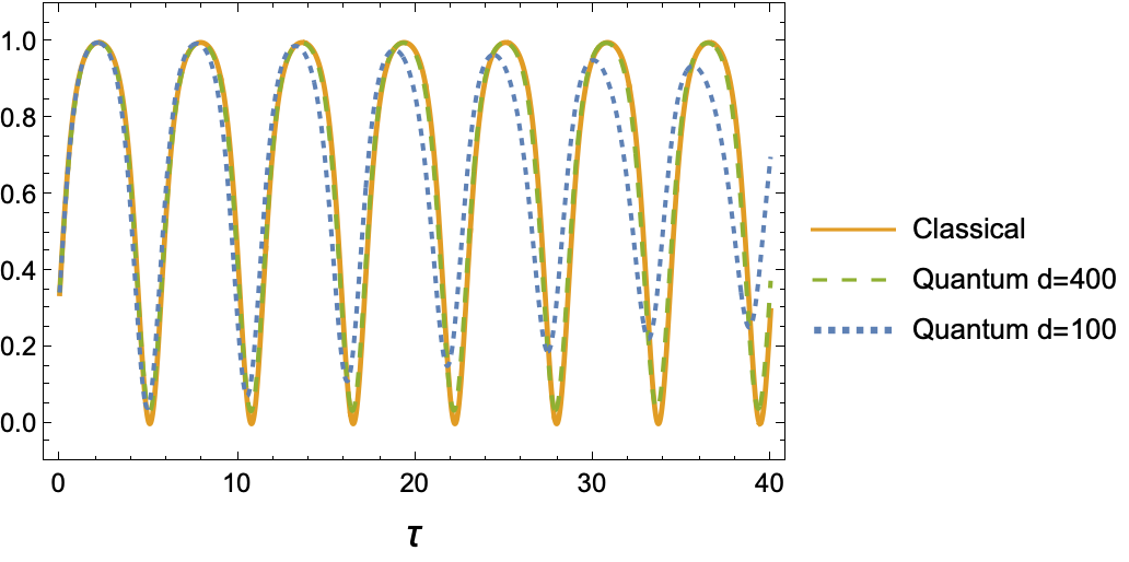
We compare the integrated classical system with initial conditions with the quantum system in Figs. 1, 2, and 7. As discussed above, the initial condition is Gaussian in , and we have also taken , , and the normalization chosen such that the total probability is 1. In what remains of this section, we will consider the quantum-classical correspondence and various effects on that correspondence due to different choices of nonlinearity parameter , the initial standard deviation , and the quantum dimension .
In Fig. 1, we compare three systems, two quantum with and and the classical system, for a nonlinearity parameter . Recall that , and as , the nonlinearity increases. Despite the quantum and classical velocities being independently maximized, there is excellent initial correspondence between all three systems. The nonlinearity is pronounced enough that the system diverges from the classical solution within a couple of periods; however, the correspondence for the system lasts much longer, with the quantum systems accurately capturing both the nonlinearity of the classical orbit as well as its period.
(a)
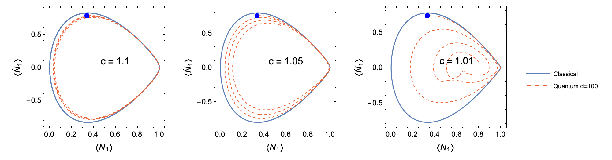
We may more carefully explore the effect of the nonlinearity parameter on the quantum-classical dynamics via phase-space diagrams of the quantum and classical systems in Fig. 2. Three classical nonlinear orbits are shown for each of the nonlinearity parameters , , and . Decreasing the nonlinearity parameter causes the classical orbits to become more pinched. This increasingly linear relationship between and indicates exponential-like growth, the onset of the classical instability and its quantum counterpart (see [26]). From the quantum orbits in Fig. 2, it is obvious that as the nonlinearity increases, the correspondence between the systems decreases. Investigations into exponential growth of quantum correlators in non-chaotic systems indicate that proximity to the classical fixed point leads to quantum scrambling [30]. For instance, after a single pass near the classical fixed point, the system sharply diverges from the classical solution for . On the other hand, the quantum system approximates the classical solution for a couple of classical periods for (see also Fig. 1), and the correspondence lasts for much longer for . The proximate cause of the sharp divergence of the quantum system from the classical system near the fixed point is the increased classical period as . Since the quantum system may only approximate the classical system for finite times, when and the classical period tends to infinity, the quantum solution will inevitably diverge from the classical within a single period.
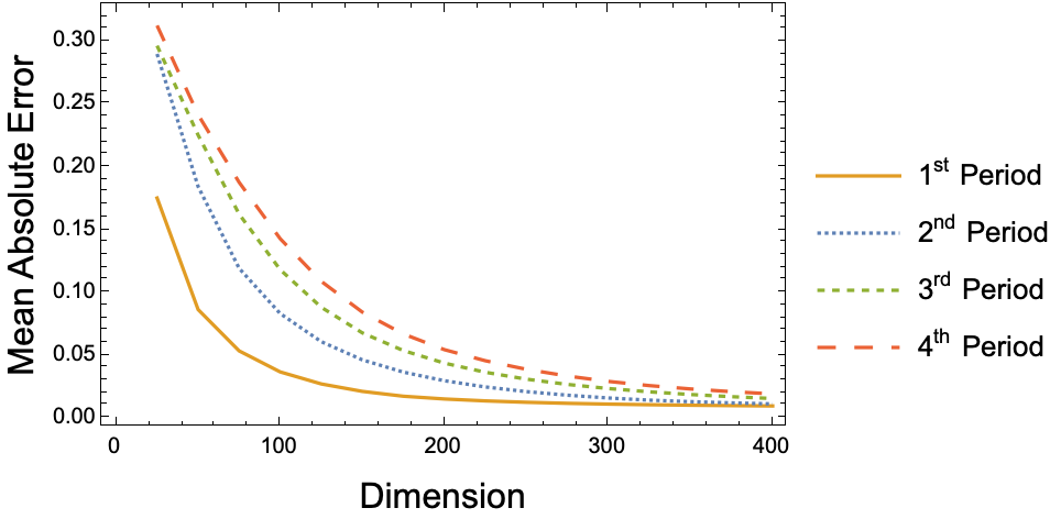
Shown in Fig. 3 is the mean absolute error between the classical system and quantum systems with a range of dimensions and nonlinearity parameter . The error is averaged over one period of the classical orbit for each of the first four classical periods. Note that for two uncorrelated oscillators with amplitude 1, the expected value of the mean absolute error will be 0.25. A mean absolute error higher than this must be due to anti-correlated phases. This occurs for low dimension in Fig. 3. As the dimension of the quantum simulation is increased, the error decays quickly; doubling the dimension of the quantum system more than halves the mean absolute error.
So far, the initial standard deviation of the quantum system has been taken to be for simplicity; however, this does not necessarily lead to the best correspondence with the classical system. There is a trade off between long-term fidelity and the size of the initial variance. Shown in Fig. 4 is the growth of the variance over time given different initial variances. Only the maximum variance is plotted because the magnitude of the variance oscillates with the amplitude of the wave. This can be seen in the spurts of growth of the maximum variance occurring at multiples of the period of the nonlinear oscillation. For a higher initial standard deviation, the variance grows more slowly with time.
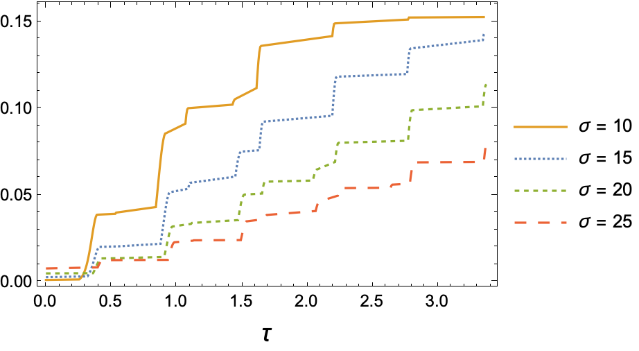
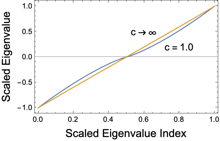
The slow growth of the variance with larger initial standard deviations is attributable to the spectrum of the Hamiltonian, shown in Fig. 4. When , the eigenvalues will be exactly linearly distributed, and for finite , they will lie between the two lines of the figure. Importantly, even for the maximally nonlinear , the eigenvalues with small absolute value (those with scale eigenvalue indices of around ) will still be approximately linearly distributed. As the three-wave interaction acts similarly to a perturbed quantum harmonic oscillator, we may by analogy understand that states with a large initial standard deviation are represented by the lowest energy eigenmodes—those eigenmodes which reside in the central, linear area of Fig. 4. With higher initial variance states having their dominant eigenfrequencies linearly distributed, they remain in correspondence with the classical dynamics for longer periods of time. Thus, despite a high initial variance coming at the cost of the quantum Eq. (32) beginning with dynamics farther from those of the classical Eq. (8) with no variance, the effect of quantum interference is suppressed. Of course, if the initial variance is taken to be too large, 1) the initial condition may no longer be taken to be Gaussian, and 2) the initial condition ceases to be well-approximated by lower frequency eigenstates. An initial standard deviation of strikes a balance between the need for a small growth rate of the variance with the need to prevent clipping of the initial Gaussian in the finite domain with enforced.
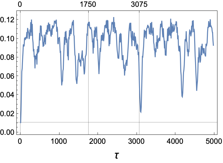
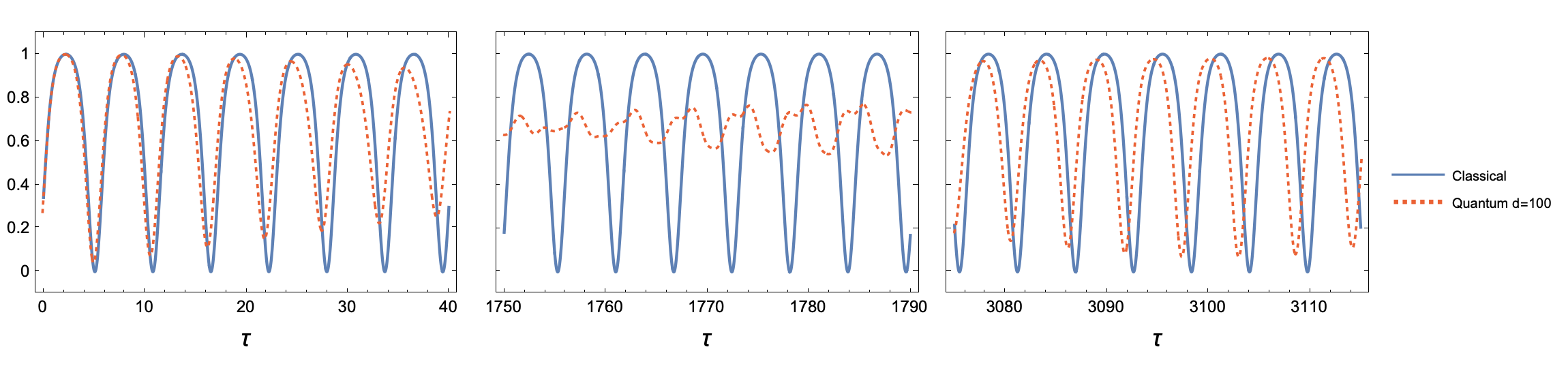
The variance may be used as a tool to determine where quantum revivals will occur. Shown in Fig. 6 is the variance for the quantum system for the first approximately 880 classical orbits. The initial standard deviation is , which corresponds to an initial variance of . Beginning around , the variance sharply decreases to a minimum of indicating a partial quantum revival, shown in Fig. 7. Although the phase and amplitude of the quantum system differ from that of the classical, during the revival, the quantum system accurately captures the period of the classical orbit. When the variance is higher, for example, beginning at , it is difficult to characterize the correlation between the quantum and classical systems.
IV Conclusions
As a model for the classical system, the quantum description of the three-wave interaction has several advantages. First, via the correspondence principle, the classical and quantum systems are guaranteed to converge as the dimension of the quantum system is increased. Second, we did not need to rely on closures or arbitrary choices of a finite representation, as would have been the case for a KvN quantization of the classical dynamics. The quantum field-theoretic method for quantization provides a systematic means of rendering the dynamics discrete, finite-dimensional, and unitary. Finally, as displayed in Figs. 1 and 3, the quantum system of appropriate dimension can capture both the qualitative and quantitative aspects of the nonlinear periodic solution, including its frequency.
While the dimension of the quantum systems being compared to classical dynamics have been large (), simulations of this degree may soon be achievable with quantum computers. Since , where is the number of qubits necessary to represent a state, neglecting error correction, a quantum state only requires 8 qubits to represent it. However, difficulties would arise from approximating the three-wave Hamiltonian as a series of universal gates acting on those qubits. In general, approximating arbitrary unitary operators can require gate applications, which is obviously untenable for high dimension. Shi et al., in simulations of the quantum three-wave equations with , have shown this problem may be sidestepped, though, through the creation of special-made gates particular to the system one is simulating [23].
Another hurdle to quantum simulation of the three-wave interaction relates to the information being extracted from the quantum system. Measuring the full time history of each component of the quantum phase space, , will destroy any potential quantum speedup; however, when compared with simulating the full classical Liouville dynamics, simulating the quantum dynamics may result in speedups as long as the extracted information is sparse. In particular, we have shown that low-dimensional classical information, including the nonlinear frequency and the expectation value of the number operator, may be effectively simulated in a quantum system. While the three-wave interaction is only the lowest order nonlinearity in plasma physics, this opens the possibility of using natively unitary quantum dynamics to model more complicated classical, nonlinear dynamics on quantum hardware in the near future.
Acknowledgements.
This research was supported by the U.S. Department of Energy (DE-AC02-09CH11466).References
- Moody et al. [2012] J. Moody, P. Michel, L. Divol, R. Berger, E. Bond, D. Bradley, D. Callahan, E. Dewald, S. Dixit, M. Edwards, and et al., Nat. Phys. 8, 10.1038/nphys2239 (2012).
- Myatt et al. [2014] J. Myatt, J. Zhang, R. Short, A. Maximov, W. Seka, D. Froula, D. Edgell, and et al., Phys. Plasmas 21, 055501 (2014).
- Zakharov et al. [2012] V. Zakharov, V. L’vov, and G. Falkovich, Kolmogorov Spectra of Turbulence I: Wave Turbulence (Springer, New York, 2012).
- Frantz and Nodvik [1963] L. Frantz and J. Nodvik, J. Appl. Phys. 34, 10.1063/1.1702744 (1963).
- Ahn et al. [2003] J. Ahn, A. Efimov, R. Averitt, and A. Taylor, Opt. Express 11, 10.1364/OE.11.002486 (2003).
- Brunton et al. [2012] G. Brunton, G. Erbert, D. Browning, and E. Tse, Fusion Eng. Des. 87, 10.1016/j.fusengdes.2012.09.019 (2012).
- Kadri and Stiassnie [2013] U. Kadri and M. Stiassnie, J. Fluid Mech. 735, R6 (2013).
- Rosenbluth et al. [1973] M. Rosenbluth, R. White, and C. Liu, Phys. Rev. Lett. 31, 1190 (1973).
- Zakharov and Manakov [1976] V. Zakharov and S. Manakov, Sov. Phys. JETP 42 (1976).
- Kaup et al. [1979] D. J. Kaup, A. Reiman, and A. Bers, Reviews of Modern Physics 51, 275 (1979).
- Reiman [1979] A. Reiman, Reviews of Modern Physics 51, 311 (1979).
- Armstrong et al. [1962] J. A. Armstrong, N. Bloembergen, J. Ducuing, and P. S. Pershan, Phys. Rev. 127, 10.1103/PhysRev.127.1918 (1962).
- Koopman [1931] B. O. Koopman, Proc. Nat. Acad. Sci. 17, 315 (1931).
- v. Neumann [1932] J. v. Neumann, Annals of Mathematics 33, 587 (1932).
- Lan and Mezić [2013] Y. Lan and I. Mezić, Physica D: Nonlinear Phenomena 242, 42 (2013).
- Joseph [2020] I. Joseph, Phys. Rev. Research 2, 043102 (2020).
- Brunton et al. [2016] S. L. Brunton, B. W. Brunton, J. L. Proctor, and J. N. Kutz, PLOS One 11, e0150171 (2016).
- I and S. [1999] M. I and W. S., Chaos 9, 213 (1999).
- M and I [2012] B. M and M. I, Physica D: Nonlinear Phenomena 241, 1255 (2012).
- Shi et al. [2017] Y. Shi, H. Qin, and N. J. Fisch, Physical Review E 96, 023204 (2017).
- Shi [2018] Y. Shi, Plasma Physics in Strong Field Regimes, Ph.D. thesis, Princeton University (2018).
- Shi et al. [2021a] Y. Shi, H. Qin, and N. J. Fisch, Physics of Plasmas 28, 042104 (2021a).
- Shi et al. [2021b] Y. Shi, A. R. Castelli, X. Wu, I. Joseph, V. Geyko, F. Graziani, S. B. Libby, J. B. Parker, Y. J. Rosen, L. A. Martinez, and J. L. DuBois, Phys. Rev. A 103, 062608 (2021b).
- Benenti et al. [2001] G. Benenti, G. Casati, S. Montangero, and D. L. Shepelyansky, Phys. Rev. Lett. 87, 227901 (2001).
- Benenti et al. [2003] G. Benenti, G. Casati, and S. Montangero, Experimental aspects of quantum computing (Springer, New York, 2003) Chap. Quantum Computing and Information Extraction for Dynamical Quantum Systems, pp. 273–293.
- May and Qin [2023a] M. May and H. Qin, Phys. Rev. A 107, 10.1103/PhysRevA.107.062204 (2023a).
- Jurkus and Robson [1960] A. Jurkus and P. N. Robson, Saturation effects in a travelling-wave parametric amplifier, Vol. 107 (Proceings of the IEE-Part B: Electronic and Communication Engineering, 1960).
- Jaynes and Cummings [1963] E. T. Jaynes and F. W. Cummings, Comparison of quantum and semiclassical radiation theories with application to the beam maser, Vol. 51 (Proceedings of the IEEE, 1963).
- May and Qin [2023b] M. May and H. Qin, Algebraic discrete quantum harmonic oscillator with dynamic resolution scaling, ArXiv preprint (2023b).
- Xu et al. [2020] T. Xu, T. Scaffidi, and X. Cao, Phys. Rev. Lett. 124, 140602 (2020).