Discretisation of an Oldroyd-B viscoelastic fluid flow using a Lie derivative formulation
Abstract
In this article we present a numerical method for the Stokes flow of an Oldroyd-B fluid. The viscoelastic stress evolves according to a constitutive law formulated in terms of the upper convected time derivative. A finite difference method is used to discretise along fluid trajectories to approximate the advection and deformation terms of the upper convected derivative in a simple, cheap and cohesive manner, as well as ensuring that the discrete conformation tensor is positive definite. A full implementation with coupling to the fluid flow is presented, along with detailed discussion of the issues that arise with such schemes. We demonstrate the performance of this method with detailed numerical experiments in a lid-driven cavity setup. Numerical results are benchmarked against published data, and the method is shown to perform well in this challenging case.
1 Introduction
Viscoelastic fluids produce a number of phenomena distinct from the familiar behaviour of Newtonian fluids. A broad class of such fluids is that of polymer solutions, for which these phenomena are the result of long chain molecules in the fluid that are large enough to have a meaningful effect on the fluid flow. Such fluids are found in industry in the form of molten plastics or machine lubricants, as well as several biological fluids such as blood. Polymeric fluids are modelled by augmenting the usual fluid flow equations for conservation of mass and momentum with a constitutive law for the polymeric stress, which results in a system of either partial differential or integro-differential equations. This article will focus on the former, with the constitutive law given by a hyperbolic partial differential equation (PDE).
In Newtonian fluid dynamics, the Reynolds number indicates the relative scaling of inertial terms to viscous terms in the Navier-Stokes equations, and can be used to predict flow behaviour and transition between different regimes such as laminar and turbulent flow. In viscoelastic flows, there are two dimensionless groups which are used to predict flow behaviour, the Weissenberg number, and the Deborah number, . The Weissenberg number quantifies the effect of nonlinearities that arise due to non-Newtonian normal stress differences [11, 33]. The Deborah number has been interpreted as the ratio of the magnitudes of elastic and viscous forces [4]. In the limit as , Newtonian flow behaviour is recovered. Experimental results for dilute polymer solutions reported in [32] suggest that a transition to turbulent flow behaviour may occur when elastic effects become dominant over viscous, an effect known as elastic instability, even for small Reynolds number. In complex flow geometries and time-dependent flows, it may be difficult to define these dimensionless groups appropriately, and indeed one may be more relevant than the other. However, in keeping with much of the literature on numerical methods for non-Newtonian flows, we will mainly consider the Weissenberg number , defined as
where is the relaxation time and and are characteristic velocity and length scales of the problem.
Numerical methods posed for the solution of viscoelastic fluid problems, especially using the Oldroyd-B model, have been observed to suffer from the so-called high Weissenberg number problem, where numerical simulations fail to converge at moderate values of the Weissenberg number. There are several potential causes of the high Weissenberg number problem such as the fact that many viscoelastic fluid flow problems exhibit strong, spatially exponential layers which require fine mesh resolution to adequately resolve. In [34], the authors observe a relationship between the Weissenberg number and the principle eigenvalue, determined by numerical simulation and curve fitting. They find that this maximum value increases exponentially with respect to . It is therefore a significant computational cost to resolve this layer for larger Weissenberg number. It has also been suggested that the Oldroyd-B model itself is insufficient to properly describe viscoelastic behaviour. Indeed, extensional viscosity of the Oldroyd-B model blows up at a finite strain rate [21]. Despite this, the Oldroyd-B model remains a popular test case for numerical modelling. This point is discussed in greater detail in §2.
It is also well known that for the Oldroyd-B model, if the initial data for the conformation tensor is positive definite, then the conformation tensor remains so for all time [13, 40]. Loss of positive definiteness at the discrete level is often a precursor to numerical blowup, and indeed it was shown in [42] that the Upper-convected Maxwell model (which is the model that results if the solvent contribution is neglected in the Oldroyd-B model) becomes ill-posed. It therefore appears that designing schemes which preserve the positive definiteness of the discrete conformation tensor is important not only to maintain the physical structures of the model, but also crucial for numerical stability.
These phenomena motivated what seems to be the dominant method for solving viscoelastic constitutive laws in differential form: the log-conformation representation, introduced in [15]. In this approach, a differential equation is derived for the tensor logarithm of the (positive definite) conformation tensor, thus guaranteeing that the numerical approximation to the conformation tensor will remain positive definite. It is argued that this method is more appropriate for resolving exponential spatial layers, and indeed has provided numerical simulations with relatively large Weissenberg numbers [16, 23] which are stable, though questions of accuracy remain. It is however suggested by the results of [45] that careful application of the method is required to preserve physical characteristics of the model. In particular, they report reduced turbulent drag reduction. In addition, solving for the logarithm of the conformation tensor introduces additional nonlinearities into the numerical model that are not present in the physical model, increasing computational expense. Other schemes which preserve positivity have been derived using for example the square root of the conformation tensor [28] and the use of the hyperbolic tangent transformation [24].
Schemes based on a Lie derivative formulation offer a potential solution to the issues described above. While characteristic schemes are motivated by the idea of discretising the material derivative as a single object after expressing it as a rate along fluid trajectories, the upper-convected derivative is similarly expressible as a rate along fluid paths, this time including information on deformation of the moving fluid. Indeed, when expressed in a convected coordinate system, the Oldroyd-B constitutive law is a tensor-valued ordinary differential equation. The method presented in this work can be thought of as resulting from an approximation of a rate of change of stress that also incorporates rate of change of the convected coordinate system used to express it. Discretising the Oldroyd-B constitutive law with an appropriately chosen finite difference methods provides a natural way to preserve positive definiteness of the conformation tensor. To our knowledge, the idea of conducting computations for viscoelastic fluids by discretising the upper convected derivative expressed as a Lie derivative was first proposed in [35]. Theory was developed in [25, 26] for a finite element method in the framework of Ricatti equations. A finite difference scheme for the Oldroyd-B constitutive law with prescribed velocity field was presented with truncation analysis in [30]. These methods can be viewed as an extension of characteristic schemes, which are well established in fluid dynamics due to their favourable stability properties, see [37] for an early reference, with analysis of a finite element method given in [44]. For example, when applied to the transport equation, stable solutions are obtained even for large CFL numbers. These methods have also been used to discretise the advective part of the upper convected derivative in computations involving viscoelastic fluids [8].
The discretisation of this problem in the Lie derivative framework has distinct advantages and unique challenges. One of the goals of the paper is to compare these features with other common approaches, and to test the limits of Lie derivative discretisation methods. We present a scheme based upon the Lie derivative where the conformation tensor is evolved pointwise, and spatial discretisation enters only through the approximation of the deformation gradient tensor and particle trajectories and interpolation. We note that similar schemes have appeared in the literature [3, 25, 26, 30], but our aim in this work is to present results from a full implementation in a challenging test case that can be compared with other published data.
In this article, we provide an accessible overview of viscoelastic fluid dynamics, particularly focused on polymer solutions modeled by the Oldroyd-B constitutive law. We develop a numerically tractable scheme for the model and prove the well-posedness. Our developed scheme also performs favorably in comparison to more computationally intensive alternatives that typically require high performance computing to realise. A thorough comparative study is presented, demonstrating the robustness of our approach. Furthermore, we discuss appropriate mesh design critical for capturing the complex dynamics of viscoelastic flows. This article will focus on the lid-driven cavity problem: a challenging test problem for non-Newtonian flows due to strong shearing that occurs near the moving lid, as well as strong stress gradients at the corners. It is a well-studied benchmark test case in the numerical literature on simulation of the Oldroyd-B model [7, 10, 16, 19, 34, 43], and serves as a useful example to illustrate key differences between Newtonian and non-Newtonian flows.
The outline of the rest of the article is as follows. In §2, we describe the Oldroyd-B model. Key concepts from continuum mechanics are introduced in §3, where a reformulation of the upper convected time derivative is described. In §4, a semidiscrete upper convected time derivative is introduced, and its consistency and approximation order is given. We discuss fully discrete numerical methods in §5. We work with a decoupled formulation, and so we discuss solution of the Stokes and Oldroyd-B systems separately. Descriptions of computational aspects and implementation details, as well as numerical experiments are presented in §6.
2 The Oldroyd-B model
Let be a convex domain with polygonal boundary, and let be the spatial velocity field, with the pressure. The (symmetric) conformation tensor describes the non-Newtonian component of the stress. We let be the rate of strain tensor, or symmetrised velocity gradient:
The Oldroyd-B model for the flow of a fluid in consists of the Navier-Stokes equations for incompressible flow given by
| (1) |
This is coupled to a hyperbolic constitutive law for the evolution of the stress, and is given below in non-dimensional form.
| (2) |
The system has three parameters, namely the familiar Reynolds number , the elasticity ratio and the Weissenberg number, . The regime of interest in this work is low and high . We will assume that to avoid the complications that can arise from the viscous term being removed and the system becoming fully hyperbolic (these difficulties are discussed in more detail in [6]). We note that the conformation tensor is related to the polymeric extra-stress tensor by
We note that in the context in this work (i.e. a lid-driven cavity), the Weissenberg and Deborah numbers are related to each other via the aspect ratio of the cavity [33], and are in fact equal for a cavity of square cross-section.
We prescribe Dirichlet boundary conditions on for the velocity such that on , where is the outward facing normal vector to the boundary, i.e. the problem is driven by tangential boundary values for the velocity. We note that since Dirichlet boundary conditions are prescribed on the whole boundary, to ensure that there exists a uniquely determined pressure field we include the constraint that the pressure has mean zero. Initial conditions for the fluid velocity and conformation tensor are given by and respectively.
The left hand side of Equation (2) is the upper convected time derivative, introduced by Oldroyd [31] and discussed in greater detail in §3. See also [21] for an overview. It gives the rate of change of a tensor quantity in a convected coordinate system which moves and deforms with the fluid. Such a rate is appropriate to derive constitutive laws which exhibit material frame indifference that is, the principle that the physics of the constitutive law should be independent of the frame of the observer.
Remark 2.1 (Boundary conditions for the conformation tensor).
The problem described above is an enclosed flow. Since there is no inflow boundary, and since the constitutive relation (2) is hyperbolic, no boundary condition is required for the conformation tensor. The case of inflow boundary conditions for the velocity, which we do not consider here, requires additional boundary conditions for the conformation tensor. This is not a well studied problem and another potential source of instabilities in these flows.
To complete the exposition, it is appropriate to discuss some of the assumptions made in the derivation of the Oldroyd-B model. The introduction of the upper convected time derivative by Oldroyd [31] assumes that the physics of the constitutive relation are formulated in terms of the evolution of contravariant components of a second order tensor in the convected frame moving and deforming with the fluid. This is a choice, justified by experiments exhibiting rod-climbing (a phenomenon that the Oldroyd-B model replicates), rather than physics, and other choices may be more appropriate (see the discussion in [21]).
The model has also been derived from kinetics using a dumbbell and spring model in which no limit is placed upon the extension of the spring. However, if the flow is strong (that is, if the largest eigenvalue of exceeds , where is the relaxation time [21]), the molecule length increases without limit. It has been shown that, as a result of this, infinite stress can occur in the interior of a steady flow. In many regimes however, the Oldroyd-B fluid is a good approximation of a Boger fluid. It is the simplest differential viscoelastic model available which enjoys material frame indifference (simpler models do exist such as the linear Maxwell model, see [39, Chapter 2] for an overview, but do not have this property). It is also popular, with a wide range of benchmark numerical data available in the literature. It therefore represents a prototypical model for the derivation and testing of numerical methods, see for example [16, 24, 26, 29, 36] and many others.
Remark 2.2.
Taking the kinetic viewpoint, the Oldroyd-B model can be improved by considering for example variants of the Finitely Extensible Nonlinear Elastic (FENE) model for the spring force in the polymer molecules, which limits molecules to be finitely extensible and avoiding the issue of unbounded stress growth. This does however result in a more complicated nonlinearity in the constitutive law. For example, the FENE-P model has constitutive law given by
where the additional parameter represents the maximum extensibility of the polymer molecules. The extension of the current work to more realistic models will be the subject of further research.
3 A Lie derivative framework for the upper convected time derivative
In his seminal paper [31], Oldroyd described the importance of formulating a time derivative with which to construct constitutive laws for non-Newtonian stresses that does not depend on the choice of reference frame. Such derivatives have to take account of the moving fluid flow and its deformation. The upper convected time derivative, one of two derivatives introduced by Oldroyd, is one of (infinitely) many such time derivatives. It is now well known that these rates are special cases of Lie derivatives (see eg [22, chapter II]), and formulating the constitutive law in a way that respects this can have structure-preserving advantages. In this section we give the concepts necessary to formulate the constitutive law for a non-Newtonian fluid as a Lie derivative.
3.1 Flow map and deformation gradient
Let be the flow map for the fluid motion. That is, the fluid particle which at time has position has position at time . The flow map satisfies the following ordinary differential equation
One can express the material derivative in terms of the flow map by examining the infinitesimal derivative, that is
We define the velocity gradient with the convention that it has components
and make note that some authors define the velocity gradient as the transpose of the above tensor. The deformation gradient tensor describes the deformation experienced by a fluid parcel in a neighbourhood of between times and . In a Cartesian coordinate system, it has components
| (3) |
It can alternatively be expressed in the following way:
Where no confusion can occur, we will omit the particle label and for brevity write for and for .
It follows immediately from the definition that , where is the identity tensor, and that . The deformation gradient is a two point tensor, and the following lemma describes its evolution with respect to the two faux time indices:
Lemma 3.1 (Evolution of the deformation gradient along characteristics).
The deformation gradient tensor satisfies the following differential equations.
| (4) |
| (5) |
Proof.
Proposition 3.2.
3.2 The upper convected time derivative
For a generic sufficiently smooth tensor function , the upper convected derivative is defined through
This has a relationship to the notion of a Lie derivative of the tensor quantity which we will exploit in this work. Indeed, one may introduce the Lie derivative which follows the fluid with deformation gradient tensor by
The upper-convected derivative can be inferred from the fundamental properties of given in §3.1 [25, 30]
The Oldroyd-B constitutive relation for the conformation tensor can therefore be formulated in terms of the Lie derivative resulting in an equation in one (characteristic) time variable as follows
| (6) |
We see that the constitutive law in Oldroyd-B is a linear ODE along the characteristics induced by the deformation gradient . This is why Oldroyd-B is often referred to as a linear viscoelastic model. It also offers the opportunity to utilise the a wide variety of timestepping methods designed for problems of this kind.
4 Discretisation of the upper convected time derivative
In this section we introduce a discretisation of the upper convected time derivative motivated by its formulation as a Lie derivative given in §3. The method will be similar to characteristic schemes, where the material derivative is discretised along the characteristics of the flow [37, 41, 44]. Adapting this methodology to account for the deformation of the fluid provides a natural way to preserve the positive definiteness of the conformation tensor of any given discretisation. This idea has been explored previously in the context of several different numerical frameworks [8, 26, 30, 35].
We divide the time domain into a uniform partition of subintervals of length (so that ). We write for , non uniform timestepping is certainly possible however for clarity of exposition we will restrict to uniform. We also use the notation . Starting from
| (7) |
we will utilise a finite difference approach which motivates the following definitions:
Definition 4.1 (Semidiscrete upper convected derivative).
For , and , define
| (8) |
as an approximation of the departure point of under the fluid velocity at time . Further, let
| (9) |
denote an approximation of the deformation gradient tensor between times and . We define a discrete upper-convected time derivative of a generic, sufficiently smooth, tensor function by the velocity field as
Remark 4.2.
Different choices are available to make this approximation depending on the desired properties of the scheme. Definition 4.1 results from choosing a backward Euler discretisation, whereby the right hand side of Equation (7) is approximated by
which after evaluating at becomes
| (10) |
It is not always practical (or possible) to exactly evaluate the deformation gradient and flow map, so they are replaced with approximations and respectively in the definition of .
The structure associated to (6) is dissipative in nature hence a BDF discretisation is quite natural. A detailed discussion of approximations of the upper convected time derivative in the manner described above is given in [30], where the authors discuss first and second order approximations of BDF type.
We now turn our attention to well-posedness and properties of the scheme. We first show in Lemma 4.3 that is well-defined as long as is chosen to be sufficiently small. For a velocity satisfying a homogeneous Dirichlet boundary condition, this result is proved in [41]. We provide an extension of that result appropriate for nonzero tangential velocity boundary conditions such as the lid-driven cavity.
Lemma 4.3.
Let be the unit square or the unit cube. Assume that on , and that is chosen so that . Then for any , and any , we have .
Proof.
Let . Then, by (8)
The boundary of has the form where is a line segment when and a plane segment when . Let and for some , denote by the unique point on that satisfies . As is convex this point clearly lies in the interior of , so that the unit outward normal to the boundary at is well-defined, and the line segment joining and is perpendicular to . We consider the component of the velocity in the direction of . Since ,
where is the unit normal to at . Again, using (8) we have shown that
that is, the velocity at in the direction of is not large enough for the line segment joining and to cross . Since the choice of was arbitrary, we must have that . ∎
In the following lemmata, we discuss the approximation properties of , and finally . We will utilise certain results which were proved in [30]. The first, Lemma 4.4, gives a bound on the error arising from approximating the departure point using (8) (see Figure 1 for an illustration), while Lemma 4.5 bounds the error in evaluating a tensor function at this approximate departure point as opposed to the true point. The error in approximating the deformation gradient is bounded in Lemma 4.6, and finally a bound showing the consistency and approximation order of the discrete upper convected derivative is given in Theorem 4.8.
Lemma 4.4 (Approximation of characteristics [30, Lemma 2]).
Suppose that on and
that
. Then for any and ,
| (11) |
Lemma 4.5.
In addition to the hypotheses of Lemma 4.4, let be an appropriately differentiable tensor function. Then for any and ,
Lemma 4.6 (Approximation of deformation gradient [30, Lemma 1]).
Suppose that the hypotheses of Lemma 4.4 are satisfied. Then for any and ,
Remark 4.7.
We finally arrive at the approximation of the upper convected derivative (see [30, Remark 7]).
Theorem 4.8.
Suppose that the hypotheses of Lemma 4.4 are satisfied, and that is an appropriately differentiable tensor function. Then for any and ,
Theorem 4.8 may be interpreted as an expansion around in that if follows directly that we have, at ,
We are now in a position to state the semidiscrete scheme for the constitutive law (2).
4.1 Semidiscretisation of the Oldroyd-B constitutive law
Suppose that is given for and . Suppose also that an initial condition is given. Then for we define by
| (12) |
Proposition 4.9 (Consistency).
The semidiscrete scheme given in (12) is a consistent, first order approximation.
Proof.
By Theorem 4.8, we have the following representation:
Then, using Equation (2), we obtain
| (13) |
Assuming that is given, one step of the semidiscrete scheme gives that satisfies
| (14) |
Finally, noting that for any , we have , so that subtracting (14) from (13) gives
and therefore the semidiscrete scheme has local truncation error proportional to . ∎
Proposition 4.10 (The positive definiteness of the conformation tensor is preserved).
Suppose that
is given, and is positive definite, and assume that is given. Then there exists such that is positive definite.
Proof.
We can write (12) as
| (15) |
Thus, as long as is chosen small enough, a sufficient condition would be for example, is invertible by the Gershgorin circle theorem [18, Thm 7.2.1]. Let . Then since is invertible, the product is a nonzero vector in , so that by hypothesis
Then from (15), is a sum of two positive definite terms. ∎
5 Spatial discretisation
In this section we present numerical methods for the Oldroyd-B fluid in the case . The problem is solved in a decoupled manner, in which at each time step a Stokes problem is solved for the fluid velocity, which is then used as a forcing in the time-dependent constitutive relation. This avoids the need to solve a very large monolithic system and therefore keeps computational costs down. We first give a finite element method to solve the Stokes problem and discuss well-posedness. We then present the fully discrete constitutive law and discuss the solution procedure for the full problem.
5.1 Finite element discretisation for the Stokes problem
We consider to be a conforming triangulation of , namely, is a finite family of sets such that
-
1.
implies is an open box (i.e. a quadrilateral or hexahedron),
-
2.
for any we have that is a full lower-dimensional box (i.e., it is either , a vertex, an edge (or face) or the whole of and ) of both and and
-
3.
.
Further, we define to be the piecewise constant meshsize function of given by
With the space of bilinear polynomials over a quadrilateral (or trilinear over a hexahedron), we introduce the finite element space
to be the usual space of continuous piecewise bilinear functions. Let the vertices of the triangulation be denoted . For a vertex , we define
To facilitate strong imposition of boundary conditions for the velocity, we introduce finite element spaces
To solve the Stokes problem, we employ the stabilised equal-order approximation introduced in [12]. The stabilisation makes use of the projection operator that maps the finite element space to a space of discontinuous functions which are constant on each element. The construction of the stabilisation term is therefore local to elements. In addition, this scheme performs well on graded meshes, which are a useful tool due to the sharp boundary layers that occur in viscoelastic fluid flows (see §6.2). A more detailed discussion and analysis for this scheme can be found in [5, 12, 14]. Let be a given interpolant of . Then the discrete problem for the velocity and pressure is to find such that
| (16) |
for all .
Proposition 5.1 (Inf-sup stability [5]).
Let
| (17) |
Then, there exists a independent of such that
| (18) |
The inf-sup condition guarantees that problem (16) is well-posed.
5.2 A finite difference approximation of the upper convected time derivative
The discretisation of the constitutive law requires several definitions relating to approximations of characteristics and deformation gradients, which we now give. We write for the discrete solution at time .
Remark 5.2.
Definition 5.3.
Let be given. For any and , define the discrete departure point of according to the velocity as
| (19) |
We also define the discrete deformation gradient between time and as
Definition 5.4 (Fully discrete approximate upper convected time derivative).
Let be given, and suppose that are tensor valued functions representing the the value of a time dependent tensor field at the time levels . Then the fully discrete approximation to the upper convected time derivative of at time level is given by
| (20) |
5.3 A fully discrete scheme for the Stokes flow of an Oldroyd-B fluid
We are now in a position to define the full finite difference discretisation of the constitutive law. Values of the discrete conformation tensor are stored at the vertices . At any time level , these values are sufficient to uniquely define a function by bilinear (or trilinear) interpolation. This representation is used to evaluate the conformation tensor at points which are not vertices, and is the function on the right hand side of the discrete Stokes equation (16). By a slight abuse of notation, we will write for both the set of point values at vertices, and the function in obtained by interpolation using these values.
We note that the approximation of the deformation gradient needed to evaluate (20) requires the value of the discrete velocity gradient, which we wish to use at the vertices of the mesh. Since the discrete velocity lies in , the point values of its gradient are not well defined. For a vertex of the mesh and a function , in place of the velocity gradient, we therefore use the local average over :
The fully discrete problem is given as follows. Let be an interpolant of the initial condition. Then for , find , such that
| (21) |
for all , then is given by
| (22) |
At each mesh point, (22) is a coupled system of ordinary differential equations forced by the discrete fluid velocity via the deformation gradient, and approximated in an explicit manner, and therefore the nodal values may be updated without the need to solve a linear system.
Remark 5.5 (Choice of spatial discretisation points for finite difference scheme).
We note that since all derivatives appearing in the constitutive relation are approximated via (10), we are free to choose any set of points at which to approximate the conformation tensor, with the proviso that care must be taken to adequately resolve the velocity gradient, as this is what forces the constitutive law. The choice of these points so that they correspond with the degrees of freedom of a piecewise bilinear finite element space is a natural one, as it is then clear how to include the discrete conformation tensor in the momentum equation. Other possible choices are discussed in §7.
Proposition 5.6.
If the initial condition is positive definite, and bilinear interpolation is used to obtain and to evaluate at points which are not vertices of the mesh, then at each time step there exists such that the discrete conformation tensor remains positive definite.
Proof.
By assumption, all nodal values of are positive definite. Then since interpolated values are weighted sums of the nodal values with non-negative weights, the interpolant is also positive definite. By the same argument as in Proposition 4.10, if we choose , and if is positive definite, then computed from the scheme (22) will also be positive definite. ∎
6 Numerical Experiments
In this section, we present numerical results obtained by solving (21)-(22) for a variety of model and discretisation parameters. All simulations presented here were conducted using deal.II, an open source C++ software library providing tools for finite element computations [2].
6.1 Description of the test case
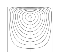
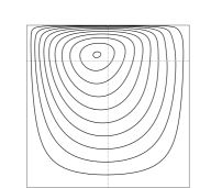
The lid-driven cavity consists of a fluid-filled, impenetrable box in which the flow is driven by a moving lid. The flow of a Newtonian fluid in a lid-driven cavity is by now a very well studied problem. It is known that the flow characteristics, see Figure 2, depend upon the Reynolds number. Studies from the numerical literature largely agree with one another qualitatively and quantitatively for moderate Reynolds numbers. For larger Reynolds numbers, numerical solutions become more challenging, and differences appear in computational results. Detailed numerical studies have provided benchmarks for Reynolds numbers in the tens of thousands [9, 17].
In experimental studies, for small Reynolds number, flow in the cavity reaches a steady state, and, in a three dimensional cavity, remains approximately two dimensional. For the setup in Figure 2, i.e., with lid moving left to right, as the Reynolds number increases the centre of the main vortex moves to the right. Above a critical value of the Reynolds number, the flow transitions to a time-periodic state with variation in the neutral direction [1]. Even for inertialess non-Newtonian flows, the symmetry of the flow is broken (see Figure 2, right) and moves towards the upper left corner with increasing Weissenberg number [33].
In this work, the regularised lid-driven cavity problem was solved, for which , on the lateral and lower boundaries, and on the lid (i.e. ), the velocity boundary condition is
Remark 6.1.
For this problem, a Weissenberg number can be defined as
where is a characteristic relaxation time of the fluid, is a characteristic velocity scale and is the height of the cavity. Thus, is a measure of the shear rate [33]. For the setup described above, , .
6.2 Mesh design
Mesh design and selection of discretisation parameters appears to be of crucial importance for the cavity flow of an Oldroyd-B fluid, and indeed very few studies have reported satisfactory numerical results for the lid-driven cavity using a uniform mesh, with the notable exception of schemes which utilise the log-conformation tensor formulation. In addition, results for some schemes have been shown to be very sensitive to mesh size, for example in [7], dissipation properties, positive definiteness of the conformation tensor and existence of steady state change qualitatively upon varying the mesh size.
For the cavity problem, graded meshes of various types are a common choice. Meshes constructed in this manner are able to provide very fine resolution near the boundary (particularly the lid), where it is most needed, in an efficient manner. The situation may be compared to singularly perturbed convection-diffusion problems, which exhibit boundary layers that put severe limitations on the mesh size. To make computations tractable, layer-adapted meshes have been extensively researched in this community (see [27] for a review). A particularly effective example is the Bakhvalov-type mesh, where upper bounds on the derivatives of the solution near the boundary are used to design mesh grading functions that are sufficient to resolve it.
In this work, we will use a mixture of the following. One construction consists of decreasing element size towards the boundary with a constant contraction ratio , i.e. where the index is such that is the next element in the direction of the boundary [10, 43]. Another is to decrease element size by a constant amount so that [34]. For comparison, the latter is equivalent to decreasing the contraction ratio, so that elements size decreases very rapidly near the boundary. Finally, in [19], mixtures of uniform grid spacing and refined areas are used.


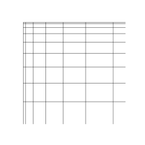

Meshes constructed from central square elements with a constant reduction ratio of 0.96 towards each boundary are denoted by , where is the number of elements in each coordinate direction. We denote by meshes constructed with linearly decreasing element size as follows (similar to those used in [34]). We define vertices for an quadrilateral mesh by their and coordinates, given respectively by for , with for , and for . On these meshes, the finest vertical resolution occurs at the lid, with an element height of .
This means the meshes are highly anisotropic away from the corners. Stabilised finite element methods often have stabilisation parameters that depend badly on the anisotropy of the elements, however the solver we used (16) is parameter free.
| Mesh | # elements | ||
|---|---|---|---|
| 8,100 | 0.0039 | 0.024 | |
| 14,400 | 0.0020 | 0.022 | |
| 22,500 | 0.0010 | 0.021 | |
| 32,400 | 0.00054 | 0.021 | |
| 65,536 |
6.3 Numerical results
Where possible, the results presented here are compared with the literature, particularly [16, 34, 43] - see Table 2. Descriptions of the meshes used are given in §6.2, and a summary of the key statistics of each is given in Table 1. The data for comparison are the logarithm of the maximum value of along the midline, , the maximum value of over the domain, and the coordinates of the centre of the main vortex, .
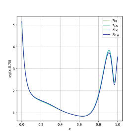
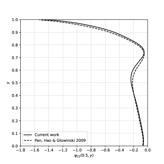
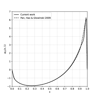
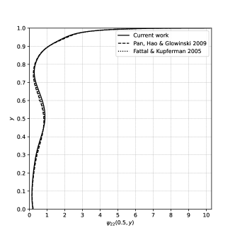
6.3.1
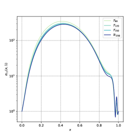
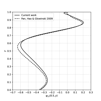
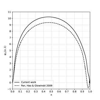
The solution appears to have reached a steady state by . In Figure 4, components of the conformation tensor are plotted along cross sections of the domain for and for various computational meshes described in §6.2 and Table 1. The solutions obtained for and agree qualitatively very well with Figure 5 of [34], albeit with differences in magnitude along the lid. We note that the meshes used there are finer, which could account for the difference. Other metrics available for comparison from the numerical literature (see Table 4 in [43] and Table 2) are the centre of the main vortex in the velocity field and the logarithm of the maximum value of attained along the line . Computed on mesh , the former agrees very closely (within 1%) although not much variation in prediction of this quantity is observed across the numerical literature. The latter is approximately 2% larger than the other predictions given in [43]. Resolution of the layer at the top boundary appears to be of critical importance for the accuracy of the approximation. Under-resolution results in altered behaviour of at the upper boundary. In addition, coarse meshes appear to over-estimate . These errors do not appear to pollute the solution away from the boundary.
| Reference | |||
| Current work | 5.76 | 351.21 | 0.466, 0.799 |
| Current work | 5.65 | 309.65 | 0.466, 0.799 |
| Current work | 5.60 | 295.04 | 0.467, 0.799 |
| Current work | 5.59 | 290.59 | 0.467, 0.799 |
| Pan et al. [34] | 0.469, 0.798 | ||
| Sousa et al. [43] M4 | 5.51 | - | 0.466, 0.800 |
| Current work | 10.75 | 48,038.9 | 0.428, 0.819 |
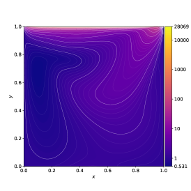
| Current work | 10.22 | 28,069.2 | 0.431, 0.819 |
| Pan et al. [34] | 11,529.43 | 0.439, 0.816 | |
| Sousa et al. [43] M4 | 7.80 | - | 0.434, 0.816 |
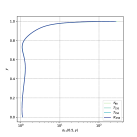
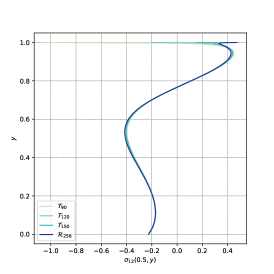
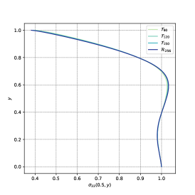
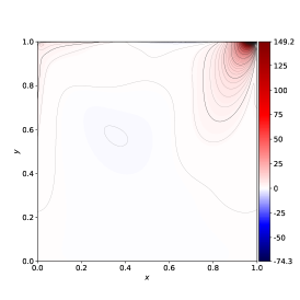
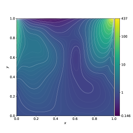
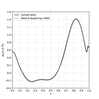
6.3.2
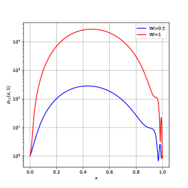
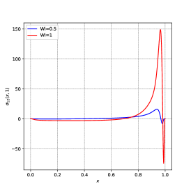
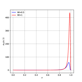
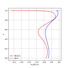
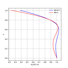
The solution appears to have reached a steady state by . The conformation tensor field is plotted component-wise in Figure 5, with benchmark metrics reported in Table 2. The logarithm of the conformation tensor was computed to allow comparison with other published works, with selected cross sections presented in Figure 6. A sharp boundary layer at the lid is observed in , with all components exhibiting large gradients near the upper corners of the domain. Our computational results agree qualitatively with those presented in [16, Figure 4], although in our simulations a steady state was reached much later than , as reported there. In addition, the maximum value along was significantly overestimated in our work relative to other published data, but there is significant variation in this figure, with [34] reporting a value two logarithmic orders larger than [16]. However, it can be seen from Figure 6 that large discrepancies occur only in a very small neighbourhood of the upper boundary. Qualitative differences are observed only in the upper right hand corner.
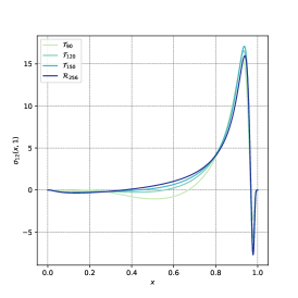
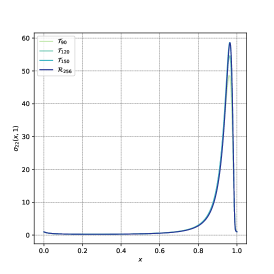
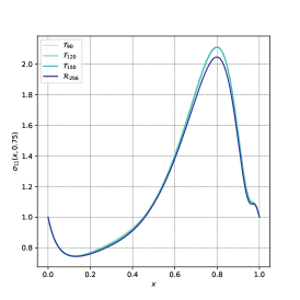
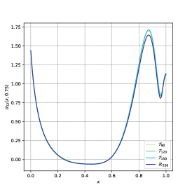
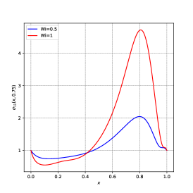
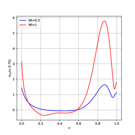
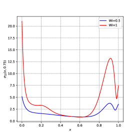
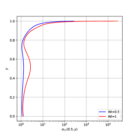
In Figure 7, components of the conformation tensor are plotted along cross sections for two Weissenberg numbers, 0.5 and 1, to illustrate the difference in solutions. Larger magnitudes and exaggerated features are observed in all components for when compared with .
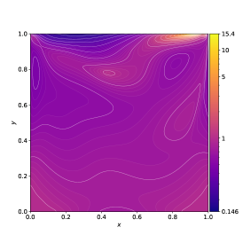
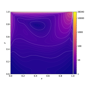
6.4 Positive definiteness of the discrete conformation tensor
A major aim of the numerical scheme presented is to maintain a positive definite comformation tensor, both to respect the physics of the problem and avoid numerical instabilities that can arise when this property is lost. We recall from Proposition 5.6 that this is guaranteed if the time step is chosen to be sufficiently small. To ensure that an appropriate choice was made, the eigenvalues of the discrete conformation tensor were computed, and indeed at all times, the smallest eigenvalue of the conformation tensor was strictly positive, and therefore the discrete conformation tensor remained positive definite throughout the computation. The eigenvalues of the conformation tensor are visualised in Figure 8.
7 Conclusions & Discussion
Results from simulations of an Oldroyd-B fluid in the creeping flow regime using a discretisation of the Lie derivative (7) were presented. The scheme maintained positive definiteness of the discrete conformation tensor and achieved good agreement with existing published data. Our proposed finite difference method circumvents quadrature issues, representing advection effectively compared to some finite element schemes, which can under-represent advection for small time steps or coarse quadrature formulas [8].
Qualitatively and quantitatively, the results are consistent with those in the literature using the log-conformation representation [16, 34, 43]. The scheme’s update process for the conformation tensor is efficient and straightforward to implement. However, spatial resolution and mesh design significantly influence the results, requiring fine meshes for convergence.
Further work includes exploring enhancements to preserve additional fluid structures, particularly incompressibility constraints and investigating differential equations on the special linear group for a consistent discrete deformation gradient. This may involve combining the approach with divergence-free finite element methods for fluid equations or exploring finer meshes or different finite difference points for the constitutive law to address challenges in the creeping flow regime.
8 Acknowledgements
This work has been partially supported by the Leverhulme Trust Research Project Grant No. RPG-2021-238. TP is also partially supported by EPRSC grants EP/W026899/2, EP/X017206/1 and EP/X030067/1. The authors also want to thank Gabriel Barrenechea and Emmanuil Geourgoulis for helpful discussions and suggestions.
References
- [1] Cyrus K Aidun, NG Triantafillopoulos and JD Benson “Global stability of a lid-driven cavity with throughflow: Flow visualization studies” In Physics of Fluids A: Fluid Dynamics 3.9 American Institute of Physics, 1991, pp. 2081–2091
- [2] Daniel Arndt et al. “The deal.II finite element library: Design, features, and insights” In Computers & Mathematics with Applications 81, 2021, pp. 407–422 DOI: 10.1016/j.camwa.2020.02.022
- [3] Mohammed Bensaada, Driss Esselaoui and Pierre Saramito “Error estimate for the characteristic method involving Oldroyd derivative in a tensorial transport problem” In Electronic Journal of Differential Equations, 2004
- [4] Robert Byron Bird, Robert Calvin Armstrong and Ole Hassager “Dynamics of polymeric liquids. Vol. 1: Fluid mechanics” John WileySons Inc., New York, NY, 1987
- [5] Pavel B Bochev, Clark R Dohrmann and Max D Gunzburger “Stabilization of low-order mixed finite elements for the Stokes equations” In SIAM Journal on Numerical Analysis 44.1 SIAM, 2006, pp. 82–101
- [6] J Bonvin, M Picasso and R Stenberg “GLS and EVSS methods for a three-field Stokes problem arising from viscoelastic flows” In Computer Methods in Applied Mechanics and Engineering 190.29-30 Elsevier, 2001, pp. 3893–3914
- [7] Sébastien Boyaval “Lid-driven-cavity simulations of Oldroyd-B models using free-energy-dissipative schemes” In Numerical Mathematics and Advanced Applications 2009: Proceedings of ENUMATH 2009, the 8th European Conference on Numerical Mathematics and Advanced Applications, Uppsala, July 2009, 2010, pp. 191–198 Springer
- [8] Sébastien Boyaval, Tony Lelièvre and Claude Mangoubi “Free-energy-dissipative schemes for the Oldroyd-B model” In ESAIM: Mathematical Modelling and Numerical Analysis 43.3 EDP Sciences, 2009, pp. 523–561
- [9] Charles-Henri Bruneau and Mazen Saad “The 2D lid-driven cavity problem revisited” In Computers & fluids 35.3 Elsevier, 2006, pp. 326–348
- [10] Raphaël Comminal, Jon Spangenberg and Jesper Henri Hattel “Robust simulations of viscoelastic flows at high Weissenberg numbers with the streamfunction/log-conformation formulation” In Journal of Non-Newtonian Fluid Mechanics 223 Elsevier, 2015, pp. 37–61
- [11] JM Dealy “Weissenberg and Deborah numbers—their definition and use” In Rheol. Bull 79.2, 2010, pp. 14–18
- [12] Clark R Dohrmann and Pavel B Bochev “A stabilized finite element method for the Stokes problem based on polynomial pressure projections” In International Journal for Numerical Methods in Fluids 46.2 Wiley Online Library, 2004, pp. 183–201
- [13] F Dupret and JM Marchal “Sur le signe des valeurs propres du tenseur des extra-contraintes dans un écoulement de fluide de Maxwell” In Journal de mécanique théorique et appliquée 5.3, 1986, pp. 403–427
- [14] Howard C Elman, David J Silvester and Andrew J Wathen “Finite elements and fast iterative solvers: with applications in incompressible fluid dynamics” Oxford university press, 2014
- [15] Raanan Fattal and Raz Kupferman “Constitutive laws for the matrix-logarithm of the conformation tensor” In Journal of Non-Newtonian Fluid Mechanics 123.2-3 Elsevier, 2004, pp. 281–285
- [16] Raanan Fattal and Raz Kupferman “Time-dependent simulation of viscoelastic flows at high Weissenberg number using the log-conformation representation” In Journal of Non-Newtonian Fluid Mechanics 126.1 Elsevier, 2005, pp. 23–37
- [17] UKNG Ghia, Kirti N Ghia and CT Shin “High-Re solutions for incompressible flow using the Navier-Stokes equations and a multigrid method” In Journal of computational physics 48.3 Elsevier, 1982, pp. 387–411
- [18] Gene H Golub and Charles F Van Loan “Matrix computations” JHU press, 2013
- [19] Florian Habla, Ming Wei Tan, Johannes Haßlberger and Olaf Hinrichsen “Numerical simulation of the viscoelastic flow in a three-dimensional lid-driven cavity using the log-conformation reformulation in OpenFOAM®” In Journal of Non-Newtonian Fluid Mechanics 212 Elsevier, 2014, pp. 47–62
- [20] Ernst Hairer, Marlis Hochbruck, Arieh Iserles and Christian Lubich “Geometric numerical integration” In Oberwolfach Reports 3.1, 2006, pp. 805–882
- [21] John Hinch and Oliver Harlen “Oldroyd B, and not A?” In Journal of Non-Newtonian Fluid Mechanics 298 Elsevier, 2021, pp. 104668
- [22] Thomas JR Hughes “Numerical implementation of constitutive models: rate-independent deviatoric plasticity” In Theoretical foundation for large-scale computations for nonlinear material behavior: Proceedings of the Workshop on the Theoretical Foundation for Large-Scale Computations of Nonlinear Material Behavior Evanston, Illinois, October 24, 25, and 26, 1983, 1984, pp. 29–63 Springer
- [23] Martien A Hulsen, Raanan Fattal and Raz Kupferman “Flow of viscoelastic fluids past a cylinder at high Weissenberg number: stabilized simulations using matrix logarithms” In Journal of Non-Newtonian Fluid Mechanics 127.1 Elsevier, 2005, pp. 27–39
- [24] Azadeh Jafari, Alireza Chitsaz, Reza Nouri and Timothy N Phillips “Property preserving reformulation of constitutive laws for the conformation tensor” In Theoretical and Computational Fluid Dynamics 32 Springer, 2018, pp. 789–803
- [25] Young-Ju Lee and Jinchao Xu “New formulations, positivity preserving discretizations and stability analysis for non-Newtonian flow models” In Computer methods in applied mechanics and engineering 195.9-12 Elsevier, 2006, pp. 1180–1206
- [26] Young-Ju Lee, Jinchao Xu and Chen-Song Zhang “Stable finite element discretizations for viscoelastic flow models” In Handbook of numerical analysis 16 Elsevier, 2011, pp. 371–432
- [27] Torsten Linß “Layer-adapted meshes for convection–diffusion problems” In Computer Methods in Applied Mechanics and Engineering 192.9-10 Elsevier, 2003, pp. 1061–1105
- [28] Alexei Lozinski and Robert G Owens “An energy estimate for the Oldroyd B model: theory and applications” In Journal of non-newtonian fluid mechanics 112.2-3 Elsevier, 2003, pp. 161–176
- [29] Mária Lukáčová-Medvid’ová, Hirofumi Notsu and Bangwei She “Energy dissipative characteristic schemes for the diffusive Oldroyd-B viscoelastic fluid” In International Journal for Numerical Methods in Fluids 81.9 Wiley Online Library, 2016, pp. 523–557
- [30] Debora D Medeiros, Hirofumi Notsu and Cassio M Oishi “Second-order finite difference approximations of the upper-convected time derivative” In SIAM Journal on Numerical Analysis 59.6 SIAM, 2021, pp. 2955–2988
- [31] James G Oldroyd “On the formulation of rheological equations of state” In Proceedings of the Royal Society of London. Series A. Mathematical and Physical Sciences 200.1063 The Royal Society London, 1950, pp. 523–541
- [32] Peyman Pakdel and Gareth H McKinley “Cavity flows of elastic liquids: purely elastic instabilities” In Physics of Fluids 10.5 American Institute of Physics, 1998, pp. 1058–1070
- [33] Peyman Pakdel, Stephen H Spiegelberg and Gareth H McKinley “Cavity flows of elastic liquids: two-dimensional flows” In Physics of Fluids 9.11 American Institute of Physics, 1997, pp. 3123–3140
- [34] Tsorng-Whay Pan, Jian Hao and Roland Glowinski “On the simulation of a time-dependent cavity flow of an Oldroyd-B fluid” In International Journal for Numerical Methods in Fluids 60.7 Wiley Online Library, 2009, pp. 791–808
- [35] Jerzy Petera “A new finite element scheme using the Lagrangian framework for simulation of viscoelastic fluid flows” In Journal of non-newtonian fluid mechanics 103.1 Elsevier, 2002, pp. 1–43
- [36] F Pimenta and MA Alves “Stabilization of an open-source finite-volume solver for viscoelastic fluid flows” In Journal of Non-Newtonian Fluid Mechanics 239 Elsevier, 2017, pp. 85–104
- [37] Olivier Pironneau “On the transport-diffusion algorithm and its applications to the Navier-Stokes equations” In Numerische Mathematik 38 Springer, 1982, pp. 309–332
- [38] “PlotDigitizer: Version 3.1.5”, 2023 URL: https://plotdigitizer.com
- [39] Michael Renardy “Mathematical analysis of viscoelastic flows” SIAM, 2000
- [40] Michael Renardy and Becca Thomases “A mathematician’s perspective on the Oldroyd B model: Progress and future challenges” In Journal of Non-Newtonian Fluid Mechanics 293 Elsevier, 2021, pp. 104573
- [41] Hongxing Rui and Masahisa Tabata “A second order characteristic finite element scheme for convection-diffusion problems” In Numerische Mathematik 92.1 Springer, 2002, pp. 161–177
- [42] IM Rutkevich “The propagation of small perturbations in a viscoelastic fluid” In Journal of Applied Mathematics and Mechanics 34.1 Elsevier, 1970, pp. 35–50
- [43] RG Sousa, RJ Poole, AM Afonso, FT Pinho, PJ Oliveira, A Morozov and MA Alves “Lid-driven cavity flow of viscoelastic liquids” In Journal of Non-Newtonian Fluid Mechanics 234 Elsevier, 2016, pp. 129–138
- [44] Endre Süli “Convergence and nonlinear stability of the Lagrange-Galerkin method for the Navier-Stokes equations” In Numerische Mathematik 53 Springer, 1988, pp. 459–483
- [45] Wen-Hua Zhang, Jingfa Li, Qiankun Wang, Yu Ma, Hong-Na Zhang, Bo Yu and Fengchen Li “Comparative study on numerical performances of log-conformation representation and standard conformation representation in the simulation of viscoelastic fluid turbulent drag-reducing channel flow” In Physics of Fluids 33.2 AIP Publishing, 2021