From black hole mimickers to black holes

Abstract

We present a simple analytical model for studying the collapse of an ultracompact stellar object (regular black hole mimicker with infinite redshift surface) to form a (integrable) black hole, in the framework of General Relativity. Both initial and final configurations have the same ADM mass, so that the transition represents an internal redistribution of matter without emission of energy. The model, despite being quite idealized, can be viewed as a good starting point to investigate near-horizon quantum physics.

I Introduction

Ultracompact stellar objects are matter distributions with radii ever so slightly larger than their gravitational (Schwarzschild) radius. Therefore their luminosity is subjected to a very large (perhaps even infinite) redshift and they turn out to be excellent candidates for black hole (BH) mimickers Mazur and Mottola (2004, 2023); Visser and Wiltshire (2004); Lobo (2006). Understanding the formation and possible existence of such astrophysical systems is a pending task. In fact, there are still many open questions, regarding their stability in particular, and what would prevent them from collapsing further into a BH.

One way to avoid this fate is the anti-gravitational effect generated by anisotropic pressures within the stellar structure [see Eq. (6) below]. On the other hand, if such ultracompact stellar objects do exist and begin to gain mass from the surrounding environment, they could eventually become unstable and collapse to an even more compact and more stable configuration. In fact, the final stage of the gravitational collapse in General Relativity is quite generically predicted to be a BH singularity hidden behind the event horizon.

For the above reasons, studying the transition from mimickers to BH appears an attractive issue. However, dynamical processes of this type are highly complex due to the nonlinearity of General Relativity, to the point that numerical calculations often remain the only viable option. Nonetheless, in this work, we will describe a simple analytical model for an ultracompact object (with infinite redshift surface) that further collapses into an integrable BH, that is a BH characterised by an energy density which is regular enough to make the mass function vanish at the centre Lukash and Strokov (2013). This condition may be sufficient to avoid the existence of inner horizons Casadio (2022); Casadio et al. (2022, 2023). and still preserve some desirable features of regular black holes Carballo-Rubio et al. (2023).

In the next Section, we briefly review properties of Kerr-Schild spacetimes which will serve to construct the interior and exterior geometries for a class of integrable BHs and mimickers in Section III; a model for the transition from such mimickers to BHs is then described in Section IV and finale remarks are given in Section V.

II Kerr-Schild spacetimes

For spherically symmetric and static spacetimes, the general solution of the Einstein field equations, 

$$R_{\mu\nu}-\frac{1}{2}\,R\,g_{\mu\nu}=\kappa\,{T}_{\mu\nu}\ ,$$ (1)

can be written as Visser (1995)

$$ds^{2}=-e^{\Phi(r)}\,f(r)\,dt^{2}+\frac{dr^{2}}{f(r)}+r^{2}\,d\Omega^{2}\ ,$$ (2)

where

$$f=1-\frac{2\,m(r)}{r}\ ,$$ (3)

with $m$ the Misner-Sharp-Hernandez mass Misner and Sharp (1964); Hernandez and Misner (1966). The case $\Phi=0$ corresponds to spacetimes of the so-called Kerr-Schild class Kerr and Schild (1965), for which Eq. (1) yields the energy-momentum tensor

$$T^{\mu}_{\ \nu}={\rm diag}\left[-\epsilon,\,p_{r},\,p_{\theta},\,p_{\theta}\right]\ ,$$ (4)

with energy density $\epsilon$, radial pressure $p_{r}$ and transverse pressure $p_{\theta}$ given by

$$\epsilon=\frac{2\,{m}^{\prime}}{\kappa\,r^{2}}\ ,\quad p_{r}=-\frac{2\,{m}^{\prime}}{\kappa\,r^{2}}=-\epsilon\ ,\quad p_{\theta}=-\frac{{m}^{\prime\prime}}{\kappa\,r}\ ,$$ (5)

where primes denote derivatives with respect to $r$. This source must be covariantly conserved, $\nabla_{\mu}\,{T}^{\mu\nu}=0$, which yields

$$p_{r}^{\prime} = -\left[\frac{{\Phi}^{\prime}}{2}+\frac{m-r\,m^{\prime}}{r\,(r-2\,m)}\right]\left(\epsilon+p_{r}\right)+\frac{2}{r}\left(p_{\theta}-p_{r}\right)$$ (6)

$$= \frac{2}{r}\left(p_{\theta}-p_{r}\right)\ ,$$

where we used $\Phi=0$ and the second of Eqs. (5).

We also note that the Einstein field equations (5) are linear in the mass function. Two solutions with $m=m_{1}(r)$ and $m={m}_{2}(r)$ can therefore be combined to generate a new solution with

$$m(r)=m_{1}(r)+m_{2}(r)\ .$$ (7)

Eq. (7) represents a trivial case of the so-called gravitational decoupling Ovalle (2017, 2019).

If we use a metric of the form in Eq. (2) with $\Phi=0$ to describe the interior and exterior of a stellar object of radius $r_{\rm s}$, the two regions will join smoothly at $r=r_{\rm s}$ provided the interior mass function $m$ satisfies

$$m(r_{\rm s})=\tilde{m}(r_{\rm s})\quad{\rm and}\quad m^{\prime}(r_{\rm s})=\tilde{m}^{\prime}(r_{\rm s})\ ,$$ (8)

where $\tilde{m}$ stands for the exterior mass function and $F(r_{\rm s})\equiv\,F(r)\big{\rvert}_{r=r_{\rm s}}$ for any function $F(r)$. Therefore, from Eqs. (5) and (8), we conclude that the density and radial pressure are continuous at the boundary $r=r_{\rm s}$, that is

$$\epsilon(r_{\rm s})=\tilde{\epsilon}(r_{\rm s})\quad{\rm and}\quad p_{r}(r_{\rm s})=\tilde{p}_{r}(r_{\rm s})\ ,$$ (9)

where $\tilde{\epsilon}$ and $\tilde{p}_{r}$ are the energy density and radial pressure for the exterior region, respectively. Finally, notice that the transverse pressure $p_{\theta}$ is in general discontinuous across $r_{\rm s}$.

III Black holes and mimickers

The existence of BHs with a single horizon was recently investigated in Ref. Ovalle (2023), by combining different Kerr-Schild configurations like in Eq. (7). We shall here consider some solutions found therein as candidates of BHs and their mimickers.

III.1 Interiors

In Ref. Ovalle (2023), a non-singular line element representing the interior of a ultracompact configuration of radius $r_{\rm s}$ was found that does not contain Cauchy horizons. This is given by the metric (2) with $\Phi=0$ and

$$f=f^{\pm}(r)=1-\frac{2\,m^{\pm}(r)}{r}\ ,$$ (10)

with mass function

$$m^{\pm}(r)=\frac{r}{2}\left\{1\pm\left[1-\left(\frac{r}{r_{\rm s}}\right)^{n}\right]^{k}\right\}\ ,\quad 0\leq r\leq r_{\rm s}\ ,$$ (11)

where $k$ and $n$ are constants. The analysis of the causal structure of this metric shows that it represents a BH for $m=m^{+}(r)$ and an ultracompact configuration with an infinite redshift surface for $m=m^{-}(r)$. For both cases, the mass $M$ of the system 

$$M\equiv m(r_{\rm s})={r_{\rm s}}/{2}\ ,$$ (12)

is contained inside the Schwarzschild radius $r_{\rm s}=2\,M$.

The energy-momentum $T^{\mu\nu}$ of the source generating these metrics is simply obtained by replacing the mass function $m^{\pm}$ in Eq. (5).

III.1.1 Black Hole

For $m=m^{+}$, the metric function

$$f^{+}=-\left[1-\left(\frac{r}{r_{\rm s}}\right)^{n}\right]^{k}\ ,$$ (13)

with $f^{+}(r_{\rm s})=0$ and the metric signature is $(+-++)$ for $r<r_{\rm s}$ if $n>0$. In fact, the density $\epsilon(r)$ will decrease for increasing $r$ only if i) $k=1$ and $n\in[0,1)$ or ii) $k>1$ and $n\in(1,2]$. Even though we should expect some energy conditions are violated Martin-Moruno and Visser (2017), we find that the dominant energy condition,

$${\epsilon}\geq 0\ ,\quad\epsilon\geq|{p}_{i}|\quad\left(i=r,\theta\right)\ ,$$ (14)

holds for $k>6$, whereas the strong energy condition

$$\epsilon+{p}_{r}+2\,{p}_{\theta}\geq 0\ ,\quad\epsilon+{p}_{i}\geq 0\quad\left(i=r,\theta\right)\ ,$$ (15)

is satisfied for $k=1$.

III.1.2 Mimicker

For $m=m^{-}$, the metric function

$$f^{-}=-f^{+}\ ,$$ (16)

and the metric signature is $(-+++)$ for $r<r_{\rm s}$ if again $n>0$. The density gradient and compactness are proportional to $k$, with $k=1$ being the case for an isotropic object of uniform density (incompressible fluid). A monotonic decrease of the density $\epsilon(r)$ with increasing $r$ is only possible for $k>1$ and $n\in(1,2]$. The dominant energy condition is satisfied for $k>3$ and $n=2$.

III.1.3 De Sitter and anti-de Sitter

It is straightforward to interpret the geometry determined by the mass function in Eq. (11) for $n=2$ in terms of vacuum energy. First of all, we notice that $k=1$ and $n=2$ yield the curvature scalar

$$R=\left\{\begin{array}[]{ll}\displaystyle\frac{4}{r^{2}}-4\,\Lambda&{\rm for}\ m=m^{+}\ {\rm(BH)}\\ \\ 4\,\Lambda&{\rm for}\ m=m^{-}\ {\rm(mimicker)}\ ,\end{array}\right.$$ (17)

where

$$\Lambda=3/r_{\rm s}^{2}$$ (18)

is the (effective) cosmological constant. These expressions correspond to anti-de Sitter (AdS) spacetime filled with some matter producing a scalar singularity at the origin and de Sitter spacetime, respectively.

For $n=2$ and any real $k>1$, we obtain deformations of the two basic configurations in Eq. (17) and we can argue that $k>1$ parameterises deviations from dS or AdS. In particular, for $k\in\mathbb{N}$, the deformed dS or AdS have a simple interpretation in terms of compositions of configurations of the kind in Eq. (7) with Eq. (11). This can be seen clearly from the energy density (5) for the two cases $m^{\pm}$ in Eq. (11), namely

$$\kappa\,\epsilon^{+}_{k} = \frac{2}{r^{2}}+k!\,\sum_{p=1}^{k}\,(-1)^{p}\,\frac{2\,p+1}{p!\,(k-p)!}\,\frac{r^{2\,(p-1)}}{r_{\rm s}^{2\,p}}$$ (19)

$$= \frac{1}{r^{2}}-k\,\Lambda+\epsilon^{(2)}_{k}-\epsilon^{(3)}_{k}+\ldots+(-1)^{k}\,\epsilon^{(k)}_{k}$$

and

$$\kappa\,\epsilon^{-}_{k} = k!\,\sum_{p=1}^{k}(-1)^{p+1}\,\frac{2\,p+1}{p!\,(k-p)!}\,\frac{r^{2\,(p-1)}}{r_{\rm s}^{2\,p}}$$ (20)

$$= k\,\Lambda-\epsilon^{(2)}_{k}+\ldots+(-1)^{k+1}\,\epsilon^{(k)}_{k}\ ,$$

where

$$\epsilon^{(1<p\leq k)}_{k}\equiv\frac{k!\,(2\,p+1)}{p!\,(k-p)!\,r^{2}}\left(\frac{r}{r_{\rm s}}\right)^{2\,p}$$ (21)

and $\epsilon^{(1)}_{k}=\Lambda$, with $\Lambda$ defined in Eq. (18). Since the $\epsilon^{(p)}_{k}$ appear with alternating signs, we can interpret (19) as a superposition of “fluctuations” around the basic dS and AdS configurations.

It is important to remark that the leading behaviour of $\epsilon_{k}^{-}$ for $r\to 0$ is always given by a constant dS-like term, whereas $\epsilon_{k}^{+}\sim r^{-2}$. The latter result confirms that the BH metric is integrable, so that one indeed has

$$m^{\pm}(r)=4\,\pi\,\kappa\int_{0}^{r}\bar{r}^{2}\,d\bar{r}\,\epsilon_{k}^{\pm}(\bar{r})\ ,$$ (22)

both for mimickers and BHs (see Appendix A for more details).

III.2 Exterior

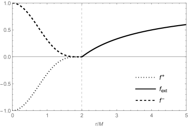
Figure 1: Metric function $f=f(r)$ for BH (dotted line) and mimicker (dashed line) for ${\cal M}/M\approx\,1.0$, $n=2$ and $k=4$. Dashed vertical line represents $r=r_{\rm s}$ (in units of $\cal M$).

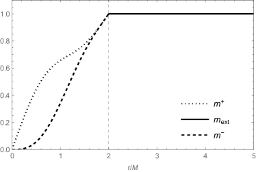
Figure 2: Mass function $m=m(r)$ for BH (dotted line) and mimicker (dashed line) for ${\cal M}/M\approx\,1.0$, $n=2$ and $k=4$. Dashed vertical line represents $r=r_{\rm s}$ (in units of $\cal M$).

The next step is to extend our solutions (2) with $\Phi=0$ and $m=m^{\pm}(r)$ to the region $r>r_{\rm s}$. First of all, it is easy to prove that these solutions cannot be smoothly joined with the Schwarzschild vacuum at $r=r_{\rm s}$ Ovalle (2023). In fact, the metric of this vacuum is also of the form in Eq. (2) with $\Phi=0$ and constant mass function $m=\mathcal{M}$. Hence, $m^{\prime}(r_{\rm s}^{+})=0$ cannot equal the derivative of $m^{\pm}(r_{\rm s}^{-})$.

An exterior metric (for $r>r_{\rm s}$) of the form in Eq. (2) with $\Phi=0$, which smoothly matches the interiors with the mass functions $m=m^{\pm}(r)$ at $r=r_{\rm s}$, and approaches the Schwarzschild metric for $r\gtrsim r_{\rm s}$, is given by 

$$f_{\rm ext}=1-\frac{{2\,\cal M}}{r}-\left(1-\frac{{2\,\cal M}}{r_{\rm s}}\right)\exp\left\{-2\,\frac{r-r_{\rm s}}{2\,\mathcal{M}-\ell}\right\}\ ,$$ (23)

where $\mathcal{M}$ is the ADM mass (measured by an asymptotic observer) and $\ell$ a length scale which must satisfy ${\cal M}\leq\ell<2\,{\cal M}$ in order to ensure asymptotic flatness and also have

$$r_{\rm s}=2\,M={\cal M}+\sqrt{\ell\,{\cal M}-{\cal M}^{2}}\ .$$ (24)

It is important to remark the difference between ${\cal M}$ and $M$ in Eq. (12). The former is the total mass of the configuration, while the latter is the fraction of mass confined within the region $r\leq r_{\rm s}$. Indeed, from the expression in Eq. (24) we see that $M<{\cal M}\leq 2\,M$, with

$$\ell\to 2\,{\cal M}\quad\Rightarrow\quad{\cal M}\to M\ .$$ (25)

Hence we conclude that $\ell$ controls the amount of mass ${\cal M}$ contained within the trapping surface $r=r_{\rm s}$. The case $\ell\to 2\,{\cal M}$ in Eq. (25) would correspond to the Schwarzschild BH with the total mass ${\cal M}=M$ confined within the region $r\leq r_{\rm s}$. However, we have seen that this limiting case is excluded and we can conclude that both integrable BHs and mimickers are dressed with a shell of matter of (arbitrarily small) thickness $\Delta\simeq 2\,{\cal M}-\ell>0$ and (arbitrarily small) mass ${\cal M}-M\simeq\Delta/4$ (for example, $\Delta/r_{\rm s}\simeq 0.05$ in Figs. 1 and 2).

III.3 Complete geometries

By matching the interior for $m=m^{+}$ with the exterior (23) one obtains a complete BH geometry. Likewise, a mimicker is obtained by joining the exterior (23) to the interior with $m=m^{-}$ (see Figs. 1 and 2 for an example). In particular, we note that the continuity of the mass function across $r_{\rm s}=2\,M$ means that $f_{\rm int}^{\pm}(r_{\rm s}^{-})=0=f_{\rm ext}(r_{\rm s}^{+})$ and continuity of $m^{\prime}$ implies that $f_{\rm ext}^{\prime}(r_{\rm s}^{+})=0=(f_{\rm int}^{\pm})^{\prime}(r_{\rm s}^{-})$.

We would like to highlight a few more features of these two solutions:

• Both solutions contain only two charges, i.e. the ADM mass ${\cal M}$ and the length scale $\ell=2\,\mathcal{M}-\Delta$.

• A BH and a mimicker can have the same exterior geometry with ADM mass $\cal M$ provided the interior mass $M=m^{\pm}(r_{\rm s})$ (equivalently $\ell$) is also the same.

• The sphere $r=r_{\rm s}$ is an event horizon for the BH and an infinite redshift hypersurface for the mimicker.

• The interior $r\leq r_{\rm s}$ is quite different in the two cases: the BH has one horizon (there is no Cauchy inner horizon), and contains an integrable singularity at $r=0$ [see Eq. (17)]; the mimicker is completely regular inside.

We also remark that there is a discontinuity in the tangential pressure $p_{\theta}\sim m^{\prime\prime}$ at $r=r_{\rm s}$ Ovalle (2023); Ovalle et al. (2021).

IV From de Sitter to anti-de Sitter

We have seen that the the mass functions in Eq. (11) can correspond to static BHs and mimickers. We can now consider the possibility of dynamical processes that result in the transition between two such configurations. In general, the ADM mass $\cal M$ and radius $r_{\rm s}=2\,M$ (equivalently, the length scale $\ell$) could change in time. However, it is easier to consider cases in which both parameters remain constant.

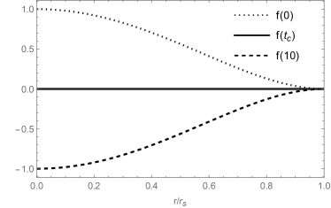
Figure 3: Metric function $f$ for mimicker-to-BH with $k=2$ at different times ($t$ in units of $\omega^{-1}$) and $t_{\rm c}$ in Eq. (29).

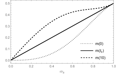
Figure 4: Mass function $m$ for mimicker-to-BH with $k=2$ at different times ($t$ in units of $\omega^{-1}$) and $t_{\rm c}$ in Eq. (29).

In particular, since the BH metric with mass function $m=m^{+}$ involves a larger fraction of the total mass near the centre than the mimicker with $m=m^{-}$ (see Fig. 2), it makes sense to assume that the mimicker represents the initial configuration and the BH is the final configuration for this process (the opposite may be more interesting for cosmology, see Appendix B). This means that the mass function for $0\leq r\leq r_{\rm s}$ must be time dependent, $m=m(r,t)$ (see also Appendix C), and start from the mimicker with $f=f^{-}$, say at $t=0$,

$$m(r,t=0)=m^{-}(r;r_{\rm s})\ .$$ (26)

to evolve into the BH with $f=f^{+}$, at least in an infinite amount of time,

$$m(r,t\to\infty)=m^{+}(r;r_{\rm s})\ ,$$ (27)

with $r_{\rm s}=2\,M$ at all times. The exterior geometry is instead static and described by $f_{\rm ext}$ in Eq. (23) with constant $\cal M$ and $\ell$ related with $r_{\rm s}$ according to Eq. (24).

An example of a time-dependent mass function for the interior with the above features is given by

$$m(r,t)=\frac{r}{2}\left\{1+\left(1-2\,e^{-\omega\,t}\right)\left[1-\left(\frac{r}{r_{\rm s}}\right)^{2}\right]^{k}\right\}\ ,$$ (28)

where $\omega^{-1}$ is a time scale associated with the transition. In this respect, it is interesting to note that the complete spacetime metric changes signature across $r=r_{\rm s}$ (and the surface $r=r_{\rm s}$ becomes a horizon) at a time

$$t_{\rm c}=\ln(2)\,\omega^{-1}\ ,$$ (29)

when $f(r)=0$ and $m=r/2$ for $0\leq r\leq r_{\rm s}$ (see Figs. 3 and 4 for an example).

Since the exterior geometry does not change, one can look at this process as being consistent with the fact that $r=r_{\rm s}$ is a sphere of infinite redshift for all $t>0$. Mechanisms to allow for energy loss must therefore involve quantum effects, like the Hawking evaporation Hawking (1975), which we have neglected here.

V Conclusion and final remarks

Studying the possible evolution from (horizonless) ultracompact objects to BHs using purely analytical and exact models, is a great challenge. In this sense, the model represented by the mass function in Eq. (28) could be pioneering in this scenario. Its generalisation to more complex and realistic situations could help to shed light on new aspects of the gravitational collapse, in particular, on the existence of ultracompact stellar configurations as the final stage.

Although Eq. (28) represents an advancement, it is fair to mention that our model is not free from limitations. One of them is the fact that external observers could never detect this specific transition from a mimicker to the BH in the classical theory. This is a direct consequence of the two (Cauchy horizon free) configurations in Eq. (11), which represent the initial and final states of our model, respectively. We can see that the BH horizon always coincides with the infinite redshift surface of the mimicker and, correspondingly, no energy is emitted (classically) during the process. In this form, our model is still a valid starting point to investigate near-horizon quantum physics.

We would like to conclude by emphasizing that we do not mean to provide a phenomenologically complete model. On the contrary, our objective is, more humbly but no less importantly, to lay the foundation for analytically exploring the collapse of ultra-compact configurations into BHs. In this perspective, there are many aspects that deserve further studying, such as its stability and extension to include energy emission and rotating systems. One should also consider alternative transitions from our mimickers, which are regular objects, to non-singular (rather than integrable) BHs, which will generically contain two horizons, namely the event horizon and the Cauchy horizon. All such aspects go beyond the scope of this article.

Acknowledgments

J.O. is partially supported by ANID FONDECYT Grant No. 1210041. R.C. and A.K. are partially supported by the INFN grant FLAG. The work of R.C. has also been carried out in the framework of activities of the National Group of Mathematical Physics (GNFM, INdAM).

Appendix A Painlevé-Gullstrand coordinates

For the metric (2) with $\Phi=0$, one can introduce a Painlevé-Gullstrand time $T$ such that spatial hypersurfaces of constant $T$ are flat,

$$ds^{2}=-f\,dT^{2}+2\,\sqrt{1-f}\,dT\,dr+dr^{2}+r^{2}\,d\Omega^{2}\ .$$ (30)

We can next introduce tetrads which, for the angular part, read

$$e_{(2)}^{\mu} = \left(0,0,\frac{1}{r},0\right)$$

$$e_{(3)}^{\mu} = \left(0,0,0,\frac{1}{r\,\sin\theta}\right)\ .$$ (31)

Where $0<f\leq 1$, like inside the mimicker with $f=f^{-}$ and in the exterior with $f=f_{\rm ext}$, one can define two tetrads

$$e_{(0)}^{\mu} = \left(\frac{1}{\sqrt{f}},0,0,0\right)$$ (32)

$$e_{(1)}^{\mu} = \left(-{\sqrt{\frac{1}{f}-1}},\sqrt{f},0,0\right)\ .$$ (33)

Where $f<0$, like inside the BH with $f=f^{+}$, one can instead use

$$e_{(0)}^{\mu} = \left(-\sqrt{1-\frac{1}{f}},\sqrt{-f},0,0\right)$$ (34)

$$e_{(1)}^{\mu} = \left(\frac{1}{\sqrt{-f}},0,0,0\right)\ .$$ (35)

The effective energy-momentum tensor sourcing the metric can then be obtained by projecting the Einstein tensor on the tetrad. From

$$G^{T}_{\ T} = G^{r}_{\ r}=\frac{f+r\,f^{\prime}-1}{r^{2}}$$

$$G^{\theta}_{\ \theta} = G^{\phi}_{\ \phi}=\frac{2\,f^{\prime}+r\,f^{\prime\prime}}{2\,r}\ ,$$ (36)

one finds

$$\kappa\,\epsilon={G_{\mu\nu}\,e^{\mu}_{(0)}\,e^{\nu}_{(0)}}=\frac{2\,m^{\prime}}{r^{2}}\ .$$ (37)

Since the spatial metric is flat, it is now easy to see that the total energy within a sphere of radius $r$ at constant $T$ is indeed given by Eq. (22), regardless of the sign of $f$. Moreover the spatial volume of these hypersurfaces inside $r_{\rm s}$ is also constant and equals $(4/3)\,\pi\,r_{\rm s}^{3}$. Furthermore, the radial pressure

$$\kappa\,p_{r}={G_{\mu\nu}\,e^{\mu}_{(1)}\,e^{\nu}_{(1)}}=-\kappa\,\epsilon\ ,$$ (38)

and the tangential pressure

$$\kappa\,p_{\theta}=G_{\mu\nu}\,e_{(2)}^{\mu}\,e_{(2)}^{\nu}=G_{\mu\nu}\,e_{(3)}^{\mu}\,e_{(3)}^{\nu}=\kappa\,p_{\phi}=-\frac{m^{\prime\prime}}{r}\ .$$ (39)

All expressions are clearly in agreement with Eq. (5).

Appendix B Inside the black hole

Let us consider the geometry inside the horizon $r=r_{\rm s}$ for $n=2$ and $k=1$ [see Eq. (17)] as a whole universe, in the spirit of Ref. Doran et al. (2008). In this case the metric reads

$$ds^{2}=\frac{dt^{2}}{1-{t^{2}}/{t_{0}^{2}}}-\left(1-\frac{t^{2}}{t_{0}^{2}}\right)dr^{2}-t^{2}\,d\Omega^{2}\ .$$ (40)

The components of the Ricci tensor are

$$R_{\ t}^{t} = R_{\ r}^{r}=\frac{3}{t_{0}^{2}}$$

$$R_{\ \theta}^{\theta} = R_{\ \phi}^{\phi}=-\frac{2}{t^{2}}+\frac{3}{t_{0}^{2}}\ ,$$ (41)

and the Ricci scalar is

$$R=\frac{12}{t_{0}^{2}}-\frac{4}{t^{2}}\ .$$ (42)

The components of the Einstein tensor therefore read

$$G_{\ t}^{t} = G_{\ r}^{r}=-\frac{3}{t_{0}^{2}}+\frac{2}{t^{2}}$$

$$G_{\ \theta}^{\theta} = G_{\ \phi}^{\phi}=-\frac{3}{t_{0}^{2}}\ .$$ (43)

Comparing Eqs. (43) with the expression (4) for the energy-momentum tensor, we see that this universe is filled with a negative cosmological constant and an anisotropic fluid, in agreement with the analysis in Appendix A.

We can rewrite the metric (40) in terms of the cosmic time $\tau$ with

$$t=t_{0}\,\sin\left(\frac{\tau}{t_{0}}\right)\ ,$$ (44)

which yields

$$ds^{2}=d\tau^{2}-\cos^{2}\left(\frac{\tau}{t_{0}}\right)dr^{2}-t_{0}^{2}\,\sin^{2}\left(\frac{\tau}{t_{0}}\right)d\Omega^{2}\ .$$ (45)

This metric describes a Kantowski-Sachs universe with a simple form for the two scale factors Kantowski and Sachs (1966); Brehme (1977).

Appendix C Time-dependent energy-momentum tensor

The components of the energy-momentum tensor for a metric of the form (2) with $\Phi=0$ and $m=m(r,t)$ can be easily obtained from the Einstein equations (1) and read

$$T^{0}_{\ 0} = \frac{2\,{m}^{\prime}}{\kappa\,r^{2}}\ ,\quad T^{1}_{\ 1}=-\frac{2\,{m}^{\prime}}{\kappa\,r^{2}}=-T^{0}_{\ 0}\ ,$$

$$T^{2}_{\ 2} = -\frac{{m}^{\prime\prime}}{\kappa\,r}-\frac{4\,r\,{\dot{m}}^{2}}{\kappa\,(r-2\,m)^{3}}-\frac{r\,{\ddot{m}}^{2}}{\kappa\,(r-2\,m)^{2}}\ ,$$ (46)

where dots denote derivatives with respect to $t$. These expressions reduce to those in Appendix A for the static case $\dot{m}=0$. Moreover, one also finds a flux of energy

$$T^{0}_{\ 1}=-\frac{2\,{\dot{m}}}{\kappa\,(r-2\,m)^{2}}\ ,$$ (47)

which does not appear in the static case.

The (apparently) singular behaviour of terms containing $\dot{m}$ and $\ddot{m}$ for $r\to 2\,m$ is just due to the choice of Schwarzschild-like coordinates in Eq. (2). One can remove this apparent singularity by employing Eddington-Finkelstein coordinates, in which the metric reads

$$ds^{2}=-f\,dv^{2}+2\,dv\,dr+r^{2}\,d\Omega^{2}\ ,$$ (48)

and the components of the energy-momentum tensor equal those in Eq. (5) with $T^{0}_{\ 1}=0$.

References

- Mazur and Mottola (2004) P. O. Mazur and E. Mottola, Proc. Nat. Acad. Sci. 101, 9545 (2004), arXiv:gr-qc/0407075 .
- Mazur and Mottola (2023) P. O. Mazur and E. Mottola, Universe 9, 88 (2023), arXiv:gr-qc/0109035 .
- Visser and Wiltshire (2004) M. Visser and D. L. Wiltshire, Class. Quant. Grav. 21, 1135 (2004), arXiv:gr-qc/0310107 [gr-qc] .
- Lobo (2006) F. S. N. Lobo, Class. Quant. Grav. 23, 1525 (2006), arXiv:gr-qc/0508115 .
- Lukash and Strokov (2013) V. N. Lukash and V. N. Strokov, Int. J. Mod. Phys. A 28, 1350007 (2013), arXiv:1301.5544 [gr-qc] .
- Casadio (2022) R. Casadio, Int. J. Mod. Phys. D 31, 2250128 (2022), arXiv:2103.00183 [gr-qc] .
- Casadio et al. (2022) R. Casadio, A. Giusti, and J. Ovalle, Phys. Rev. D 105, 124026 (2022), arXiv:2203.03252 [gr-qc] .
- Casadio et al. (2023) R. Casadio, A. Giusti, and J. Ovalle, JHEP 05, 118 (2023), arXiv:2303.02713 [gr-qc] .
- Carballo-Rubio et al. (2023) R. Carballo-Rubio, F. Di Filippo, S. Liberati, and M. Visser, (2023), arXiv:2302.00028 [gr-qc] .
- Visser (1995) M. Visser, Lorentzian wormholes: From Einstein to Hawking (1995).
- Misner and Sharp (1964) C. W. Misner and D. H. Sharp, Phys. Rev. 136, B571 (1964).
- Hernandez and Misner (1966) W. C. Hernandez and C. W. Misner, Astrophys. J. 143, 452 (1966).
- Kerr and Schild (1965) R. P. Kerr and A. Schild, Proc. Symp. Appl. Math 17, 199 (1965).
- Ovalle (2017) J. Ovalle, Phys. Rev. D95, 104019 (2017), arXiv:1704.05899 [gr-qc] .
- Ovalle (2019) J. Ovalle, Phys. Lett. B788, 213 (2019), arXiv:1812.03000 [gr-qc] .
- Ovalle (2023) J. Ovalle, Phys. Rev. D 107, 104005 (2023), arXiv:2305.00030 [gr-qc] .
- Arnowitt et al. (1959) R. L. Arnowitt, S. Deser, and C. W. Misner, Phys. Rev. 116, 1322 (1959).
- Martin-Moruno and Visser (2017) P. Martin-Moruno and M. Visser, Fundam. Theor. Phys. 189, 193 (2017), arXiv:1702.05915 [gr-qc] .
- Ovalle et al. (2021) J. Ovalle, R. Casadio, E. Contreras, and A. Sotomayor, Phys. Dark Univ. 31, 100744 (2021), arXiv:2006.06735 [gr-qc] .
- Hawking (1975) S. W. Hawking, Commun. Math. Phys. 43, 199 (1975), [Erratum: Commun.Math.Phys. 46, 206 (1976)].
- Doran et al. (2008) R. Doran, F. S. N. Lobo, and P. Crawford, Found. Phys. 38, 160 (2008), arXiv:gr-qc/0609042 .
- Kantowski and Sachs (1966) R. Kantowski and R. K. Sachs, J. Math. Phys. 7, 443 (1966).
- Brehme (1977) R. W. Brehme, Am. J. Phys. 45, 423 (1977).