scDiffusion: conditional generation of high-quality single-cell data using diffusion model

Abstract

Single-cell RNA sequencing (scRNA-seq) data are important for studying the biology of development or diseases at single-cell level. To better understand the properties of the data, to build controlled benchmark data for testing downstream methods, and to augment data when collecting sufficient real data is challenging, generative models have been proposed to computationally generate synthetic scRNA-seq data. However, the data generated with current models are not very realistic yet, especially when we need to generate data with controlled conditions. In the meantime, the Diffusion models have shown their power in generating data in computer vision at high fidelity, providing a new opportunity for scRNA-seq generation.

In this study, we developed scDiffusion, a diffusion-based model to generate high-quality scRNA-seq data with controlled conditions. We designed multiple classifiers to guide the diffusion process simultaneously, enabling scDiffusion to generate data under multiple condition combinations. We also proposed a new control strategy called Gradient Interpolation. This strategy allows the model to generate continuous trajectories of cell development from a given cell state.

Experiments showed that scDiffusion can generate single-cell gene expression data closely resembling real scRNA-seq data, surpassing state-of-the-art models in multiple metrics. Also, scDiffusion can conditionally produce data on specific cell types including rare cell types. Furthermore, we could use the multiple-condition generation of scDiffusion to generate cell type that was out of the training data. Leveraging the Gradient Interpolation strategy, we generated a continuous developmental trajectory of mouse embryonic cells. These experiments demonstrate that scDiffusion is a powerful tool for augmenting the real scRNA-seq data and can provide insights into cell fate research.

1 Introduction

Single-cell RNA sequencing (scRNA-seq) data offer comprehensive depictions of the gene expression profile of every single cell, which can help gain a more systematic and precise understanding of the development and function of living organisms [1, 2]. Although current sequencing technologies have come a long way, the cost and difficulty of sequencing remain high. Besides, the biological samples are sometimes hard to be obtained due to ethical reasons [3, 4, 5], and certain cell types within a sample may be too rare to be analyzed. It is still challenging to obtain enough high-quality scRNA-seq data of interest, which may impede biological discovery as most tools for scRNA-seq analysis require a certain amount of high-quality data.

Some researchers have tried to generate in silico gene expression data in response to the less-than-desirable availability of scRNA-seq data. Unlike single-cell sequencing technologies that need real biological samples, the in silico data generation methods aim to generate pseudo data according to the expression pattern of known data. There are two main types of in silico data generation methods: statistical modelling and deep learning. Statistical modeling methods are guided by well-studied statistical distributions of gene expression profiles such as Zero-inflated Negative Binomial (ZINB) [6], and new data are generated by manually setting certain parameters of the distributions [7, 8, 9, 10]. However, due to the over simplification of statistical models, these methods can hardly mimic the real gene expression data exactly, but are mainly used as toy data for guiding the development of scRNA-seq analysis algorithms.

The recent prosperity of deep generative models brings new chances for the in silico transcriptomic data generation [11]. Deep generative models can learn the biological patterns of single-cell gene expression without any explicit modeling, which makes it possible to generate realistic scRNA-seq data. The variational autoencoder (VAE) is one of the most prominent deep generative models in the field [12]. A classic example of a VAE-based data generation model is the single-cell variational inference (scVI), which guide a VAE to infer underlying data distributions by generating data similar to original data [13]. However, these VAE-based models are designed to approximate the data distributions for downstream analysis tasks such as batch correction and clustering, rather than generating pseudo gene expression profiles of cells. Recently, the generative adversary network (GAN) [14] was utilized to develop tools specializing in generating new cells. For example, scGAN uses a deep learning model to learn the non-linear gene-gene dependencies from different cell samples, and then generates realistic scRNA-seq data according to the information it learns, achieving very impressive results in many evaluation metrics [15]. There are several variations of the scGAN model, such as LSH-GAN[16] and scIGAN[17], both of which utilize the generative capabilities of GAN to accomplish downstream tasks in single-cell analysis. Though, the scGAN model is specifically designed to generate data from a known distribution, and cannot be used to supplement unmeasured data. Besides, GAN requires careful design and tuning of model architectures and optimization methods to achieve stable training results [18], which may cause trouble when generalizing the GAN-based methods to other datasets.

The diffusion model [19] is the most trending generative model at the moment and has demonstrated excellent performance in a number of areas such as generating images and audios [20, 21]. It has many desirable properties like distribution coverage, a stationary training objective, and easy scalability, and has outperformed previous works in terms of generating significantly higher-quality data [22, 23, 24]. While the diffusion model has yielded great results in many fields, it has few applications in the single-cell area. The primary challenge lies in the fact that the distribution of scRNA-seq data significantly deviates from the Gaussian distribution, unlike image data which inherently exhibit a Gaussian-like distribution. This makes it difficult for diffusion models to generate new gene expression data, as the entire diffusion process is based on Gaussian noise.

In this paper, we propose scDiffusion, a novel in silico scRNA-seq data generation model based on the structure of the denoising diffusion probability model, to generate single-cell gene expression data with given conditions. scDiffusion mainly consists of three parts, an autoencoder, a diffusion backbone, and a condition controller. The autoencoder helps rectify the raw distribution and reduce the dimensionality of scRNA-seq data, which can make the data amenable to diffusion modeling. The backbone model was redesigned based on a multilayer perceptron (MLP) to make the model adaptable to the unordered nature of gene expression data. The conditional controller is a cell type classifier, enabling scDiffusion to generate data specific to a particular cell or organ type according to diverse requirements. scDiffusion was shown to be able to generate realistic scRNA-seq data which surpassed the data generated by scGAN in various evaluation metrics. We further demonstrated the ability of scDiffusion on conditional generation, multi-conditional generation capacity, and out-of-distribution data generation. We also proposed a novel condition control strategy, Gradient Interpolation, to interpolate continuous cell trajectories from discrete cell states. With the powerful generation ability, scDiffusion has the potential to augment existing scRNA-seq data and could potentially contribute to the investigation of undersampled or even unseen cell states.

2 Methods

The scDiffusion model consists of three parts, an autoencoder, a diffusion backbone network, and a conditional classifier, as depicted in Fig. 1. The autoencoder is designed to transform the raw gene expression profiles into latent space embeddings to effectively reduce dimensions and ensure a more suitable distribution for the subsequent diffusion process. The diffusion backbone network is designed to learn the reversed diffusion process. Meanwhile, the conditional classifier provides guidance for the reverse diffusion, allowing the generation of cells under specific conditions such as specific cell types or organs.

At the training stage, the autoencoder is first trained to embed the gene expression profile of every single cell by using all real gene expression data. After, the diffusion process is applied to each embedding derived by the autoencoder and produces a series of noisy embeddings. These noisy embeddings serve as the training data for the backbone network. Meanwhile, the conditional classifier processes the embeddings to predict associated labels, such as cell types. At the inference stage, the diffusion backbone denoises the input noise embeddings and generates new embeddings. The generation can be guided by the classifier or the Gradient Interpolation strategy. The generated embeddings are finally fed into the decoder to obtain full gene expression. Detailed descriptions of scDiffusion are provided below.

Figure 1: The overall structure of scDiffusion.

2.1 Training the gene expression autoencoder

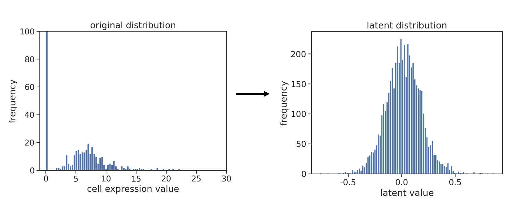
Figure S1: Distribution of original gene expression and latent embeddings derived by the autoencoder.

The dimensions of gene expression data are extremely high, and the data distribution differs from the Gaussian distribution used in the diffusion process. To solve this problem, we used an autoencoder consisting of two MLPs to encode the gene expression data of every single cell $S_{ori}$ into a latent space embedding $x_{0}$. The input of the encoder is a gene expression profile that is normalized by 1e4 total counts, and the output is a 1,000-dimension latent space embedding. The decoder subsequently accepts the latent space embedding and generates the corresponding expression profile $S_{new}$ as the output. As shown in Fig. S1, the distribution of gene expression is transformed into a Gaussian-like distribution by the autoencoder, which is in line with the Gaussian distribution used in the diffusion process and makes it much easier for the backbone model to learn the reverse process.

2.2 Training the diffusion backbone network

After getting embeddings from the encoder, the diffusion process is applied to each embedding. The diffusion backbone network is trained to learn the reversed process. Classical diffusion backbone models such as convolutional neural networks are not applicable to gene expression, as a gene expression profile of scRNA-seq data is a long, sparse, and unordered vector. Thus, we developed a new architecture as the backbone, with fully connected layers and a residual structure (Fig. 1). The residual structure can help to maintain the characteristics of features at different levels and reduce the loss of information.

In the diffusion process, the original cell embedding $x_{0}$ becomes a noised embedding $x_{T}$ by iteratively adding noise through $T$ steps. For the $i$-th step, the embedding $x_{i}$ is sampled from the following distribution:

$$q\left(x_{i}\middle|x_{i-1}\right)=\mathcal{N}\left(x_{i}\middle|\sqrt{1-\beta_{i}}x_{i-1},\beta_{i}I\right),~{}~{}\mathrm{where}\quad\beta_{i}\in(0,1)$$ (1)

where $I$ stands for standard Gaussian noise. $\beta_{i}$ is a coefficient that varies with time step, and $\beta_{min}$ and $\beta_{max}$ are two parameters that control the scale of $\beta_{i}$ in the diffusion process:

$$\beta_{i}=\frac{\beta_{min}}{T}+\frac{i-1}{T-1}\left({\frac{\beta_{max}}{T}-\frac{\beta_{min}}{T}}\right)$$ (2)

The training goal is to learn the reverse diffusion process $p(x_{i-1}|x_{i})$. In each iteration, $x_{i-1}$ at step $i-1$ is predicted, given an embedding $x_{i}$ at step $i$. Such process also follows the Gaussian distribution. According to previous works [19, 22], the mean and variance are parameterized as:

$$p_{\theta}(x_{i-1}|x_{i})=\mathcal{N}(x_{i-1}|\mu_{\theta}(x_{i},i),\mathrm{exp}({w\beta}_{i}){I})$$ (3)

where $w$ in the variance is an adjustable weight that controls the randomness of the reverse process. The mean $\mu_{\theta}(x_{i},i)$ can be written as:

$$\mu_{\theta}(x_{i},i)=\frac{1}{\sqrt{\alpha_{t}}}\left(\mathbf{x}_{t}-\frac{\beta_{t}}{\sqrt{1-\bar{\alpha}_{t}}}\boldsymbol{\epsilon}_{\theta}\left(\mathbf{x}_{t},t\right)\right)$$ (4)

where $\alpha_{t}=1-\beta_{t}$ and $\bar{\alpha}_{t}=\prod_{s=1}^{t}\alpha_{s}$. ${\epsilon}_{\theta}\left(x_{i},i\right)$ is the added noise predicted by the backbone network. In other words, the backbone network takes the cell’s latent space embedding $x_{i}$ and the timestamp $i$ as inputs to predict the noise.

In the inference process, the diffusion model takes the Gaussian noise as the initial input and denoises it iteratively through T steps. Eventually, we can get the new cellular latent space embedding $x_{0}$ and put it into the decoder to get the final gene expression data.

2.3 Conditional generation and the Gradient Interpolation strategy

We use the classifier guidance method to perform conditional generation. This method does not interfere with the training of the diffusion backbone model. Instead, the classifier is first trained separately by using condition labels like cell types and then provides a gradient to guide cell generation. Here, we designed the cell classifier as a four-layer MLP. After generating a series of embeddings from cells with labels, the classifier takes both timestamp $i$ and cell embedding $x_{i}$ as inputs and predicts the cell labels $y$ paired with $x_{0}$. The cross entropy loss is used for training. It is worth noting that only the embeddings between step $0$ and step $T/2$ of the diffusion process are used for training the classifier, considering that the signal in the rest part is too noisy to be predicted.

As for inference, given each step $i$ between the last part of the reverse process (between timestamp 0 and $T/2$), the classifier receives the intermediate state $x_{i}$ and outputs the predicted probability for every cell type. By computing the cross entropy loss between the predicted and desired condition given by the user, the gradient derived from the classifier can guide the diffusion backbone model to generate a designated endpoint. The new embedding with the guidance is now sampled from:

$$p_{\theta}(x_{i-1}|x_{i},y)=\mathcal{N}(x_{i-1}|\mu_{\theta}(x_{i},I)+\beta_{i}\gamma\nabla_{x_{i}}{\log p_{\phi}}\left({y\mid x_{i}}\right),\mathrm{exp}({w\beta}_{i}){I})$$ (5)

where $p_{\phi}\left(y\mid x_{i}\right)$ stands for the classifier’s result, and $\gamma$ is a weight that controls the effectiveness of the classifier to the reverse process. $\phi$ indicates the trainable parameters in the classifier. This guidance will affect every step of the reverse process and finally help the model’s output reach a certain condition.

Since the classifier is trained aside from the diffusion model and is only used in the inference stage, we can train multiple classifiers {$\phi_{1},\phi_{2},...$} to control different conditions separately. The gradient that guides the diffusion process is the summation of all the classifiers’ gradients with different weights {$\gamma_{1},\gamma_{2},...$}.

We proposed a Gradient Interpolation strategy to generate continuous cell condition guidance. A classifier receives two different conditions such as the initial and end state of cell differentiation, and generates two gradients at the same time. These gradients are then integrated to guide the diffusion to an unseen intermediate state. Specifically speaking, the $\beta_{i}\gamma\nabla_{x_{i}}{\log p_{\phi}}\left({y\mid x_{i}}\right)$ in Eq. 5 is replaced by:

$$\beta_{i}\gamma\nabla_{x_{i}}{\log p_{\phi}}\left({y\mid x_{i}}\right)\rightarrow\beta_{i}(\gamma_{1}\nabla_{x_{i}}{\log p_{\phi}}\left({y_{1}\mid x_{i}}\right)+\gamma_{2}\nabla_{x_{i}}{\log p_{\phi}}\left({y_{2}\mid x_{i}}\right))$$ (6)

where $\gamma_{1}$ and $\gamma_{2}$ represent two adjustable coefficients that control the distance between the generated cells and the two target cell states. By tuning these coefficients, scDiffusion can decide which cell state the generated cell is closer to, thus generating cells with continuous states. With this strategy, the initial state of the diffusion generation process is changed from pure Gaussian noise to the latent space embedding of cells of the initial condition, following a noise addition process:

$$x_{init}=\sqrt{\alpha_{t}}x_{0}+\sqrt{1-\alpha_{t}}\epsilon$$ (7)

where $x_{init}$ is the initial state, and $t$ is a parameter that is smaller than the total diffusion step. $\alpha_{t}$ is the same thing as in Eq. 4. This modification preserves the general characteristics of the initial cells, allowing the model to generate a series of new cell states for each given initial state. These generated cells can constitute a continuous trajectory of cell states.

2.4 Evaluation metrics

To compare similarity between generated and real cells, we evaluated the generated data with various metrics. The statistical indicators consist of Spearman Correlation Coefficient (SCC), Pearson Correlation Coefficient (PCC), Maximum Mean Discrepancy (MMD) [25], local inverse Simpson’s index (LISI) [26]. and quantile-quantile plot (QQ-plot). We normalized the gene expression data of generated and real cells and calculated SCC and PCC between them. The LISI score was calculated on the data-integrated KNN graph by using the Python package scib [27]. We used the top 50 principle components (PCs) of real and generated cells to calculate MMD. The QQ-plot was drawn using both real and generated expression data of a specific gene.

The non-satistical metrics include Uniform Manifold Approximation and Projection (UMAP) visualization [28], marker gene expression, CellTypist classification [29], and random forest evaluation. The UMAP plot was used to visualize the generated and real expression data on a two-dimensional plane to provide a subjective judgment for the generated data. Similar to scGAN, we projected the generated cells on the first 50 PCs that were computed from the real cells, and then drew UMAP based on these features. The cell type in unconditionally generated data is classified by CellTypist, a classifier trained with real cell data by using the cell type as the label [29]. CellTypist is also used to judge whether the conditionally generated data can be classified into the right type. The random forest evaluation shares the same idea with scGAN, which uses a random forest model with 1000 trees and 5 maximum depths to distinguish cells from real and generated, and the more similar these two cells are, the closer the area under the receiver operating characteristic (ROC) curve (AUC) metric of random forests is close to 0.5.

3 Results

We conducted four experiments to demonstrate the capability of scDiffusion. First, we investigated the unconditional data generation ability of scDiffusion and compared it with scGAN. We then assessed scDiffusion on a conditional generation task to generate specific cell types. Furthermore, we applied scDiffusion in a multi-conditional generation case with both cell types and organs as conditions and used it to generate new cells under an unseen condition which is out of the distribution of the training data. Lastly, we employed the Gradient Interpolation strategy to generate intermediate states in cell reprogramming.

We employed three single cell transcriptomic datasets in these experiments. The PBMC68k dataset [30] is a classical scRNA-seq dataset that contains 11 different cell types of human peripheral blood mononuclear cells (PBMCs). As the CD4+ T helper 2 cells had an extremely low number and could not be classified by CellTypist, we removed them for downstream analysis. Tabular Muris [31] is a large-scale single cell transcriptomic database of mice across 12 organs. The Waddington-OT dataset [32] is a cell reprogramming dataset of mouse embryonic fibroblasts (MEFs), containing cells with different timestamps during an 18-day reprogramming process. For all three datasets, we filtered out cells with less than 10 expression counts and genes that expressed in less than 3 cells.

In all experiments, we set the diffusion step to 2000. The parameter $\gamma$ in Eq. 5 was set to 8 for the conditional generation of PBMC68k data and the intermediate state generation, and it was set to 2 for all other experiments. The parameter $w$ in Eq. 3 and Eq. 5 was set to 0.5. The parameter $t$ in Eq. 7 was set to 1800.

3.1 Realistic scRNA-seq data generation

We applied scDiffusion on the Tabular Muris dataset to generate new cells (Fig. 2a). For comparison, we also generated cells with scGAN using its default parameter setting. We evaluated the performance of scDiffusion and scGAN with various metrics, and the results indicated that scDiffusion can generate more realistic scRNA-seq data, achieving a SCC of 0.932, a MMD of 0.059, and a LISI score of 0.88, while scGAN’s results were 0.867, 0.065, and 0.66, respectively. The Random Forest AUC score for scDiffusion in the test set was 0.61, also outperforming scGAN’s 0.78 (Fig. 2b). We also trained scGAN and scDiffusion on the PBMC68k dataset, which showed a very similar result to the Tabular Muris dataset (Fig. 2c). The SCC, MMD and LISI between the scDiffusion-generated cells and real cells were 0.84, 0.013, and 0.91, respectively, while the results of scGAN were 0.89, 0.019, 0.88. The Random Forest result shown in Fig. 2d also demonstrated the outperformance of scDiffusion.

For the Tabular Muris dataset, we selected five transcription factors (Klf13, Ybx1, Hnrnpk, Cnbp, Hmgb2) that have the highest mean Gini importance when making cell type classification in the original paper [31]. We calculated the mean expression level of every marker in different cell types for real and scDiffusion-generated data, respectively, and then calculated PCCs between them. For the PBMC68k dataset, we selected several marker genes, including CD3D, CD8A, NKG7 [33], CD79A [34], CCR10 [35], and S100A8 [36] and did the same calculation. PCCs of all these genes are larger than 0.98. The distributions of expression of these genes in real and generated data also showed to be similar (Fig. 2e, 2f, S2, and S3). We also draw the QQ-plots of these genes in different cell types between real and generated data (Fig. S4). All these results show that scDiffusion can generate realistic data.

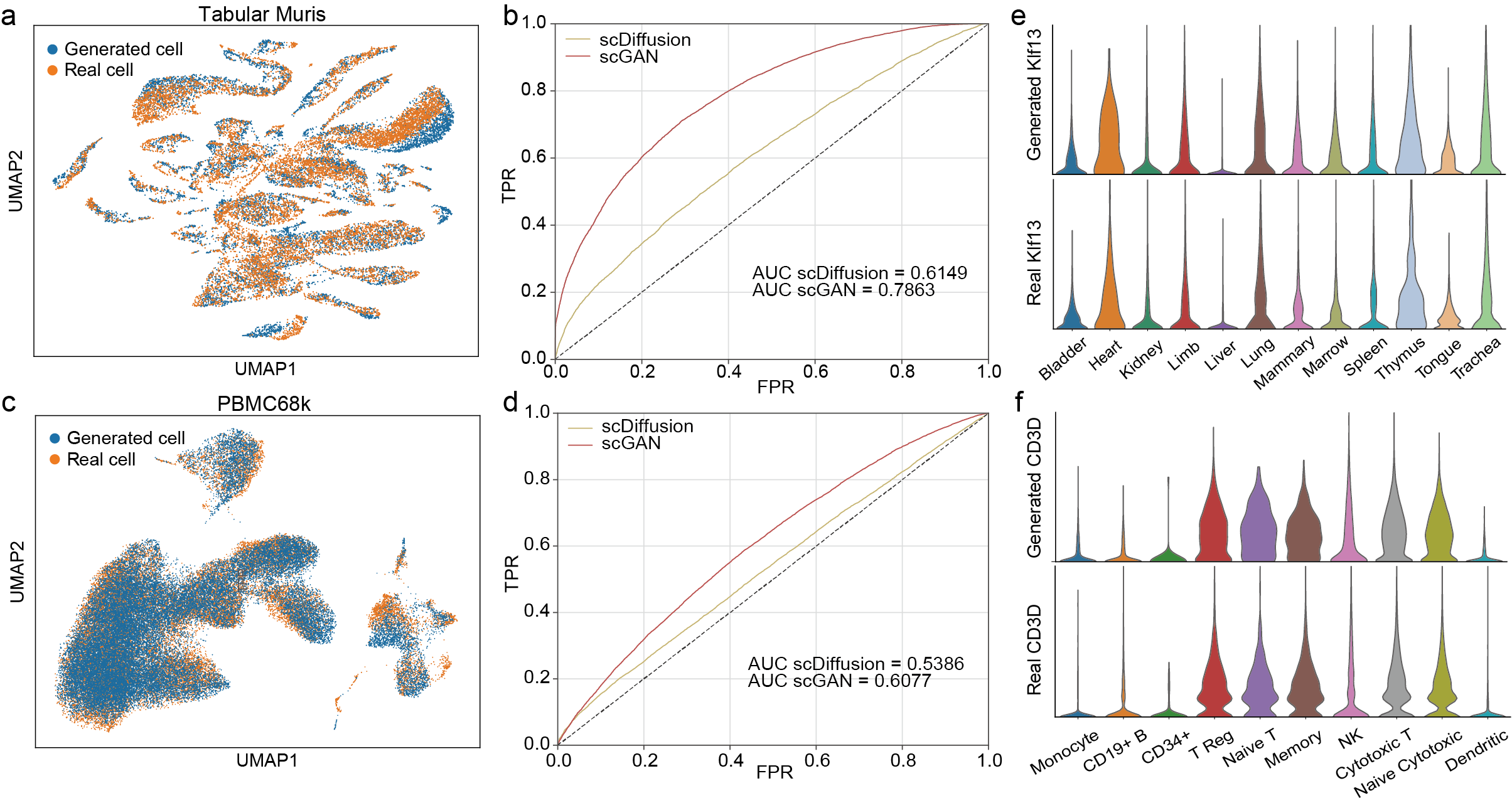
Figure 2: scDiffusion can generate realistic cell data. (a) UMAP of scDiffusion-generated Tabular Muris data and real Tabular Muris data. (b) Random Forest ROC curve of different methods in the Tabular Muris dataset. (c) UMAP of scDiffusion-generated PBMC68k data and real PBMC68k data. (d) Random Forest ROC curve of different methods in the PBMC68k dataset. (e) The expression of marker gene Klf13 in different cell types in the real and generated Tabular Muris data. (f) The expression of marker gene CD3D in different cell types in the real and generated PBMC68k data.

3.2 Conditionally generating specific cell types

We trained a cell type classifier according to the annotation provided by the Tabular Muris dataset to to guide the conditional generation of scDiffusion. For each cell type, we conditionally generated the same number of cells as the real data. As shown in Fig. 3a and S5, the conditionally generated cells visually overlapped with the real cells on the UMAP plot. We used Celltypist to classify these conditionally generated cells. As shown in Fig. 3b, the classification accuracies of the generated cells are close to those of the real cells in the test set. We also performed a similar procedure on the PBMC68k dataset, and the results are similar (Fig. 3c and 3d). It’s worth mentioning that rare cell types, such as the Thymus cell in the Tabular Muris dataset (2.5% in the whole dataset) and the CD34+ cell in the PBMC68k dataset (0.4% in the whole dataset), can also be well generated.

We then investigated how different parameter settings for $\gamma$ and $w$ in Eq. 5 affect the generation results, taking CD19+ B cells in the PBMC68k dataset as an example. We found that as the weight of classifier guidance $\gamma$ increases and the noise of the reverse process $exp(\sigma_{i}\mathbf{w})\mathbf{\varepsilon}$ decreases, the generated cells of the specific condition exhibit a denser distribution, and thus the boundaries between this cell type and other cell types become more distinct, which leads to higher accuracies of CellTypist to classify cell types (Fig. 3e). At the meantime, as real cells often exhibit a dispersed distribution, the densely generated cells may not fill all possible regions of the real distribution. These unfilled regions can be easily distinguished by a Random Forest classifier, leading to a worse Random Forest AUC performance (Fig. 3f).

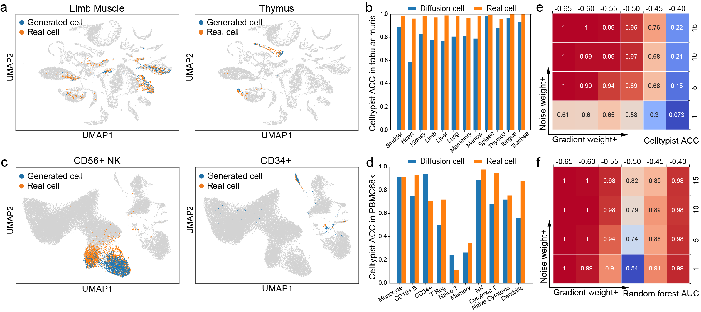
Figure 3: (a) UMAP of different cell types in the Tabular Muris dataset generated by conditional diffusion. The Thymus cell is a rare cell type. (b) The accuracy of CellTypist in different cell types in the Tabular Muris dataset. (c) UMAP of different cell types in the PPBMC68k dataset generated by conditional diffusion. The CD34+ cell is a rare cell type. (d) The accuracy of CellTypist in different cell types in the PBMC68k dataset. (e) The CellTypist accuracy of the CD19+ B cell with different parameter settings. (f) The Random Forest score of the CD19+ B cell with different parameter settings.

3.3 Generating out-of-distribution cell data with multiple conditions

We then tried to generate cells with multiple conditions baes on the Tabular Muris dataset. We trained two classifiers to separately control different conditions, one for organ type and the other for cell type. We selected three cell groups, mammary gland T cell, spleen T cell, and spleen B cell, from the dataset for training. We would like to generate cells with a new combination of conditions (mammary B cell) which was not seen in the training data, or in other words, out of the distribution of the training data.

As shown in Fig. 4, the generated cells with all combinations of conditions, including the out-of-distribution cells, visually overlapped with or near the real cells on the UMAP plot. The MMD score of the out-of-distribution cells was relatively higher than other generated cells (Fig. 4). We further trained a CellTypist model with all kinds of cells in mammary gland, and used it to classified the real and generated mammary gland B cells. The result showed that 85% of the generated cells and 91% of the real cells were categorized into the B cell. which showed that the scDiffusion can generate mammary B cells comparable to the real one. All the results suggested that scDiffusion can effectively generate realistic out-of-distribution mammary gland B cells by learning the expression patterns of both mammary gland cells and B cells.

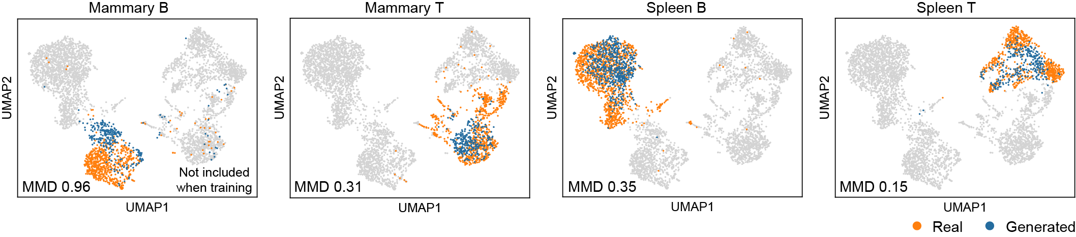
Figure 4: UMAP of real cells and cells generated with two conditions. The mammary gland B cells are unseen in the training data.

3.4 Generating intermediate cell states during cell reprogramming

We used the Gradient Interpolation strategy to generate the intermediate cell states during cell reprogramming in the Waddington-OT dataset. We trained scDiffusion on the Waddington-OT dataset, which contains MEFs with the induction of reprogramming to induced pluripotent stem cells (iPSCs). The data were across 18 days since induction with a half-day interval, and a part of the cells were induced to redifferentiate at day 8. We first chose all samples from day 0 to day 8 with the exception of day 0.5 and day 1 to train scDiffusion, and trained the classifier with the same dataset using the timestamp as the label. We then sent two conditions, day 0 and day 1.5, to the classifier and used Gradient Interpolation to generate a series of cell states between day 0 and day 1.5 in the development trajectory (Fig. 5a). The initial noise was set to be the noised latent space embeddings of day-0 cells.

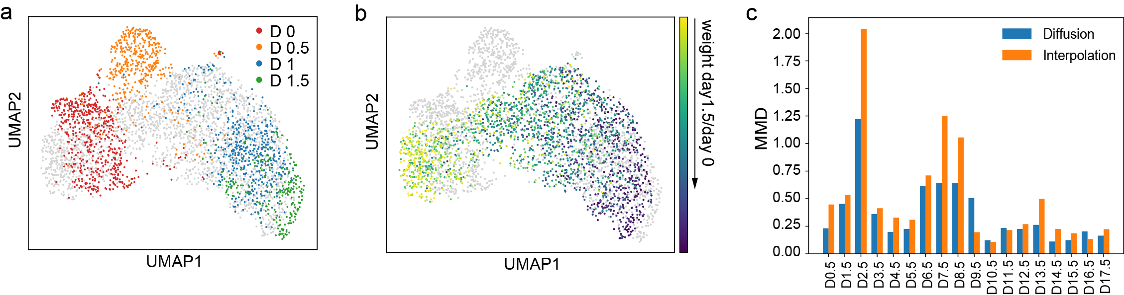
Figure 5: (a) UMAP of real cells. (b) UMAP of cells generated by Gradient Interpolation. (b) the MMD score of different methods at different timestamps.

We generated 20 states between day 0 and day 1.5 (Fig. 5b). We calculated the diffusion pseudotime [37] of different states (Fig. S6) and found that state 8 and state 18 are the closest to real cells of day 0.5 and day 1, respectively. These cells were previously stripped out from the training data. We compared these two states with the direct interpolation of day 0 and day 1.5 whose weight was the same as Gradient Interpolation. The MMD scores of state 8 and state 18 are 0.31 and 0.90, while the direct interpolation’s scores are 0.35 and 1.55. These results showed that scDiffusion can generate cells that are closer to the real intermediate state.

We also tried to train scDiffusion with all integer days and generate cells in the middle of two integer days. We compared the results with direct interpolation. As some of the cells were induced to redifferentiate at day 8, we interpolated cells within each treatment group separately. The interpolation weights of both methods were set to 1:1. As shown in Fig. 5c, scDiffusion exhibited better performance than direct interpolation in MMD metrics. The mean MMD of scDiffusion is 0.36, while the result of direct interpolation is 0.51, respectively. It is worth noting that scDiffusion was not trained with the information of different treatments, but its performance was still better than direct interpolation according to the treatment information, suggesting that the diffusion model can well capture the miscellaneous distribution of cells and well fit their intermediate states.

4 Discussion

In this paper, we present a deep generative neural network scDiffusion based on the denoising diffusion probability model. We use an autoencoder and a MLP-based backbone to enable diffusion models to be suitable for gene expression data, and generate realistic single cell data. By utilizing the classifier guidance method, scDiffusion can conditionally generate specific cell expression data based on user-defined conditions, including rare cell types. The flexibility of the classifier guidance also offers the potential to generate cells that are not seen in the training dataset. Furthermore, the Gradient Interpolation strategy enables the generation of a continuous cell trajectory between two known cell states to fill in intermediate states. These abilities can be used to augment available scRNA-seq data and hold the potential for analyzing cell states that are not sequenced.

With the powerful generative ability, scDiffusion has the prospect to carry on many other tasks. A very natural thing is multi-omics data generation. Theoretically, scDiffusion can generate any kind of single cell data. Besides, scDiffusion can also be used in the quality improvement of single cell data. For instance, by learning the overall expression paradigm in clean data, scDiffusion is able to perform denoising operations for contaminated data. In the future, we will try to replace the classifier with more powerful tools such as CLIP [38] in the stable diffusion [39]. In this way we may use more complex conditions to control the generating process and enable more complex tasks such as in silico cell perturbation, providing important help for drug selection and the control of cell state transition. The code of scDiffusion is available at https://github.com/EperLuo/scDiffusion.

5 Acknowledgements

The work is supported in part by National Key R&D Program of China (grant 2021YFF1200900), and National Natural Science Foundation of China (grants 62250005, 61721003, 62373210).

scDiffusion: conditional generation of high-quality single-cell data using diffusion model

Erpai Luo${}^{1,^{\#}}$, Minsheng Hao${}^{1,^{\#}}$, Lei Wei¹, Xuegong Zhang${}^{1,2,^{*}}$
 
¹MOE Key Lab of Bioinformatics and Bioinformatics Division of BNRIST,
Department of Automation, Tsinghua University, Beijing 100084, China
²School of Life Sciences and School of Medicine, Tsinghua University, Beijing 100084, China

Supplementary Materials

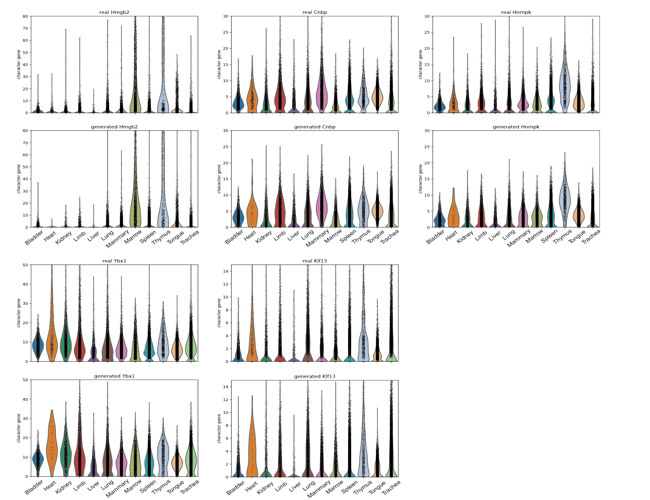
Figure S2: Expression of feature genes in the real and generated Tabular Muris data.

Figure S3: Expression of feature genes in the real and generated PBMC68k data.

Figure S4: QQ-plots of expression of feature genes in the real and generated data. (a) The Tabular Muris dataset. (b) The PBMC68k dataset.

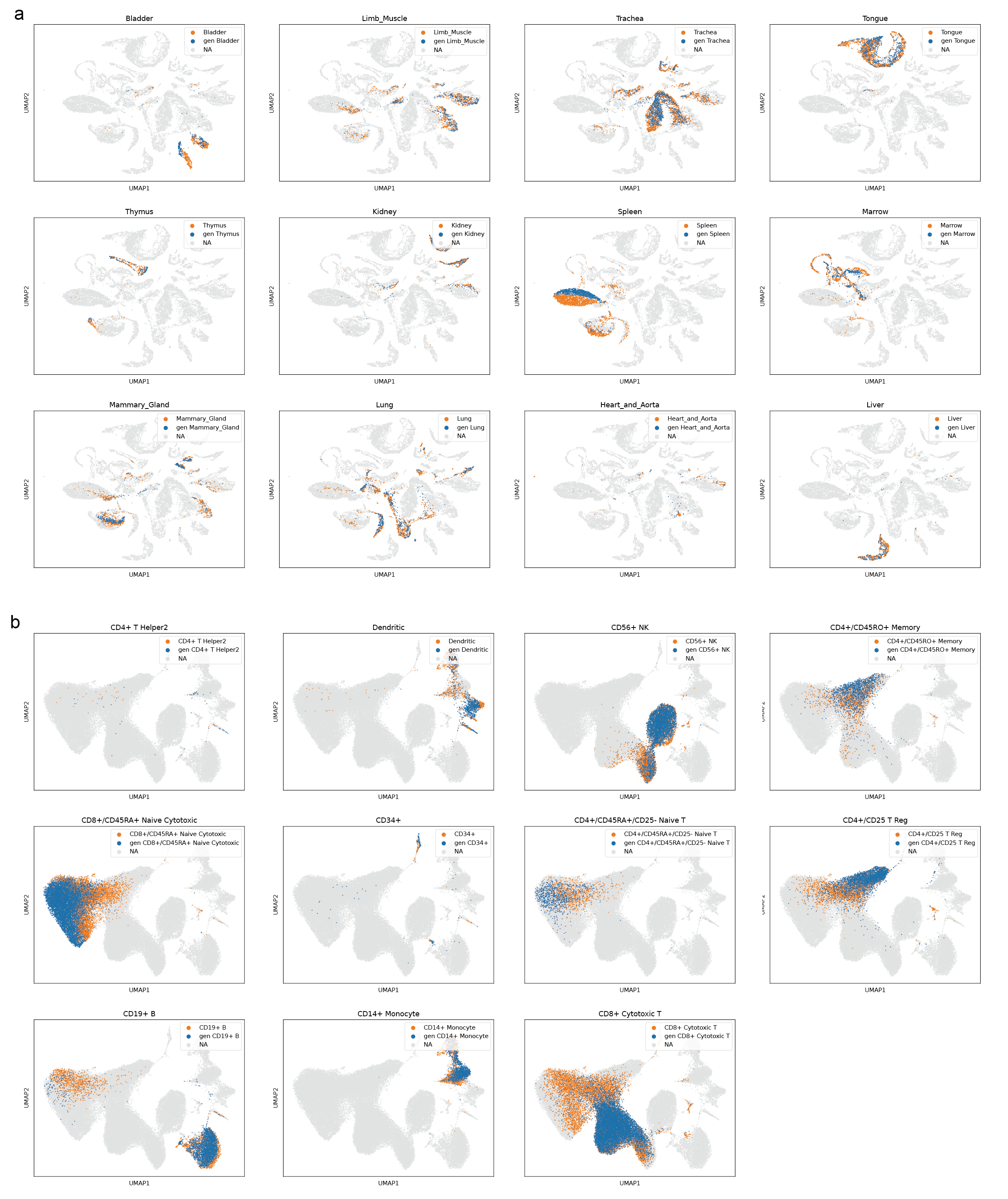
Figure S5: UMAP of conditionally generated cells. (a) The Tabular Muris dataset. (b) The PBMC68k dataset.

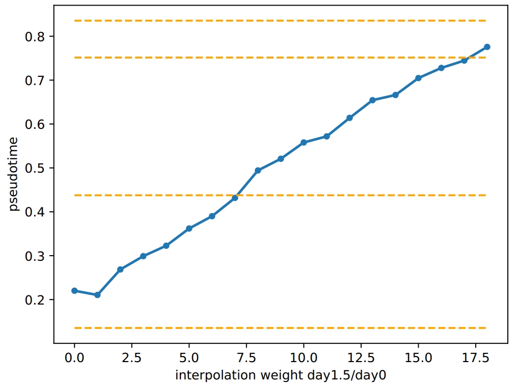
Figure S6: Pseudotime distance of generated states with different interpolation weights. Orange lines are the pseudotime of days 0, 0.5, 1, and 1.5 in the real data, from bottom to up.

References

- [1] Jovic, D. et al. Single-cell rna sequencing technologies and applications: A brief overview. Clinical and Translational Medicine 12, e694 (2022).
- [2] Gohil, S. H., Iorgulescu, J. B., Braun, D. A., Keskin, D. B. & Livak, K. J. Applying high-dimensional single-cell technologies to the analysis of cancer immunotherapy. Nature Reviews Clinical Oncology 18, 244–256 (2021).
- [3] Jiang, P. et al. Big data in basic and translational cancer research. Nature Reviews Cancer 22, 625–639 (2022).
- [4] Ke, M., Elshenawy, B., Sheldon, H., Arora, A. & Buffa, F. M. Single cell rna-sequencing: A powerful yet still challenging technology to study cellular heterogeneity. BioEssays 44, 2200084 (2022).
- [5] Suvà, M. L. & Tirosh, I. Single-cell rna sequencing in cancer: lessons learned and emerging challenges. Molecular cell 75, 7–12 (2019).
- [6] Greene, W. H. Accounting for excess zeros and sample selection in poisson and negative binomial regression models (1994).
- [7] Lindenbaum, O., Stanley, J., Wolf, G. & Krishnaswamy, S. Geometry based data generation. Advances in Neural Information Processing Systems 31 (2018).
- [8] Dibaeinia, P. & Sinha, S. Sergio: a single-cell expression simulator guided by gene regulatory networks. Cell systems 11, 252–271 (2020).
- [9] Li, W. V. & Li, J. J. A statistical simulator scdesign for rational scrna-seq experimental design. Bioinformatics 35, i41–i50 (2019).
- [10] Zappia, L., Phipson, B. & Oshlack, A. Splatter: simulation of single-cell rna sequencing data. Genome biology 18, 174 (2017).
- [11] Lopez, R., Gayoso, A. & Yosef, N. Enhancing scientific discoveries in molecular biology with deep generative models. Molecular systems biology 16, e9198 (2020).
- [12] Kingma, D. P. & Welling, M. Auto-encoding variational bayes. arXiv preprint arXiv:1312.6114 (2013).
- [13] Lopez, R., Regier, J., Cole, M. B., Jordan, M. I. & Yosef, N. Deep generative modeling for single-cell transcriptomics. Nature methods 15, 1053–1058 (2018).
- [14] Goodfellow, I. et al. Generative adversarial nets. Advances in neural information processing systems 27 (2014).
- [15] Marouf, M. et al. Realistic in silico generation and augmentation of single-cell rna-seq data using generative adversarial networks. Nature communications 11, 166 (2020).
- [16] Lall, S., Ray, S. & Bandyopadhyay, S. Lsh-gan enables in-silico generation of cells for small sample high dimensional scrna-seq data. Communications Biology 5, 577 (2022).
- [17] Xu, Y. et al. scigans: single-cell rna-seq imputation using generative adversarial networks. Nucleic acids research 48, e85–e85 (2020).
- [18] Brock, A., Donahue, J. & Simonyan, K. Large scale gan training for high fidelity natural image synthesis. arXiv preprint arXiv:1809.11096 (2018).
- [19] Ho, J., Jain, A. & Abbeel, P. Denoising diffusion probabilistic models. Advances in neural information processing systems 33, 6840–6851 (2020).
- [20] Yang, L. et al. Diffusion models: A comprehensive survey of methods and applications. ACM Computing Surveys (2022).
- [21] Cao, H. et al. A survey on generative diffusion model. arXiv preprint arXiv:2209.02646 (2022).
- [22] Dhariwal, P. & Nichol, A. Diffusion models beat gans on image synthesis. Advances in neural information processing systems 34, 8780–8794 (2021).
- [23] Song, J., Meng, C. & Ermon, S. Denoising diffusion implicit models. arXiv preprint arXiv:2010.02502 (2020).
- [24] Nichol, A. et al. Glide: Towards photorealistic image generation and editing with text-guided diffusion models. arXiv preprint arXiv:2112.10741 (2021).
- [25] Gretton, A., Borgwardt, K. M., Rasch, M. J., Schölkopf, B. & Smola, A. A kernel two-sample test. The Journal of Machine Learning Research 13, 723–773 (2012).
- [26] Haghverdi, L., Lun, A. T., Morgan, M. D. & Marioni, J. C. Batch effects in single-cell rna-sequencing data are corrected by matching mutual nearest neighbors. Nature biotechnology 36, 421–427 (2018).
- [27] Luecken, M. D. et al. Benchmarking atlas-level data integration in single-cell genomics. Nature methods 19, 41–50 (2022).
- [28] McInnes, L., Healy, J. & Melville, J. Umap: Uniform manifold approximation and projection for dimension reduction. arXiv preprint arXiv:1802.03426 (2018).
- [29] Domínguez Conde, C. et al. Cross-tissue immune cell analysis reveals tissue-specific features in humans. Science 376, eabl5197 (2022).
- [30] Zheng, G. X. et al. Massively parallel digital transcriptional profiling of single cells. Nature communications 8, 14049 (2017).
- [31] Schaum, N. et al. Single-cell transcriptomics of 20 mouse organs creates a tabula muris: The tabula muris consortium. Nature 562, 367 (2018).
- [32] Schiebinger, G. et al. Optimal-transport analysis of single-cell gene expression identifies developmental trajectories in reprogramming. Cell 176, 928–943 (2019).
- [33] Borrego, F., Masilamani, M., Marusina, A. I., Tang, X. & Coligan, J. E. The cd94/nkg2 family of receptors: from molecules and cells to clinical relevance. Immunologic research 35, 263–277 (2006).
- [34] Chu, P. G. & Arber, D. A. Cd79: a review. Applied Immunohistochemistry & Molecular Morphology 9, 97–106 (2001).
- [35] Lubberts, E. The il-23–il-17 axis in inflammatory arthritis. Nature Reviews Rheumatology 11, 415–429 (2015).
- [36] Schiopu, A., Cotoi, O. S. et al. S100a8 and s100a9: Damps at the crossroads between innate immunity, traditional risk factors, and cardiovascular disease. Mediators of inflammation 2013 (2013).
- [37] Haghverdi, L., Büttner, M., Wolf, F. A., Buettner, F. & Theis, F. J. Diffusion pseudotime robustly reconstructs lineage branching. Nature methods 13, 845–848 (2016).
- [38] Radford, A. et al. Learning transferable visual models from natural language supervision. In International conference on machine learning, 8748–8763 (PMLR, 2021).
- [39] Rombach, R., Blattmann, A., Lorenz, D., Esser, P. & Ommer, B. High-resolution image synthesis with latent diffusion models. In Proceedings of the IEEE/CVF conference on computer vision and pattern recognition, 10684–10695 (2022).