The Optimal Rate for Linear KB-splines and LKB-splines Approximation of High Dimensional Continuous Functions and its Application

Abstract

We propose a new approach for approximating functions in $C([0,1]^{d})$ via Kolmogorov superposition theorem (KST) based on the linear spline approximation of the K-outer function in Kolmogorov superposition representation. We improve the results in [27] by showing that the optimal approximation rate based on our proposed approach is $\mathcal{O}(\frac{1}{n^{2}})$, with $n$ being the number of knots over $[0,1]$, and the approximation constant increases linearly in $d$. We show that there is a dense subclass in $C([0,1]^{d})$ whose approximation can achieve such optimal rate, and the number of parameters needed in such approximation is at most $\mathcal{O}(nd)$. Moreover, for $d\geq 4$, we apply the tensor product spline denoising technique to smooth the KB-splines and get the corresponding LKB-splines. We use those LKB-splines as the basis to approximate functions for the cases when $d=4$ and $d=6$, which extends the results in [27] for $d=2$ and $d=3$. Based on the idea of pivotal data locations introduced in [27], we validate via numerical experiments that fewer than $\mathcal{O}(nd)$ function values are enough to achieve the approximation rates such as $\mathcal{O}(\frac{1}{n})$ or $\mathcal{O}(\frac{1}{n^{2}})$ based on the smoothness of the K-outer function. Finally, we demonstrate that our approach can be applied to numerically solving partial differential equation such as the Poisson equation with accurate approximation results.

Keywords: Kolmogorov superposition theorem, The curse of dimensionality, B-spline approximation, Tensor product splines denoising, The Poisson equation

Mathematics Subject Classification: 41A15, 41A63, 15A23

1 Introduction

Fast and effective computation of high dimensional function approximation has been at the research frontier since the advent of deep neural network, the bottleneck of having a good computational scheme is the issue of the curse of dimensionality. This issue has been a computational problem for many decades. A few advances have been made so far. One celebrated example of the Barron class of functions is proposed in [3, 4]. It is also well explained in [36]. The most recent results on neural network approximation of this class of functions can be found in [39] and [19]. Recently, the authors in [27] showed that there are subclasses of functions which are dense in $C([0,1]^{d})$ and can be approximated well by Kolmogorov superposition theorem without suffering the curse of dimensionality. Let us first recall the Kolmogorov superposition theorem (KST). We will introduce two versions of KST which appear in [22] and [30], respectively.

Theorem 1 (Kolmogorov Superposition Theorem — original version [22])

Let $f\in C([0,1]^{d})$, then there exists continuous functions $g_{q}:\mathbb{R}\to\mathbb{R}$ and $\phi_{qp}:[0,1]\to\mathbb{R}$ such that

$$f(x_{1},\cdots,x_{d})=\sum_{q=0}^{2d}g_{q}\left(\sum_{p=0}^{d}\phi_{qp}(x_{p})\right).$$ (1)

The significance of this surprising result can be summarized succinctly: Addition is the only continuous multivariate function. There have been many improvements of KST over the years. Lorentz [29] pointed out that the outer function $g_{q}$ can be chosen to be the same, while Sprecher [41] showed that one can take $\phi_{qp}=\lambda_{p}\phi_{q}$. Henkin [17] and Fridman [13] pointed out that the inner functions $\phi_{qp}$ can be chosen to be Hölder continuous with exponent $\alpha\in(0,1)$ and Lipschitz continuous, respectively. Sprecher [42, 43, 44, 45] also showed that inner functions can be replaced by one single inner function with an appropriate shift in its argument through the constructive form of KST. An excellent explanation of the history about the development of KST can be found in [34]. We now turn our attention to the Lorentz’s version of KST [30], which is more useful for the development of our approach.

Theorem 2 (Kolmogorov Superposition Theorem — Lorentz’s version [30])

There exist $0<\lambda_{p}\leq 1$, $p=1,\cdots,d$, and strictly increasing $\alpha$-Hölder continuous functions $\phi_{q}(x):[0,1]\to[0,1]$, $q=0,\cdots,2d$, with exponent $\alpha\in(0,1)$, such that for every $f\in C([0,1]^{d})$, there exists a continuous function $g\in C([0,d])$, such that

$$f(x_{1},\cdots,x_{d})=\sum_{q=0}^{2d}g\left(\sum_{p=1}^{d}\lambda_{p}\phi_{q}(x_{p})\right).$$ (2)

Some notable features of the representation formula (2) are the following. Firstly, there is only one outer function $g$ associated with $f$. Secondly, the number $2d+1$ in the summands can not be further reduced [35, 46]. Thirdly, the inner functions can not be chosen to be continuously differentiable [47, 48, 29].

The upshot for this representation is: for any continuous function $f\in C([0,1]^{d})$, there is a continuous function $g_{f}\in C([0,d])$ so that $f$ can be represented by $g_{f}$ via (2). Conversely, given any continuous function $g\in C([0,d])$, we can produce a continuous function $f_{g}\in C([0,1]^{d})$ by using the representation formula (2). Such a correspondence between $f$ and $g$ is one-to-one. Therefore we can use what we understand about univariate continuous functions to understand multivariate continuous functions.

It is worthy noting that KST also has some nice topology and machine learning interpretations. KST essentially established that all $d$ dimensional compact metrizable spaces can be embedded into $\mathbb{R}^{N}$ if and only if $N\geq 2d+1$. KST also guarantees that any continuous statistical or machine learning model, after a suitable embedding, is a sum of generalized additive models. There have been many generalizations and extensions of KST over the past few decades. Ostrand [35] showed that KST holds on compact metric spaces. Doss [10] and Demko [8] extended KST to $\mathbb{R}^{n}$ for unbounded and bounded continuous functions, respectively. Feng [12] generalized KST to locally compact and finite dimensional separable metric spaces.

It is straightforward to see that the representation formula (2) mimics the structure of a two-layer neural network where the inner and outer functions can be considered as activation functions. However, there have been debates over decades on whether such a representation via KST is useful. Girosi and Poggio [14] claimed that some degree of smoothness is required for inner and outer functions in order for the approximation to generalize and stabilize against noise. Lin and Unbehauen [28] made a similar conclusion by noting that all information carried by $f$ must be contained in the univariate function $g$ hence learning the latter is not any easier than learning the former. On the other hand, Køurkovà [20, 21] countered some of the criticisms from Girosi and Poggio by giving a constructive way to approximate the univariate outer function $g$ through linear combinations of the smooth sigmoid function. She also bounded the number of units needed for a desired approximation. This has in turn generated further interest in the study of neural network and approximation.

Indeed, KST has been actively studied which echoes the fast development of neural network computing [6, 32, 36]. Hecht-Nielsen [16] was among the first to draw a connection between KST and neural networks. This inspired much of the later works on universality of two-layer neural networks. However, Hecht-Nielsen was doubtful about the direct usefulness of this connection because no construction of the outer function was known then and he mentioned the possibility of learning the outer function from input-output examples. Later on, Igelnik and Parikh [18] proposed a neural network algorithm using spline functions to approximate both the inner and outer functions. More recently, active research has been conducted on neural network approximation via KST and achieves promising results [31, 15, 33, 38, 11]. However, these results are not directly based on the representation formula (2) and can be impractical to implement in practice. To the best of the authors’ knowledge, there is yet no approximation scheme that is directly based on KST and is straightforward to deploy in practice.

Recently, the authors in [27] introduced a class called K-Lipschitz continuous functions and proposed LKB-splines for approximating such functions with the rate $\mathcal{O}(1/n)$ and $\mathcal{O}(dn)$ terms of LKB-splines. Note that LKB-splines are a smooth version of KB-splines and the KB-splines are similar to the Kolmogorov spline network in the literature (cf. [18]). These KB-splines are very noisy and deemed useless. One of the significant features of the work [27] is the denoising of KB-splines. Therefore, LKB-splines in $\mathbb{R}^{d}$ with $d=2$ or $d=3$ are bivariate or trivariate spline functions (cf. [25]) after a denoising technique based on penalized least squares method (cf. [26]).

The main contribution of this paper is that it shows, via Kolmogorov superposition theorem (KST), that there is a dense subclass of continuous functions whose approximation rate is $\mathcal{O}(1/n^{2})$. Similar to [27], we also propose a new computational scheme based on tensor product spline denoising procedure to obtain LKB-splines in the setting $\mathbb{R}^{d}$ with $d=4$ and $d=6$, which can achieve the optimal approximation rate $\mathcal{O}(1/n^{2})$ with fewer than $\mathcal{O}(nd)$ number of LKB-splines and with fewer than $\mathcal{O}(nd)$ number of function values.

The remaining part of this paper is structured as follows. In section 2, we introduce a subclass of continuous functions, called K-Hölder class. We show that this class is dense in $C([0,1]^{d})$ by showing a subclass of this class is dense. We also introduce linear KB-spline functions based on the linear approximation of the K-outer function and show that there is a dense subclass of $C([0,1]^{d})$ which can be approximated by using KB-splines with the optimal approximation rate $\mathcal{O}(1/n^{2})$. In section 3, we introduce a tensor product spline denoising method to smooth the KB-spline basis and get the corresponding LKB-spline basis for our approximation scheme. In section 4, we demonstrate the numerical results for function approximation as $d=4$ and $d=6$ by using linear LKB-splines as basis. In section 5, we show the numerical method of solving Poisson equation based on LKB-splines as one application of our approach. Finally, in section 6, we conclude the paper and point out some future research directions.

2 K-Hölder class

We will consider a general class of continuous functions called K-Hölder class. Let us call the function $g$ and $\phi_{q}$ in (2) the K-outer function and K-inner function respectively. For each continuous function $f\in C([0,1]^{d})$, let

$$K_{\beta}:=\{f:\hbox{ K-outer function $g$ is $\beta$-Hölder continuous with exponent $0<\beta<1$ }\}$$ (3)

be the class of K-Hölder continuous functions with exponent $\beta$. Recall that we say a function $f$ is in $C^{0,\alpha}$ if

$$\sup_{x,y\in[0,d]}\frac{|f(x)-f(y)|}{|x-y|^{\alpha}}<\infty.$$ (4)

One can easily show

Theorem 3

Under the KST representation (2). Suppose $f\in K_{\beta}$, then $f\in C^{0,\alpha\beta}$.

• Proof. Suppose $\mathbf{x},\mathbf{y}\in[0,1]^{d}$, and $(x_{1},\cdots,x_{d})=\mathbf{x}\neq\mathbf{y}=(y_{1},\cdots,y_{d})$. Then

  $$\left|f(\mathbf{x})-f(\mathbf{y})\right| =\left|\sum_{q=0}^{2d}g\left(\sum_{i=1}^{d}\lambda_{i}\phi_{q}(x_{i})\right)-\sum_{q=0}^{2d}g\left(\sum_{i=1}^{d}\lambda_{i}\phi_{q}(y_{i})\right)\right|$$

  $$\leq\sum_{q=0}^{2d}\left|g\left(\sum_{i=1}^{d}\lambda_{i}\phi_{q}(x_{i})\right)-g\left(\sum_{i=1}^{d}\lambda_{i}\phi_{q}(y_{i})\right)\right|$$

  $$\leq\sum_{q=0}^{2d}C_{1}\left|\sum_{i=1}^{d}\lambda_{i}\phi_{q}(x_{i})-\sum_{i=1}^{d}\lambda_{i}\phi_{q}(y_{i})\right|^{\beta}\leq\sum_{i=0}^{2d}C_{1}\sum_{i=1}^{d}\lambda_{i}^{\beta}\left|\phi_{q}(x_{i})-\phi_{q}(y_{i})\right|^{\beta}$$

  $$\leq\sum_{q=0}^{2d}C_{1}\sum_{i=1}^{d}\lambda_{i}^{\beta}C_{2}^{\beta}|x_{i}-y_{i}|^{\alpha\beta}\leq(2d+1)C_{1}C_{2}^{\beta}\sum_{i=1}^{d}|x_{i}-y_{i}|^{\alpha\beta}.$$

  This completes the proof. $\Box$

Now let us introduce two important subclasses of K-Hölder continuous functions: K-polynomials and KB-splines.

2.1 K-polynomials and K-monomials

Let us define the K-polynomial as

$$Kp_{n}(x_{1},\cdots,x_{d})=\sum_{q=0}^{2d+1}p_{n}\left(\sum_{i=1}^{d}\lambda_{i}\phi_{q}(x_{i})\right),$$ (5)

where the function $p_{n}$ is a univariate polynomial. We call it a K-monomial if $p_{n}(t):=t^{n}$, $n\geq 0$. Figure 1 shows some plots of different K-monomials with and without using the denoising/smoothing technique described in [27]. The significance of K-monomials are that the $span\{Kp_{n}\}_{n\geq 0}$ are dense in $C([0,1]^{d})$. Let us call this result the K-Weierstrass theorem.

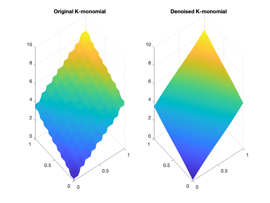
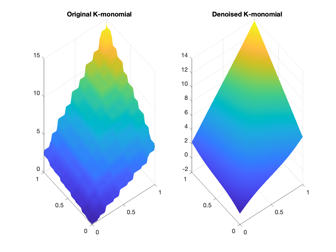
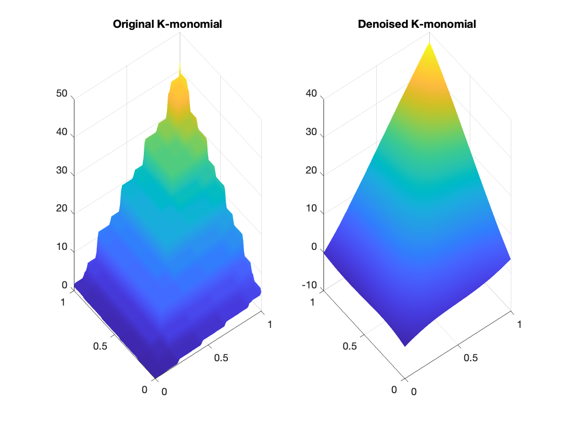
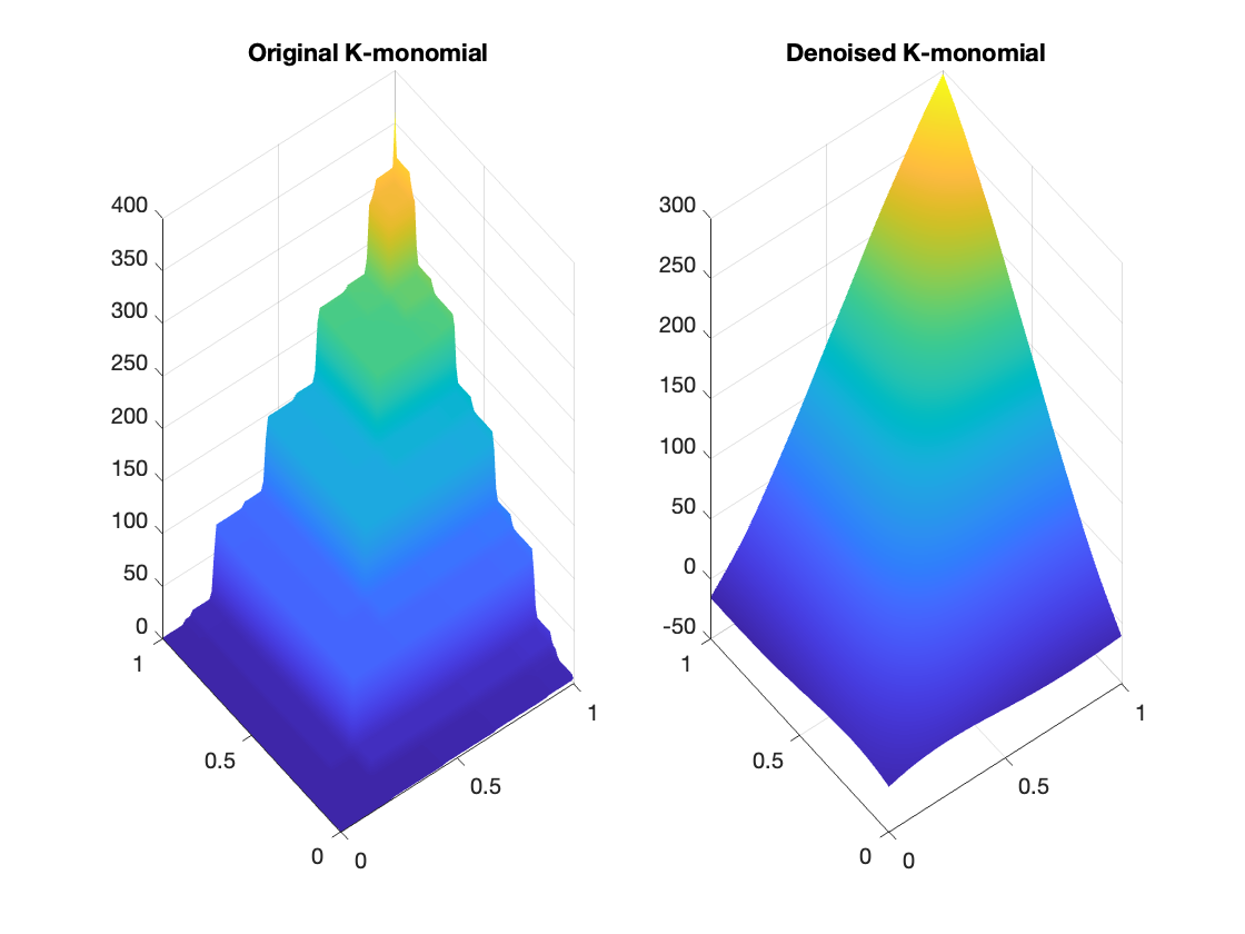
Figure 1: Examples of K-monomials (Top Row: $p_{n}(x)=x,x^{2}$. Bottom Row: $p_{n}(x)=x^{4},x^{8}$).

Theorem 4 (K-Weierstrass Theorem)

For any $f\in C([0,1]^{d})$ and for any $\epsilon>0$, there exists $K\in span\{Kp_{n}\}_{n\geq 0}$ such that

$$\|f-K\|_{\infty}\leq\epsilon.$$ (6)

• Proof. By Kolmogorov superposition theorem, we can write $f(x_{1},\cdots,x_{d})=\sum_{q=0}^{2d+1}g\left(\sum_{i=1}^{d}\lambda_{i}\phi_{q}(x_{i})\right)$. By Weierstrass approximation theorem, there exists a polynomial $p$ such that $|p(t)-g(t)|\leq\frac{\epsilon}{2d+1}$ for all $t\in[0,d]$. Letting $K(x_{1},\cdots,x_{d})=\sum_{q=0}^{2d+1}p\left(\sum_{i=1}^{d}\lambda_{i}\phi_{q}(x_{i})\right)\in span\{Kp_{n}\}_{n\geq 0}$, we have

  $$|f(x_{1},\cdots,x_{d})-K(x_{1},\cdots,x_{d})| =\left|\sum_{q=0}^{2d+1}g\left(\sum_{i=1}^{d}\lambda_{i}\phi_{q}(x_{i})\right)-\sum_{q=0}^{2d+1}p\left(\sum_{i=1}^{d}\lambda_{i}\phi_{q}(x_{i})\right)\right|$$

  $$\leq\sum_{q=0}^{2d+1}\left|g\left(\sum_{i=1}^{d}\lambda_{i}\phi_{q}(x_{i})\right)-p\left(\sum_{i=1}^{d}\lambda_{i}\phi_{q}(x_{i})\right)\right|$$

  $$\leq(2d+1)\cdot\frac{\epsilon}{(2d+1)}=\epsilon.$$

  This completes the proof. $\Box$

Remark 1

There are many $f\in C([0,1]^{d})$ are K-Hölder continuous. Indeed, in addition to K-polynomials, we can use trigonmetric functions as K-outer function g to define high dimensional continuous functions called K-trigonometric functions via (2). Similarly, we can have $K$-exponential functions, $K$-logarithmic functions, etc,. In fact, any univariate Hölder continuous function $g$ gives a $K$-Hölder continuous function $f$ via Kolmogorov representation formula by using Theorem 2. Because these univariate functions $g$ are of Hölder continuous, their corresponding $f$ are in the K-Hölder continuous class.

2.2 Linear KB-splines and LKB-splines

It is well known that linear spline function can be represented in terms of linear combination of ReLU functions and vice versa, see, e.g. [7], and [9]. Let $S^{0}_{1}(\triangle)$ be the space of all continuous linear splines over the partition $\triangle=\{0=t_{0}<t_{1}<\cdots<t_{n}=1\}$ with $|\triangle|=\max_{i}|t_{i}-t_{i-1}|$. For univariate function $f$, let $\omega(f,h):=\sup_{|x-y|\leq h}|f(x)-f(y)|$ be its modulus of continuity. From standard approximation theory (c.f. [37]), we know that

Lemma 1

Suppose $f\in C([0,1])$, let $\triangle$ be a partition over $[0,1]$ with $n$ knots. Then there exists a $L_{f}\in S^{0}_{1}(\triangle)$ such that

$$\|f-L_{f}\|_{\infty}\leq\begin{cases}\omega(f,\frac{1}{n}),\quad\text{if}\quad f\in C([0,1]),\\ \frac{1}{2n}\|f^{\prime}\|_{\infty},\quad\text{if}\quad f\in C^{1}([0,1]),\\ \frac{1}{8n^{2}}\|f^{\prime\prime}\|_{\infty},\quad\text{if}\quad f\in C^{2}([0,1]).\end{cases}$$ (7)

Remark 2

Note that even if we can further increase the smoothness of function $f$, the approximation rate is not getting better. In order to achieve a better approximation rate for those $f$ with higher order smoothness, one has to use a higher degree splines. Therefore, for linear spline approximation, $\mathcal{O}(\frac{1}{n^{2}})$ is the optimal approximation rate.

For $f\in C([0,1]^{d})$, we would like to apply Lemma 1 for approximating the K-outer function $g$, and hence approximating $f$ via the representation formula (2). For this purpose, let us define the linear KB-splines of $f$ as

$$KB(f)_{n}(x_{1},\cdots,x_{d}):=\sum_{q=0}^{2d+1}L_{g}\left(\sum_{i=1}^{d}\lambda_{i}\phi_{q}(x_{i})\right),$$ (8)

where $L_{g}$ is chosen to be a linear spline interpolation of the K-outer function $g\in C([0,d])$ with uniform partition of $nd$ knots, i.e., $|\triangle|=\frac{1}{n}$. Then by Theorem 2 and Lemma 1, we have

Theorem 5

Suppose $f\in C([0,1]^{d})$. Then

$$\|f-KB(f)_{n}\|_{\infty}\leq\begin{cases}(2d+1)\omega(g,\frac{1}{n}),\quad\text{if}\quad g\in C([0,d]),\\ \frac{2d+1}{2n}\|g^{\prime}\|_{\infty},\quad\text{if}\quad g\in C^{1}([0,d]),\\ \frac{2d+1}{8n^{2}}\|g^{\prime\prime}\|_{\infty},\quad\text{if}\quad g\in C^{2}([0,d]).\end{cases}$$ (9)

• Proof. We only show the proof for the case $g\in C^{2}([0,d])$, and the other two cases are similar. For any $\mathbf{x}=(x_{1},\cdots,x_{d})$, we have

  $$\left|f(\mathbf{x})-KB(f)_{n}(\mathbf{x})\right| =\left|\sum_{q=0}^{2d+1}g\left(\sum_{i=1}^{d}\lambda_{i}\phi_{q}(x_{i})\right)-\sum_{q=0}^{2d+1}L_{g}\left(\sum_{i=1}^{d}\lambda_{i}\phi_{q}(x_{i})\right)\right|$$

  $$\leq\sum_{q=0}^{2d+1}\left|g\left(\sum_{i=1}^{d}\lambda_{i}\phi_{q}(x_{i})\right)-L_{g}\left(\sum_{i=1}^{d}\lambda_{i}\phi_{q}(x_{i})\right)\right|\leq\frac{2d+1}{8n^{2}}\|g^{\prime\prime}\|_{\infty}.$$

  This completes the proof. $\Box$

Theorem 5 immediately shows linear KB-splines are dense in $C([0,1]^{d})$. More importantly, the approximation rate of linear KB-splines is independent of dimension $d$ while the approximation constant is linearly dependent on $d$. Therefore we conclude that the approximation of high dimensional continuous function $f$ does not suffer from the curse of dimensionality for a subclass of $C([0,1]^{d})$, i.e., those $f$ whose $K$-outer function $g\in C^{1}([0,d])$ or $g\in C^{2}([0,d])$. Such a subclass is dense because $C^{1}([0,d])$ and $C^{2}([0,d])$ are dense in $C([0,d])$. In fact, there are enormous choices of such $g$. For example, we can choose $g$ to be polynomial functions, trigonometric functions, exponential functions, etc,.

Furthermore, let us recall the linear KB-splines basis functions defined in [27]. Let $\triangle_{n}=\{0=t_{1}<t_{2}<\cdots<t_{dn}<d\}$ be a uniform partition of interval $[0,d]$, and $b_{n,i}(t),i=1,\cdots,dn$ be the standard univariate linear B-splines, we define the linear KB-spline (basis) functions as

$$KB_{n,j}(x_{1},\cdots,x_{d}):=\sum_{q=0}^{2d}b_{n,j}\left(\sum_{i=1}^{d}\lambda_{i}\phi_{q}(x_{i})\right),j=1,\cdots,dn.$$ (10)

In [27], we showed that these $KB_{n,j}$ have several nice properties, e.g. the partition of unity, linear independence, and denseness in $C([0,1]^{d})$. Therefore we can treat $KB_{n,j}$ as basis functions for approximating $f\in C([0,1]^{d})$. However, since there are only $\mathcal{O}(dn)$ number of $KB_{n,j}$ basis functions, the amount of information each basis $KB_{n,j}$ carries is much more than the information carried by each of the $\mathcal{O}(n^{d})$ basis in the usual tensor product approximation or polynomial approximation. The basis $KB_{n,j}$ can behave very wildly, for example, they are not differentiable, and hence can not be directly used for approximating $f$. For $d=2$ and $d=3$, we apply a spline denoising technique as introduced in [27] to smooth the KB-splines and get the corresponding LKB-splines. We leave the details for construction of LKB-splines to [27]. For dimension $d\geq 4$, we need to apply tensor product of such denoising technique as introduced in the next section.

3 Tensor Product Approximation and Denoising

Let us first recall the approximation based on tensor product of Bernstein polynomial, which is well-known in the literature. We review them in order to explain the computation of tensor product splines for denoising in the later subsection.

3.1 Tensor product approximation of Bernstein polynomial

Suppose $f\in C([0,1])$, we define the Bernstein operator of degree $n$ on $f$ as

$$B_{n}f(x):=\sum_{i=0}^{n}f\left(\frac{i}{n}\right)B_{n,i}(x)$$ (11)

where $B_{n,i}=\binom{n}{i}x^{i}(1-x)^{n-i}$ is the Bernstein basis polynomial. From standard approximation theory (c.f. [37]), we know

Lemma 2

Suppose $f\in C^{2}([0,1])$. Then

$$\|f-B_{n}f\|_{\infty}\leq\frac{1}{8n}\|f^{\prime\prime}\|_{\infty}.$$ (12)

In general, for $f\in C([0,1]^{d})$, we can define

$$B_{n_{1},\cdots,n_{d}}f(x_{1},\cdots,x_{d}):=\sum_{i_{1}=0}^{n_{1}}\cdots\sum_{i_{d}=0}^{n_{d}}f\left(\frac{i_{1}}{n_{1}},\cdots,\frac{i_{d}}{n_{d}}\right)B_{n_{1},i_{1}}(x_{1})\cdots B_{n_{d},i_{d}}(x_{d}).$$ (13)

By applying Lemma 2 and and a chain of triangle inequalities argument, it is not hard to establish the following result. We leave its proof to the interested readers.

Lemma 3

Suppose $f\in C^{2}([0,1]^{d})$ for integer $d\geq 1$. Then

$$\|f-B_{n,\cdots,n}f\|_{\infty}\leq\frac{d}{8n}|f^{\prime\prime}|_{2,\infty},$$ (14)

where $|f|_{2,\infty}=\max_{i_{1}+\cdots+i_{d}=2}\|D_{x_{1}}^{i_{1}}\cdots D_{x_{d}}^{i_{d}}f\|_{\infty}$.

3.2 Tensor product of spline denoising

As mentioned before, the linear KB-splines obtained via (10) can behave wildly, therefore may not be directly useful for approximation. We would like to smooth/denoise them so that they will be useful. For self-containedness, let us introduce the ideas of spline denoising and tensor product spline denoising. For convenience, we base our discussion on the bivariate splines. Let us first recall bivariate spline spaces. For a triangulation $\triangle$ of $[0,1]^{2}$, for any degree $d\geq 1$ and smoothness $r\geq 1$ with $r<d$, let

$$S^{r}_{d}(\triangle)=\{s\in C^{r}([0,1]^{2}):s|_{T}\in\mathbb{P}_{d},T\in\triangle\}$$ (15)

be the spline space of degree $d$ and smoothness $r$ with $d>r$. We refer to [25] for a theoretical detail and [2] and [24] for a computational detail of multivariate splines. For convenience, we can write a spline function

$$s(x,y)=\sum_{i=1}^{m}c_{i}b_{i}(x,y)\in S^{r}_{d}(\triangle),$$ (16)

where $c_{i}$’s are the spline coefficients, $b_{i}(\cdot,\cdot)$ are bivariate basis splines with degree $d$ and smoothness $r$, and $m$ is the dimension of the bivariate spline space. Note that the computation of $b_{i}(x,y)$ is not easy at all. We adopt the approach in [2].

For a given data set $\{(x_{i},y_{i},z_{i}),i=1,\cdots,N\}$ with data locations $(x_{i},y_{i})\in[0,1]^{2}$ and noisy data values $z_{i}$, the penalized least squares method (cf. [23] and [26]) of bivariate spline denoising is to find

$$\min_{s\in S^{r}_{d}(\triangle)}\sum_{i=1,\cdots,N}\left|s(x_{i},y_{i})-z_{i}\right|^{2}+\lambda{\cal E}_{2}(s)$$ (17)

for some fixed constant $\lambda\approx 1$, where ${\cal E}_{2}(s)$ is the thin-plate energy functional defined as

$${\cal E}_{2}(s):=\int_{[0,1]^{2}}\left|\frac{\partial^{2}}{\partial x^{2}}s\right|^{2}+2\left|\frac{\partial^{2}}{\partial x\partial y}s\right|^{2}+\left|\frac{\partial^{2}}{\partial y^{2}}s\right|^{2}.$$ (18)

It is well-known that this approach can be used for smoothing noisy data. This is the denoising technique we have used in [27] to generate linear LKB-splines, which are much smoother and nicer. Some examples of generated linear LKB-splines are shown in Figure 2.

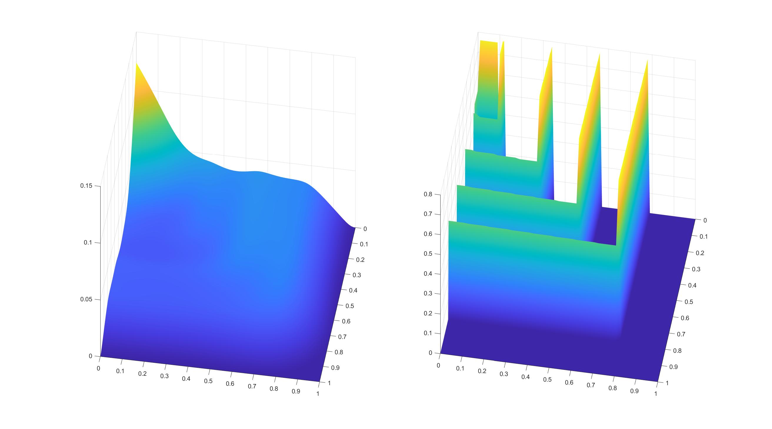
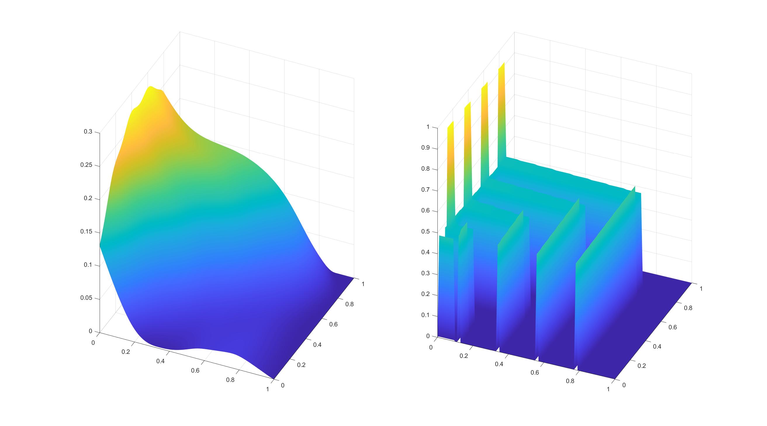
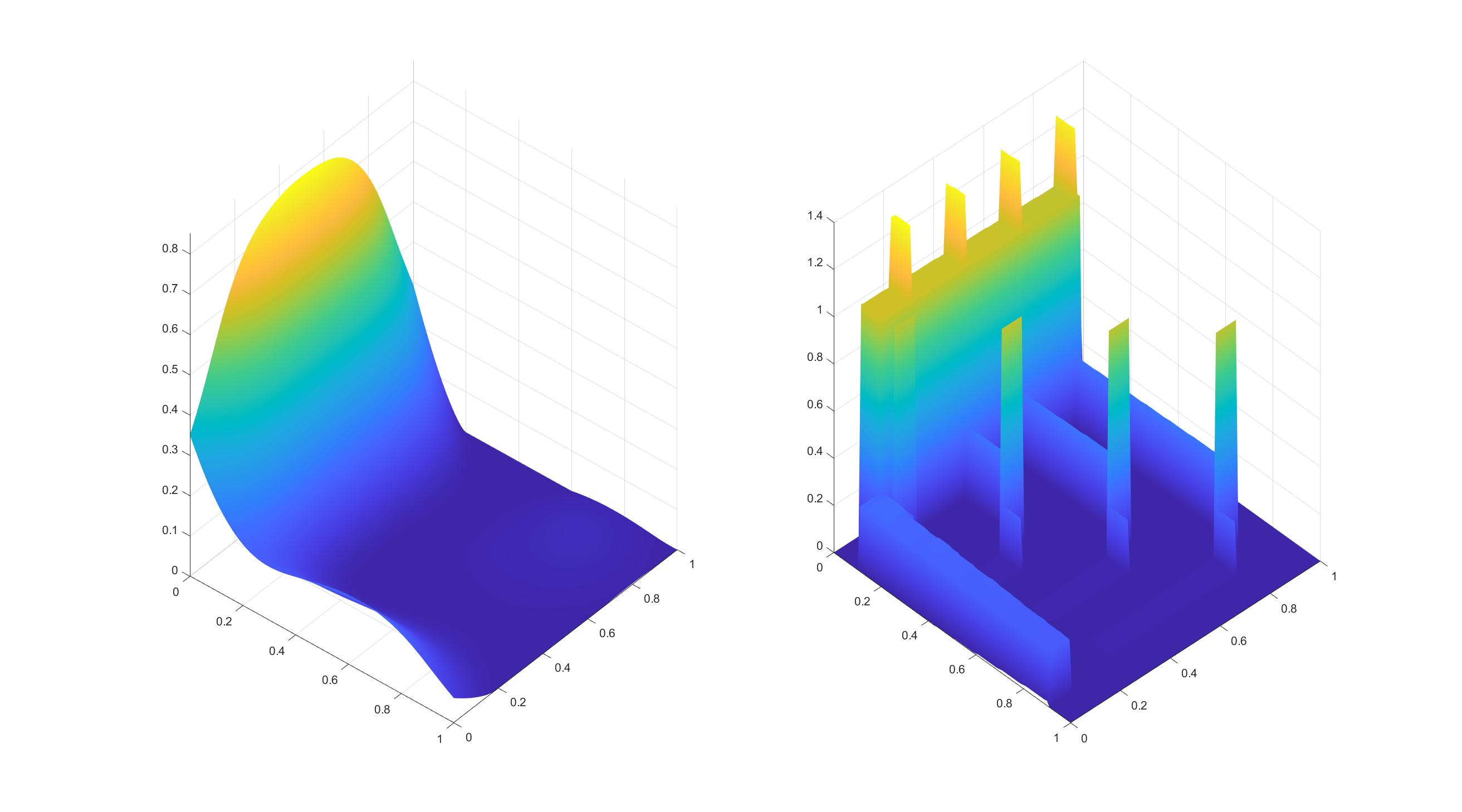
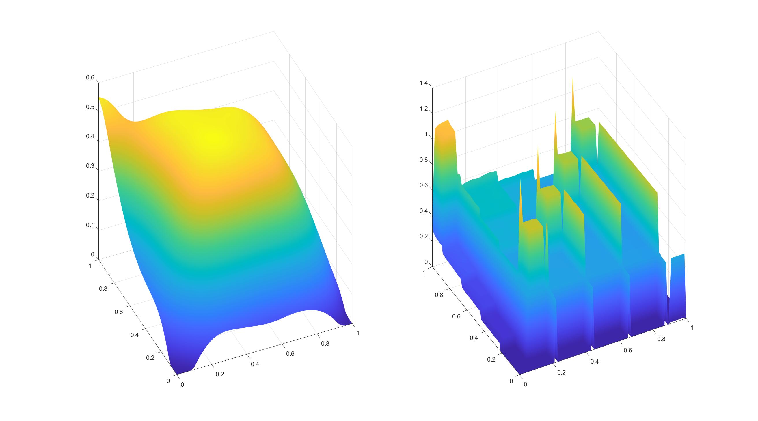
Figure 2: Some examples of linear LKB-splines (the first and third columns) which are the smoothed version of the corresponding linear KB-splines (the second and fourth columns).

Now let us explain the idea of tensor product spline based denoising method for smoothing noisy KB-splines. For convenience, let us consider the case $d=4$, the similar arguements can be applied to a general $d$. See [5] for the general case for tensor product splines for data interpolation. For the rest of the discussion, we shall consider the tensor product the bivariate spline space ${\cal S}:=S^{r}_{d}(\triangle)\times S^{r}_{d}(\triangle)$.

For a given data set $\{(x_{i},y_{i},u_{j},v_{j},z_{i,j}),i,j=1,\cdots,N\}$ with data locations $(x_{i},y_{i},u_{j},v_{j})\in[0,1]^{2}\times[0,1]^{2}$ and noisy data values $z_{i,j}$, we can write a spline function

$$s(x,y,u,v)=\sum_{i=1}^{m_{1}}\sum_{j=1}^{m_{2}}c_{ij}b_{i}(x,y)b_{j}(u,v)\in{\cal S},$$ (19)

where $c_{ij}$’s are the spline coefficients, $b_{i}(\cdot,\cdot)$ are bivariate splines with degree $d$ and smoothness $r$, and $m_{1},m_{2}$ are the dimensions of the bivariate spline spaces. The penalized least squares method of tensor product bivariate spline denoising is to find the spline coefficients $c_{ij}$ which solves

$$\min_{s\in{\cal S}}\sum_{i,j=1,\cdots,N}|s(x_{i},y_{i},u_{j},v_{j})-z_{ij}|^{2}+\lambda{\cal E}_{2\times 2}(s)$$ (20)

with $r>0,d>0,\lambda\approx 1$ are hyperparameters, and ${\cal E}_{2\times 2}(s)$ is defined as

$${\cal E}_{2\times 2}(s) :=\int_{[0,1]^{2}}\left(\int_{[0,1]^{2}}\left|\frac{\partial^{2}}{\partial x^{2}}s\right|^{2}+2\left|\frac{\partial^{2}}{\partial x\partial y}s\right|^{2}+\left|\frac{\partial^{2}}{\partial y^{2}}s\right|^{2}dxdy\right)dudv$$ (21)

$$+\int_{[0,1]^{2}}\left(\int_{[0,1]^{2}}\left|\frac{\partial^{2}}{\partial u^{2}}s\right|^{2}+2\left|\frac{\partial^{2}}{\partial u\partial v}s\right|^{2}+\left|\frac{\partial^{2}}{\partial v^{2}}s\right|^{2}dudv\right)dxdy.$$

Let us explain next the computational procedure for finding the spline coefficients $c_{ij}$ based on a two-stage bivariate spline denoising scheme. Recall that tensor product splines for data interpolation were explained in [5]. We extend its ideas to data denoising. For a given data set $\{(x_{i},y_{i},u_{j},v_{j},z_{i,j}),i,j=1,\cdots,N\}$ with data locations $(x_{i},y_{i})\in[0,1]^{2}$ and $(u_{j},v_{j})\in[0,1]^{2}$ and noised data values $z_{i,j}$, $i,j=1,\cdots,N$, we can write

$$s(x,y,u,v)=\sum_{i=1}^{m_{1}}\sum_{j=1}^{m_{2}}c_{ij}b_{j}(u,v)b_{i}(x,y).$$ (22)

Suppose our data is equally-spaced over $[0,1]^{2}\times[0,1]^{2}$, i.e., $N=m_{1}=m_{2}$. Let us denote $d_{i}(u,v)=\sum_{j=1}^{m_{2}}c_{ij}b_{j}(u,v)$, then we can write equation (22) as $s(x,y,u,v)=\sum_{i=1}^{m_{1}}d_{i}(u,v)b_{i}(x,y)$. For fixed $(u_{k},v_{k})$, $k=1,\cdots,N$, write $d_{i}(u_{k},v_{k})=d_{ik}$ for all $i=1,\cdots,m_{1}$. For each fixed $k$, we can find the intermediate spline coefficients $d_{ik}$ via (17) by letting

$$s(x_{\ell},y_{\ell})_{k}:=s(x_{\ell},y_{\ell},u_{k},v_{k})=\sum_{i=1}^{m_{1}}d_{ik}b_{i}(x_{\ell},y_{\ell})$$ (23)

for $\ell=1,\cdots,N$. Once we have $d_{ik}$, then for each fixed $i$, we can find the spline coefficients $c_{ij}$ via (17) by letting

$$s(u_{k},v_{k}):=d_{ik}=\sum_{j=1}^{m_{2}}c_{ij}b_{j}(u_{k},v_{k})$$ (24)

for $k=1,\cdots,N$.

The advantage of tensor product spline denoising is its computational efficiency. If we directly solve the penalized least squares problem (20) for the coefficients $c_{ij}$ without using this tensor product approach, then the matrix size associated in (22) is $N^{2}\times m_{1}m_{2}$. Hence, solving it directly requires the computation complexity $\mathcal{O}(m_{1}^{2}m_{2}^{2}N^{2})$. However, if we solve it by using tensor product via (23) and (24), then we only need to solve $N$ systems whose matrix size is of $N\times m_{1}$ and another $N$ systems whose matrix size is of $N\times m_{2}$. Therefore the computational complexity for solving them directly requires $\mathcal{O}(Nm_{1}^{2}N+Nm_{2}^{2}N)=\mathcal{O}((m_{1}^{2}+m_{2}^{2})N^{2})$. If we use large degree $d$ and high smoothness $r\geq 1$ for denoising, then $m_{1}^{2}+m_{2}^{2}\ll m_{1}^{2}m_{2}^{2}$. Therefore, the computational cost for the two-stage tensor product denoising technique is much less than the direct denosing technique. This is why we adopt the tensor product spline denosing method. For the general case $d>4$, we can easily extend this idea to have a multi-stage denoising scheme. We leave out the details here.

For each high dimensional linear KB-spline obtained via (10), we can apply such a computational scheme to solve (20) and obtain the corresponding high dimensional linear LKB-spline, which is useful for approximation. We will use these linear LKB-splines as basis for high dimensional function approximation. Numerical results will be discussed in the following sections.

4 Experiments for LKB-spline based Approximation

Let us present the numerical results for function approximation in $\mathbb{R}^{d}$ with $d=4$ and $d=6$ based on the linear LKB-splines obtained via the computation procedure described in the previous section.

In 4D, we sampled $11^{4}$ equally-spaced data across $[0,1]^{4}$ and fit discrete least squares (DLS) approximation of a continuous function $f$ with 4D linear LKB-spline as basis, and we check the RMSEs based on $26^{4}$ equally-spaced data across $[0,1]^{4}$. The following 10 testing functions across different families of continuous functions are used to check the approximation accuracy.

$$f_{1} = (1+2x+3y+4u+5v)/15;$$

$$f_{2} = (x^{2}+y^{2}+u^{2}+v^{2})/4;$$

$$f_{3} = (x^{4}+y^{4}+u^{4}+v^{4})/4;$$

$$f_{4} = (\sin(x)\exp(y)+\cos(x)\exp(u)+\sin(x)\exp(v))/(3\exp(1));$$

$$f_{5} = 1/(1+x^{2}+y^{2}+u^{2}+v^{2});$$

$$f_{6} = \sin(\pi x)\sin(\pi y)\sin(\pi u)\sin(\pi v);$$

$$f_{7} = (\sin(\pi(x^{2}+y^{2}+u^{2}+v^{2}))+1)/2;$$

$$f_{8} = \exp(-x^{2}-y^{2}-u^{2}-v^{2});$$

$$f_{9} = \max(x-0.5)\max(y-0.5)\max(u-0.5)\max(v-0.5);$$

$$f_{10} = \max(x+y+u+v-2,0);$$

In 6D, we sampled $6^{6}$ equally-spaced data across $[0,1]^{6}$ and fit DLS approximation of a continuous function $f$ with 6D linear LKB-splines, and we check the RMSEs based on $11^{6}$ equally-spaced data across $[0,1]^{6}$. The following 10 testing functions across different families of continuous functions are used to check the approximation accuracy.

$$f_{1} = (1+2x+3y+4z+5u+6v+7w)/28;$$

$$f_{2} = (x^{2}+y^{2}+z^{2}+u^{2}+v^{2}+w^{2})/6;$$

$$f_{3} = (x^{3}y^{3}+x^{3}z^{3}+y^{3}z^{3}+x^{3}u^{3}+u^{3}v^{3}+v^{3}w^{3})/6;$$

$$f_{4} = (\sin(x)e^{y}+\cos(x)e^{z}+\sin(x)e^{u}+\cos(y)e^{v}+\sin(x)e^{w})/(5e);$$

$$f_{5} = 1/(1+x^{2}+y^{2}+z^{2}+u^{2}+v^{2}+w^{2});$$

$$f_{6} = \sin(\pi x)\sin(\pi y)\sin(\pi z)\sin(\pi u)\sin(\pi v)\sin(\pi w);$$

$$f_{7} = (\sin(\pi(x^{2}+y^{2}+z^{2}+u^{2}+v^{2}+w^{2}))+1)/2;$$

$$f_{8} = \exp(-x^{2}-y^{2}-z^{2}-u^{2}-v^{2}-w^{2});$$

$$f_{9} = \max(x-0.5)\max(y-0.5)\max(z-0.5)\max(u-0.5)\max(v-0.5)\max(w-0.5);$$

$$f_{10} = \max(x+y+z+u+v+w-3,0);$$

Table 1: RMSEs (computed based on $26^{4}$ equally-spaced locations) of the DLS fitting based $11^{4}$ equally-space sampled data and pivotal location in 4D.

	$n=100$		$n=300$		$n=1000$
# Sampled Data	$11^{4}$	$128$	$11^{4}$	$241$	$11^{4}$	$531$
$f_{1}$	3.06e-04	8.90e-04	6.02e-05	4.24e-04	2.79e-06	9.86e-06
$f_{2}$	9.70e-04	2.75e-03	4.35e-04	1.63e-03	2.66e-04	5.85e-04
$f_{3}$	4.00e-03	1.13e-02	1.87e-03	6.88e-03	1.12e-03	2.32e-03
$f_{4}$	5.86e-04	1.88e-03	3.23e-04	1.45e-03	1.62e-04	4.31e-04
$f_{5}$	1.39e-03	3.63e-03	4.76e-04	1.80e-03	2.67e-04	7.07e-04
$f_{6}$	3.40e-02	1.07e-01	1.33e-02	7.80e-02	3.96e-03	2.24e-02
$f_{7}$	9.75e-02	3.07e-01	4.13e-02	1.96e-01	1.57e-02	5.40e-02
$f_{8}$	1.54e-03	3.78e-03	6.28e-04	2.55e-03	3.58e-04	8.85e-04
$f_{9}$	3.51e-04	1.29e-03	1.80e-04	1.56e-03	1.03e-04	5.59e-04
$f_{10}$	2.53e-02	5.32e-02	1.96e-02	8.25e-02	1.40e-02	3.45e-02

Table 2: RMSEs (computed based on $11^{6}$ equally-spaced locations) of the DLS fitting based $6^{6}$ equally-space sampled data and pivotal location in 6D.

	$n=20$		$n=40$		$n=120$
# Sampled Data	$6^{6}$	$13$	$6^{6}$	$24$	$6^{6}$	$70$
$f_{1}$	5.09e-02	7.81e-02	3.03e-02	5.52e-02	7.78e-03	3.61e-02
$f_{2}$	4.56e-02	1.31e-01	4.09e-02	8.30e-02	1.73e-02	5.31e-02
$f_{3}$	9.70e-02	1.29e-01	5.26e-02	8.39e-02	2.85e-02	5.09e-02
$f_{4}$	7.50e-02	2.50e-01	7.27e-02	1.50e-01	3.59e-02	1.23e-01
$f_{5}$	5.44e-02	1.88e-01	4.98e-02	1.22e-01	2.72e-02	7.25e-02
$f_{6}$	3.95e-02	8.07e-02	3.55e-02	6.14e-02	1.64e-02	4.45e-02
$f_{7}$	2.50e-02	8.71e-02	2.40e-02	6.46e-02	9.08e-03	3.94e-02
$f_{8}$	8.84e-02	9.39e-02	6.83e-02	7.39e-02	4.62e-02	5.40e-02
$f_{9}$	3.47e-01	3.55e-01	2.30e-01	2.56e-01	1.04e-01	1.86e-01
$f_{10}$	3.12e-02	7.66e-02	2.37e-02	5.65e-02	1.25e-02	3.94e-02

In addition, we noticed that the linear system associated with the DLS approximation has many zero or near zero columns due to the structure K-inner functions. As discussed in [27], we adopt the matrix cross approximation in [1] to find the pivotal point set. Based on the function values at the pivotal points in $[0,1]^{d}$, we can simply solve the subsystem with much smaller size to find the approximation of $f$. Similar RMSEs are computed and present in Table 1 and 2 side by side to show that the approximation of $f$ for both approaches works well and the approximation based on the function values over the pivotal points is similar to the approximation based on the $11^{4}$ function values.

We plot the approximation error based on the pivotal location against $n$ on the log-log scale, hence the exponent of $n$ in the approximation rate is associated with the slope of the fitted line via linear regression. The results are shown in Figure 3. The fitted line with slope less than $-1$ or $-2$ indicates that the approximation rate is at least $\mathcal{O}(1/n)$ or $\mathcal{O}(1/n^{2})$, which indicates the corresponding $g_{f}\in C^{1}([0,d])$ or $g_{f}\in C^{2}([0,d])$.

We also plot the number of pivotal locations needed to achieve those approximation errors, the results are shown in Figure 4. It shows that we only need fewer than $\mathcal{O}(nd)$ function values of $f$ to achieve the convergence rate $\mathcal{O}(1/n^{\beta})$, $\mathcal{O}(1/n)$, or $\mathcal{O}(1/n^{2})$ based on the smoothness of K-outer function $g_{f}$.

$f=(1+2x+3y+4u+5v)/15$	$f=(1+2x+3y+4z+5u+6v+7w)/28$
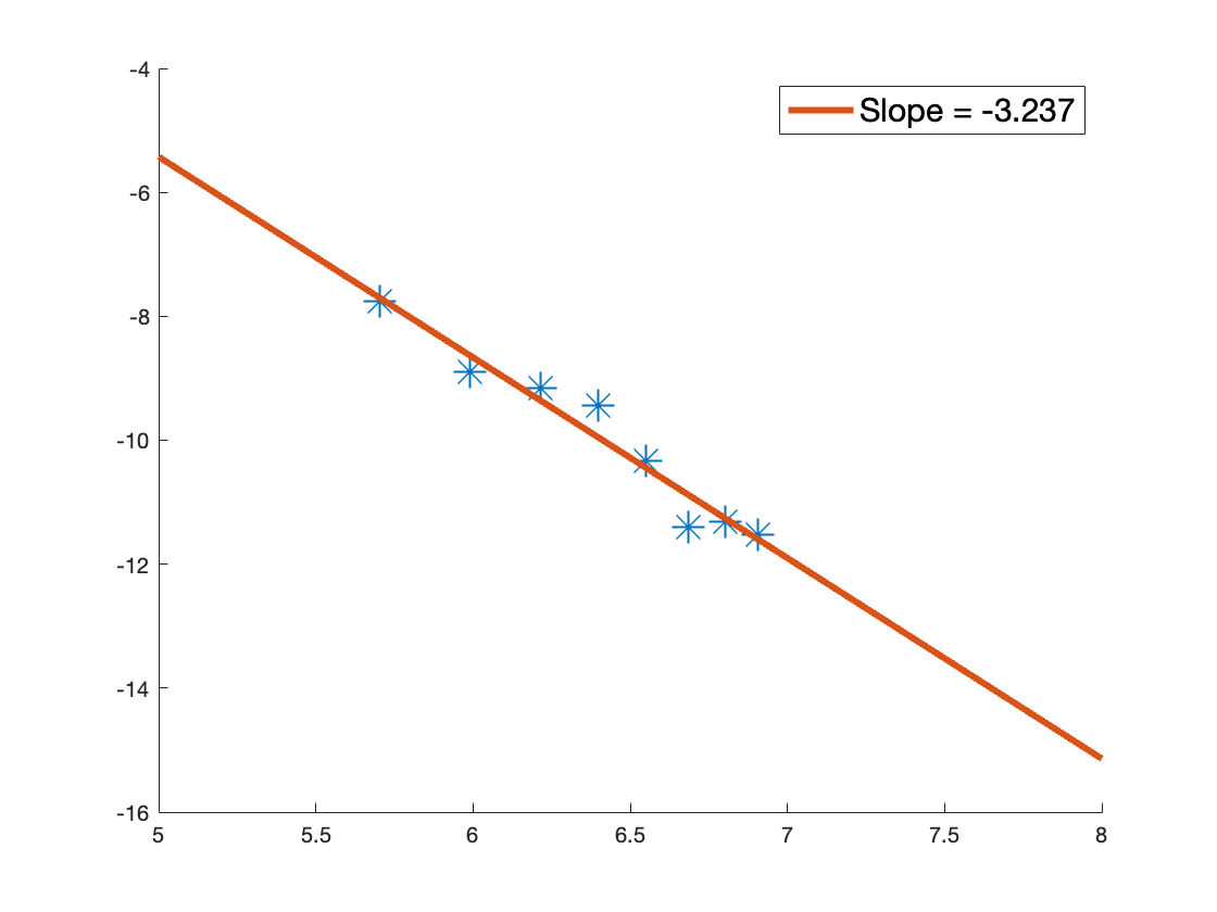
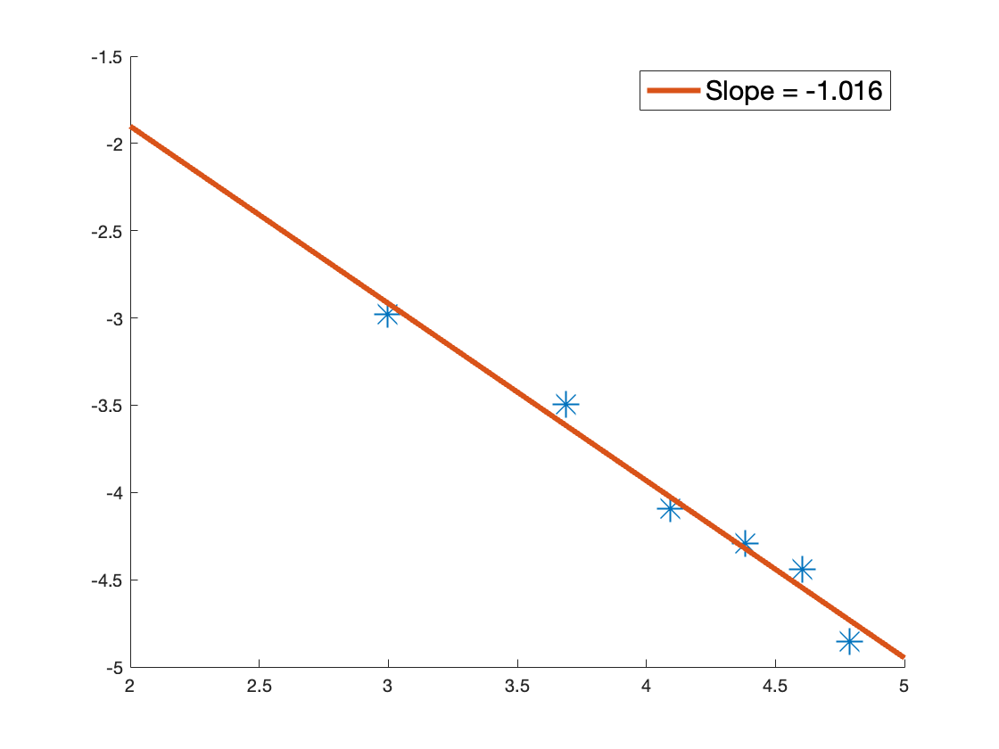
$f=\sin(\pi x)\sin(\pi y)\sin(\pi u)\sin(\pi v)$	$f=\sin(\pi x)\sin(\pi y)\sin(\pi z)\sin(\pi u)\sin(\pi v)\sin(\pi w)$
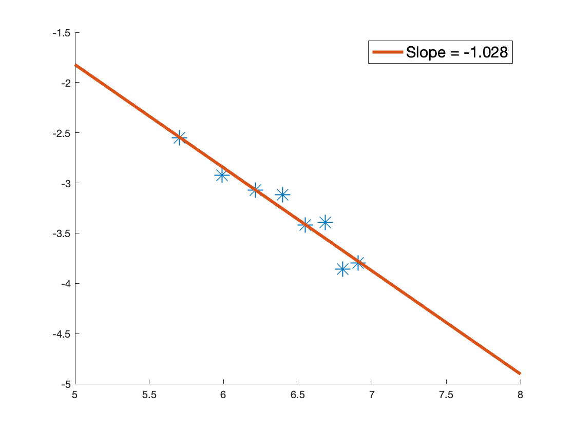
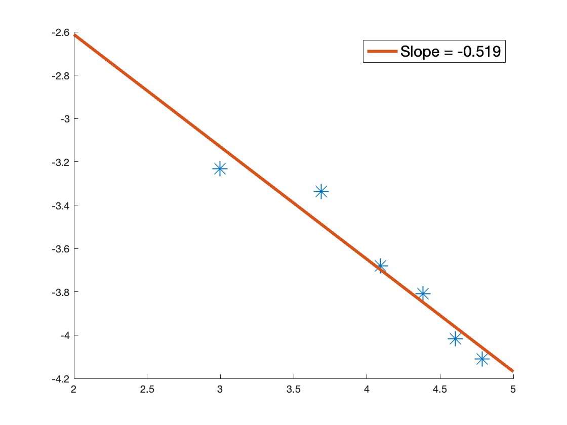
$f=\max(x+y+u+v-2,0)$	$f=\max(x+y+z+u+v+w-3,0)$

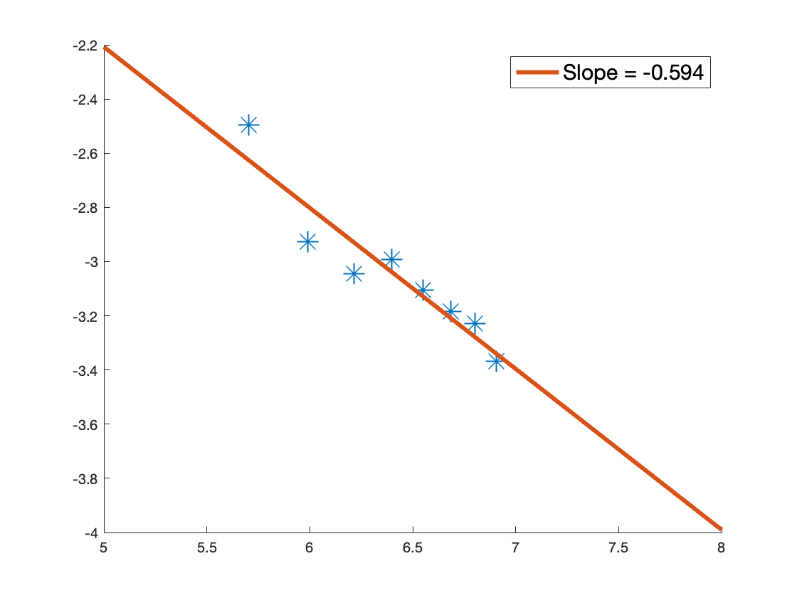
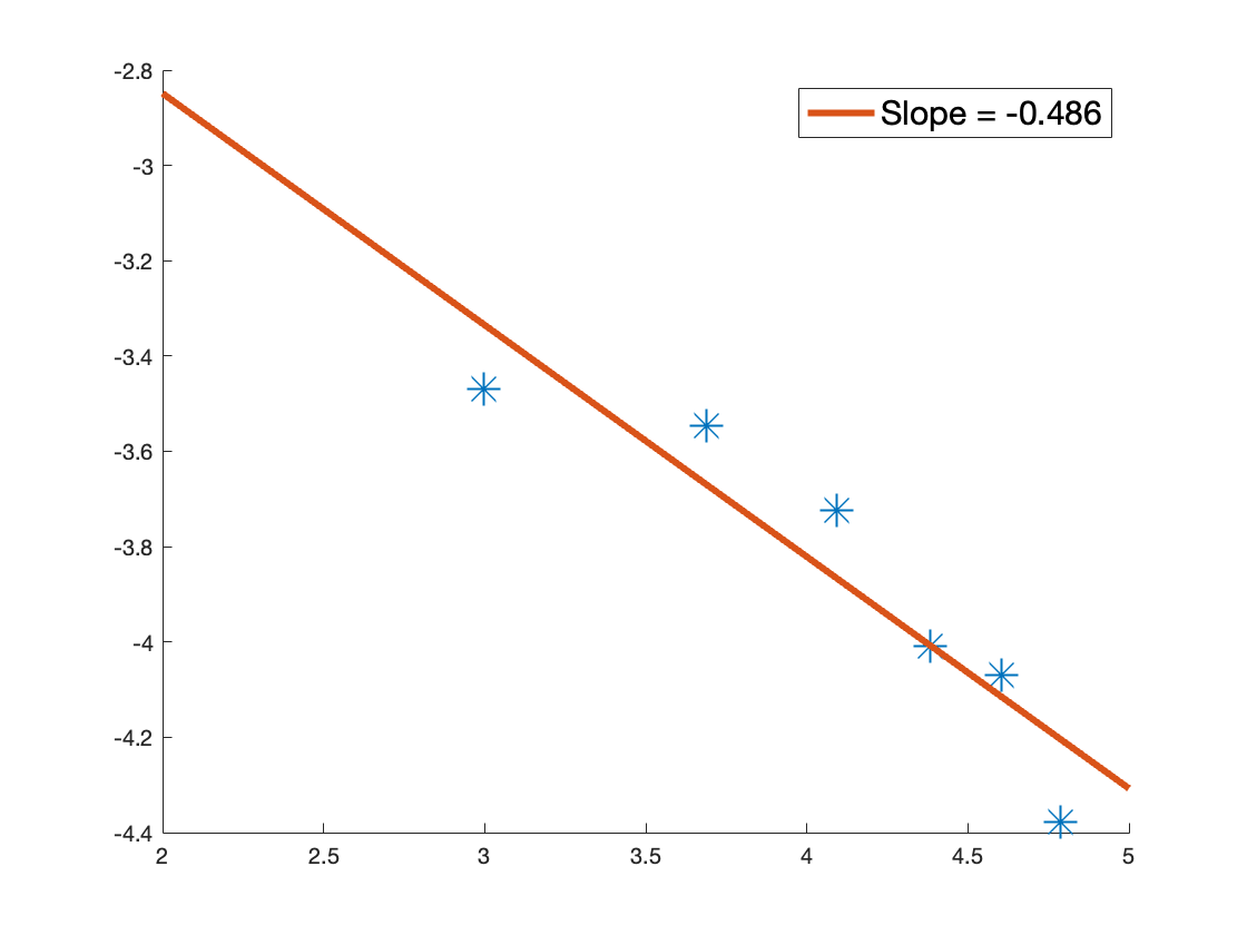
Figure 3: Plots of convergence rate on the Log-log scale in 4D and 6D based on pivotal dataset.

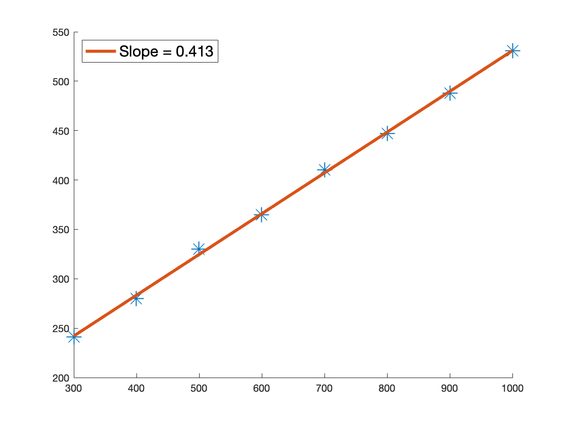
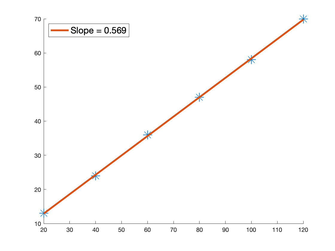
Figure 4: Number of pivotal locations (vertical axis) against $n$ (horizontal axis) in 4D (left) and in 6D (right).

5 Application to Numerically Solving the Poisson Equation

One of the powerful aspects of the LKB-splines based approximation scheme is that we can use it to solve the partial differential equations. To start with, let us consider the Poisson equation:

$$\left\{\begin{array}[]{lll}\Delta u&=&f,{\bf x}\in\Omega\cr u&=&0,{\bf x}\in\partial\Omega.\end{array}\right.$$ (25)

For simplicity, let us consider the 2D case where $\Omega=[0,1]^{2}$. Let us use the $f_{i}=LKB_{i},i=1,\cdots,2n$ as the right-hand side of (25). We can use bivariate spline function of degree $d=8$ and $r=2$ to solve (25) by using the spline collocation method as proposed in [24] to obtain the solution $u_{i}$ $i=1,\cdots,2n$. These form a set of basic Poisson solutions. Then for any $f$, we use $LKB_{i},i=1,\cdots,2n$ to approximate $f$. As discussed in the previous section, we can use a small number of $LKB_{i}$ to approximate $f$ very well. Letting $f=\sum_{i=1}^{2n}c_{i}(f)LKB_{i}$ be a good approximation of $f$, the solution $u$ of the Poisson equation (25) can be well approximated by

$$u_{n}=\sum_{i=1}^{2n}c_{i}(f)u_{i}.$$ (26)

To show $u-u_{n}$ goes to $0$ when $n\to\infty$, we consider $\|\Delta(u-u_{n})\|_{L^{2}(\Omega)}$ which is $\|f-\sum_{i=1}^{n}c_{i}(f)LKB_{i}\|_{L^{2}(\Omega)}$. Let us recall a basic result from [24]. Define a new norm $\|u\|_{L}$ on $H^{2}(\Omega)\cap H^{1}_{0}(\Omega)$ for the Poisson equation as follows.

$$\|u\|_{L}=\|\Delta u\|_{L^{2}(\Omega)}.$$ (27)

Lai and Lee in [24] showed that the new norm is equivalent to the standard norm on Banach space $H^{2}(\Omega)\cap H^{1}_{0}(\Omega)$. That is,

Theorem 6

Suppose $\Omega\subset\mathbb{R}^{d}$ be a bounded domain and the closure of $\Omega$ is of uniformly positive reach $r_{\Omega}>0$. Then there exist two positive constants $A$ and $B$ such that

$$A\|u\|_{H^{2}(\Omega)}\leq\|u\|_{L}\leq B\|u\|_{H^{2}},\quad\forall u\in H^{2}(\Omega)\cap H^{1}_{0}(\Omega),$$ (28)

where $\|\cdot\|_{H^{2}(\Omega)}$ is the standard $H^{2}$ norm for the Sobolev space $H^{2}(\Omega)$.

For convenience, let $\epsilon_{1}=\|f-\sum_{i=1}^{n}c_{i}(f)LKB_{i}\|_{L^{2}(\Omega)}$, where $\Omega=[0,1]^{2}$ which is convex and hence, has an uniformly positive reach. The results in Theorem 6 show that

$$\|u-u_{n}\|_{H^{2}(\Omega)}\leq\epsilon_{1}/A.$$

As in the previous section, $\epsilon_{1}\to 0$ if $f$ is K-Lipschitz continuous, we can further show the following results by using the arguments in [24]:

Theorem 7

Suppose $\Omega\subset\mathbb{R}^{d}$ is a bounded domain and the closure of $\Omega$ is of uniformly positive reach $r_{\Omega}>0$. Suppose that $u\in H^{3}(\Omega)$. Then we have the following inequalities:

$$\|u-u_{n}\|_{L^{2}(\Omega)}\leq C|\triangle|^{2}\epsilon_{1}\hbox{ and }\|\nabla(u-u_{n})\|_{L^{2}(\Omega)}\leq C|\triangle|\epsilon_{1}$$

for a positive constant $C=1/A$, where $A$ is one of the constants in Theorem 6 and $|\triangle|$ is the size of the underlying triangulation $\triangle$.

5.1 Numerical results

For numerical experiments, we will use the following six functions as testing functions for the solution of (25). Their right-hand-side $f$ can be easily computed.

$$u_{1} = x(1-x)y(1-y)/4;$$

$$u_{2} = \sin(\pi x)\sin(\pi y);$$

$$u_{3} = \sin(x)(1-x)(1-y)\sin(y);$$

$$u_{4} = (x(1-x)y(1-y)/4)^{2};$$

$$u_{5} = (\sin(\pi x)\sin(\pi y))^{2};$$

$$u_{6} = (\sin(x)(1-x)(1-y)\sin(y))^{2};$$

We first use the linear LKB-splines to approximate the right-hand-side $f$ associated with $u_{1},\cdots,u_{6}$ over $[0,1]^{2}$. We sampled $101^{2}$ equally-spaced data across $[0,1]^{2}$ and fit the discrete least squares (DLS) approximation of a continuous function $f$ with LKB-splines as basis, and we check the RMSEs based on $1001^{2}$ equally-spaced data across $[0,1]^{2}$. See Table 3 for the numerical results.

Table 3: RMSEs (computed based on $1001^{2}$ equally-spaced locations) of the approximation for the right-hand-side function $f=\Delta u$ based on equally-space sampled data and pivotal locations.

	$n=100$		$n=300$		$n=1000$
# Sampled Data	$101^{2}$	$59$	$101^{2}$	$76$	$101^{2}$	$136$
$\Delta u_{1}$	4.90e-04	9.67e-04	2.46e-04	5.39e-04	1.01e-04	2.91e-04
$\Delta u_{2}$	3.04e-02	4.35e-02	1.31e-02	2.22e-02	3.90e-03	6.98e-03
$\Delta u_{3}$	2.00e-03	3.80e-03	1.00e-03	2.30e-03	3.77e-04	1.10e-03
$\Delta u_{4}$	9.05e-05	1.32e-04	3.85e-05	8.59e-05	6.98e-06	1.86e-05
$\Delta u_{5}$	2.38e-01	4.26e-01	1.13e-01	1.53e-01	2.83e-02	6.06e-02
$\Delta u_{6}$	1.50e-03	2.20e-03	4.90e-04	9.49e-04	1.20e-04	3.17e-04

Next we compute the spline solution of the Poisson equation for each LKB-spline as the right-hand side of the PDE (25) to obtain $u_{i}$’s. As explained above, we use the coefficients of linear LKB-spline approximation of each right-hand-side function $f$ to form the solution of the Poisson equation. We apply the method described in (26) to approximate the solution of the Poisson equation and the numerical results are shown in Table 4. We can see that our method works very well. Similarly, one can use LKB-splines to approximate the solution of the Poisson equation in 3D, we leave the results in [40].

So far we only explained how to use LKB-splines for approximating the solution of the Poisson equation with zero boundary conditions. The underlying domain of interest is $[0,1]^{2}$. This is the most simple PDE. We are currently studying how to use the LKB-splines for the numerical solution of the Poisson equation over arbitrary polygons with nonzero Dirichlet boundary conditions.

Table 4: RMSEs (computed based on $1001^{2}$ equally-spaced locations) of the approximation for the true solution $u$ based on equally-space sampled data and pivotal locations.

	$n=100$		$n=300$		$n=1000$
# Sampled Data	$101^{2}$	$59$	$101^{2}$	$76$	$101^{2}$	$136$
$u_{1}$	1.04e-06	1.57e-05	4.02e-07	5.97e-06	8.09e-08	1.92e-06
$u_{2}$	1.82e-04	1.20e-03	5.09e-05	6.95e-04	9.53e-06	1.05e-04
$u_{3}$	4.56e-06	6.30e-05	1.82e-06	2.38e-05	3.23e-07	6.47e-06
$u_{4}$	2.11e-07	6.91e-07	6.71e-08	1.07e-06	8.34e-09	1.05e-07
$u_{5}$	1.80e-03	8.40e-03	5.98e-04	1.90e-03	1.26e-04	1.01e-03
$u_{6}$	4.30e-06	1.15e-05	9.51e-07	9.51e-06	1.50e-07	1.77e-06

The advantage of this approach is that the basic solutions $u_{i}$’s of the Poisson equation can be solved beforehand and stored and one only needs to approximate the right-hand-side function. Note that the right-hand-side function $f$ can be easily approximated based on the pivotal point locations without using a large amount of the function values if $f$ is K-Hölder continuous. This approach provides an efficient method for solving PDE numerically. When $f$ is K-Lipschitz or K-Hölider continuous, the LKB-splines method will give a very good approximation of the right-hand side and hence, the solution of the Poisson equation as demonstrated in this section.

6 Conclusion and Future Research

In this paper, we proposed a new approach for approximating $f\in C([0,1]^{d})$ based on linear spline approximation of the K-outer function via Kolmogorov superposition theorem with the optimal approximation rate $\mathcal{O}(1/n^{2})$ and approximation constant increasing linearly in $d$. We showed that, based on the linear KB-splines approximation of the K-outer function, such optimal approximation rate is achieved for a dense subclass of functions whose K-outer functions are twice continuously differentiable. We also numerically validated that for $d=4$ and $d=6$, such approximation rate and constant can be achieved via LKB-splines based approximation. Finally, we applied such an approximation scheme in solving the Poisson equation numerically and achieved very accurate approximation results.

Future research can be conducted along these directions. Firstly, it is not easy to fully characterize the original function based on the K-outer function, or vice versa. We want to further investigate in this direction. Secondly, there are high oscillating functions such as trigonometric functions with high frequency, which are not easy to approximate well by LKB-splines. We would like to consider using Fourier basis to build up K-Fourier functions instead. Thirdly, we want to extend this idea and apply it to approximating discontinuous functions. Once it is successful, much of the real applications such as images or signals can be analyzed with this new perspective.

Supplementary Information

We have provided a sample of Matlab code as supplementary material to support our numerical results. Other parts of code are available upon request.

References

- [1] K. Allen, M.-J. Lai, Z. Shen, Maximal Volume Matrix Cross Approximation for Image Compression and Least Squares Solution, https://arxiv.org/abs/2309.17403
- [2] G. Awanou, M. -J. Lai, P. Wenston, The multivariate spline method for scattered data fitting and numerical solutions of partial differential equations, Wavelets and splines: Athens (2005), 24–74.
- [3] A. R. Barron. Universal approximation bounds for superpositions of a sigmoidal function, IEEE Transactions on Information theory, 39(3):930–945, 1993.
- [4] A. R. Barron (1994), Approximation and estimation bounds for artificial neural networks, Mach. Learn. 14, 115–133.
- [5] C. de Boor, Efficient computer manipulation of tensor products, ACM Trans. Math. Software 5 (1979), no. 2, 173–182. 65–04.
- [6] G. Cybenko, Approximation by Superpositions of a Sigmoidal Function, Math. Control Signals Systems (1989) 2:303–314.
- [7] I. Daubechies, R. DeVore, S. Foucart, B. Hanin, and G. Petrova, Nonlinear Approximation and (Deep) ReLU Networks, Constructive Approximation 55, no. 1 (2022): 127-172.
- [8] S. Demko. A Superposition Theorem for Bounded Continuous Functions. Proceed- ings of the American Mathematical Society, 66(1):75–78, 1977.
- [9] R. DeVore, B. Hanin, and G. Petrova, Neural Network Approximation, Acta Numerica 30 (2021): 327-444.
- [10] R. Doss. A superposition theorem for unbounded continuous functions. Transactions of the American Mathematical Society, 233:197–203, 1977.
- [11] D. Fakhoury, E. Fakhoury, H. Speleers, ExSpliNet: An Interpretable and Expressive Spline-Based Neural Network. Neural Networks 152 (2022): 332-346
- [12] Z. Feng. Hilbert’s 13th problem. PhD Dissertation, University of Pittsburgh, 2010.
- [13] Fridman, B. ”Improvement in the smoothness of functions in the Kilmogorov superposition theorem.” Do&l. Akad. Nauk. SSSR 177, no. 5 (1967).
- [14] Girosi, F. and Poggio, T. (1989). Representation properties of networks: Kolmogorov’s theorem is irrelevant. Neural Computation, 1(4), 465-469.
- [15] Guliyev, Namig J., and Vugar E. Ismailov. ”Approximation capability of two hidden layer feedforward neural networks with fixed weights.” Neurocomputing 316 (2018): 262-269.
- [16] R. Hecht-Nielsen. Kolmogorov’s mapping neural network existence theorem. In Proceedings of the international conference on Neural Networks, volume 3, pages 11–14. New York: IEEE Press, 1987.
- [17] Henkin, Gennadi Markovich. ”Linear superpositions of continuously differentiable functions.” In Doklady Akademii Nauk, vol. 157, no. 2, pp. 288-290. Russian Academy of Sciences, 1964.
- [18] B. Igelnik and N. Parikh. Kolmogorov’s spline network. IEEE Transactions on Neural Networks, 14(4):725–733, 2003.
- [19] Klusowski, Jason M., and Andrew R. Barron. ”Approximation by Combinations of ReLU and Squared ReLU Ridge Functions With and Controls.” IEEE Transactions on Information Theory 64, no. 12 (2018): 7649-7656.
- [20] Køurkovà, Vera. ”Kolmogorov’s theorem is relevant.” Neural computation 3, no. 4 (1991): 617-622.
- [21] Køurkovà, Vera. ”Kolmogorov’s theorem and multilayer neural networks.” Neural networks 5, no. 3 (1992): 501-506.
- [22] Kolmogorov, Andrei Nikolaevich. ”On the representation of continuous functions of many variables by superposition of continuous functions of one variable and addition.” In Doklady Akademii Nauk, vol. 114, no. 5, pp. 953-956. Russian Academy of Sciences, 1957.
- [23] M. -J. Lai, Multivariate splines for Data Fitting and Approximation, the conference proceedings of the 12th Approximation Theory, San Antonio, Nashboro Press, (2008) edited by M. Neamtu and Schumaker, L. L. pp. 210–228.
- [24] M.-J. Lai and J. Lee, A multivariate spline based collocation method for numerical solution of partial differential equations, SIAM J. Numerical Analysis, vol. 60 (2022) pp. 2405–2434.
- [25] M. -J. Lai and L. L. Schumaker, Spline Functions over Triangulations, Cambridge University Press, 2007.
- [26] M. -J. Lai and L. L. Schumaker, Domain Decomposition Method for Scattered Data Fitting, SIAM Journal on Numerical Analysis, vol. 47 (2009) pp. 911–928.
- [27] M. -J. Lai and Z. Shen. ”The Kolmogorov Superposition Theorem can Break the Curse of Dimensionality When Approximating High Dimensional Function, submitted, 2023.
- [28] Ji-Nan Lin, and Rolf Unbehauen. ”On the realization of a Kolmogorov network.” Neural Computation 5, no. 1 (1993): 18-20.
- [29] G. G. Lorentz. ”Metric entropy, widths, and superpositions of functions.” The American Mathematical Monthly 69, no. 6 (1962): 469-485.
- [30] G. G. Lorentz, Approximation of Functions, Holt, Rinehart and Winston, Inc. 1966.
- [31] Vitaly Maiorov and Allan Pinkus. ”Lower bounds for approximation by MLP neural networks.” Neurocomputing 25, no. 1-3 (1999): 81-91.
- [32] H. Mhaskar, C. A. Micchelli, Approximation by superposition of sigmoidal and radial basis functions, Adv. Appl. Math. 13 (3) (1992) 350–373.
- [33] Hadrien Montanelli and Haizhao Yang. ”Error bounds for deep ReLU networks using the Kolmogorov–Arnold superposition theorem.” Neural Networks 129 (2020): 1-6.
- [34] Morris, Sidney. ”Hilbert 13: Are there any genuine continuous multivariate real-valued functions?.” Bulletin of the American Mathematical Society 58, no. 1 (2021): 107-118.
- [35] P. A. Ostrand. Dimension of metric spaces and Hilbert’s problem 13. Bulletin of American Mathematical Society, 71(4):619–622, 1965.
- [36] A. Pinkus, Approximation theory of the MLP model in neural networks, Acta Numerica (1999), pp. 143–195.
- [37] M. J. Powell, Approximation theory and methods, Cambridge University Press, 1981.
- [38] Johannes Schmidt-Hieber, ”The Kolmogorov–Arnold representation theorem revisited.” Neural networks 137 (2021): 119-126.
- [39] J. W. Siegel and J. Xu. ”High-order approximation rates for neural networks with ReLUk activation functions. arXiv e-prints.” arXiv preprint arXiv:2012.07205 (2020).
- [40] Z. Shen, Sparse Solution Techniques for Graph Clustering and Function Approximation. Ph.D. Dissertation, University of Georgia, 2024.
- [41] D. A. Sprecher, Ph.D. Dissertation, University of Maryland, 1963
- [42] D. A. Sprecher, ”On the structure of continuous functions of several variables.” Transactions of the American Mathematical Society 115 (1965): 340-355.
- [43] D. A. Sprecher, On the structure of continuous functions of several variables. Transactions of the American Mathematical Society, 115:340–355, 1965.
- [44] D. A. Sprecher, On the structure of representation of continuous functions of several variables as finite sums of continuous functions of one variable. Proceedings of the American Mathematical Society, 17(1):98–105, 1966.
- [45] D. A. Sprecher, An improvement in the superposition theorem of Kolmogorov. Journal of Mathematical Analysis and Applications, 38(1):208–213, 1972.
- [46] Y. Sternfeld, ”Dimension, superposition of functions and separation of points, in compact metric spaces.” Israel Journal of Mathematics 50 (1985): 13-53.
- [47] A. G. Vitushkin, “On the Hilbert’s thirteenth problem”. Soviet Mathematics Doklady, vol. 95 (1954), pp. 701–704.
- [48] A. G. Vitushkin,”A proof of the existence of analytic functions of several variables not representable by linear superpositions of continuously differentiable functions of fewer variables.” In Doklady Akademii Nauk, vol. 156, no. 6, pp. 1258-1261. Russian Academy of Sciences, 1964.