Tiny Time Mixers (TTMs): Fast Pre-trained Models for Enhanced Zero/Few-Shot Forecasting of Multivariate Time Series
Abstract
Large pre-trained models for zero/few-shot learning excel in language and vision domains but encounter challenges in multivariate time series (TS) due to the diverse nature and scarcity of publicly available pre-training data. Consequently, there has been a recent surge in utilizing pre-trained large language models (LLMs) with token adaptations for TS forecasting. These approaches employ cross-domain transfer learning and surprisingly yield impressive results. However, these models are typically very slow and large (billion parameters) and do not consider cross-channel correlations. To address this, we present Tiny Time Mixers (TTM), a significantly small model based on the lightweight TSMixer architecture. TTM marks the first success in developing fast and tiny general pre-trained models (1M parameters), exclusively trained on public TS datasets, with effective transfer learning capabilities for forecasting. To tackle the complexity of pre-training on multiple datasets with varied temporal resolutions, we introduce several novel enhancements such as adaptive patching, dataset augmentation via downsampling, and resolution prefix tuning. Moreover, we employ a multi-level modeling strategy to effectively model channel correlations and infuse exogenous signals during fine-tuning, a crucial capability lacking in existing benchmarks. TTM shows significant accuracy gains (12-38%) over popular benchmarks in few/zero-shot forecasting. It also drastically reduces the compute needs as compared to LLM-TS methods, with a 14X cut in learnable parameters, 106X less total parameters, and substantial reductions in fine-tuning (65X) and inference time (54X). In fact, TTM’s zero-shot often surpasses the few-shot results in many popular benchmarks, highlighting the efficacy of our approach. Code and pre-trained models will be open-sourced.
1 Introduction
Multivariate time series (TS) forecasting entails predicting future values for multiple interrelated time series based on their historical data. This field has advanced significantly, applying statistical and machine learning (ML) methods Hyndman and Athanasopoulos (2021) across domains like weather, traffic, retail, and energy. In general, each time series represents a variable or channel111“Channel” refers to the individual time series in multivariate data (i.e., a multivariate TS is a multi-channel signal).. In certain applications, non-forecasting variables, categorized as controllable and uncontrollable external factors, impact the variables to forecast. We term these non-forecasting variables as exogenous, and the variables requiring forecast as target variables.
Related Work: Recent advances in multivariate forecasting have been marked by the advent of transformer-based Vaswani et al. (2017) approaches, exemplified by models like PatchTST Nie et al. (2023), Autoformer Wu et al. (2021), Informer Zhou et al. (2021), and FEDFormer Zhou et al. (2022). These models have demonstrated notable improvements over traditional statistical and ML methods. Furthermore, architectures based on MLP-Mixer Tolstikhin et al. (2021), such as TSMixer Ekambaram et al. (2023), have emerged as efficient transformer alternatives, boasting 2-3X reduced compute and memory requirements with no accuracy compromise compared to their transformer counterparts. However, none of these advanced approaches have successfully demonstrated the ability to create general pre-trained models that can successfully transfer the learning to unseen target TS dataset, in a similar way as popularly witnessed in NLP and vision tasks. This is very challenging in the TS domain due to the diverse nature of the datasets across applications and the limited public availability of TS data for pre-training. There are existing self-supervised pre-training TS approaches using masked modeling and contrastive learning techniques such as SimMTM Dong et al. (2023) and TF-C Zhang et al. (2022) that offer transfer learning between two datasets when carefully selected based on the dataset properties. However, they fail to provide universal transfer learning capabilities across datasets. Consequently, there has been a recent growing trend to employ pre-trained large language models (LLMs) for TS forecasting, treating it as a cross-domain transfer learning task. These universal cross-transfer approaches, specifically recent works such as LLMTime Gruver et al. (2023) and GPT4TS Zhou et al. (2023) yield promising results in few/zero-shot forecasting approaches. These models are bootstrapped from GPT-2/3 or LLAMA-2 with suitable tokenization strategies to adapt to time-series domains.
However, these LLM based TS approaches do not explicitly handle channel correlations and exogenous support in the context of multivariate forecasting. Moreover, these large models, with billions of parameters, demand significant computational resources and runtime. Hence, in this paper, we focus on building pre-trained models from scratch solely using TS data. Unlike language, which has abundant public pre-training data in terabytes, time-series data is relatively scarce, very diverse and publicly limited. Its scarcity leads to overfitting when pre-training “large” models solely on time-series data. This prompts a question: Can smaller models pre-trained purely on limited public diverse TS datasets give better zero/few-shot forecasting accuracy? Surprisingly, the answer is yes! Toward this, we propose Multi-level Tiny Time Mixers (TTM), a significantly smaller model (1M parameters) based on the lightweight TSMixer architecture, exclusively trained on diverse TS corpora for effective zero/few-shot multivariate TS forecasting via transfer learning.
In particular, TTM is pre-trained using multiple public datasets ( 244M samples) from the Monash data repository222Accessible at https://forecastingdata.org/ Godahewa et al. (2021)). Note that the datasets exhibit considerable diversity in terms of characteristics, such as the different domains, temporal resolution333Resolution refers to the sampling rate of the input time series (e.g., hourly, 10 minutes, 15 minutes, etc.) (spanning from second to daily), lengths, and number of channels. Pre-training on such heterogeneous datasets cannot be handled directly by TSMixer or existing state-of-the-art (SOTA) models. Hence, TTM proposes the following enhancements to the TSMixer architecture: (i) Adaptive Patching across layers, considering the varied suitability of patch lengths for different datasets, (ii) Dataset Augmentation via Downsampling to increase coverage and samples across different resolutions, (iii) Resolution Prefix Tuning to explicitly embed resolution information in the first patch, facilitating resolution-conditioned modeling, particularly beneficial in scenarios with short history lengths. Moreover, our approach leverages multi-level modeling, where TTMs are first pre-trained in a channel-independent way and then seamlessly integrate channel mixing during fine-tuning to model target data-specific channel-correlations and exogenous infusion
Below, we outline the paper’s key contributions:
-
•
Amidst the prevalence of large pre-trained models demanding significant compute and training time (in weeks), our work is the first to showcase the efficacy of building Fast and Tiny Pre-trained models (1M parameters) exclusively trained on Public TS datasets in a flash of just few hours (4-8 hours, 6 A100 GPUs). TTM successfully demonstrates transfer learning to diverse, unseen target datasets for zero/few-shot forecasting, addressing the data scarcity issues prevalent in time series.
-
•
Pre-training on heterogeneous multi-resolution datasets cannot be handled effectively by TSMixer or other SOTA models. Hence, we propose various architectural and training enhancements, such as adaptive patching, data augmentation via downsampling, and (an optional) resolution prefix tuning for robust pre-training.
-
•
TTM employs a multi-level modeling strategy to explicitly model channel-correlations, and incorporates exogenous signals – a crucial capability lacking in LLMs-based TS approaches.
-
•
With extensive evaluation on 11 datasets, TTM shows significant accuracy gains over popular benchmarks (12-38% in few/zero-shot forecasting). It also drastically reduces the compute needs as compared to LLM-TS methods, with a 14X cut in learnable parameters, 106X less total parameters, and substantial reductions in finetuning (65X), inference time (54X), and memory usage (27X).
-
•
The zero-shot results of TTM often surpass the few-shot results of many SOTA approaches, highlighting the effectiveness of our approach.
2 TTM Components
Let be a multivariate time series of length and number of channels. The forecasting task can be formally defined as predicting the future values given the history . Here, denotes the forecast horizon and denotes number of forecast channels, where . The predictions from the model are denoted by . In a general multivariate forecasting task, each channel or variable falls into one of the following categories: (a) Target variables (mandatory):corresponding to the channels for which forecasts are required, (b) Exogenous variables (optional):encompassing (i) uncontrolled variables that may influence the forecasts and assumed to be known or estimated for the forecast period (e.g. weather), and (ii) control variables whose future values during the forecast horizon can be manipulated to govern the behavior of the target variables. (e.g. discount in sales forecasting, operator controls in industrial applications). In TTM, uncontrolled and control variables are treated similarly, as both are considered available during forecasting.
2.1 Multi-level Modeling
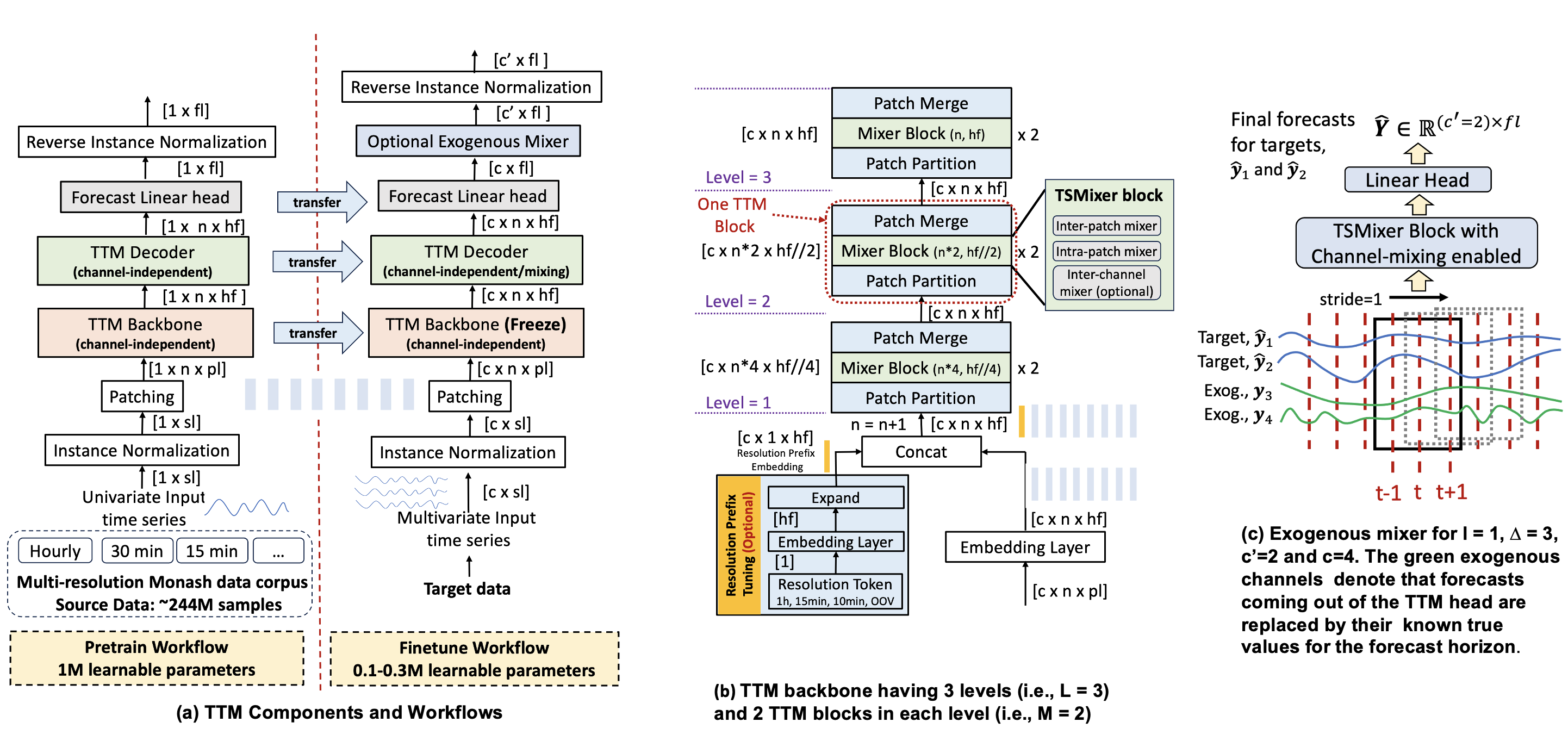
TTM follows a multi-level architecture consisting of four key components (see Figure 1(a)): (1) The TTM Backbone is assembled using building blocks derived from the efficient TSMixer architecture Ekambaram et al. (2023). TSMixer is based on simple MLP blocks that enable mixing of features within patches, across patches and channels, surpassing existing transformer-based TS approaches with minimal computational requirements. Since TSMixer is not targeted to handle multi-resolution data, we introduce various novel enhancements to it as explained later. (2) TTM Decoderfollows the same backbone architecture but is considerably smaller in size, approximately 10-20% of the size of the backbone, (3) Forecast Headconsists of a linear head designed to produce the forecast output, and (4) Optional Exogenous Mixer serves to fuse exogenous data into the model’s forecasting process. This multi-level model refactoring is required to dynamically change the working behavior of various components based on the workflow type, as explained in Section 3. In addition to the above primary components, we also have a preprocessing component as explained next.
2.2 Pre-processing
As shown in Figure 1(a) with colorless blocks, the historical time series is first normalized per instance to have zero mean and unit standard deviation for each channel dimension, to tackle any possible distribution shifts Nie et al. (2023); Ekambaram et al. (2023). This process is reversed at the end before computing the loss. The normalized data is subsequently patched into non-overlapping windows, each of length and then, passed to the TTM backbone. Patching, as introduced in Nie et al. (2023), has proven to be highly valuable for forecasting. Its effectiveness lies in preserving local semantic information, accommodating longer history, and reducing computation.
3 TTM Workflows
TTM works in 2 stages: pre-train and fine-tune (Figure 1(a)).
3.1 Pre-training Workflow
In the pre-training stage, we train the model on a large collection of public datasets from the Monash data repositoryGodahewa et al. (2021). Since the primary focus of TTM is forecasting, pre-training is modeled with a direct forecasting objective. TTM is first pre-trained in a univariate fashion with independent channels on all the existing datasets. Due to varied channel counts in pre-training datasets, modeling multivariate correlations is not feasible here; it is addressed later during fine-tuning. Multivariate pre-training datasets are initially transformed into independent univariate time series . These are pre-processed (Section 2.2), and subsequently fed into the TTM backbone for multi-resolution pre-training. The output of the backbone is passed through the decoder and forecast head to produce the forecast which is then reverse-normalized to bring back to the original scale. We pre-train the TTM with mean squared error (MSE) loss function calculated over the forecast horizon: . Thus for a given input context length and forecast length , we get a pre-trained model capturing the common temporal forecasting dynamics and seasonal patterns as observed in the overall pre-training data.
3.1.1 Multi-Resolution Pre-training via TTM Backbone
The majority of the pre-training happens in the TTM backbone. The primary challenge with the proposed pre-training technique is that the pre-training data is diverse and has multiple resolutions. There are two main options for pre-training: conducting separate pre-training for each resolution type or pre-training using all resolution data collectively. While it’s common to train a model per resolution type to overcome challenges in learning diverse seasonal patterns, this leads to diminished training data for each resolution due to limited data availability. Consequently, this motivated the exploration of pre-training a single model using datasets from all resolutions. To achieve this, we propose the following 3 enhancements.
Adaptive Patching: The TTM backbone is crafted with an adaptive patching architecture where different layers of the backbone operate at varying patch lengths and numbers of patches. Since each dataset in the pre-training corpora may perform optimally at a specific patch length, this approach greatly aids in generalization when diverse datasets with different resolutions are introduced. As shown in Figure 1(b), the patched data is passed through a embedding layer to project it to the patch hidden dimension, . Optionally, if the resolution prefix tuning module is activated (as explained later), the resolution prefix is concatenated with . For notational simplicity, we denote the concatenated tensor with as well.
The TTM backbone consists of levels, each comprising TTM blocks with identical patch configurations. A TTM block in the -th level, , receives the processed data from the earlier block. Each TTM block is further comprised of a patch partition model, a vanilla TSMixer block, and a patch merging block. Patch Partition block at every level increases the number of patches by a factor of and reduces the patch dimension size by the same factor by reshaping , where . Note that, we set for some integer . Then, TSMixer is applied to the adapted data . Finally, the output from TSMixer is again reshaped to its original shape (i.e., ) in the patch merging block. Note that, as we go deeper into the network, the number of patches decreases while the patch dimension size increases leading to adaptive patching which helps in better generalization as we pre-train with multiple datasets together. This idea of adaptive patching is popular and very successful in the vision domain (E.g. Swin transformers Liu et al. (2021) and we are the first to port it successfully to the time-series domain to resolve multi-resolution issues in pre-training with diverse TS datasets. Figure 1(b) shows the TTM backbone for and . Please note that adaptive patching is enabled only in the backbone and not in the decoder, which is designed to be very lightweight.
Data Augmentation via Downsampling: A significant challenge in TS pre-training datasets is the scarcity of public datasets at specific resolutions. To overcome this, we employ a downsampling technique for high-resolution datasets, generating multiple datasets at lower resolutions. For example, from a one-second resolution dataset, we derive datasets at minute and hour resolutions. Note that, the original high-resolution dataset remains within the pool of pre-training datasets. This methodology significantly augments the number of datasets for each resolution which greatly improves the model performance (Section 4.5).
Resolution Prefix Tuning: This technique explicitly learns and incorporates a new patch embedding as a prefix into the input data based on the input resolution type (see Figure 1(b)). Similar to the concept of prefix tuning Li and Liang (2021), this approach provides an explicit signal to the model about the resolution type for resolution-conditioned modeling. First, we map every resolution to a unique integer, which is then passed through an embedding layer to project it to the hidden dimension, . Subsequently, we expand the embedding across all channels to have a representation of shape . This module is optional for the TTM backbone, particularly beneficial when the context length () is short. In these scenarios, automatically detecting the resolution becomes a challenge for the model. Hence, by explicitly fusing the resolution information as a prefix, we can enhance the model’s ability to learn effectively across resolutions.
3.2 Fine-tuning Workflow
In the fine-tuning workflow, we deal with data from the target domain that has no overlap with the pre-training datasets. We have three options here: (a) In Zero-shot forecasting, we directly use the pre-trained model to evaluate on the test part of the target data, (b) In Few-shot forecasting, we utilize only a tiny portion (5-10%) of the train part of the target data to quickly update the pre-trained weights of the decoder and head, and subsequently, evaluate it on the test part, (c) In Full-shot forecasting, we fine-tune the pre-trained weights of the decoder and head on the entire train part of the target data, and then, evaluate on the test part.
The backbone is completely frozen during fine-tuning, and still operates in a channel-independent univariate fashion. However, the TTM decoder can be fine-tuned via channel-mixing (for multivariate) or a channel-independent (for univariate) way based on the nature of the target data. If pure multivariate modeling is needed, then the channel-mixer block in all the TSMixer components (see Figure 1(b)) in the decoder gets enabled to explicitly capture the channel correlation between the channels. The forecast head and reverse normalization perform similar operations as in the pre-training stage. The fine-tuning also optimizes the forecasting objective with MSE loss. This thoughtful multi-level design choice ensures our backbone excels in channel-independent pre-training, enabling effective temporal correlation modeling across diverse datasets. Simultaneously, the decoder handles target-data-specific tasks like channel-correlation modeling and fine-tuning. In addition, if the target data has exogenous variables, then an exogenous mixer block is applied to the actual forecasts as explained next.
Exogenous Mixer Block: As described in Section 2, the future values of the exogenous channels are known in advance. Let the forecast from the forecast head be . Let the channels denote the target variables and denote all exogenous variables with their future values known. First, we replace the forecast values for the exogenous channels with the true future values () and transpose it: . Next, to learn inter-channel lagged correlations, we patch into a series of overlapped windows (i.e., patching with stride) to create a new tensor: , where with being the context length to incorporate on either side of a time point444This needs padding with zeros of length on both sides.. Subsequently, we pass through a vanilla TSMixer block with channel mixing enabled. Thus, the lagged dependency of the forecasts for the target channels on the exogenous channels is seamlessly learned. Finally, we attach a linear head to produce the forecasts for the target channels which is then reshaped as . Figure 1(c) depicts this procedure.
| Zero-shot | Few-shot (5%) | |||||||||
| TTM | TTM | GPT4TS | PatchTST | TSMixer | TimesNet | Dlinear | FEDFormer | Autoformer | ||
| ETTH1 | 96 | 0.365 | 0.366 | 0.543 | 0.557 | 0.554 | 0.892 | 0.547 | 0.593 | 0.681 |
| 192 | 0.393 | 0.391 | 0.748 | 0.711 | 0.673 | 0.940 | 0.720 | 0.652 | 0.725 | |
| 336 | 0.415 | 0.421 | 0.754 | 0.816 | 0.678 | 0.945 | 0.984 | 0.731 | 0.761 | |
| 720 | 0.538 | - | - | - | - | - | - | - | - | |
| ETTH2 | 96 | 0.285 | 0.282 | 0.376 | 0.401 | 0.348 | 0.409 | 0.442 | 0.390 | 0.428 |
| 192 | 0.341 | 0.338 | 0.418 | 0.452 | 0.419 | 0.483 | 0.617 | 0.457 | 0.496 | |
| 336 | 0.383 | 0.383 | 0.408 | 0.464 | 0.389 | 0.499 | 1.424 | 0.477 | 0.486 | |
| 720 | 0.441 | - | - | - | - | - | - | - | - | |
| ETTM1 | 96 | 0.413 | 0.359 | 0.386 | 0.399 | 0.361 | 0.606 | 0.332 | 0.628 | 0.726 |
| 192 | 0.476 | 0.402 | 0.440 | 0.441 | 0.411 | 0.681 | 0.358 | 0.666 | 0.750 | |
| 336 | 0.553 | 0.424 | 0.485 | 0.499 | 0.467 | 0.786 | 0.402 | 0.807 | 0.851 | |
| 720 | 0.737 | 0.575 | 0.577 | 0.767 | 0.677 | 0.796 | 0.511 | 0.822 | 0.857 | |
| ETTM2 | 96 | 0.187 | 0.174 | 0.199 | 0.206 | 0.200 | 0.220 | 0.236 | 0.229 | 0.232 |
| 192 | 0.261 | 0.240 | 0.256 | 0.264 | 0.265 | 0.311 | 0.306 | 0.394 | 0.291 | |
| 336 | 0.323 | 0.299 | 0.318 | 0.334 | 0.314 | 0.338 | 0.380 | 0.378 | 0.478 | |
| 720 | 0.436 | 0.407 | 0.46 | 0.454 | 0.410 | 0.509 | 0.674 | 0.523 | 0.553 | |
| Weather | 96 | 0.154 | 0.152 | 0.175 | 0.171 | 0.188 | 0.207 | 0.184 | 0.229 | 0.227 |
| 192 | 0.203 | 0.198 | 0.227 | 0.230 | 0.234 | 0.272 | 0.228 | 0.265 | 0.278 | |
| 336 | 0.256 | 0.250 | 0.286 | 0.294 | 0.287 | 0.313 | 0.279 | 0.353 | 0.351 | |
| 720 | 0.329 | 0.326 | 0.366 | 0.384 | 0.365 | 0.400 | 0.364 | 0.391 | 0.387 | |
| Electricity | 96 | 0.169 | 0.142 | 0.143 | 0.145 | 0.147 | 0.315 | 0.150 | 0.235 | 0.297 |
| 192 | 0.196 | 0.162 | 0.159 | 0.163 | 0.172 | 0.318 | 0.163 | 0.247 | 0.308 | |
| 336 | 0.209 | 0.184 | 0.179 | 0.175 | 0.190 | 0.340 | 0.175 | 0.267 | 0.354 | |
| 720 | 0.264 | 0.228 | 0.233 | 0.219 | 0.280 | 0.635 | 0.219 | 0.318 | 0.426 | |
| Traffic | 96 | 0.518 | 0.401 | 0.419 | 0.404 | 0.408 | 0.854 | 0.427 | 0.670 | 0.795 |
| 192 | 0.548 | 0.425 | 0.434 | 0.412 | 0.421 | 0.894 | 0.447 | 0.653 | 0.837 | |
| 336 | 0.55 | 0.437 | 0.449 | 0.439 | 0.477 | 0.853 | 0.478 | 0.707 | 0.867 | |
| 720 | 0.605 | - | - | - | - | - | - | - | - | |
| TTM Zero-shot % IMP | 1% | 3% | 2% | 31% | 6% | 25% | 32% | |||
| TTM 5% Few-shot % IMP | 12% | 14% | 12% | 38% | 17% | 32% | 38% | |||
| Metric | Data | GPT4TS | TTM (Ours) | IMP (X) |
| FT NPARAMS (M) | Weather | 3.2 | 0.29 | (14X) |
| Electricity | 3.2 | 0.29 | ||
| Traffic | 5.5 | 0.29 | ||
| TL NPARAMS (M) | Weather | 84.3 | 0.8 | (106X) |
| Electricity | 84.3 | 0.8 | ||
| Traffic | 86.6 | 0.8 | ||
| EPOCH TIME (s) | Weather | 37 | 1 | (65X) |
| Electricity | 241 | 4 | ||
| Traffic | 782 | 8 | ||
| MAX MEMORY (GB) | Weather | 21.9 | 1.06 | (27X) |
| Electricity | 39.7 | 2.02 | ||
| Traffic | 53.7 | 1.34 | ||
| TEST TIME (s) | Weather | 52.53 | 1.66 | (54X) |
| Electricity | 353.4 | 8.07 | ||
| Traffic | 1163.9 | 13.5 |
| 10% | 25% | 50% | 75% | 100% | IMP | |
| TTM | 0.422 | 0.421 | 0.413 | 0.402 | 0.398 | - |
| SimMTM | 0.591 | 0.535 | 0.491 | 0.466 | 0.415 | 17% |
| Ti-MAE | 0.660 | 0.594 | 0.55 | 0.475 | 0.466 | 24% |
| TST | 0.783 | 0.641 | 0.525 | 0.516 | 0.469 | 28% |
| LaST | 0.645 | 0.610 | 0.540 | 0.479 | 0.443 | 23% |
| TF-C | 0.799 | 0.736 | 0.731 | 0.697 | 0.635 | 43% |
| CoST | 0.784 | 0.624 | 0.540 | 0.494 | 0.428 | 26% |
| TS2Vec | 0.655 | 0.632 | 0.599 | 0.577 | 0.517 | 31% |
4 Experiments and Results
4.1 Experimental Setting
Datasets: Pre-training employs a subset of the Monash data hub Godahewa et al. (2021) of size M samples. We specifically exclude datasets (like yearly, monthly) as they do not possess sufficient length for the long-term forecasting task. Moreover, we remove all the datasets that we utilize for evaluation (i.e., weather, electricity, and traffic). For zero/few-shot evaluation we consider seven public datasets (D1): ETTH1, ETTH2, ETTM1, ETTM2, Weather, Electricity & Traffic as popularly used in most prior SOTA works Zhou et al. (2021); Nie et al. (2023). Since these datasets do not contain any exogenous variables nor exhibit cross-channel correlation benefits, we incorporate four other datasets (D2) for separately validating the efficacy of the decoder channel mixing and exogenous mixer module: bike sharing (BS) Fanaee-T (2013), carbon capture plant (CC) Jablonka et al. (2023), and 2 more datasets from Biz-IT observability domain ITB (2023): Application (APP) and Service (SER). Refer Appendix for full data details.
SOTA Bechmarks: We benchmark TTM with the latest public SOTA forecasting models categorized as follows: (a) LLM-based TS pre-trained models:GPT4TS Zhou et al. (2023), LLMTime Gruver et al. (2023) (b) Self-supervised pre-trained models: SimMTM Dong et al. (2023),Ti-MAE Li et al. (2023), TST Zerveas et al. (2021), LaST Wang et al. (2022), TF-C Zhang et al. (2022), CoST Woo et al. (2022) and Ts2Vec Yue et al. (2022) (c) TS transformer models:PatchTST Nie et al. (2023), FEDFormer Zhou et al. (2022), Autoformer Wu et al. (2021) (d) Other SOTA models:TSMixer Ekambaram et al. (2023), DLinear Zeng et al. (2022) and TimesNet Wu et al. (2022)
| Zero-shot | Few-shot (10%) | ||||||||
| Data | TTM (Ours) | TTM (Ours) | GPT4TS | PatchTST | TSMixer | TimesNet | Dlinear | FEDFormer | Autoformer |
| ETTH1 | 0.428 | 0.422 | 0.590 | 0.633 | 0.578 | 0.869 | 0.691 | 0.639 | 0.702 |
| ETTH2 | 0.362 | 0.360 | 0.397 | 0.415 | 0.370 | 0.479 | 0.605 | 0.466 | 0.488 |
| ETTM1 | 0.545 | 0.458 | 0.464 | 0.501 | 0.441 | 0.677 | 0.411 | 0.722 | 0.802 |
| ETTM2 | 0.302 | 0.278 | 0.293 | 0.296 | 0.282 | 0.320 | 0.316 | 0.463 | 1.342 |
| Electricity | 0.210 | 0.180 | 0.176 | 0.176 | 0.180 | 0.323 | 0.180 | 0.346 | 0.431 |
| Traffic | 0.555 | 0.428 | 0.440 | 0.430 | 0.429 | 0.951 | 0.446 | 0.663 | 0.749 |
| Weather | 0.236 | 0.227 | 0.238 | 0.242 | 0.236 | 0.279 | 0.241 | 0.284 | 0.300 |
| TTM Zero-shot improvements | -4% | -2% | -7% | 27% | 2% | 27% | 39% | ||
| TTM Few-shot (10%) improvements | 7% | 9% | 4% | 34% | 13% | 34% | 45% | ||
| Data | Zero-shot | ||
| LLMTime | TTM | ||
| Traffic | 96 | 0.340 | 0.195 |
| 192 | 0.526 | 0.367 | |
| Weather | 96 | 0.107 | 0.031 |
| 192 | 0.062 | 0.067 | |
| Electricity | 96 | 0.609 | 0.238 |
| 192 | 0.960 | 0.488 | |
| ETTM2 | 96 | 0.167 | 0.164 |
| 192 | 0.198 | 0.228 | |
| TTM IMP (%) | 29% | ||
MSE Improvement (IMP)
in zero-shot setting.
TTM Model Details: For our experiments, we build 5 pre-trained models for the following , configuration: (512,96), (512,192), (512, 336), (512,720) and (96,24). Based on the and requirement of the target dataset, a suitable pre-trained model is selected to initialize the weights accordingly for fine-tuning. Since our pre-trained models are very small, they can be trained quickly in a few hours (4-8 hrs), as opposed to several days/weeks in standard approaches. Hence, pre-training multiple TTM models is no longer a practical constraint. Pre-training is performed in a distributed fashion with 50 CPUs and 6 A100 GPUs with 40 GB GPU memory while fine-tuning uses only 1 GPU. Other model configurations are as follows: patch length = 64 (for 512) and 8 (for 96), stride = , number of levels = 6, number of TTM blocks per level = 2, number of decoder layers = 2, batch size = 3K, number of epochs = 20, and dropout = 0.2. TSMixer specific hyperparameters include feature scaler = 3, hidden feature size = , expansion feature size . Resolution prefix tuning is disabled by default and enabled only for shorter context lengths (as explained in Table. 9). Decoder channel-mixing and exogenous mixer blocks are disabled during pre-training and enabled for D2 datasets during fine-tuning. All other model parameters remain the same across pre-training and fine-tuning except for a few parameters like dropout and batch size that can be adjusted based on the target data. Hyperparameters are selected based on the validation performance, and the test results are reported. For full implementation details, refer to the Appendix. MSE is used as the default evaluation metric.
| BS | CC | APP | SER | % IMP | |
| TTM-CM | 0.582 | 0.250 | 0.042 | 0.114 | |
| TTM-Zero-shot | 0.992 | 0.263 | 0.183 | 0.238 | 44% |
| TTM | 0.635 | 0.261 | 0.073 | 0.143 | 18% |
| PatchTST | 0.735 | 0.267 | 0.060 | 0.119 | 15% |
| TSMixer-CC | 0.651 | 0.284 | 0.053 | 0.136 | 15% |
| TSMixer-CM | 0.716 | 0.303 | 0.069 | 0.118 | 20% |
| TSMixer | 0.664 | 0.267 | 0.066 | 0.134 | 17% |
| GPT4TS | 0.645 | 0.254 | 0.075 | 0.135 | 18% |
4.2 TTM’s Zero/Few-shot Performance
Table 1 compares the performance of TTM model in zero-shot and few-shot (5%) settings across multiple s. Baseline results are reported from Zhou et al. (2023) as we use the same few-shot data filtering strategy as followed in that paper. Note that for zero-shot performance, the pre-trained TTM model is directly evaluated on the test set. The 5% few-shot TTM outperforms the SOTAs in most of the cases with significant accuracy gains (12-38%). An even more impressive observation is that the TTM in zero-shot setting is also able to outperform most of the SOTAs which are trained on 5% of the target data. This observation establishes the generalization ability of the pre-trained TTM model on the target datasets. Likewise, Table 3 shows the 10% few-shot performance of the TTM, where we outperform all the existing SOTAs by 4-45% accuracy gains. In addition, TTM zero-shot also beats many SOTAs (not all) with 10% training highlighting the effectiveness of our approach.
Additionally, we conduct a comparison between TTM and the LLMTime model which is explicitly designed for zero-shot setting. Since these models are based on LLaMA and are massive in size, the authors used only the last window of the standard test-set for faster evaluation, as opposed to using all the windows in the full test-set . Hence, we compare them separately in Table 4 based on the same datasets, , and test-set as reported in Gruver et al. (2023). In this evaluation, we outperform LLMTime by a substantial margin of 29%. In addition, there are alternative pre-training approaches like masked modeling and contrastive learning techniques that may not offer universal transfer learning capabilities across all datasets (like TTM), but they excel in enabling cross-transfer learning between two datasets when carefully selected. Table 2 illustrates the cross-transfer learning from ETTH2 to ETTH1 for these models in various few-shot settings (as reported in Dong et al. (2023)). Notably, TTM, with no specific cross-data selection, outperforms all popular SOTAs, including the latest SimMTM, by 17-43%. Thus, TTM significantly beats all the existing SOTAs including the recent popular transfer learning benchmarks based on LLMs. Notably, we achieve these accuracy gains with significantly reduced compute requirements, as elaborated next.
| Data | Zero-shot | Few-shot (5%)) | Few-shot (10%)) | |||||||
| 5 Epochs | 50 Epochs | 5 Epochs | 50 Epochs | |||||||
| RI | PT | RI | PT | RI | PT | RI | PT | RI | PT | |
| ETTH1 | 0.735 | 0.428 | 0.687 | 0.389 | 0.629 | 0.393 | 0.64 | 0.419 | 0.552 | 0.422 |
| ETTH2 | 0.400 | 0.362 | 0.378 | 0.334 | 0.379 | 0.334 | 0.371 | 0.357 | 0.370 | 0.360 |
| ETTM1 | 0.722 | 0.545 | 0.474 | 0.483 | 0.448 | 0.440 | 0.421 | 0.458 | 0.403 | 0.458 |
| ETTM2 | 0.353 | 0.302 | 0.296 | 0.274 | 0.290 | 0.280 | 0.279 | 0.271 | 0.274 | 0.278 |
| Electricity | 0.890 | 0.210 | 0.356 | 0.188 | 0.199 | 0.179 | 0.220 | 0.186 | 0.178 | 0.180 |
| Traffic | 1.453 | 0.555 | 0.593 | 0.454 | 0.441 | 0.421 | 0.486 | 0.446 | 0.430 | 0.428 |
| Weather | 0.321 | 0.236 | 0.267 | 0.233 | 0.264 | 0.231 | 0.240 | 0.229 | 0.238 | 0.227 |
| IMP | 36% | 21% | 12% | 9% | 2% | |||||
| Data | Zero-shot | Few-shot (10%) | ||
| Vanilla | Adaptive Patching | Vanilla | Adaptive Patching | |
| ETTH1 | 0.501 | 0.428 | 0.478 | 0.422 |
| ETTH2 | 0.375 | 0.362 | 0.372 | 0.360 |
| ETTM1 | 0.577 | 0.545 | 0.463 | 0.458 |
| ETTM2 | 0.310 | 0.302 | 0.272 | 0.278 |
| Electricity | 0.215 | 0.210 | 0.178 | 0.180 |
| Traffic | 0.556 | 0.555 | 0.431 | 0.428 |
| Weather | 0.239 | 0.236 | 0.230 | 0.227 |
| IMP (%) | 4% | 2% | ||
| Data | Zero-shot | |
| Original Data | With Downsample | |
| ETTH1 | 0.603 | 0.379 |
| ETTH2 | 0.351 | 0.313 |
| ETTM1 | 0.852 | 0.444 |
| ETTM2 | 0.261 | 0.224 |
| Electricity | 0.424 | 0.182 |
| Traffic | 0.898 | 0.533 |
| Weather | 0.186 | 0.178 |
| IMP (%) | 30% | |
| Data | = 96 | = 512 | ||
| NP | P | NP | P | |
| ETTH1 | 0.373 | 0.358 | 0.365 | 0.360 |
| ETTH2 | 0.180 | 0.179 | 0.285 | 0.280 |
| ETTM1 | 0.559 | 0.387 | 0.413 | 0.384 |
| ETTM2 | 0.127 | 0.108 | 0.187 | 0.194 |
| Weather | 0.103 | 0.103 | 0.154 | 0.160 |
| Electricity | 0.208 | 0.201 | 0.169 | 0.175 |
| Traffic | 0.754 | 0.740 | 0.518 | 0.518 |
| IMP (%) | 8% | 0% | ||
4.3 Computational Benefits of TTM
Table 2 compares the computational benefits of TTM over GPT4TS, the most popular LLM-TS model and the current best SOTA in few-shot setting. For a fair comparison, we run both models with the best-reported parameters in a single A100 GPU with the same setup (Details in Appendix). Since GPT4TS is based on GPT-2, it consumes a huge model footprint and exhibits slow execution. In specific, TTM achieves 14X cut in Fine-tune (FT) parameters (NPARAMS) and a remarkable 106X reduction in Total (TL) parameters. This reduction in model footprint further leads to a significant reduction in fine-tuning EPOCH TIME by 65X, MAX MEMORY usage by 27X, and total inference time on the entire test data (TEST TIME) by 54X. The computational benefits also apply over other LLM-based time series models like LLMTime, built on LLaMA, which is larger than GPT-2. In fact, LLMTime used a very small test set on these datasets as opposed to the standard test set to overcome this slow-execution.
4.4 TTM’s effectiveness in cross-channel and exogenous modeling
Since the datasets () used in previous experiments do not have exogenous variables, we evaluate the effectiveness of TTM on 4 other datasets (, as explained in 4.1) to quantify its benefits. Since these datasets are already very small, we used their full data for fine-tuning. Table 5 shows the performance of the pre-trained TTM model fine-tuned on the target data with exogenous mixer module and decoder channel-mixing enabled (TTM-CM). We compare the performance of TTM-CM with the pre-trained TTM used in zero-shot setting (TTM-Zero-shot), and plain TTM (TTM) and other primary SOTAs (PatchTST, TSMixer variants, and GPT4TS) trained from scratch. Other SOTAs are not reported here, considering their inferior performance and space constraints. Specifically, we compare with TSMixer with channel-mixing enabled (TSMixer-CM) and TSMixer with Cross-Channel reconciliation head (TSMixer-CC) Ekambaram et al. (2023) as they are the latest SOTAs in channel-correlation modeling. We can see that TTM-CM outperforms all the competitive models with a significant margin (15-44%), thus, demonstrating the power of TTM in capturing inter-channel correlations.
4.5 Ablation Studies
Effect of Pre-training: Table 6 illustrates the advantages of the proposed pre-training (PT) approach in comparison to randomly initialized (RI) model weights. In the case of zero-shot, the pre-trained TTM (PT) exhibits 36% improvement over RI. This outcome is expected, as random weights are directly employed for forecasting with RI. For the 5% few-shot scenario, PT achieves noteworthy improvements of 21% and 12% over RI when fine-tuned for 5 and 50 epochs, respectively. This underscores the utility of pre-trained weights in facilitating quick learning with a limited amount of target data. Even in the case of 10% few-shot, PT continues to demonstrate an improved performance of 9% for 5 epochs and 2% for 50 epochs. Thus, the performance impact of leveraging pre-trained weights greatly increases as the size of the training data and the available time-to-fine-tune reduces.
Effect of Adaptive Patching: The Adaptive patching presented in Section 3.1.1 is a key component of the TTM backbone. Table 7 demonstrates the relative improvements when we employ adaptive patching with respect to a vanilla TTM backbone without this module. We can see that adaptive patching adds an extra 4% improvement during zero-shot and 2% improvement for 10% few-shot. Performance improvements are observed in almost all datasets which justifies the effectiveness of the adaptive patching module when evaluated on multiple datasets of different resolutions.
Effect of Augmentation via Downsampling: Table 8 compares the zero-shot test performances between the TTM model trained on the original Monash data and the TTM trained on the augmented Monash data after downsampling as described in Section 3.1. There is a significant improvement of 30% for the model pre-trained on the augmented datasets as it adds more data coverage across various resolutions. This observation highlights the strength of the proposed TTM model to learn from diverse datasets together, and increasing the number of datasets for each resolution helps.
Effect of Resolution Prefix Tuning: Since resolution prefix tuning explicitly adds the resolution type as an extra embedding, it greatly helps when the input context length is short where it is challenging for the model to derive the resolution type automatically. As observed in Table 9, we observe 8% improvement in zero-shot for shorter context length ( = 96) and no improvement when the context length is longer ( =512). Hence this component is optional and can be enabled when working with shorter input context length.
5 Conclusions and Future Work
Considering the diversity and limited availability of public TS pre-training data, pre-training large models for effective transfer learning poses several challenges in time series. Hence, we propose TTM, a multi-level Tiny Time Mixer model designed for efficient pre-training on limited diverse multi-resolution datasets. TTM achieves state-of-the-art results in zero/few-shot forecasting, offering significant computational efficiency and supporting cross-channel and exogenous variables — critical features lacking in existing popular methods. Going forward, we plan to extend our approach to many other downstream tasks beyond forecasting for a purely foundational approach in time series.
References
- Devlin et al. [2018] Jacob Devlin, Ming-Wei Chang, Kenton Lee, and Kristina Toutanova. BERT: pre-training of deep bidirectional transformers for language understanding. CoRR, abs/1810.04805, 2018.
- Dong et al. [2023] Jiaxiang Dong, Haixu Wu, Haoran Zhang, Li Zhang, Jianmin Wang, and Mingsheng Long. Simmtm: A simple pre-training framework for masked time-series modeling. In Advances in Neural Information Processing Systems, 2023.
- Ekambaram et al. [2023] Vijay Ekambaram, Arindam Jati, Nam Nguyen, Phanwadee Sinthong, and Jayant Kalagnanam. Tsmixer: Lightweight mlp-mixer model for multivariate time series forecasting. In Proceedings of the 29th ACM SIGKDD Conference on Knowledge Discovery and Data Mining, KDD ’23, page 459–469, New York, NY, USA, 2023. Association for Computing Machinery.
- Fanaee-T [2013] Hadi Fanaee-T. Bike Sharing Dataset. UCI Machine Learning Repository, 2013. DOI: https://doi.org/10.24432/C5W894.
- Godahewa et al. [2021] Rakshitha Godahewa, Christoph Bergmeir, Geoffrey I. Webb, Rob J. Hyndman, and Pablo Montero-Manso. Monash time series forecasting archive. In Neural Information Processing Systems Track on Datasets and Benchmarks, 2021.
- Gruver et al. [2023] Nate Gruver, Marc Anton Finzi, Shikai Qiu, and Andrew Gordon Wilson. Large language models are zero-shot time series forecasters. In Thirty-seventh Conference on Neural Information Processing Systems, 2023.
- Hyndman and Athanasopoulos [2021] R.J. Hyndman and G. Athanasopoulos, editors. Forecasting: principles and practice. OTexts: Melbourne, Australia, 2021. OTexts.com/fpp3.
- ITB [2023] Biz-datasets https://github.com/BizITObs/BizITObservabilityData/tree/main/Complete/Time%20Series/RobotShop. 2023.
- Jablonka et al. [2023] Kevin Maik Jablonka, Charithea Charalambous, Eva Sanchez Fernandez, Georg Wiechers, Juliana Monteiro, Peter Moser, Berend Smit, and Susana Garcia. Machine learning for industrial processes: Forecasting amine emissions from a carbon capture plant. Science Advances, 9(1):eadc9576, 2023.
- Jati et al. [2023] Arindam Jati, Vijay Ekambaram, Shaonli Pal, Brian Quanz, Wesley M. Gifford, Pavithra Harsha, Stuart Siegel, Sumanta Mukherjee, and Chandra Narayanaswami. Hierarchical proxy modeling for improved hpo in time series forecasting. In Proceedings of the 29th ACM SIGKDD Conference on Knowledge Discovery and Data Mining, KDD ’23, page 891–900, New York, NY, USA, 2023. Association for Computing Machinery.
- Li and Liang [2021] Xiang Lisa Li and Percy Liang. Prefix-tuning: Optimizing continuous prompts for generation. In Chengqing Zong, Fei Xia, Wenjie Li, and Roberto Navigli, editors, Proceedings of the 59th Annual Meeting of the Association for Computational Linguistics and the 11th International Joint Conference on Natural Language Processing (Volume 1: Long Papers), pages 4582–4597, Online, August 2021. Association for Computational Linguistics.
- Li et al. [2023] Zhe Li, Zhongwen Rao, Lujia Pan, Pengyun Wang, and Zenglin Xu. Ti-mae: Self-supervised masked time series autoencoders. arXiv preprint arXiv:2301.08871, 2023.
- Liu et al. [2021] Ze Liu, Yutong Lin, Yue Cao, Han Hu, Yixuan Wei, Zheng Zhang, Stephen Lin, and Baining Guo. Swin transformer: Hierarchical vision transformer using shifted windows. In Proceedings of the IEEE/CVF International Conference on Computer Vision (ICCV), 2021.
- Makridakis et al. [2022] Spyros Makridakis, Evangelos Spiliotis, and Vassilios Assimakopoulos. M5 accuracy competition: Results, findings, and conclusions. International Journal of Forecasting, 2022. https://doi.org/10.1016/j.ijforecast.2021.11.013.
- Nie et al. [2023] Yuqi Nie, Nam H. Nguyen, Phanwadee Sinthong, and Jayant Kalagnanam. A time series is worth 64 words: Long-term forecasting with transformers. In ICLR, 2023.
- Oreshkin et al. [2020] Boris N. Oreshkin, Dmitri Carpov, Nicolas Chapados, and Yoshua Bengio. N-beats: Neural basis expansion analysis for interpretable time series forecasting. In International Conference on Learning Representations, 2020.
- Radford et al. [2018] Alec Radford, Karthik Narasimhan, Tim Salimans, Ilya Sutskever, et al. Improving language understanding by generative pre-training. 2018.
- Salinas et al. [2020] David Salinas, Valentin Flunkert, Jan Gasthaus, and Tim Januschowski. Deepar: Probabilistic forecasting with autoregressive recurrent networks. International Journal of Forecasting, 36(3):1181–1191, 2020.
- Tolstikhin et al. [2021] Ilya O Tolstikhin, Neil Houlsby, Alexander Kolesnikov, Lucas Beyer, Xiaohua Zhai, Thomas Unterthiner, Jessica Yung, Andreas Steiner, Daniel Keysers, Jakob Uszkoreit, et al. Mlp-mixer: An all-mlp architecture for vision. Advances in Neural Information Processing Systems, 34:24261–24272, 2021.
- Vaswani et al. [2017] Ashish Vaswani, Noam Shazeer, Niki Parmar, Jakob Uszkoreit, Llion Jones, Aidan N Gomez, Lukasz Kaiser, and Illia Polosukhin. Attention is all you need. In Advances in Neural Information Processing Systems, volume 30, 2017.
- Wang et al. [2022] Zhiyuan Wang, Xovee Xu, Weifeng Zhang, Goce Trajcevski, Ting Zhong, and Fan Zhou. Learning latent seasonal-trend representations for time series forecasting. Advances in Neural Information Processing Systems, 35:38775–38787, 2022.
- Woo et al. [2022] Gerald Woo, Chenghao Liu, Doyen Sahoo, Akshat Kumar, and Steven Hoi. CoST: Contrastive learning of disentangled seasonal-trend representations for time series forecasting. In International Conference on Learning Representations, 2022.
- Wu et al. [2021] Haixu Wu, Jiehui Xu, Jianmin Wang, and Mingsheng Long. Autoformer: Decomposition transformers with Auto-Correlation for long-term series forecasting. In Advances in Neural Information Processing Systems, 2021.
- Wu et al. [2022] Haixu Wu, Tengge Hu, Yong Liu, Hang Zhou, Jianmin Wang, and Mingsheng Long. Timesnet: Temporal 2d-variation modeling for general time series analysis. In The Eleventh International Conference on Learning Representations, 2022.
- Yue et al. [2022] Zhihan Yue, Yujing Wang, Juanyong Duan, Tianmeng Yang, Congrui Huang, Yunhai Tong, and Bixiong Xu. Ts2vec: Towards universal representation of time series. In Proceedings of the AAAI Conference on Artificial Intelligence, volume 36, pages 8980–8987, 2022.
- Zeng et al. [2022] Ailing Zeng, Muxi Chen, Lei Zhang, and Qiang Xu. Are transformers effective for time series forecasting? arXiv preprint arXiv:2205.13504, 2022.
- Zerveas et al. [2021] George Zerveas, Srideepika Jayaraman, Dhaval Patel, Anuradha Bhamidipaty, and Carsten Eickhoff. A transformer-based framework for multivariate time series representation learning. In Proceedings of the 27th ACM SIGKDD Conference on Knowledge Discovery & Data Mining, pages 2114–2124, 2021.
- Zhang et al. [2022] Xiang Zhang, Ziyuan Zhao, Theodoros Tsiligkaridis, and Marinka Zitnik. Self-supervised contrastive pre-training for time series via time-frequency consistency. Advances in Neural Information Processing Systems, 35:3988–4003, 2022.
- Zhou et al. [2021] Haoyi Zhou, Shanghang Zhang, Jieqi Peng, Shuai Zhang, Jianxin Li, Hui Xiong, and Wancai Zhang. Informer: Beyond efficient transformer for long sequence time-series forecasting. In The Thirty-Fifth AAAI Conference on Artificial Intelligence, volume 35, pages 11106–11115, 2021.
- Zhou et al. [2022] Tian Zhou, Ziqing Ma, Qingsong Wen, Xue Wang, Liang Sun, and Rong Jin. FEDformer: Frequency enhanced decomposed transformer for long-term series forecasting. In Proc. 39th International Conference on Machine Learning, 2022.
- Zhou et al. [2023] Tian Zhou, Peisong Niu, Xue Wang, Liang Sun, and Rong Jin. One Fits All: Power general time series analysis by pretrained lm. In NeurIPS, 2023.
6 Appendix
6.1 Detailed Literature Survey
6.1.1 Multivariate Time Series Forecasting
Statistical approaches for time series forecasting, such as SARIMAX and Exponential Smoothing, generally generate forecasts independently for each time series Hyndman and Athanasopoulos [2021]. These methods are essentially univariate and do not build a single model by learning from multiple time series. On the other hand, more advanced models, built upon machine/deep learning techniques, including LightGBM-based models Makridakis et al. [2022]; Jati et al. [2023], N-BEATS Oreshkin et al. [2020], and DeepAR Salinas et al. [2020], have the capability to learn from multiple time series. However, these models still follow univariate approaches, thus ignoring any potential cross-channel correlations.
Advanced multivariate forecasting models mostly involve deep neural networks, specifically the transformer Vaswani et al. [2017] architecture. A series of transformer-based model have been proposed in the last few years including Informer Zhou et al. [2021], Autoformer Wu et al. [2021], and FEDFormer Zhou et al. [2022]. Although these models outperformed all the prior arts, the DLinear Zeng et al. [2022] model showed that an embarrassingly simple linear model can beat these models by following a few empirically established steps like time series decomposition, normalization, and channel-independent modeling.
PatchTST Nie et al. [2023] showed that transformers can be effective for forecasting if the input time series is patched or segregated in multiple windows, and subsequently, modeled by a transformer. The patching operation helps preserve local semantic information, accommodates a longer history, and reduces computation time. The PatchTST model outperformed all prior transformer-based models and the DLinear model.
Although PatchTST reinstated faith in transformers for time series modeling, transformer-based models are generally resource-intensive, with slow execution and a high memory footprint. The recently proposed TSMixer model Ekambaram et al. [2023] addresses these challenges effectively. TSMixer, built on the MLPMixer architecture Tolstikhin et al. [2021], stands out for its exceptional speed and lightweight design. It has attained state-of-the-art (SOTA) performance on benchmark datasets, demonstrating a 2-3X reduction in both execution time and memory usage.
6.1.2 Pre-trained Models for Time Series
One major drawback of all the above models is that they need to be trained in-domain. Hence, none of these models can be transferred to out-of-domain data with zero or minimal training. This approach has been found to be extremely beneficial in the natural language processing (NLP) domain with the invention of BERT Devlin et al. [2018] and GPT Radford et al. [2018] models.
However, this is an extremely challenging task in the time series domain because of the unavailability of a publicly accessible large pre-training corpora. There are multiple independent time series datasets, but, unlike in NLP, these datasets differ significantly in important characteristics such as the domain of the data (e.g., retail, sensor data, traffic, etc.), the number of channels, temporal resolution, and length. This makes it hard to train a single model on all the datasets together.
Hence, a few prior works have focused on experimenting with same-dataset self-supervised learning for time series Li et al. [2023]; Wang et al. [2022]; Woo et al. [2022]; Yue et al. [2022]. These methods learn a time series representation from the train split of a dataset, build a forecaster on top of the learned representation on the same data, and then evaluate it on the test split of the same dataset. Although these approaches have demonstrated promising results, they do not provide evidence of the transfer capability of the model between datasets.
Recent works such as SimMTM Dong et al. [2023] and TF-C Zhang et al. [2022] have demonstrated the transfer capabilities of their models between pairs of datasets. These pairs are carefully chosen so that the source (the dataset where the model is pre-trained) and target (the dataset where the model is fine-tuned and tested) datasets share some matching properties. For instance, SimMTM showcased its few-shot capability by selecting ETTH2 as the source data and ETTH1 as the target data. Both ETTH1 and ETTH2 are collected from Electricity Transformers at two stations, denoting data from a similar domain. TF-C demonstrated the transferability of the model across four different (source, target) pairs, such as (ECG, EMG) and (FD-A, FD-B), where domain-similarity exists in both the source and target datasets.
6.1.3 Pre-trained LLMs for Time Series
To tackle the aforementioned challenges, there has been a notable increase in the adoption of pre-trained large language models (LLMs) for time series tasks. These models are approached as cross-domain transfer learning problems. The LLMTime model Gruver et al. [2023] feeds the time series values as text representations and demonstrates promising performance in a zero-shot setting. The GPT4TS model Zhou et al. [2023] adopts a pre-trained LLM like GPT and fine-tunes only the input embedding layer, normalization layers, and output layer. Specifically, it does not alter the self-attention weights and feed-forward layers. This approach to building a pre-trained model for time series from LLMs is promising, but it does not model cross-channel correlations observed in many multivariate time series datasets. Moreover, these LLMs are very large and exhibit slow execution and a large memory footprint.
| Dataset | Resolution |
| solar_10_minutes_dataset.tsf | 10_minutes |
| australian_electricity_demand_dataset.tsf | half_hourly |
| solar_4_seconds_dataset.tsf | 4_seconds |
| wind_4_seconds_dataset.tsf | 4_seconds |
| us_births_dataset.tsf | daily |
| saugeenday_dataset.tsf | daily |
| sunspot_dataset_without_missing_values.tsf | daily |
| australian_weather_dataset.tsf | daily |
| kdd_cup_2018_dataset_without_missing_values.tsf | hourly |
| bitcoin_dataset_without_missing_values.tsf | daily |
| wind_farms_minutely_dataset_without_missing_values.tsf | minutely |
| australian_electricity_demand_dataset_downsample_2.tsf | hourly |
| solar_4_seconds_dataset_downsample_225.tsf | 15_minutes |
| wind_4_seconds_dataset_downsample_900.tsf | hourly |
| london_smart_meters_dataset_without_missing_values_downsample_2.tsf | hourly |
| solar_4_seconds_dataset_downsample_900.tsf | hourly |
| wind_farms_minutely_dataset_without_missing_values_downsample_10.tsf | 10_minutes |
| solar_10_minutes_dataset_downsample_6.tsf | hourly |
| wind_4_seconds_dataset_downsample_150.tsf | 10_minutes |
| wind_farms_minutely_dataset_without_missing_values_downsample_15.tsf | 15_minutes |
| solar_4_seconds_dataset_downsample_150.tsf | 10_minutes |
| wind_4_seconds_dataset_downsample_225.tsf | 15_minutes |
| wind_farms_minutely_dataset_without_missing_values_downsample_60.tsf | hourly |
6.2 TSMixer Background
We employed TSMixer Ekambaram et al. [2023] as a building block for the proposed TTM model due to its state-of-the-art performance, faster execution, and significantly lower memory usage. However, as explained in the main paper, vanilla TSMixer cannot be trained on multiple diverse datasets. Therefore, it necessitated the incorporation of the proposed novel components. In this section, we provide a high-level overview of the TSMixer model for a simpler and quicker understanding by the readers.
TSMixer is a lightweight alternative to transformer-based time series models, with no compromise on forecast accuracy. TSMixer adopts some well-established pre-processing steps from the literature, such as normalization and patching. Additionally, it offers the flexibility of enabling or disabling channel mixing. Channel mixing has been found to be beneficial in handling multivariate datasets with cross-channel correlations. For the main learning process, TSMixer employs a series of MLPMixer Tolstikhin et al. [2021] blocks that perform inter-patch, intra-patch, and inter-channel mixing operations. A mixing operation in TSMixer ensures learning correlations across a specific dimension. For example, inter-channel mixing enables it to learn cross-channel correlations. In the experiments, we employed three different flavors of the TSMixer model: TSMixer vanilla, TSMixer with cross-channel mixing enabled (TSMixer-CM), and TSMixer with cross-channel reconciliation head (TSMixer-CC). We request the authors to refer to Ekambaram et al. [2023] for further details about these variants.
6.3 List of Pre-training Datasets
We employ a subset of the datasets available in the Monash forecasting data repository Godahewa et al. [2021] available at https://forecastingdata.org/. Since our primary focus in this study is long term forecasting with forecast length ranging from 96 to 720, it is not possible to use yearly, monthly, quarterly, or weekly datasets due to their short lengths. Hence, we skip a few datasets of short lengths. The final list of all pre-training datasets is shown in Table 10.
Temporal cross validation Jati et al. [2023] is used to chronologically split all the time series into train and validation parts. During pre-training, moving windowing technique is used to create pairs of lengths and respectively. During pre-training, the total number of train and validation samples (i.e., number of pairs) are M and M respectively. Please note that, these pre-training datasets have no overlap with the evaluation datasets. In specific, the australian_electricity_demand_dataset and australian_weather_dataset used in pre-training are completely different (w.r.t location, measured variables, type, resolution, length, etc.) from the standard Electricity (ECL) and Weather dataset used in the evaluation.
| Set | Dataset | Resolution | Length | Total #Channels | #Target variables | #Exog. variables | Source |
| D1 | ETTH1 | 1 hour | 17420 | 7 | 7 | Not Applicable | https://github.com/zhouhaoyi/ETDataset/tree/main/ETT-small |
| ETTH2 | 1 hour | 17420 | |||||
| ETTM1 | 15 minutes | 69680 | |||||
| ETTM2 | 15 minutes | 69680 | |||||
| Weather | 10 minutes | 52696 | 21 | 21 | https://www.bgc-jena.mpg.de/wetter/ | ||
| ECL | 1 hour | 26304 | 321 | 321 | https://archive.ics.uci.edu/dataset/321/electricityloaddiagrams20112014 | ||
| Traffic | 1 hour | 17544 | 862 | 862 | https://pems.dot.ca.gov/ | ||
| D2 | BS | 1 hour | 17379 | 14 | 3 | 11 | https://archive.ics.uci.edu/dataset/275/bike+sharing+dataset |
| CC | 2 minutes | 5409 | 8 | 2 | 5 | https://github.com/kjappelbaum/aeml/blob/main/paper/20220210_smooth_window_16.pkl | |
| APP | 10 minutes | 8834 | 39 | 4 | 35 | https://github.com/BizITObs/BizITObservabilityData/tree/main/Complete/Time%20Series/RobotShop | |
| SER | 10 minutes | 8835 | 107 | 72 | 35 | https://github.com/BizITObs/BizITObservabilityData/tree/main/Complete/Time%20Series/RobotShop |
6.4 List of Evaluation Datasets
Table 11 illustrates various characteristics of the eleven evaluation datasets. Below, we present the details.
6.4.1 Set D1
For zero/few/full-shot evaluation, we utilize seven multivariate time series datasets that have consistently been employed in the literature. Below, we offer a brief overview of these datasets.
-
1.
ETT datasets: The four ETT datasets Zhou et al. [2021] (ETTH1, ETTH2, ETTM1, ETTM2) contain multivariate time series data collected from electrical transformers at two stations. ETTH1 and ETTH2 are collected at an hourly interval, while ETTM1 and ETTM2 are collected every 15 minutes. All four datasets have 7 channels.
-
2.
Weather: The weather dataset consists of 21 channels, which serve as weather indicators. It is collected at 10-minute intervals at the Max Planck Institute of Biogeochemistry weather station.
-
3.
Electricity (ECL): The Electricity dataset, also known as the ECL dataset, comprises the hourly electricity consumption data of 321 clients.
-
4.
Traffic: This dataset records the hourly rates of road occupancy on the San Francisco Freeways using 862 sensors.
We used the datasets provided in the repository of the Autoformer paper Wu et al. [2021]555Available at https://github.com/thuml/Autoformer. For all the D1 datasets, we execute the same train/validation/test splitting as was performed in the literature Zhou et al. [2021]; Wu et al. [2021]; Nie et al. [2023]; Ekambaram et al. [2023].
6.4.2 Set D2
To assess the effectiveness of the proposed TTM model in extracting information from exogenous channels, we conduct evaluations on four additional datasets that are known to contain exogenous or control variables.
-
1.
Bike Sharing (BS): The Bike Sharing dataset Fanaee-T [2013] documents the hourly rental counts of bikes from the Capital Bikeshare system in Washington D.C., USA, spanning the years 2011 to 2012. Rental counts are typically associated with environmental and seasonal conditions. Consequently, this 14-channel dataset encompasses various weather-related features. Our goal was to forecast all three rental counts: “casual”, “registered”, and “cnt” (total count). As the remaining 11 features are consistently available at all future time points, they are treated as exogenous variables in our experiment.
-
2.
Carbon Capture Plant (CC): The Carbon Capture Plant data Jablonka et al. [2023] records the emission profiles of “2-amino-2-methyl-1-propanol” (AMP) and “piperazine” (Pz) collected at every 2 minutes interval. We utilize the 8-channel dataset made available in the official repository of Jablonka et al. [2023]. Among the remaining 6 channels, the following 5 serve as control variables: [“TI-19”,“FI-19”, “TI-3”, “FI-11”, “TI-1213”]. The remaining 1 variable is treated as a conditional variable (as it is neither a target variable nor available during the forecast period to consider it as exogenous). For additional details, please refer to the supplementary materials of Jablonka et al. [2023].
-
3.
Service (SER): This dataset pertains to the cloud-based “Stan’s Robot Shop” application, managed by Instana. It simulates a user’s e-commerce experience, encompassing site access to shipping, utilizing a load generator. Intermittent fault injection introduces diverse IT events. The dataset provides business KPIs for services (e.g., payment, catalog) and IT events tracked by Instana. Sampling occurs every 10 seconds due to high traffic and event frequency. For our experiments, all business KPIs are treated as target variables and IT events are treated as exogenous variables and the goal of our forecasting is to predict the business KPIs given the IT events.
-
4.
Application (APP): This dataset is similar to the SER data, but it captures KPIs for the entire application instead of capturing at the service level. Even in this case, all business KPIs are treated as target variables and IT events are treated as exogenous variables and the goal of our forecasting is to predict the business KPIs given the IT events.
6.5 Baseline Implementation Details
We report the implementation details for all the baselines in Table 12.
| Category | Baseline | Used in Table | Results Generated From | Link to the used implementation |
| (a) LLM- based pre-trained TS models | GPT4TS | Few-shot 5% in Table 1 | Result from Zhou et al. [2023] Table 12 | N/A |
| GPT4TS | Runtime: Table 2 | Ran Official Implementation | GPT4TS Repository: https://github.com/DAMO-DI-ML/NeurIPS2023-One-Fits-All | |
| GPT4TS | Few-shot 10% in Table 3 | Result from Zhou et al. [2023] Table 13 | N/A | |
| GPT4TS | Exogeneous in Table 5 | Ran Official Implementation | GPT4TS Repository: https://github.com/DAMO-DI-ML/NeurIPS2023-One-Fits-All | |
| LLMTime | Table 4 | Result from LLMTime Repository |
LLMTime Repository: https://github.com/ngruver/llmtime
Result File: https://github.com/ngruver/llmtime/blob/main/precomputed_outputs/deterministic_csvs/autoformer_comb_results.csv |
|
| (b) Self- supervised pre-trained models | SimMTM | Table 2 | Directly reported from SimMTM paper | N/A |
| Ti-MAE | ||||
| TST | ||||
| LaST | ||||
| TF-C | ||||
| CoST | ||||
| TS2Vec | ||||
| (c) TS transformer models | PatchTST | Few-shot 5% and 10% in Table 1 and 3 | Result from Zhou et al. [2023] Table 12, 13 | PatchTST Repository: https://github.com/yuqinie98/PatchTST |
| FEDFormer | N/A | |||
| Autoformer | N/A | |||
| (d) Other SOTA Models | TSMixer | Used Official Implementation | TSMixer Implementation: https://huggingface.co/docs/transformers/model_doc/patchtsmixer | |
| DLinear | Result from Zhou et al. [2023] Table 12, 13 | N/A | ||
| TimesNet | Result from Zhou et al. [2023] Table 12, 13 | N/A |
6.6 TTM Implementation Details
6.6.1 Pre-training
For our experiments, we build 5 pre-trained models using the Monash datasets for the following , configurations: (512,96), (512,192), (512, 336), (512,720) and (96,24). Since our pre-trained models are very small, they can be trained quickly in a few hours (4-8 hrs based on length), as opposed to several days/weeks in standard approaches. Hence, pre-training multiple TTM models is no longer a practical constraint. Pre-training is performed in a distributed fashion with 50 CPUs and 6 NVIDIA A100 GPUs with 40 GB GPU memory. Based on the and requirement of the target dataset, a suitable pre-trained model is selected to bootstrap the weights accordingly for fine-tuning. Other model configurations are as follows: patch length = 64 (when is 512) and 8 (when is 96), stride = (i.e. non-overlapping patches), number of patches , number of levels in backbone = 6, number of TTM blocks per level = 2, number of decoder layers = 2, batch size = 3000, number of epochs = 20, and dropout = 0.2. TSMixer-specific hyperparameters include feature scaler = 3, hidden feature size = , expansion feature size . Please note that and will change across TTM blocks based on the adaptive patching strategy. Resolution prefix tuning is disabled by default and enabled only for shorter context lengths (as explained in Table. 9). Decoder channel-mixing and exogenous mixer blocks are disabled during pre-training.
6.6.2 Fine-tuning
We have 2 sets of target datasets: D1 and D2 on which we fine-tune and test our performance. All D1 datasets use = 512 and is varied across {96, 192, 336, 720} for zero/few-shot forecasting. Likewise, in D2 datasets, BS data use = 512 and = 96 and remaining datasets use = 96, = 24. In addition, head dropout is set to 0.7 for smaller ETT datasets and 0.2 for other datasets. Likewise, the batch size is set to 8 for Traffic, 32 for Electricity, and 64 for all other datasets. All other parameters remain the same as used in the pre-training. Also, Decoder channel-mixing and exogenous mixer block are enabled for the D2 datasets. Unlike pre-training, fine-tuning is executed in just 1 A100 GPU as it is a fast process. All these hyperparameters are selected based on the validation performance, and the final test results are reported in the paper.
6.7 Computational Benefits of TTM over GPT4TS: Setup details
Table 2 compares the computational benefits of TTM over GPT4TS, the most popular LLM-TS model and the current best SOTA in a few-shot setting. This section explains the experimental setup followed to enable this comparison. To execute GPT4TS with the best parameters, we used their official implementation as mentioned in Table 12. For a fair comparison, we run both models with the best-reported parameters in a single A100 GPU environment. Multi-GPU is avoided in this experiment to avoid IPC overheads for precise metric measurements. Since GPT4TS processes data in a purely univariate fashion while TTM fine-tuning processes data in a multi-variate fashion, we set the batch size accordingly to ensure that the number of univariate samples processed in each batch is the same for both models. For example, in TTM, if the batch size is set to 64, it implies processing 64 multivariate time series in a batch. Consequently, the equivalent batch size for GPT4TS (which process only univariate samples) is , where represents the number of channels in the dataset. Additionally, due to GPT4TS encountering out-of-memory (OOM) errors with the default high batch sizes used in TTM, we employed reduced batch sizes for this experiment. The following batch sizes were utilized for TTM: Weather (64), Electricity (8), and Traffic (2). The corresponding batch sizes for GPT4TS can be calculated by multiplying the TTM batch size with the channel counts of the respective dataset. Since Traffic and Electricity have very high number of channels, we had to significantly reduce its batch size for a consistent comparison across models.
6.8 Full tables
Here, we present the complete versions of various tables in the main paper. These full versions essentially include the test results for multiple forecast lengths () across all datasets. Occasionally, these results are averaged across forecast lengths to conserve space in the main paper.
6.8.1 Full table for 10% few-shot experiment
Table 13 shows the 10% few-shot results for all forecast lengths across all D1 datasets.
6.8.2 Full table for validating effect of pre-training
Table 14 shows the effect of pre-training when compared to random initialization of the model weights across all D1 datasets for all forecast lengths.
6.8.3 Full table for validating adaptive patching
Table 15 provides a comprehensive overview, systematically validating the impact of adaptive patching across all D1 datasets and forecast lengths.
6.8.4 Full table for validating effect of downsampling
Table 16 offers a comprehensive summary, systematically validating the influence of dataset augmentation through downsampling across all D1 datasets and forecast lengths (96 and 192).
| Zero-shot | Few-shot (10%) | |||||||||
| FL | TTM (Ours) | TTM (Ours) | GPT4TS | PatchTST | TSMixer | TimesNet | Dlinear | FEDFormer | Autoformer | |
| ETTH1 | 96 | 0.365 | 0.374 | 0.458 | 0.516 | 0.472 | 0.861 | 0.492 | 0.512 | 0.613 |
| 192 | 0.393 | 0.388 | 0.570 | 0.598 | 0.538 | 0.797 | 0.565 | 0.624 | 0.722 | |
| 336 | 0.415 | 0.395 | 0.608 | 0.657 | 0.604 | 0.941 | 0.721 | 0.691 | 0.750 | |
| 720 | 0.538 | 0.533 | 0.725 | 0.762 | 0.698 | 0.877 | 0.986 | 0.728 | 0.721 | |
| ETTH2 | 96 | 0.285 | 0.284 | 0.331 | 0.353 | 0.288 | 0.378 | 0.357 | 0.382 | 0.413 |
| 192 | 0.341 | 0.335 | 0.402 | 0.403 | 0.370 | 0.490 | 0.569 | 0.478 | 0.474 | |
| 336 | 0.383 | 0.383 | 0.406 | 0.426 | 0.400 | 0.537 | 0.671 | 0.504 | 0.547 | |
| 720 | 0.441 | 0.439 | 0.449 | 0.477 | 0.422 | 0.510 | 0.824 | 0.499 | 0.516 | |
| ETTM1 | 96 | 0.413 | 0.377 | 0.390 | 0.410 | 0.373 | 0.583 | 0.352 | 0.578 | 0.774 |
| 192 | 0.476 | 0.424 | 0.429 | 0.437 | 0.413 | 0.630 | 0.382 | 0.617 | 0.754 | |
| 336 | 0.553 | 0.424 | 0.469 | 0.476 | 0.451 | 0.725 | 0.419 | 0.998 | 0.869 | |
| 720 | 0.737 | 0.606 | 0.569 | 0.681 | 0.527 | 0.769 | 0.490 | 0.693 | 0.810 | |
| ETTM2 | 96 | 0.187 | 0.173 | 0.188 | 0.191 | 0.185 | 0.212 | 0.213 | 0.291 | 0.352 |
| 192 | 0.261 | 0.237 | 0.251 | 0.252 | 0.251 | 0.270 | 0.278 | 0.307 | 0.694 | |
| 336 | 0.323 | 0.303 | 0.307 | 0.306 | 0.302 | 0.323 | 0.338 | 0.543 | 2.408 | |
| 720 | 0.436 | 0.400 | 0.426 | 0.433 | 0.392 | 0.474 | 0.436 | 0.712 | 1.913 | |
| Weather | 96 | 0.154 | 0.148 | 0.163 | 0.165 | 0.159 | 0.184 | 0.171 | 0.188 | 0.221 |
| 192 | 0.203 | 0.194 | 0.210 | 0.210 | 0.206 | 0.245 | 0.215 | 0.250 | 0.270 | |
| 336 | 0.256 | 0.245 | 0.256 | 0.259 | 0.256 | 0.305 | 0.258 | 0.312 | 0.320 | |
| 720 | 0.329 | 0.320 | 0.321 | 0.332 | 0.321 | 0.381 | 0.320 | 0.387 | 0.390 | |
| Electricity | 96 | 0.169 | 0.139 | 0.139 | 0.140 | 0.141 | 0.299 | 0.150 | 0.231 | 0.261 |
| 192 | 0.196 | 0.157 | 0.156 | 0.160 | 0.158 | 0.305 | 0.164 | 0.261 | 0.338 | |
| 336 | 0.209 | 0.179 | 0.175 | 0.180 | 0.182 | 0.319 | 0.181 | 0.360 | 0.410 | |
| 720 | 0.264 | 0.244 | 0.233 | 0.223 | 0.238 | 0.369 | 0.223 | 0.530 | 0.715 | |
| Traffic | 96 | 0.518 | 0.398 | 0.414 | 0.403 | 0.404 | 0.719 | 0.419 | 0.639 | 0.672 |
| 192 | 0.548 | 0.415 | 0.426 | 0.415 | 0.419 | 0.748 | 0.434 | 0.637 | 0.727 | |
| 336 | 0.550 | 0.422 | 0.434 | 0.426 | 0.425 | 0.853 | 0.449 | 0.655 | 0.749 | |
| 720 | 0.605 | 0.477 | 0.487 | 0.474 | 0.469 | 1.485 | 0.484 | 0.722 | 0.847 | |
| FL | Zero-shot | Few-shot (5%)) | Few-shot (10%)) | ||||||||
| 5 Epochs | 50 Epochs | 5 Epochs | 50 Epochs | ||||||||
| RI | PT | RI | PT | RI | PT | RI | PT | RI | PT | ||
| ETTH1 | 96 | 0.737 | 0.365 | 0.671 | 0.366 | 0.548 | 0.366 | 0.599 | 0.372 | 0.434 | 0.374 |
| 192 | 0.737 | 0.393 | 0.682 | 0.392 | 0.666 | 0.391 | 0.626 | 0.388 | 0.492 | 0.388 | |
| 336 | 0.731 | 0.415 | 0.708 | 0.408 | 0.674 | 0.421 | 0.621 | 0.399 | 0.588 | 0.395 | |
| 720 | 0.735 | 0.538 | - | - | - | - | 0.716 | 0.516 | 0.695 | 0.533 | |
| ETTH2 | 96 | 0.380 | 0.285 | 0.354 | 0.283 | 0.342 | 0.282 | 0.293 | 0.284 | 0.287 | 0.284 |
| 192 | 0.392 | 0.341 | 0.391 | 0.337 | 0.404 | 0.338 | 0.374 | 0.331 | 0.368 | 0.335 | |
| 336 | 0.394 | 0.383 | 0.390 | 0.382 | 0.390 | 0.383 | 0.390 | 0.380 | 0.399 | 0.383 | |
| 720 | 0.432 | 0.441 | - | - | - | - | 0.428 | 0.434 | 0.424 | 0.439 | |
| ETTM1 | 96 | 0.707 | 0.413 | 0.367 | 0.384 | 0.345 | 0.359 | 0.352 | 0.388 | 0.354 | 0.377 |
| 192 | 0.716 | 0.476 | 0.446 | 0.417 | 0.378 | 0.402 | 0.401 | 0.408 | 0.378 | 0.424 | |
| 336 | 0.726 | 0.553 | 0.440 | 0.463 | 0.423 | 0.424 | 0.425 | 0.437 | 0.408 | 0.424 | |
| 720 | 0.737 | 0.737 | 0.641 | 0.668 | 0.645 | 0.575 | 0.505 | 0.598 | 0.471 | 0.606 | |
| ETTM2 | 96 | 0.296 | 0.187 | 0.203 | 0.175 | 0.190 | 0.174 | 0.187 | 0.174 | 0.178 | 0.173 |
| 192 | 0.325 | 0.261 | 0.258 | 0.237 | 0.247 | 0.240 | 0.244 | 0.231 | 0.236 | 0.237 | |
| 336 | 0.360 | 0.323 | 0.313 | 0.295 | 0.309 | 0.299 | 0.297 | 0.292 | 0.289 | 0.303 | |
| 720 | 0.430 | 0.436 | 0.411 | 0.391 | 0.412 | 0.407 | 0.390 | 0.388 | 0.392 | 0.400 | |
| Weather | 96 | 0.277 | 0.154 | 0.181 | 0.153 | 0.179 | 0.152 | 0.165 | 0.150 | 0.161 | 0.148 |
| 192 | 0.302 | 0.203 | 0.241 | 0.201 | 0.229 | 0.198 | 0.209 | 0.192 | 0.210 | 0.194 | |
| 336 | 0.331 | 0.256 | 0.280 | 0.253 | 0.283 | 0.250 | 0.262 | 0.252 | 0.258 | 0.245 | |
| 720 | 0.375 | 0.329 | 0.367 | 0.325 | 0.367 | 0.326 | 0.322 | 0.321 | 0.324 | 0.32 | |
| Electricity | 96 | 0.874 | 0.169 | 0.212 | 0.147 | 0.148 | 0.142 | 0.181 | 0.144 | 0.141 | 0.139 |
| 192 | 0.874 | 0.196 | 0.260 | 0.174 | 0.174 | 0.162 | 0.192 | 0.164 | 0.157 | 0.157 | |
| 336 | 0.893 | 0.209 | 0.273 | 0.187 | 0.192 | 0.184 | 0.225 | 0.183 | 0.179 | 0.179 | |
| 720 | 0.917 | 0.264 | 0.678 | 0.245 | 0.282 | 0.228 | 0.281 | 0.251 | 0.237 | 0.244 | |
| Traffic | 96 | 1.434 | 0.518 | 0.504 | 0.421 | 0.413 | 0.401 | 0.432 | 0.405 | 0.402 | 0.398 |
| 192 | 1.438 | 0.548 | 0.539 | 0.457 | 0.428 | 0.425 | 0.495 | 0.423 | 0.420 | 0.415 | |
| 336 | 1.460 | 0.550 | 0.736 | 0.485 | 0.482 | 0.437 | 0.488 | 0.435 | 0.426 | 0.422 | |
| 720 | 1.481 | 0.605 | - | - | - | - | 0.531 | 0.520 | 0.471 | 0.477 | |
| Data | FL | Zero-shot | Few-shot (10%) | ||
| Vanilla | Adaptive Patching | Vanilla | Adaptive Patching | ||
| ETTH1 | 96 | 0.369 | 0.365 | 0.367 | 0.374 |
| 192 | 0.395 | 0.393 | 0.387 | 0.388 | |
| 336 | 0.457 | 0.415 | 0.408 | 0.395 | |
| 720 | 0.784 | 0.538 | 0.751 | 0.533 | |
| ETTH2 | 96 | 0.283 | 0.285 | 0.282 | 0.284 |
| 192 | 0.346 | 0.341 | 0.345 | 0.335 | |
| 336 | 0.400 | 0.383 | 0.393 | 0.383 | |
| 720 | 0.470 | 0.441 | 0.469 | 0.439 | |
| ETTM1 | 96 | 0.446 | 0.413 | 0.38 | 0.377 |
| 192 | 0.498 | 0.476 | 0.413 | 0.424 | |
| 336 | 0.598 | 0.553 | 0.515 | 0.424 | |
| 720 | 0.765 | 0.737 | 0.544 | 0.606 | |
| ETTM2 | 96 | 0.191 | 0.187 | 0.171 | 0.173 |
| 192 | 0.268 | 0.261 | 0.232 | 0.237 | |
| 336 | 0.333 | 0.323 | 0.284 | 0.303 | |
| 720 | 0.447 | 0.436 | 0.400 | 0.400 | |
| Weather | 96 | 0.159 | 0.154 | 0.149 | 0.148 |
| 192 | 0.204 | 0.203 | 0.196 | 0.194 | |
| 336 | 0.261 | 0.256 | 0.249 | 0.245 | |
| 720 | 0.333 | 0.329 | 0.328 | 0.32 | |
| Electricity | 96 | 0.179 | 0.169 | 0.138 | 0.139 |
| 192 | 0.188 | 0.196 | 0.157 | 0.157 | |
| 336 | 0.220 | 0.209 | 0.181 | 0.179 | |
| 720 | 0.274 | 0.264 | 0.238 | 0.244 | |
| Traffic | 96 | 0.521 | 0.518 | 0.410 | 0.398 |
| 192 | 0.536 | 0.548 | 0.416 | 0.415 | |
| 336 | 0.559 | 0.550 | 0.422 | 0.422 | |
| 720 | 0.609 | 0.605 | 0.475 | 0.477 | |
| Data | FL | Zero-shot | |
| Original data | With Downsampling | ||
| ETTH1 | 96 | 0.501 | 0.365 |
| 192 | 0.706 | 0.393 | |
| ETTH2 | 96 | 0.309 | 0.285 |
| 192 | 0.392 | 0.341 | |
| ETTM1 | 96 | 0.829 | 0.413 |
| 192 | 0.876 | 0.476 | |
| ETTM2 | 96 | 0.222 | 0.187 |
| 192 | 0.300 | 0.261 | |
| Weather | 96 | 0.163 | 0.154 |
| 192 | 0.208 | 0.203 | |
| Electricity | 96 | 0.334 | 0.169 |
| 192 | 0.514 | 0.196 | |
| Traffic | 96 | 0.838 | 0.518 |
| 192 | 0.958 | 0.548 | |