Next-to-eikonal corrected double graviton dressing and gravitational wave observables at ${\cal O}(G^{2})$

Karan Fernandes^a,b and Feng-Li Lin^a,b

 ^aDepartment of Physics,
National Taiwan Normal University, Taipei, 11677, Taiwan

 ^bCenter of Astronomy and Gravitation, National Taiwan Normal University, Taipei 11677, Taiwan

E-mail: karanfernandes86@gmail.com, fengli.lin@gmail.com

Abstract

Following a recent proposal to describe inelastic eikonal scattering processes in terms of gravitationally dressed elastic eikonal amplitudes, we motivate a collinear double graviton dressing and investigate its properties. This is derived from a generalized Wilson line operator in the worldline formalism by integrating over fluctuations of the eikonal trajectories of external particles in gravitationally interacting theories. The dressing can be expressed as a product of exponential terms – a coherent piece with contributions to all odd orders in the gravitational coupling constant and a term quadratic in graviton modes, with the former providing classical gravitational wave observables. In particular, the coherent dressing involves $\mathcal{O}(\kappa^{3})$ subleading double graviton corrections to the Weinberg soft factor. We use this dressing to derive expressions for the waveform, radiative momentum spectrum and angular momentum. In a limiting case of the waveform, we derive the non-linear memory effect resulting from the emission of nearly soft gravitons from a binary scattering process.

1 Introduction

Scattering amplitude and effective field theory techniques have led to several advances in post-Minkowski (PM) results for binary gravitationally interacting systems [1, 2, 3, 4, 5, 6, 7, 8, 9, 10, 11, 12, 13]. Over recent years, this has culminated in state-of-the-art results at third post-Minkowski (3PM) and fourth post-Minkowski (4PM) orders. These include the 3PM scattering angle [14, 15, 16, 17, 18], emitted energy [19, 20, 21, 22, 23, 24, 25, 26, 27] and angular momentum [28, 29, 30] for spinless compact objects; the 4PM conservative scattering angle [31, 32, 33, 34] and radiative effects [35, 36, 37]; results for spin effects [38, 39, 40, 41, 42, 43, 44, 45, 46, 47, 48, 49], tidal corrections [50, 51, 52, 53, 54, 55, 56, 57, 58], self-force corrections [59, 60, 61, 62, 63] and waveforms [64, 65, 66, 67, 68, 69, 70, 71, 72, 73, 74, 75, 76, 77, 78, 79]. Radiative effects appear at 3PM and higher orders, and a complete account of the 3PM radiation reaction requires integrating over exchanged gravitons in the entire soft region [19, 80, 27]. The exchanged gravitons can be considered in terms of their potential and soft contributions. While potential modes contribute to the conservative part of the scattering angle, the soft graviton modes are required for the complete 3PM radiation reaction result.

Gravitational wave observables follow from classical limits of scattering amplitudes. In this regard, there are on-shell amplitude [15] and effective field theory [36] formalisms, the worldline formalism [11], the KMOC formalism [8] and the eikonal approximation [81] to name a few of the consistent approaches for deriving these observables. The eikonal approximation is based on a suitable Fourier transform of scattering amplitudes to impact parameter space and involves a resummation over graviton exchanges. This manifests in an eikonal phase with an all-loop order expansion, from which classical PM observables can be derived. While the eikonal phase is real up to tree and one-loop amplitudes, it has a pure imaginary contribution beginning at two-loops, a consequence of radiative (and, in general, inelastic) effects. This has motivated a generalized eikonal operator ansatz wherein eikonal amplitudes involving inelastic exchanges can be described as elastic eikonal amplitudes with a coherent graviton dressing operator [82, 83, 29, 26]. The infrared divergent contribution in the imaginary part of the eikonal is relevant for the 3PM result in that it is equivalent to the 3PM radiation reaction contribution from the real part of the eikonal and the scattering angle [80, 24, 23, 20, 84, 81]. Additionally, the infrared divergent contribution is simply the Weinberg soft graviton factor and has led to a conjectured relationship between soft factors and radiation reaction [80]. A coherent dressing constructed from the Weinberg soft graviton factor was considered in [29, 26] and recovers the leading 1PM memory effect, as well as contributions to the 3PM energy spectrum and ‘static’ contributions to the 3PM angular momentum resulting from the $\omega\to 0$ limit. The 3PM static contributions result from substituting expressions for the relative velocity in terms of the impulse up to 2PM order [30].

Inelastic eikonal amplitudes at three loops and higher have thus far not been derived. The gravitational dressing to higher loops can be expected to involve generalizations of the coherent dressing to multiple graviton modes and would be required for 4PM and higher gravitational wave observables. In this paper, we explore the eikonal operator ansatz up to double graviton corrections of the Weinberg soft graviton factor by utilizing the soft factorization of eikonal amplitudes. The Weinberg soft graviton factor is universal for all Lorentz invariant amplitudes and thereby provides the unique leading soft contribution from a single graviton dressing [85]. However, apart from the first subleading single soft graviton factor [86], more subleading soft factors and multiple soft particle contributions are theory-specific and involve loop corrections. Hence, the generalization of the single graviton Weinberg dressing in [29, 26] to multiple gravitons must be specifically derived from the amplitudes under consideration, which in our case are for eikonal amplitudes. In this context, we note that the generalized Wilson line (GWL) approach, based on the Schwinger formalism for propagators, derives soft factors for eikonal amplitudes by taking into account corrections to the eikonal trajectories of hard external particles [87, 88]. Besides the eikonal Weinberg single soft graviton factor, the GWL also involve ‘next-to-eikonal’ (NE) corrections from subleading multiple soft graviton contributions, which result from integrating over fluctuations about the straight-line trajectories of external particles in the amplitude. The classical universal terms in the corrected soft factor can be identified in the $\hbar\to 0$ limit. As such, the leading NE correction provides the classical limit to soft factors involving a double graviton vertex for eikonal amplitudes, which can be considered as a subleading correction to the single vertex Weinberg soft graviton factor. We also note that worldline techniques have recently led to a worldline quantum field theory approach to derive gravitational wave observables from gravitationally interacting binary systems [11, 64, 67]. This approach also involves a similar integration over fluctuations of the asymptotic straight-line path trajectories of the external particles. The worldline quantum field theory and GWL approaches agree in their classical limits for spinless external states [88].

We consider the GWL by including the leading NE double graviton correction to find a real-graviton dressing operator similar to squeezed coherent states [89] but with continuous frequency modes. In addition, the dressing a priori is not manifestly gauge invariant but can be made so by requiring the two gravitons therein to be collinear. We accordingly find a collinear double graviton dressing that can be expressed as a product of two exponential operators. One is quadratic in graviton modes, while the other is a coherent dressing operator containing corrections to all odd powers in $\kappa=\sqrt{8\pi G}$, with $G$ Newton’s constant. We use this dressing to define eikonal amplitudes involving inelastic exchanges up to NE collinear double graviton emissions and establish that only the coherent term contributes to classical gravitational wave observables. Due to involving corrections to all odd powers in $\kappa$, the coherent term in the dressing can be used to derive 2PM and higher PM gravitational wave observables.

We assume this dressing to provide the imaginary part of the eikonal phase in inelastic eikonal amplitudes. This allows us to derive $\mathcal{O}(G^{2})$ observables from the $\kappa^{3}$ collinear double graviton correction in the coherent dressing. The observables we consider are the waveform, emitted energy spectrum, and angular momentum, which are derived from expectation values with respect to corresponding soft graviton dressing states. As in the case of observables derived using the Weinberg soft factor dressing in [29, 26], our results are sensitive to the $i0$ prescription in the soft factor poles for each graviton. We find a result for the 2PM memory, as well as 3PM and higher emitted momentum spectrum and angular momentum, that depends linearly on an upper cut-off ($\omega$) on the sum over the frequencies (energies) of the two gravitons. While these results correspond to results in a leading soft expansion, they are not ‘static’ in that they vanish in the strict $\omega\to 0$ limit. We also demonstrate that in an appropriate ultrarelativistic approximation of the external particles, the 2PM memory is equivalent to the expected 1PM non-linear memory effect following the emission of a nearly soft graviton with a frequency $\omega$. This provides a consistency check on the double graviton vertex representing the emission of a graviton from a particle following its recoil from a preceding emission.

The organization of our paper is as follows. In Sec. 2, we review the GWL formalism to derive a double graviton dressing from NE corrections of external particles in eikonal amplitudes. We substitute real graviton modes and define a manifestly gauge invariant collinear double graviton dressing. Using the Baker-Campbell-Hausdorff (BCH) formula, the dressing is expressed as a product of exponential operators that are linear and quadratic in graviton modes, respectively. The coherent contribution, i.e., the exponential operator involving one graviton mode, is shown to involve all odd powers in $\kappa$ corrections to the Weinberg soft factor. In Sec. 3, we consider the dressing as the imaginary contribution in the eikonal phase of inelastic eikonal amplitudes and discuss the expectation values of graviton mode operators with respect to the corresponding dressing states. Non-vanishing classical limits of expectation values are shown to result only from the coherent operator, with 2PM and higher PM gravitational wave observables resulting from $\mathcal{O}(\kappa^{3})$ contributions in the coherent term. In Sec. 4, we derive results for the waveform, emitted energy spectrum, and angular momentum. We conclude with a discussion on future directions. Some technical details about the general form of the NE gravitational dressing factor and the kinematic form factors for the gravitational wave observables are provided in the Appendices.

2 Double graviton dressing

We are interested in double graviton contributions to soft factors consistent with the eikonal approach in a gravitationally interacting scalar field theory. Based on the worldline approach for propagators of external particles, we can derive the soft graviton dressing factor as the GWL from a soft expansion of the background gravitational field. The formalism generally provides a dressed propagator with subleading corrections of double and higher graviton vertices to the leading, universal Weinberg soft factor.

In this section, we first review the GWL derivation and essential properties of the dressed propagator. We will then substitute real graviton modes in the dressing operator to derive a subleading double graviton dressing for eikonal scattering processes. Unlike the single graviton Weinberg soft factor, we demonstrate that the double graviton vertex contribution in the dressing is not gauge invariant. We remedy this by considering a collinear limit to construct a gauge invariant double graviton dressing relevant for gravitational wave observables.

2.1 Eikonal dressing from generalized Wilson line

In this subsection, we will review the soft dressing for propagators arising from a worldline approach of field theories minimally coupled to gravity following [87, 88], which we refer to for further details. The approach is based on the Schwinger proper time formalism, which expresses propagators in quantum field theory as path integrals in quantum mechanics. More specifically, the propagator can be expressed in terms of integrals over the proper time of the trajectory of the external particle. The background is considered in a PM expansion, while fluctuations about the particle trajectories are considered about asymptotic eikonal trajectories. This leads to the derivation of a dressed propagator, with the dressing factor containing multiple vertex contributions from the emission of soft gravitons.

As in [87, 88] we consider a minimally coupled massive scalar field coupled to gravity

$$S=-\int d^{4}x\sqrt{-g}\left(g^{\mu\nu}\partial_{\mu}\phi^{*}\partial_{\nu}\phi+m^{2}\phi^{*}\phi\right)\,.$$ (1)

Introducing a weak field PM expansion of the background metric about flat spacetime

$$g_{\mu\nu}=\eta_{\mu\nu}+2\kappa h_{\mu\nu}\,,$$ (2)

with $\kappa^{2}=8\pi G$, and expanding 1 up to second order in $h_{\mu\nu}$ and its inverse, we find an action of the form

$$S=-\int d^{4}x\,\phi^{*}\left(2H\right)\phi\,$$ (3)

with

$$2H(x\,,p) =p^{2}+m^{2}+2\kappa\left[-p^{\mu}p^{\nu}h_{\mu\nu}+ip^{\nu}\partial^{\mu}h_{\mu\nu}+\frac{1}{2}\left(p^{2}+m^{2}\right)h-\frac{i}{2}p^{\mu}\partial_{\mu}h\right]$$

$$\qquad+4\kappa^{2}\left[\left(p^{2}+m^{2}\right)\left(\frac{1}{8}h^{2}-\frac{1}{4}h_{\mu\nu}h^{\mu\nu}\right)-ip^{\mu}\partial_{\mu}\left(\frac{1}{8}h^{2}-\frac{1}{4}h_{\mu\nu}h^{\mu\nu}\right)\right.$$

$$\left.\quad\qquad\qquad+p^{\mu}p^{\nu}\left(h_{\mu\rho}h_{\nu}^{\rho}-\frac{1}{2}h_{\mu\nu}h\right)-ip^{\mu}\partial^{\nu}\left(h_{\mu\rho}h_{\nu}^{\rho}-\frac{1}{2}h_{\mu\nu}h\right)\right]+\mathcal{O}(\kappa^{3})\,,$$ (4)

and where all indices are contracted with the flat spacetime metric. The expression in 3 results from replacing $\partial_{\mu}$ on the scalar field with $ip_{\mu}$, and the $px$-ordering to keep all momenta to the left. Hence turning $H$ into the Hamiltonian operator $\hat{H}$, we note that it governs the evolution of a scalar particle in the background field. This interpretation is made manifest by expressing the dressed scalar propagator $(\hat{H}-i\epsilon)^{-1}$ (with chosen $i\epsilon$ prescription for causality) in the Schwinger representation as a double path integral over position and momentum space with initial position $x_{i}$ and final momentum $p_{f}$,

$$\Big{\langle}p_{f}\Big{|} \left(\hat{H}-i\epsilon\right)^{-1}\Big{|}x_{i}\Big{\rangle}$$

$$=\int_{0}^{\infty}dT\int_{x(0)=x_{i}}^{p(T)=p_{f}}\mathcal{D}p\mathcal{D}x\;\exp\left[-\frac{i}{\hbar}p(T)\cdot x(T)+\frac{i}{\hbar}\int_{0}^{T}dt\left(p\cdot\dot{x}-\hat{H}(x\,,p)+i\epsilon\right)\right]\,,$$ (5)

where $T$ is the Schwinger parameter.

To derive the soft graviton dressing within the eikonal approximation, one considers the worldline of a freely propagating scalar particle subject to small fluctuations arising from background soft gravitons, i.e.

$$x(t)=x_{i}+p_{f}t+\tilde{x}(t)\;;\quad p(t)=p_{f}+\tilde{p}(t)\,,$$ (6)

with $\tilde{x}(t)$ and $\tilde{p}(t)$ representing perturbations about the straight-line classical trajectory of the particle, which are subject to the boundary conditions $\tilde{p}(T)=0=\tilde{x}(0)$. The case with $x_{i}=0$ in 6 provides a convenient choice to evaluate 5, while $x_{i}\neq 0$ provide orbital angular momentum contributions of the external particle [87, 88]. In the following, we will adopt the $x_{i}=0$ choice for the external particle trajectories. As the unperturbed trajectory results in a strict soft graviton exchange limit, the perturbations allow for a systematic derivation of the eikonal limit and sub-eikonal corrections. The latter result from the external particle recoil due to emitted gravitons and, in general, produce contributions corresponding to multiple graviton vertices. To quadratic order in $h_{\mu\nu}$, we have the leading next-to-eikonal (NE) correction that provides a double graviton emission vertex contribution to the soft graviton dressing. This is derived as a generalized Wilson line (GWL) from the amputated dressed scalar propagator [90, 88]

$$\lim_{T\to\infty}\widetilde{W}_{p_{f}}(0,T):=\lim_{p_{f}^{2}\to-m^{2}}(p_{f}^{2}+m^{2}-i\epsilon)\Big{\langle}p_{f}\Big{|}\left(\hat{H}-i\epsilon\right)^{-1}\Big{|}x_{i}\Big{\rangle}\;.$$ (7)

Hence $\displaystyle{\widetilde{W}_{p_{f}}(0,\infty):=\lim_{T\to\infty}\widetilde{W}_{p_{f}}(0,T)}$ is the soft dressing of an asymptotic state. The expression in 7 requires integrating over $\tilde{p}$ and $\tilde{x}$. The $\tilde{p}$ integral is Gaussian, while the integral over $\tilde{x}$ requires the use of correlators

$$\langle x_{\mu}(t)x_{\nu}(t^{\prime})\rangle=i\text{min}(t,t^{\prime})\eta_{\mu\nu}\;;\quad\langle\dot{x}_{\mu}(t)x_{\nu}(t^{\prime})\rangle=i\Theta(t^{\prime}-t)\eta_{\mu\nu}\;;\quad\langle\dot{x}_{\mu}(t)\dot{x}_{\nu}(t^{\prime})\rangle= i\delta(t-t^{\prime})\eta_{\mu\nu}$$ (8)

which follow from the Green’s function for $x_{\mu}(t)$. The evaluation of 7 provides the dressing

$$\widetilde{W}_{p_{f}}\left(0\,,\infty\right):=e^{-\Delta_{p_{f}}}$$ (9)

with

$$\Delta_{p_{f}} =-\frac{i\kappa}{\hbar}\int_{0}^{\infty}dt\left[-p^{\mu}_{f}p^{\nu}_{f}+ip^{(\mu}_{f}\partial^{\nu)}-\frac{i}{2}\eta^{\mu\nu}p^{\alpha}_{f}\partial_{\alpha}+\frac{i}{2}tp^{\mu}_{f}p^{\nu}_{f}\partial^{2}\right]h_{\mu\nu}(p_{f}t)$$

$$\quad\qquad+\frac{2i\kappa^{2}}{\hbar}\int_{0}^{\infty}dt\int_{0}^{\infty}ds\left[\frac{p^{\mu}_{f}p^{\nu}_{f}p^{\rho}_{f}p^{\sigma}_{f}}{4}\text{min}(t,s)\partial_{\alpha}h_{\mu\nu}(p_{f}t)\partial^{\alpha}h_{\rho\sigma}(p_{f}s)\right.$$

$$\left.\phantom{\frac{p^{\mu}_{f}}{4}}\quad\quad+p^{\mu}_{f}p^{\nu}_{f}p^{\rho}_{f}\Theta(t\,,s)h_{\rho\sigma}(p_{f}s)\partial^{\sigma}h_{\mu\nu}(p_{f}t)+p^{\nu}_{f}p^{\rho}_{f}\delta(t-s)\eta^{\mu\sigma}h_{\rho\sigma}(p_{f}s)h_{\mu\nu}(p_{f}t)\right]\;.$$ (10)

The above discussion for deriving GWL for a scalar particle is subtly different from the worldline quantum field theory formalism [11, 64, 67], in which the dressed propagator is utilized as an efficient tool in reorganizing the Feynman rules for evaluating the scattering amplitudes. On the other hand, the GWL of 10 encodes the collective effect of the background field as a soft dressing associated with the external particles in an amplitude. Consider the scattering of $N$ particles with asymptotic momenta $p_{n}^{\mu}=\eta_{n}\left(E_{n}\,,\vec{p}_{n}\right)$, where $\eta=+1$ for outgoing particles and $\eta=-1$ for incoming particles in the all-outgoing convention. Then the overall soft graviton dressing operator denoted by $e^{-\Delta}$ is just the product of GWL dressings on each external particle and is given by

$$\exp\{-\Delta\}=\exp\{-\sum_{n=1}^{N}\Delta_{p_{n}}\}\;.$$ (11)

We will next consider real graviton modes in the eikonal dressing operator and study its properties.

2.2 Eikonal dressing operator with real graviton modes

Consider two null momenta for graviton modes parametrized by

$$k^{\mu} =\omega_{k}q^{\mu}_{k}\;\;;\qquad q^{\mu}_{k}=(1\,,\hat{k})\;,$$

$$l^{\mu} =\omega_{l}q^{\mu}_{l}\;\;;\qquad q^{\mu}_{l}=(1\,,\hat{l})\;,$$ (12)

with $\omega_{k}$ and $\omega_{l}$ denoting their frequencies, $\hat{k}$ and $\hat{l}$ their spatial unit normal vectors indicating orientations, and $q^{2}_{k}=0=q^{2}_{l}$. The graviton polarization tensors will be denoted by $\varepsilon_{i\,,\mu\nu}(k)$ and $\varepsilon_{j\,,\rho\sigma}(l)$. We then have the following conventional definition for two real graviton modes

$$h_{\mu\nu}(x) =\int_{\vec{k}}d^{3}k\left[a_{i}(k)\varepsilon_{i\,,\mu\nu}(k)e^{ik\cdot x}+a^{\dagger}_{i}(k)\varepsilon^{*}_{i\,,\mu\nu}(k)e^{-ik\cdot x}\right]\,,$$ (13)

$$h_{\rho\sigma}(x^{\prime}) =\int_{\vec{l}}d^{3}l\left[a_{j}(l)\varepsilon_{j\,,\rho\sigma}(l)e^{il\cdot x^{\prime}}+a^{\dagger}_{j}(l)\varepsilon^{*}_{j\,,\rho\sigma}(l)e^{-il\cdot x^{\prime}}\right]\;,$$ (14)

with repeated Latin indices being a sum over the polarizations. The on-shell integration measure explicitly has the form

$$\int_{\vec{k}}d^{3}k\equiv\int\frac{d^{3}k}{(2\pi)^{3}2\omega_{k}}=\frac{1}{2(2\pi)^{3}}\int_{0}^{\infty}\Theta\left(\omega-\omega_{k}\right)d\omega_{k}\omega_{k}\oint d\Omega_{k}\,.$$ (15)

The indicated $\omega_{k}$ integral in 15 is over a soft region with an upper cut-off frequency $\omega$ as the maximal resolution of the detector in the sense of Bloch and Nordsieck for dealing with IR divergences [91]. When we integrate over several real gravitons, the Heaviside step function argument gets replaced by one with the sum over all $\omega_{k}$ being less than $\omega$.

The $a_{i}$ and $a^{\dagger}_{i}$ in 13 and 14 are, respectively, the annihilation and creation operators, which satisfy the commutation relation

$$\left[a_{i}(k)\,,a_{j}^{\dagger}(k^{\prime})\right]=\delta(\vec{k}\,,\vec{k}^{\prime})\delta_{ij}\,,$$ (16)

with $\delta_{ij}$ the Kronecker delta for the polarization indices and $\delta(\vec{k}\,,\vec{k}^{\prime})$ the Dirac delta function defined with respect to the on-shell measure for real gravitons

$$\delta(\vec{k}\,,\vec{k}^{\prime})=2\hbar\omega_{k}(2\pi)^{3}\delta^{(3)}(\vec{k}-\vec{k}^{\prime})\;.$$ (17)

To evaluate 11, we consider two soft graviton dressing modes by setting $x^{\mu}=p_{n}^{\mu}t$ and $x^{\prime\mu}=p_{n}s$ in 13 and 14 respectively. This gives

$$h_{\mu\nu}(p_{n}t) =\int_{\vec{k}}d^{3}k\left[a_{i}(k)\varepsilon_{i\,,\mu\nu}(k)e^{ik\cdot p_{n}t}+a^{\dagger}_{i}(k)\varepsilon^{*}_{i\,,\mu\nu}(k)e^{-ik\cdot p_{n}t}\right]\;,$$

$$h_{\rho\sigma}(p_{n}s) =\int_{\vec{l}}d^{3}l\left[a_{j}(l)\varepsilon_{j\,,\rho\sigma}(l)e^{il\cdot p_{n}s}+a^{\dagger}_{j}(l)\varepsilon^{*}_{j\,,\rho\sigma}(l)e^{-il\cdot p_{n}s}\right]\;.$$ (18)

Substituting 18 in 11, the integrals over time are evaluated using the relations

$$\int_{0}^{\infty}dt\int_{0}^{\infty}ds\;\text{min}(t,s)\exp[iat]\exp[ibs]=\frac{-i}{a\,b\,(a+b)}\;,$$ (19)

$$\int_{0}^{\infty}dt\int_{0}^{\infty}ds\;\Theta(t-s)\exp[iat]\exp[ibs]=\frac{-1}{a\,(a+b)}\;,$$ (20)

$$\int_{0}^{\infty}dt\int_{0}^{\infty}ds\;\Theta(s-t)\exp[iat]\exp[ibs]=\frac{-1}{b\,(a+b)}\;,$$ (21)

$$\int_{0}^{\infty}dt\int_{0}^{\infty}ds\;\delta(t-s)\exp[iat]\exp[ibs]=\frac{-i}{(a+b)}\;.$$ (22)

This then yields

$$\exp\left[-\Delta\right] =\exp\left[-\tilde{\Delta}_{1}-\tilde{\Delta}_{2}\right]$$ (23)

$$\tilde{\Delta}_{1} =\frac{1}{\hbar}\int_{\vec{k}}d^{3}k\left(a_{i}(k)f^{*}_{i}(k)-a^{\dagger}_{i}(k)f_{i}(k)\right)\;,$$ (24)

$$\tilde{\Delta}_{2} =\frac{1}{2\hbar}\int_{\vec{k}}d^{3}k\int_{\vec{l}}d^{3}l\left[a^{\dagger}_{i}(k)a^{\dagger}_{j}(l)\tilde{A}_{ij}(k,l)-a_{i}(k)a_{j}(l)\tilde{A}^{*}_{ij}(k,l)\right.$$

$$\left.\qquad\qquad\qquad\qquad\qquad+a^{\dagger}_{i}(k)a_{j}(l)\tilde{B}^{*}_{ij}(k,l)-a^{\dagger}_{j}(l)a_{i}(k)\tilde{B}_{ij}(k,l)\right]$$ (25)

with the factors $f_{i}(k)$, $\tilde{A}_{ij}(k,l)$ and $\tilde{B}_{ij}(k,l)$ defined by

$$f_{i}(k) =\varepsilon^{*}_{i\,,\mu\nu}(k)F^{\mu\nu}(k)\;;\qquad\qquad F^{\mu\nu}(k)=\kappa\;\sum_{n}\frac{p_{n}^{\mu}p_{n}^{\nu}}{k\cdot p_{n}}$$ (26)

$$\tilde{A}_{ij}(k,l) =\varepsilon^{*}_{i\,,\mu\nu}(k)\tilde{A}^{\mu\nu\rho\sigma}\varepsilon^{*}_{j\,,\rho\sigma}(l)\;;$$

$$\tilde{A}^{\mu\nu\rho\sigma}(k,l) =\kappa^{2}\sum_{n}\frac{1}{p_{n}\cdot(k+l)}\left[-k\cdot l\left(\frac{p_{n}^{\mu}p_{n}^{\nu}}{k\cdot p_{n}}\right)\left(\frac{p_{n}^{\rho}p_{n}^{\sigma}}{l\cdot p_{n}}\right)+\left(\frac{p_{n}^{\mu}p_{n}^{\nu}}{k\cdot p_{n}}\right)(p_{n}^{\rho}k^{\sigma}+p_{n}^{\sigma}k^{\rho})\right.$$

$$\left.\quad+\left(\frac{p_{n}^{\rho}p_{n}^{\sigma}}{l\cdot p_{n}}\right)(p_{n}^{\mu}l^{\nu}+p_{n}^{\nu}l^{\mu})-(p_{n}^{\rho}p_{n}^{\mu}\eta^{\nu\sigma}+p_{n}^{\rho}p_{n}^{\nu}\eta^{\mu\sigma}+p_{n}^{\sigma}p_{n}^{\mu}\eta^{\nu\rho}+p_{n}^{\sigma}p_{n}^{\nu}\eta^{\mu\rho})\right]\;.$$ (27)

$$\tilde{B}_{ij}(k,l) =\varepsilon_{i\,,\mu\nu}(k)\tilde{B}^{\mu\nu\rho\sigma}\varepsilon^{*}_{j\,,\rho\sigma}(l)\;;$$

$$\tilde{B}^{\mu\nu\rho\sigma}(k,l) =\kappa^{2}\sum_{n}\frac{1}{p_{n}\cdot(k-l)}\left[-k\cdot l\left(\frac{p_{n}^{\mu}p_{n}^{\nu}}{k\cdot p_{n}}\right)\left(\frac{p_{n}^{\rho}p_{n}^{\sigma}}{l\cdot p_{n}}\right)+\left(\frac{p_{n}^{\mu}p_{n}^{\nu}}{k\cdot p_{n}}\right)(p_{n}^{\rho}k^{\sigma}+p_{n}^{\sigma}k^{\rho})\right.$$

$$\left.\quad+\left(\frac{p_{n}^{\rho}p_{n}^{\sigma}}{l\cdot p_{n}}\right)(p_{n}^{\mu}l^{\nu}+p_{n}^{\nu}l^{\mu})-(p_{n}^{\rho}p_{n}^{\mu}\eta^{\nu\sigma}+p_{n}^{\rho}p_{n}^{\nu}\eta^{\mu\sigma}+p_{n}^{\sigma}p_{n}^{\mu}\eta^{\nu\rho}+p_{n}^{\sigma}p_{n}^{\nu}\eta^{\mu\rho})\right]\;.$$ (28)

The leading contribution to the dressing from 24 is the Weinberg soft graviton dressing considered in [85, 26, 30]. The contribution from 25 is the double graviton contribution to the soft factor derived from the GWL approach to eikonal scattering.

In arriving at 23, we have omitted a vanishing exponential factor denoted as $\Delta_{\text{Remainder}}$, which is formally given by

$$\Delta_{\text{Remainder}} =-\frac{1}{2}\int_{\vec{k}}d^{3}k\int_{\vec{l}}d^{3}l\;\delta(\vec{k}\,,\vec{l})\;\delta_{ij}\left(m_{ij}(k,l)-n_{ij}(k,l)\right)\,,$$ (29)

with $m_{ij}(k,l)$ and $n_{ij}(k,l)$ defined by

$$m_{ij}(k,l) =\varepsilon_{i\,,\mu\nu}(k)M^{\mu\nu\rho\sigma}(k\,,l)\varepsilon^{*}_{j\,,\rho\sigma}(l)\;;$$

$$M^{\mu\nu\rho\sigma}(k\,,l) =\frac{1}{2}\sum_{n}\frac{\kappa^{2}}{p_{n}\cdot(k-l)}\left[-k\cdot l\left(\frac{p_{n}^{\mu}p_{n}^{\nu}}{k\cdot p_{n}}\right)\left(\frac{p_{n}^{\rho}p_{n}^{\sigma}}{l\cdot p_{n}}\right)+2\left(\frac{p_{n}^{\mu}p_{n}^{\nu}}{k\cdot p_{n}}\right)(p_{n}^{\rho}k^{\sigma}+p_{n}^{\sigma}k^{\rho})\right.$$

$$\left.\phantom{\left(\frac{p_{n}^{\rho}p_{n}^{\sigma}}{l\cdot p_{n}}\right)}\qquad\qquad\qquad\qquad-\,(p_{n}^{\rho}p_{n}^{\mu}\eta^{\nu\sigma}+p_{n}^{\rho}p_{n}^{\nu}\eta^{\mu\sigma}+p_{n}^{\sigma}p_{n}^{\mu}\eta^{\nu\rho}+p_{n}^{\sigma}p_{n}^{\nu}\eta^{\mu\rho})\right]\;.$$ (30)

$$n_{ij}(k,l) =\varepsilon^{*}_{i\,,\mu\nu}(k)N^{\mu\nu\rho\sigma}(k\,,l)\varepsilon_{j\,,\rho\sigma}(l)\;;$$

$$N^{\mu\nu\rho\sigma}(k\,,l) =\frac{1}{2}\sum_{n}\frac{\kappa^{2}}{p_{n}\cdot(k-l)}\left[-k.l\left(\frac{p_{n}^{\mu}p_{n}^{\nu}}{k\cdot p_{n}}\right)\left(\frac{p_{n}^{\rho}p_{n}^{\sigma}}{l\cdot p_{n}}\right)+2\left(\frac{p_{n}^{\rho}p_{n}^{\sigma}}{l\cdot p_{n}}\right)(p_{n}^{\mu}l^{\nu}+p_{n}^{\nu}l^{\mu})\right.$$

$$\left.\phantom{\left(\frac{p_{n}^{\rho}p_{n}^{\sigma}}{l\cdot p_{n}}\right)}\qquad\qquad\qquad\qquad-\,(p_{n}^{\rho}p_{n}^{\mu}\eta^{\nu\sigma}+p_{n}^{\rho}p_{n}^{\nu}\eta^{\mu\sigma}+p_{n}^{\sigma}p_{n}^{\mu}\eta^{\nu\rho}+p_{n}^{\sigma}p_{n}^{\nu}\eta^{\mu\rho})\right]\;.$$ (31)

Upon evaluating the integral 29 by utilizing the delta function $\delta(\vec{k}\,,\vec{l})$, the contributions from $m_{ij}(k,l)$ and $n_{ij}(k,l)$ cancel out leading to a vanishing result.

Hence, the dressing derived from the worldline approach is simply given by 23. It is a unitary operator in that

$$\left(\exp\left[-\tilde{\Delta}_{1}-\tilde{\Delta}_{2}\right]\right)^{\dagger}=\exp\left[\tilde{\Delta}_{1}+\tilde{\Delta}_{2}\right]\;.$$ (32)

However, unlike the Weinberg dressing factor $\tilde{\Delta}_{1}$ of 24, we will see that the double graviton dressing factor $\tilde{\Delta}_{2}$ of 25 is not gauge invariant. Next, we will address this issue to derive the relevant double graviton dressing of the eikonal process.

2.3 Gauge invariant dressing from collinear limit

An important property of the Weinberg soft factor is its gauge invariance when physical observables are concerned. In the following, we will discuss this property and consider it for the double graviton contribution. To this end, we implement the gauge transformation of the graviton modes of 13 and 14 by the following transformation on their polarization tensors, respectively,

$$\varepsilon_{i}^{\mu\nu}(k) \longrightarrow\varepsilon_{i}^{\mu\nu}(k)+\xi^{\mu}k^{\nu}+\xi^{\nu}k^{\mu}=\varepsilon_{i}^{\mu\nu}(k)+\omega_{k}\left(\xi^{\mu}q_{k}^{\nu}+\xi^{\nu}q_{k}^{\mu}\right)\;,$$

$$\varepsilon_{i}^{\rho\sigma}(l) \longrightarrow\varepsilon_{i}^{\rho\sigma}(l)+\zeta^{\rho}l^{\sigma}+\zeta^{\sigma}l^{\rho}=\varepsilon_{i}^{\rho\sigma}(l)+\omega_{l}\left(\zeta^{\sigma}q_{l}^{\rho}+\zeta^{\rho}q_{l}^{\sigma}\right)\;,$$ (33)

where $k^{\mu}$ and $l^{\sigma}$ takes the form of 12, and $\xi^{\mu}$ and $\zeta^{\sigma}$ are reference vectors required to satisfy $\xi\cdot q_{k}=0$ and $\zeta\cdot q_{l}=0$. This condition ensures that the transverse and traceless properties of the polarization tensors are respected.

It is straightforward to see that the gauge invariance of Weinberg soft dressing factor 26 follows from the momentum conservation of the external hard particles

$$k_{\mu}F^{\mu\nu}(k)=\kappa\sum_{n}p_{n}^{\mu}=0\;.$$ (34)

Hence, the single graviton contribution to the dressing from 23 is gauge invariant.

We may similarly consider gauge transformations of the double graviton contributions from 27 and 28. The resulting gauge transformations for $\tilde{A}_{ij}(k,l)$ and $\tilde{B}_{ij}(k,l)$ can be investigated by contracting $\tilde{A}^{\mu\nu\rho\sigma}(k,l)$ and $\tilde{B}^{\mu\nu\rho\sigma}(k,l)$ with $k_{\mu}\xi_{\nu}$ for the first two indices and with $l_{\rho}\zeta_{\sigma}$ for the last two indices. We find

$$k_{\mu}\xi_{\nu}\tilde{A}^{\mu\nu\rho\sigma}(k,l) =\kappa^{2}\sum_{n}\frac{p_{n}\cdot k}{p_{n}\cdot(k+l)}\left[\left(\frac{p_{n}^{\rho}p_{n}^{\sigma}}{p_{n}\cdot q_{l}}\right)\xi\cdot q_{l}-\left(p_{n}^{\rho}\xi^{\sigma}+p_{n}^{\sigma}\xi^{\rho}\right)\right]\;,$$

$$k_{\mu}\xi_{\nu}\tilde{B}^{\mu\nu\rho\sigma}(k,l) =\kappa^{2}\sum_{n}\frac{p_{n}\cdot k}{p_{n}\cdot(k-l)}\left[\left(\frac{p_{n}^{\rho}p_{n}^{\sigma}}{p_{n}\cdot q_{l}}\right)\xi\cdot q_{l}-\left(p_{n}^{\rho}\xi^{\sigma}+p_{n}^{\sigma}\xi^{\rho}\right)\right]\;,$$

$$l_{\rho}\zeta_{\sigma}\tilde{A}^{\mu\nu\rho\sigma}(k,l) =\kappa^{2}\sum_{n}\frac{p_{n}\cdot k}{p_{n}\cdot(k+l)}\left[\left(\frac{p_{n}^{\mu}p_{n}^{\nu}}{p_{n}\cdot q_{k}}\right)\zeta\cdot q_{k}-\left(p_{n}^{\mu}\zeta^{\nu}+p_{n}^{\nu}\zeta^{\mu}\right)\right]\;,$$

$$l_{\rho}\zeta_{\sigma}\tilde{B}^{\mu\nu\rho\sigma}(k,l) =\kappa^{2}\sum_{n}\frac{p_{n}\cdot k}{p_{n}\cdot(k-l)}\left[\left(\frac{p_{n}^{\mu}p_{n}^{\nu}}{p_{n}\cdot q_{k}}\right)\zeta\cdot q_{k}-\left(p_{n}^{\mu}\zeta^{\nu}+p_{n}^{\nu}\zeta^{\mu}\right)\right]\;.$$ (35)

As all the terms in 35 do not vanish, the double graviton terms in 27 and 28 are not gauge invariant. One way this can be remedied, which is particularly appropriate in the context of asymptotic gravitational wave observables, is to consider a collinear limit wherein $\hat{k}=\hat{l}$. This can be formally implemented through the use of a delta function over the angular variables, $\delta(\Omega_{k}\,,\Omega_{l})$, which satisfies

$$\oint d\Omega_{k}\delta(\Omega_{k}\,,\Omega_{l})=1=\oint d\Omega_{l}\delta(\Omega_{k}\,,\Omega_{l})\;.$$ (36)

We accordingly define

$$\qquad A_{ij}(k,l)=\varepsilon^{*}_{i\,,\mu\nu}(k)A^{\mu\nu\rho\sigma}\varepsilon^{*}_{j\,,\rho\sigma}(l)\;;\qquad B_{ij}(k,l)=\varepsilon_{i\,,\mu\nu}(k)B^{\mu\nu\rho\sigma}\varepsilon^{*}_{j\,,\rho\sigma}(l)\;;$$

$$A^{\mu\nu\rho\sigma}(k,l)=\tilde{A}^{\mu\nu\rho\sigma}(k,l)(2\pi)^{2}\delta(\Omega_{k}\,,\Omega_{l})\;;\qquad B^{\mu\nu\rho\sigma}(k,l)=\tilde{B}^{\mu\nu\rho\sigma}(k,l)(2\pi)^{2}\delta(\Omega_{k}\,,\Omega_{l})\,,$$ (37)

where $\tilde{A}^{\mu\nu\rho\sigma}(k,l)$ and $\tilde{B}^{\mu\nu\rho\sigma}(k,l)$ are as previously defined in 27 and 28, and the factor of $(2\pi)^{2}$ has been included to account for the corresponding inverse factor present in the on-shell graviton measure. The gauge transformations of $A_{ij}(k,l)$ and $B_{ij}(k,l)$ in 37 can be investigated through contractions with $A^{\mu\nu\rho\sigma}(k,l)$ and $B^{\mu\nu\rho\sigma}(k,l)$, as in 35. For the first equation in 35 we now find

$$k_{\mu}\xi_{\nu}A^{\mu\nu\rho\sigma}(k,l) =(2\pi)^{2}\delta(\Omega_{k}\,,\Omega_{l})\frac{\kappa^{2}\omega_{k}}{\omega_{k}+\omega_{l}}\sum_{n}\left[\left(\frac{p_{n}^{\rho}p_{n}^{\sigma}}{p_{n}\cdot q_{k}}\right)\xi\cdot q_{k}-\left(p_{n}^{\rho}\xi^{\sigma}+p_{n}^{\sigma}\xi^{\rho}\right)\right]=0\,,$$ (38)

with similar transformations for the other equations in 35. The collinear limit ensured by $\delta(\Omega_{k}\,,\Omega_{l})$ allows us to reduce $\frac{p_{n}\cdot k}{p_{n}\cdot(k\pm l)}$ to a $n$-independent form of $\frac{\omega_{k}}{\omega_{k}\pm\omega_{l}}$, and to interchange $q_{k}$ and $q_{l}$ freely in 35, thus resulting in 38. Note that the first term in the parenthesis of 38 vanishes due to $\xi\cdot q_{k}=0=\zeta\cdot q_{l}$, while the last two terms vanish by momentum conservation. Hence the collinear modification results in the gauge invariance of the double graviton soft factor under shifts of the polarization tensor.

The definition in 37 is thus gauge invariant and we can now change the dressing in 23 to

$$\exp\left[-\Delta\right] =\exp\left[-\tilde{\Delta}_{1}-\Delta_{2}\right]$$ (39)

$$\Delta_{2} =\frac{1}{2\hbar}\int_{\vec{k}}d^{3}k\int_{\vec{l}}d^{3}l\left[a^{\dagger}_{i}(k)a^{\dagger}_{j}(l)A_{ij}(k,l)-a_{i}(k)a_{j}(l)A^{*}_{ij}(k,l)\right.$$

$$\left.\qquad\qquad\qquad\qquad\qquad+a^{\dagger}_{i}(k)a_{j}(l)B^{*}_{ij}(k,l)-a^{\dagger}_{j}(l)a_{i}(k)B_{ij}(k,l)\right]\,,$$ (40)

with no modification to $\tilde{\Delta}_{1}$ in 24, and $\Delta_{2}$ being the collinear limit of $\tilde{\Delta}_{2}$ of 25. Hence $\tilde{\Delta}_{1}$ is the Weinberg soft graviton factor, while $\Delta_{2}$ provides a $\kappa^{2}$ correction due to two collinear gravitons. We note that 39 can also be derived from the analysis in the previous subsection by considering 14 with a $\delta(\Omega_{k}\,,\Omega_{l})$ in the integrand to ensure collinearity.

We make some general remarks concerning the above modification. The GWL soft factor derivation made use of external particle trajectories in a background gravitational field. Thus collinearity, and generally the relative orientations of the gravitons, will not have its dynamical origin from the GWL approach. The gauge invariance of the Weinberg soft factor follows solely from Lorentz invariance and holds universally for all Lorentz invariant theories. On the other hand, the gauge invariance for subleading soft factors involving multiple gravitons depends on their relative orientations. The substitution of collinear gravitons in the GWL soft factor can thus be considered a natural requirement for a manifestly gauge invariant dressing up to NE corrections.

3 Expectation values of radiative observables

Following the eikonal operator approach for eikonal amplitudes in [26, 29, 30, 81], we now identify the dressing derived in the previous section as that for the full $S$-matrix of the hard elastic eikonal scattering process

$$S\approx e^{-\Delta}e^{i\text{Re}2\delta}$$ (41)

where the real part of the eikonal phase $\delta$ is included, in addition to the GWL soft factor $\Delta$ as its imaginary part. However, the exact form of $\text{Re}2\delta$ is not relevant for our consideration of gravitational wave observables. If we consider 41 in impact parameter space, the external particle momenta in the soft factor should be appropriately identified with derivatives with respect to the impact parameter [26, 29, 30, 81]. We briefly explain the ‘$\approx$’ symbol in 41. The complete eikonal amplitude involves an overall factor of $\left(1+2i\Delta(\sigma,b)\right)$, where $\Delta(\sigma,b)$ is a quantum remainder. However, the quantum remainder does not contribute to classical expectation values and thus has not been explicitly considered in the above expression. Additionally, the general result follows from a Fourier transform of the eikonal amplitude from momentum space to impact parameter space. The eikonal operator can involve both soft and non-soft graviton modes, with the latter sensitive to the integration over the conjugate distance $x$ of the exchanged momentum $Q$ in the Fourier transform [30]. Hence, while there can exist finite frequency graviton contributions to the dressing, in 41, we consider only contributions from low-frequency gravitons resulting from the soft factor for all eikonal amplitudes.

The leading order $\kappa$ coherent dressing results from an imaginary contribution to the eikonal phase at two loops. Given the $\kappa^{2}$ dependence in $\Delta$, we expect the above dressing to correspond to three-loop (and higher) eikonal amplitudes. However, inelastic eikonal amplitudes to these orders have thus far not been derived. We may nevertheless use 41 to derive pure gravitational wave observables following the prescription for soft dressings in [29, 26]. In this section, we argue that classical radiative observables can be expressed in terms of the expectation values of the corresponding operators in a coherent state. In particular, this coherent state contains the $\mathcal{O}(\kappa^{3})$ corrections in its exponential factor, which can be used to derive higher PM gravitational wave observables.

We begin by applying the BCH formula on 39 to factorize it into a product of exponential dressings involving single and double graviton modes .

$$\exp\left[-\Delta\right]=\exp\left[-\Delta_{1}\right]\exp\left[-\Delta_{2}\right]\,,$$ (42)

where the subscript $k$ of $\Delta_{k}$ denotes the number of dressing gravitons. $\Delta_{2}$ is the 2-mode $\kappa^{2}$ operator in 43. The $\Delta_{1}$ term, on the other hand, is a 1-mode coherent state containing terms to all odd orders in $\kappa$, and its explicit form is provided in Appendix A. The 1-mode coherent term $\Delta_{1}$ up to its $\kappa^{3}$ correction is

$$\Delta_{1} =\tilde{\Delta}_{1}+\Delta_{1}^{\kappa^{3}}+\mathcal{O}(\kappa^{5})$$

$$\Delta_{1}^{\kappa^{3}} =\frac{1}{2\hbar}\int_{\vec{k}}d^{3}k\int_{\vec{l}}d^{3}l\left[a^{\dagger}_{i}(k)\left(A_{ij}(k,l)f^{*}_{j}(l)+B^{*}_{ij}(k,l)f_{j}(l)\right)\right.$$

$$\left.\qquad\qquad\qquad\qquad\qquad-a_{i}(k)\left(A^{*}_{ij}(k,l)f_{j}(l)+B_{ij}(k,l)f^{*}_{j}(l)\right)\right]\,,$$ (43)

with $\tilde{\Delta}_{1}$ as in 24 and $\Delta_{1}^{\kappa^{3}}$ being the $\kappa^{3}$ correction to the coherent dressing.

The factorized dressing 42 allows us to identify relevant contributions for classical observables. The dressing is similar to squeezed coherent states [89], generalized to continuous frequency modes and a 2-mode squeezing operator. One might thus expect a contribution from $\Delta_{2}$ for certain classical observables. However, for radiative observables considered in this paper, we establish that contributions from the 2-mode dressing $\Delta_{2}$ are $\mathcal{O}(\hbar)$ due to the normal ordering, and hence can be disregarded if only classical observables are concerned. Therefore, while 39 and 42 are equivalent, the latter manifests the NE double graviton contributions in the gravitational dressing into a 1-mode coherent form relevant for classical observables to all odd powers in $\kappa$.

For an operator $\mathcal{Q}$ comprising only graviton modes, we have the identity

$$S^{\dagger}\mathcal{Q}S=e^{\Delta}\mathcal{Q}e^{-\Delta}=\mathcal{Q}+\left[\Delta\,,\mathcal{Q}\right]+\frac{1}{2}\left[\Delta\,,\left[\Delta\,,\mathcal{Q}\right]\right]+\cdots\,.$$ (44)

Considering 44 with 39 on graviton creation and annihilation operators, we have

$$e^{\Delta}a_{i}(k)e^{-\Delta} =a_{i}(k)+f_{i}(k)-\frac{1}{2}\int_{\vec{l}}d^{3}l\,\left(A_{ij}(k\,,l)f^{*}_{j}(l)+B^{*}_{ij}(k\,,l)f_{j}(l)\right)$$

$$\qquad-\int_{\vec{l}}d^{3}l\,\left(A_{ij}(k\,,l)a^{\dagger}_{j}(l)+B^{*}_{ij}(k\,,l)a_{j}(l)\right)+\mathcal{O}\left(\kappa^{5}\right)$$ (45)

$$e^{\Delta}a^{\dagger}_{i}(k)e^{-\Delta} =a^{\dagger}_{i}(k)+f^{*}_{i}(k)-\frac{1}{2}\int_{\vec{l}}d^{3}l\,\left(A^{*}_{ij}(k\,,l)f_{j}(l)+B_{ij}(k\,,l)f^{*}_{j}(l)\right)$$

$$\qquad-\int_{\vec{l}}d^{3}l\,\left(A^{*}_{ij}(k\,,l)a_{j}(l)+B_{ij}(k\,,l)a^{\dagger}_{j}(l)\right)+\mathcal{O}\left(\kappa^{5}\right)\,,$$ (46)

in which the terms involving combinations of $f_{i}$ with $A_{ij}$ and $B_{ij}$ result from the successive action of the single graviton mode over the double graviton mode operator from the unfactorized dressing 39. This is equivalent to the result from the factorized dressing 42 – the first lines of 45 and 46 come from the 1-mode coherent dressing $\Delta_{1}$ in 42, while the second lines are from the two-mode dressing $\Delta_{2}$. A general expression of the above transformations on graviton creation and annihilation modes to all orders in $\kappa$ is provided in Appendix A.

We denote the graviton vacuum as $|0\rangle$, and the dressed graviton vacuum by $e^{-\Delta}|0\rangle$. Classical gravitational wave observables following known approaches are associated with the expectation value of $\mathcal{Q}$ in the out-state $S|0\rangle$. Due to our consideration of graviton mode operator $\mathcal{Q}$ and the fact that $\text{Re}2\delta$ is a c-number phase, this reduces to its expectation value with respect to the dressed graviton vacuum, which we denote by $\langle\mathcal{Q}\rangle_{\Delta}$, i.e.,

$$\langle 0|S^{\dagger}\mathcal{Q}S|0\rangle=\langle 0|e^{\Delta}\mathcal{Q}e^{-\Delta}|0\rangle:=\langle\mathcal{Q}\rangle_{\Delta}\;.$$ (47)

We will also define expectation values with respect to the single graviton dressed state, i.e., coherent state, as

$$\langle\mathcal{Q}\rangle_{\Delta_{1}} :=\langle 0|e^{\Delta_{1}}\mathcal{Q}e^{-\Delta_{1}}|0\rangle\;.$$ (48)

In the following, we establish that all classical observables associated with graviton mode operators $\mathcal{Q}$ satisfy $\langle\mathcal{Q}\rangle_{\Delta}=\langle\mathcal{Q}\rangle_{\Delta_{1}}+\mathcal{O}(\hbar)$. As we do not consider hard particle operators, the expectation values of $\mathcal{Q}$ will be taken to be the corresponding radiative observable. Let us now consider specific cases of radiative observables, such as the waveform represented by linear combinations of single graviton modes. For such observables, we can directly consider the expectation values of 45 and 46 to find

$$\langle a_{i}(k)\rangle_{\Delta} =f_{i}(k)-\frac{1}{2}\int_{\vec{l}}d^{3}l\,\left(A_{ij}(k\,,l)f^{*}_{j}(l)+B^{*}_{ij}(k\,,l)f_{j}(l)\right)+\mathcal{O}\left(\kappa^{5}\right)=\langle a_{i}(k)\rangle_{\Delta_{1}}\;,$$ (49)

$$\langle a^{\dagger}_{i}(k)\rangle_{\Delta} =f^{*}_{i}(k)-\frac{1}{2}\int_{\vec{l}}d^{3}l\,\left(A^{*}_{ij}(k\,,l)f_{j}(l)+B_{ij}(k\,,l)f^{*}_{j}(l)\right)+\mathcal{O}\left(\kappa^{5}\right)=\langle a^{\dagger}_{i}(k)\rangle_{\Delta_{1}}\,,$$ (50)

which are entirely determined by the coherent contributions in the first lines of 45 and 46, with the double graviton dressing corrections included, as expected. Later, these expectation values will be adopted to evaluate the waveforms of the emitted soft gravitons.

We next consider the following operator involving two graviton modes,

$$\mathcal{Q}_{2}=\int d^{3}k\;C(k)a^{\dagger}_{i}(k)a_{i}(k)\,,$$ (51)

with $C(k)$ a function of the wavevector $k$. The graviton number operator is realized with $C(k)=\hbar^{-1}$, while the radiated momentum for a single graviton results from $C(k)=k^{\mu}$ in our conventions.

The expectation value of 51 can now be determined using 45 and 46. We find

$$\langle\mathcal{Q}_{2}\rangle_{\Delta} =\langle\mathcal{Q}_{2}\rangle_{\Delta_{1}}+\langle\mathcal{Q}_{2}\rangle_{\Delta}^{\text{Remainder}}\;,$$ (52)

$$\langle\mathcal{Q}_{2}\rangle_{\Delta_{1}} =\int d^{3}kC(k)\langle a^{\dagger}_{i}(k)\rangle_{\Delta_{1}}\langle a_{i}(k)\rangle_{\Delta_{1}}\;,$$

$$=\int d^{3}kC(k)\left(f^{*}_{i}(k)f_{i}(k)-\frac{1}{2}\int_{\vec{l}}d^{3}l\,\left(f_{i}(k)A^{*}_{ij}(k\,,l)f_{j}(l)+f_{i}(k)B_{ij}(k\,,l)f^{*}_{j}(l)\right.\right.$$

$$\left.\left.\phantom{-\int_{\vec{l}}d^{3}l}\qquad\qquad+f^{*}_{i}(k)A_{ij}(k\,,l)f^{*}_{j}(l)+f^{*}_{i}(k)B^{*}_{ij}(k\,,l)f_{j}(l)\right)\right)+\mathcal{O}\left(\kappa^{5}\right)\;,$$ (53)

$$\langle\mathcal{Q}_{2}\rangle_{\Delta}^{\text{Remainder}} =\Bigg{\langle}\int d^{3}kC(k)\left(a^{\dagger}_{i}(k)a_{i}(k)-\int_{\vec{l}}d^{3}l\,\left(A^{*}_{ij}(k\,,l)a_{j}(l)a_{i}(k)+B_{ij}(k\,,l)a^{\dagger}_{j}(l)a_{i}(k)\right.\right.$$

$$\left.\left.\qquad\qquad\phantom{-\int_{\vec{l}}d^{3}l}+A_{ij}(k\,,l)a^{\dagger}_{i}(k)a^{\dagger}_{j}(l)+B^{*}_{ij}(k\,,l)a^{\dagger}_{i}(k)a_{j}(l)\right)\right)\Bigg{\rangle}+\mathcal{O}\left(\kappa^{5}\right)\,.$$ (54)

The (quantum) remainder $\langle\mathcal{Q}_{2}\rangle_{\Delta}^{\text{Remainder}}$ of 54 is non-vanishing, however, it is sub-leading in $\mathcal{O}(\hbar)$ when compared to $\langle\mathcal{Q}_{2}\rangle_{\Delta_{1}}$ of 53. The additional $\hbar$ factor arises from normal ordering when evaluating 54 through the commutation relation for the mode operators in 16 and 17. Hence, in the classical limit with $\hbar\rightarrow 0$, only $\langle\mathcal{Q}_{2}\rangle_{\Delta_{1}}$ contributes, which is from the 1-mode dressing $\Delta_{1}$. For the examples mentioned previously, when $\mathcal{Q}_{2}$ is the graviton number operator, $\langle\mathcal{Q}_{2}\rangle_{\Delta_{1}}\sim\hbar^{-1}$ diverges in the classical limit as expected for coherent graviton emissions. For $\mathcal{Q}_{2}$ with $C(k)=k^{\mu}$, $\langle\mathcal{Q}_{2}\rangle_{\Delta_{1}}\sim\hbar^{0}$ gives the radiated momentum of the soft gravitons. In both cases, we see that the double graviton dressing functions $A_{ij},B_{ij}$ and their complex conjugates provide $\kappa^{4}$ corrections through their contractions with the leading Weinberg soft factor $f_{i}$.

We lastly address the expectation value of 41 with respect to the graviton vacuum,

$$\langle 0|S|0\rangle=\langle 0|e^{-\Delta_{1}}e^{-\Delta_{2}}|0\rangle e^{i\text{Re}2\delta}:=e^{-\text{Im}2\delta}e^{i\text{Re}2\delta}\;.$$ (55)

The expectation value of the dressing S-matrix is non-vanishing and can be interpreted as the imaginary contribution to the eikonal phase, i.e., $\langle 0|S|0\rangle=e^{i2\delta}$ with $2\delta=\text{Re}2\delta+i\text{Im}2\delta$ [26]. The result for $\text{Im}2\delta$ follows from the normal ordering of the operators in $\Delta_{1}$ and $\Delta_{2}$, and along with the BCH formula we find

$$\text{Im}2\delta =\text{Im}2\delta_{\kappa^{2}}+\text{Im}2\delta_{\kappa^{4}}+\mathcal{O}(\kappa^{5})+\mathcal{O}(\hbar^{0})\;,$$ (56)

$$\text{Im}2\delta_{\kappa^{2}} =\frac{1}{2\hbar}\int_{\vec{k}}d^{3}kf_{i}^{*}(k)f_{i}(k)\;,$$ (57)

$$\text{Im}2\delta_{\kappa^{4}} =-\frac{1}{4\hbar}\int_{\vec{k}}d^{3}k\int_{\vec{l}}d^{3}l\left(f_{i}(k)A^{*}_{ij}(k,l)f_{j}(l)+f_{i}(k)B_{ij}(k,l)f^{*}_{j}(l)\right.$$

$$\left.\phantom{-\frac{1}{2\hbar}\int_{\vec{k}}d^{3}k}\quad+f^{*}_{i}(k)A_{ij}(k,l)f^{*}_{j}(l)+f^{*}_{i}(k)B^{*}_{ij}(k,l)f_{j}(l)\right)\;,$$ (58)

with $\text{Im}2\delta_{\kappa^{2}}$ in 57 the $\kappa^{2}$ contribution from two Weinberg soft gravitons [26], while $\text{Im}2\delta_{\kappa^{4}}$ of 58 is a $\kappa^{4}$ contribution from the coherent dressing due to the contraction of the double graviton with two Weinberg soft gravitons. In 56, the $\mathcal{O}(\kappa^{5})$ terms are subleading $\kappa$ contributions from the coherent dressing, while $\mathcal{O}(\hbar^{0})$ terms are the superclassical contributions from $e^{-\Delta_{2}}$. The $\mathcal{O}(\hbar^{0})$ contributions can likely be identified with super-Poissonian statistics. On the other hand, the $\hbar^{-1}$ terms in 56 contribute to the usual Poissonian statistics associated with a coherent dressing along the lines discussed in [26, 83]

$$\mathcal{P}_{N}=\frac{1}{N!\hbar^{N}}\Big{\langle}\prod_{i=1}^{N}\int d^{3}k_{i}a_{i}^{\dagger}a_{i}\Big{\rangle}_{\Delta}=\frac{1}{N!}\left[2\text{Im}2\delta\right]^{N}e^{-2\text{Im}2\delta}\;,$$

$$\sum_{N=0}^{\infty}N\mathcal{P}_{N}=2\text{Im}2\delta=\sum_{N=0}^{\infty}N^{2}\mathcal{P}_{N}-\left(\sum_{N=0}^{\infty}N\mathcal{P}_{N}\right)^{2}\;.$$ (59)

Due to the presence of $\kappa^{4}$ (and $\mathcal{O}(\kappa^{5})$) corrections in $\text{Im}2\delta$, we now expect a relationship with $\mathcal{O}(G^{2})$ emitted momentum and energy spectrum. We will return to this in the following section.

4 Gravitational wave observables

We now address and evaluate specific gravitational wave observables resulting from 42 for scattering events of scalar particles with a soft graviton dressing. For the external massive particles, we adopt an all-outgoing convention with the following parametrization

$$p^{\mu}_{a} =\eta_{a}\left(E_{a}\,,\vec{p}_{a}\right)\,,$$ (60)

with $\eta_{a}=+1$ ($\eta_{a}=-1$) for outgoing (ingoing) massive particles and $p_{a}^{2}=-m_{a}^{2}$. The graviton momentum will be parametrized as $k^{\mu}=\omega_{k}q_{k}^{\mu}$ as given in 12. This results in

$$p_{a}\cdot k =\eta_{a}\omega_{k}(\eta_{a}p_{a}\cdot q_{k})\,,$$

$$\eta_{a}p_{a}\cdot q_{k} =-(E_{a}-\vec{p}_{a}\cdot\hat{k})\,.$$ (61)

For two external particles, we can construct the following Lorentz invariant quantities

$$\sigma_{ab}=-\eta_{a}\eta_{b}\frac{p_{a}\cdot p_{b}}{m_{a}m_{b}}\,,\qquad\Delta_{ab}={\cosh^{-1}\sigma_{ab}\over\sqrt{\sigma^{2}_{ab}-1}}\;,$$ (62)

and our results will be expressed in terms of them. In evaluating the classical gravitational wave observables from expectation values, one will also deal with contractions over graviton polarization tensors that form the transverse and traceless projection operator defined by

$$\Pi^{\mu\nu\alpha\beta}(\hat{k}) =\varepsilon_{i}^{\mu\nu}(k)\varepsilon_{i}^{*\alpha\beta}(k)=\varepsilon_{i}^{*\mu\nu}(k)\varepsilon_{i}^{\alpha\beta}(k)\;,$$ (63)

$$=\frac{1}{2}\left[\Pi^{\mu\alpha}(\hat{k})\Pi^{\nu\beta}(\hat{k})+\Pi^{\nu\alpha}(\hat{k})\Pi^{\mu\beta}(\hat{k})-\Pi^{\mu\nu}(\hat{k})\Pi^{\alpha\beta}(\hat{k})\right]\;,$$ (64)

$$\Pi^{\mu\nu}(\hat{k}) =\eta^{\mu\nu}+\lambda^{\mu}k^{\nu}+\lambda^{\nu}k^{\mu}=\Pi^{\nu\mu}(\hat{k})\;,$$ (65)

$$\qquad\lambda^{2}=0=k^{2}\;;\quad\lambda\cdot k=-1\;,$$ (66)

with $\lambda^{\mu}$ a reference vector. This projection operator, by definition, depends on the orientation $\hat{k}$ of the on-shell gravitons, which obeys 66. Moreover, it is transverse to the momentum and reference vector, i.e.,

$$k^{\mu}\Pi_{\mu\nu}(\hat{k})=0=\lambda^{\mu}\Pi_{\mu\nu}(\hat{k})\,.$$ (67)

Due to the collinear limit in the double graviton dressing, all projection operators in the final result are along a single orientation, which we take to be $\hat{k}$. Thus, we can express $F^{\mu\nu}$ in 26, and $A^{\mu\nu\rho\sigma}$ and $B^{\mu\nu\rho\sigma}$ in 37 as dependent on the graviton orientation $\hat{k}$ and the energies $\omega_{k}$ and $\omega_{l}$. To evaluate observables constructed out of these quantities, we integrate over these kinematic variables of the dressing gravitons to find results that only depend on the external particle momenta 60, their relativistically invariant combinations 62 and the total graviton cut-off frequency $\omega$.

Some radiative observables, such as the waveform and angular momentum, are sensitive to the integration around the poles of $\omega_{k,l}$. To fix the related causality issue as suggested in [29], we adopt the Feynman $i0$ prescription by adding $-i0_{k,l}$ ($+i0_{k,l}$) to the $\omega_{k,l}$ appearing with the polarization $\varepsilon^{*}$ ($\varepsilon$). From the definitions of $F^{\mu\nu}$, $A^{\mu\nu\alpha\beta}$ and $B^{\mu\nu\alpha\beta}$ as given in 26, 27 and 28, we define the following associated polarization-projected soft dressing quantities $f_{\mu\nu}$, $\alpha_{\mu\nu}^{\phantom{\mu\nu}\alpha\beta}$ and $\beta_{\mu\nu}^{\phantom{\mu\nu}\alpha\beta}$, respectively,

$$f_{\mu\nu}(\omega_{k},\hat{k}):=\Pi_{\mu\nu\alpha\beta}(\hat{k})F^{\alpha\beta}(\omega_{k},\hat{k})=\kappa\Pi_{\mu\nu\alpha\beta}(\hat{k})\sum_{n}\frac{1}{\eta_{n}\omega_{k}+i0_{k}}\frac{p_{n}^{\alpha}p_{n}^{\beta}}{\eta_{n}p_{n}\cdot q_{k}}\;,$$ (68)

$$(2\pi)^{2}\delta(\Omega_{k}\,,\Omega_{l})\alpha_{\mu\nu}^{\phantom{\mu\nu}\alpha\beta}(\omega_{k}\,,\omega_{l}\,,\hat{k}):=\Pi_{\mu\nu\rho\sigma}(\hat{k})A^{\rho\sigma\alpha\beta}(\omega_{k},\omega_{l},\hat{k})$$

$$\qquad\qquad=(2\pi)^{2}\delta(\Omega_{k}\,,\Omega_{l})\kappa^{2}\Pi_{\mu\nu\rho\sigma}(\hat{k})\sum_{n}\frac{(p_{n}^{\rho}p_{n}^{\alpha}\eta^{\beta\sigma}+p_{n}^{\rho}p_{n}^{\beta}\eta^{\alpha\sigma}+p_{n}^{\sigma}p_{n}^{\alpha}\eta^{\beta\rho}+p_{n}^{\sigma}p_{n}^{\beta}\eta^{\alpha\rho})}{(\eta_{n}(\omega_{k}+\omega_{l})+i0_{k}+i0_{l})(\eta_{n}p_{n}\cdot q_{k})}\;,$$ (69)

$$(2\pi)^{2}\delta(\Omega_{k}\,,\Omega_{l})\beta_{\mu\nu}^{\phantom{\mu\nu}\alpha\beta}(\omega_{k}\,,\omega_{l}\,,\hat{k})=\Pi_{\mu\nu\rho\sigma}(\hat{k})B^{\rho\sigma\alpha\beta}(\omega_{k},\omega_{l},\hat{k})$$

$$\qquad\qquad=(2\pi)^{2}\delta(\Omega_{k}\,,\Omega_{l})\kappa^{2}\Pi_{\mu\nu\rho\sigma}(\hat{k})\sum_{n}\frac{(p_{n}^{\rho}p_{n}^{\alpha}\eta^{\beta\sigma}+p_{n}^{\rho}p_{n}^{\beta}\eta^{\alpha\sigma}+p_{n}^{\sigma}p_{n}^{\alpha}\eta^{\beta\rho}+p_{n}^{\sigma}p_{n}^{\beta}\eta^{\alpha\rho})}{(\eta_{n}(\omega_{k}-\omega_{l})-i0_{k}-i0_{l})(\eta_{n}p_{n}\cdot q_{k})}\;.$$ (70)

The collinear $\delta(\Omega_{k}\,,\Omega_{l})$ appearing above reduces the double angular integrals to the one just over $\Omega_{k}$ when evaluating the observables. Moreover, these quantities satisfy the following relations,

$$f^{*}_{\mu\nu}(-\omega_{k},\hat{k}) =-f_{\mu\nu}(\omega_{k},\hat{k})\;,$$

$$\alpha^{*}_{\mu\nu\alpha\beta}(-\omega_{k}\,,-\omega_{l}\,,\hat{k}) =-\alpha_{\mu\nu\alpha\beta}(\omega_{k}\,,\omega_{l}\,,\hat{k})\;,$$

$$\beta^{*}_{\mu\nu\alpha\beta}(-\omega_{k}\,,-\omega_{l}\,,\hat{k}) =-\beta_{\mu\nu\alpha\beta}(\omega_{k}\,,\omega_{l}\,,\hat{k})\;.$$ (71)

In addition, we define the following quantities, denoted by $l^{\pm}_{\mu\nu}$, which appear due to $\Delta_{1}^{\kappa^{3}}$ and thus on many occasions in later discussions,

$$l^{+}_{\mu\nu}(\omega_{k}\,,\omega_{l}\,,\hat{k}) :=\alpha_{\mu\nu\rho\sigma}(\omega_{k}\,,\omega_{l}\,,\hat{k})f^{*\,\rho\sigma}(\omega_{l}\,,\hat{k})=\Pi_{\mu\nu\rho\sigma}(\hat{k})C^{+\rho\sigma}(k,l)\;,$$

$$l^{-}_{\mu\nu}(\omega_{k}\,,\omega_{l}\,,\hat{k}) :=\beta^{*}_{\mu\nu\rho\sigma}(\omega_{k}\,,\omega_{l}\,,\hat{k})f^{\rho\sigma}(\omega_{l}\,,\hat{k})=\Pi_{\mu\nu\rho\sigma}(\hat{k})C^{-\rho\sigma}(k,l)\;,$$ (72)

where

$$C^{\pm\,\alpha\beta}(k,l) :=\kappa^{3}\sum_{i,m}N^{\alpha\beta}_{im}(\hat{k})\frac{1}{\left(\eta_{i}(\omega_{k}\pm\omega_{l})+i0_{k}+i0_{l}\right)\left(\eta_{m}\omega_{l}\mp i0_{l}\right)}\;,$$ (73)

$$N^{\alpha\beta}_{im}(\hat{k}) :=\frac{(p_{i}^{\rho}p_{i}^{\alpha}\eta^{\beta\sigma}+p_{i}^{\rho}p_{i}^{\beta}\eta^{\alpha\sigma}+p_{i}^{\sigma}p_{i}^{\alpha}\eta^{\beta\rho}+p_{i}^{\sigma}p_{i}^{\beta}\eta^{\alpha\rho})}{\eta_{i}p_{i}\cdot q_{k}}P_{\rho\sigma\theta\phi}\frac{p_{m}^{\theta}p_{m}^{\phi}}{\eta_{m}p_{m}\cdot q_{k}}\;,$$ (74)

and with

$$P_{\theta\phi\rho\sigma}=\frac{1}{2}\left(\eta_{\theta\rho}\eta_{\phi\sigma}+\eta_{\theta\sigma}\eta_{\phi\rho}-\eta_{\theta\phi}\eta_{\rho\sigma}\right)$$ (75)

as the $\lambda^{\mu}$-independent part of the projection operator. Hence, the terms appearing in the sum of 73 are effectively fixed with respect to the de Donder gauge.

We highlight a notational choice we will implement for the remainder of the paper. Taking the summation in 73 as an example, the label $i$ will denote the external particle with the double graviton vertex, while labels $n$ and $m$ will be reserved for particles on which Weinberg soft gravitons are attached. In the following, we implicitly carry out the sum over all external particles, with each label considered generally distinct. However, the collinear condition on the double graviton vertex will restrict the sum to specific limits of the kinematic variables of the external particles they attach. We will return to this limiting procedure in the discussion section of this paper. In the following subsections, we derive general results for the waveform, emitted momentum spectrum and angular momentum.

4.1 Waveform of soft bremsstrahlung and memory effect

From the metric in 2, the waveform of soft gravitons is given by the expectation value $W_{\mu\nu}(x):=2\kappa\langle h_{\mu\nu}(x)\rangle_{\Delta}$, with the graviton mode given by 13

$$h_{\mu\nu}(x)=\int_{\vec{k}}d^{3}k\left[a_{i}(k)\varepsilon_{i\,,\mu\nu}(k)e^{ik\cdot x}+a^{\dagger}_{i}(k)\varepsilon^{*}_{i\,,\mu\nu}(k)e^{-ik\cdot x}\right]\;.$$ (76)

Being interested in the waveform observed at asymptotic infinity, we consider the spacetime coordinates as $x=\left(u+r\,,r\hat{x}\right)$, with $u$ the retarded time, $r$ the radial distance and $\hat{x}$ the angular orientation of the detector placed at large $r$. Using 49 and 50 in 76, and subsequently using the definitions given in 68, 69 and 70, we find

$$W_{\mu\nu}(x) =W^{G}_{\mu\nu}(x)+W^{G^{2}}_{\mu\nu}(x)\;,$$

$$W^{G}_{\mu\nu}(x) =\frac{\kappa}{(2\pi)^{3}}\int_{0}^{\infty}d\omega_{k}\omega_{k}\oint d\Omega_{k}\,\Theta\left(\omega-\omega_{k}\right)$$

$$\qquad\qquad\qquad\qquad\left(e^{-i\omega_{k}u-i\omega_{k}r(1-\hat{k}.\hat{x})}f_{\mu\nu}(\omega_{k}\,,\hat{k})+e^{i\omega_{k}u+i\omega_{k}r(1-\hat{k}.\hat{x})}f^{*}_{\mu\nu}(\omega_{k}\,,\hat{k})\right)\;,$$ (77)

$$W^{G^{2}}_{\mu\nu}(x) =-\frac{\kappa}{4(2\pi)^{4}}\int_{-\infty}^{\infty}d\omega_{k}\omega_{k}\Theta(\omega_{k})\int_{-\infty}^{\infty}d\omega_{l}\omega_{l}\Theta(\omega_{l})\oint d\Omega_{k}\,\Theta\left(\omega-\omega_{k}-\omega_{l}\right)$$

$$\qquad\qquad\qquad\left[e^{-i\omega_{k}u-i\omega_{k}r(1-\hat{k}.\hat{x})}\left(l^{+}_{\mu\nu}(\omega_{k}\,,\omega_{l}\,,\hat{k})+l^{-}_{\mu\nu}(\omega_{k}\,,\omega_{l}\,,\hat{k})\right)\phantom{-\kappa\int_{\vec{k}}d^{3}k\int_{\vec{l}}d^{3}l}\right.$$

$$\left.\phantom{\int_{\vec{k}}}\qquad\qquad\qquad\qquad+e^{i\omega_{k}u+i\omega_{k}r(1-\hat{k}.\hat{x})}\left(l^{+*}_{\mu\nu}(\omega_{k}\,,\omega_{l}\,,\hat{k})+l^{-*}_{\mu\nu}(\omega_{k}\,,\omega_{l}\,,\hat{k})\right)\right]\,.$$ (78)

The Heaviside step functions in 77 and 78 restrict the $\omega_{k,l}$ integrals to the soft region . The explicit use of the step function is not necessary in the case of 77, since the integral picks up the contribution from $\omega_{k}\to 0$ and was evaluated in [26, 29]. This provides the known linear memory effect. The evaluation of 78 will provide the next-to-eikonal correction to 77 at ${\cal O}(G^{2})$.

As the soft graviton dressing is an IR effect, we will measure the corresponding waveform in the large $r$ limit, for which the angular integration can be carried out by saddle point approximation, e.g., see [29]. Denoting the angular position of the detector relative to the source by $\hat{x}$, the waveform 78 at 2PM order can be reduced to

$$W^{G^{2}}_{\mu\nu}(x) =-\frac{\kappa}{(2\pi)^{2}}\frac{1}{4r}\int_{-\infty}^{\infty}\frac{d\omega_{k}}{2\pi i}\Theta(\omega_{k})\int_{-\infty}^{\infty}d\omega_{l}\omega_{l}\Theta(\omega_{l})\Theta\left(\omega-\omega_{k}-\omega_{l}\right)$$

$$\left[e^{-i\omega_{k}u}\left(l^{+}_{\mu\nu}(\omega_{k}\,,\omega_{l}\,,\hat{x})+l^{-}_{\mu\nu}(\omega_{k}\,,\omega_{l}\,,\hat{x})\right)-e^{i\omega_{k}u}\left(l^{+*}_{\mu\nu}(\omega_{k}\,,\omega_{l}\,,\hat{x})+l^{-*}_{\mu\nu}(\omega_{k}\,,\omega_{l}\,,\hat{x})\right)\right]$$ (80)

with the graviton now oriented along the detector $k^{\mu}=\omega_{k}(1\,,\hat{x})$, as required by the angular saddle. From the transformations noted in 71 and the definitions in 72, we have

$$l^{+*}_{\mu\nu}(-\omega_{k}\,,-\omega_{l}\,,\hat{x})+l^{-*}_{\mu\nu}(-\omega_{k}\,,-\omega_{l}\,,\hat{x})=l^{+}_{\mu\nu}(\omega_{k}\,,\omega_{l}\,,\hat{x})+l^{-}_{\mu\nu}(\omega_{k}\,,\omega_{l}\,,\hat{x})\,.$$ (81)

Hence, considering $\omega_{k}\to-\omega_{k}$ and $\omega_{l}\to-\omega_{l}$ in the last term of the last line of 80, we get

$$W^{G^{2}}_{\mu\nu}(x) =-\frac{\kappa}{(2\pi)^{2}}\frac{1}{4r}\int_{-\infty}^{\infty}\frac{d\omega_{k}}{2\pi i}\int_{-\infty}^{\infty}d\omega_{l}\omega_{l}\,\Theta\left(|\omega|-|\omega_{k}|-|\omega_{l}|\right)e^{-i\omega_{k}u}$$

$$\qquad\qquad\left(l^{+}_{\mu\nu}(\omega_{k}\,,\omega_{l}\,,\hat{x})+l^{-}_{\mu\nu}(\omega_{k}\,,\omega_{l}\,,\hat{x})\right)\left(\Theta(\omega_{k})\Theta(\omega_{l})+\Theta(-\omega_{k})\Theta(-\omega_{l})\right)$$ (82)

From the expressions for $l^{\pm}_{\mu\nu}$ in 72 and using 61 we find

$$l^{+}_{\mu\nu}(\omega_{k}\,,\omega_{l}\,,\hat{x})+l^{-}_{\mu\nu}(\omega_{k}\,,\omega_{l}\,,\hat{x})$$

$$=\Pi_{\mu\nu\alpha\beta}(\hat{x})\kappa^{3}\sum_{i,m}\frac{(p_{i}^{\theta}p_{i}^{\alpha}\eta^{\beta\phi}+p_{i}^{\theta}p_{i}^{\beta}\eta^{\alpha\phi}+p_{i}^{\phi}p_{i}^{\alpha}\eta^{\beta\theta}+p_{i}^{\phi}p_{i}^{\beta}\eta^{\alpha\theta})}{(E_{i}-\vec{p}_{i}\cdot\hat{x})}P_{\theta\phi\rho\sigma}\frac{p_{m}^{\rho}p_{m}^{\sigma}}{(E_{m}-\vec{p}_{m}\cdot\hat{x})}$$

$$\left[\frac{1}{\left(-\eta_{i}(\omega_{k}-\omega_{l})-i0_{k}-i0_{l}\right)\left(-\eta_{m}\omega_{l}-i0_{l}\right)}+\frac{1}{\left(-\eta_{i}(\omega_{k}+\omega_{l})-i0_{k}-i0_{l}\right)\left(-\eta_{m}\omega_{l}+i0_{l}\right)}\right]\,,$$ (83)

which follows from using the transversality property of the Weinberg soft factor and the projection operator in 34 and 67, respectively. We can further simplify the $\omega_{k}$ and $\omega_{l}$ independent pieces in 83 , so that the expression of the intergand of $W^{G^{2}}_{\mu\nu}(x)$ can be further reduced to

$$W^{G^{2}}_{\mu\nu}(x)=\frac{8G^{2}}{r}\Pi_{\mu\nu\alpha\beta}(\hat{x})\sum_{i,m}\frac{\left(\eta_{i}\eta_{m}m_{m}m_{i}\sigma_{im}\left(p_{i}^{\alpha}p_{m}^{\beta}+p_{m}^{\alpha}p_{i}^{\beta}\right)-m_{m}^{2}p_{i}^{\alpha}p_{i}^{\beta}\right)}{(E_{i}-\vec{p}_{i}\cdot\hat{x})(E_{m}-\vec{p}_{m}\cdot\hat{x})}$$

$$\qquad\int_{-\infty}^{\infty}\frac{d\omega_{k}}{2\pi i}\int_{-\infty}^{\infty}d\omega_{l}\omega_{l}\,\Theta\left(|\omega|-|\omega_{k}|-|\omega_{l}|\right)\left(\Theta(\omega_{k})\Theta(\omega_{l})+\Theta(-\omega_{k})\Theta(-\omega_{l})\right)e^{-i\omega_{k}u}$$

$$\left[\frac{1}{\left(-\eta_{i}(\omega_{k}-\omega_{l})-i0_{k}-i0_{l}\right)\left(-\eta_{m}\omega_{l}-i0_{l}\right)}+\frac{1}{\left(-\eta_{i}(\omega_{k}+\omega_{l})-i0_{k}-i0_{l}\right)\left(-\eta_{m}\omega_{l}+i0_{l}\right)}\right]\;.$$ (85)

We will now perform the $\omega_{k}$ and $\omega_{l}$ integrals in the last two lines of 85. The $\omega_{k}$ integral can be evaluated by first rescaling $-\eta_{i}\omega_{k}\to\omega_{k}$ so that the integrand has simple poles in the upper half-plane. The residue theorem applied to the resulting $\omega_{k}$ integral then provides

$$\int_{-\infty}^{\infty}\frac{d\omega_{k}}{2\pi i}\int_{-\infty}^{\infty}d\omega_{l}\omega_{l}\,\Theta\left(|\omega|-|\eta_{i}\omega_{k}|-|\omega_{l}|\right)\left(\Theta(-\eta_{i}\omega_{k})\Theta(\omega_{l})+\Theta(\eta_{i}\omega_{k})\Theta(-\omega_{l})\right)e^{i\eta_{i}\omega_{k}u}$$

$$\qquad\left[\frac{1}{\left(\omega_{k}+\eta_{i}\omega_{l}-i0_{k}-i0_{l}\right)\left(-\eta_{m}\omega_{l}-i0_{l}\right)}+\frac{1}{\left(\omega_{k}-\eta_{i}\omega_{l}-i0_{k}-i0_{l}\right)\left(-\eta_{m}\omega_{l}+i0_{l}\right)}\right]\;,$$

$$\qquad=\int_{-\infty}^{\infty}d\omega_{l}\omega_{l}\,\Theta\left(|\omega|-2|\omega_{l}|\right)\left[(\Theta(\omega_{l})\Theta(\omega_{l})+\Theta(-\omega_{l})\Theta(-\omega_{l}))\frac{e^{-i\omega_{l}u-\eta_{i}u0_{k}}}{\left(-\eta_{m}\omega_{l}-i0_{l}\right)}\right.$$

$$\left.\qquad\qquad\qquad\qquad\qquad\qquad\qquad\qquad+(\Theta(\omega_{l})\Theta(-\omega_{l})+\Theta(-\omega_{l})\Theta(\omega_{l}))\frac{e^{i\omega_{l}u-\eta_{i}u0_{k}}}{\left(-\eta_{m}\omega_{l}+i0_{l}\right)}\right]\;,$$

$$\qquad\qquad=\Theta(\eta_{i}u)\int_{-\frac{\omega}{2}}^{\frac{\omega}{2}}d\omega_{l}\omega_{l}\frac{e^{-i\omega_{l}u}}{\left(-\eta_{m}\omega_{l}-i0_{l}\right)}\,,$$ (86)

where in the last equality of 86 we used the property that $\Theta(\omega_{l})\Theta(-\omega_{l})=0$, and used the step functions to express the $\omega_{l}$ integral symmetrically. The overall factor of $\Theta(\eta_{i}u)$ comes the requirement that $\eta_{i}u$ be positive in $e^{-\eta_{i}u0_{k}}$. The $\omega_{l}$ integral in the last equality of 86 can be evaluated using the identity

$$\frac{1}{\omega_{l}+c\pm i0}=\text{PV}\frac{1}{\omega_{l}+c}\mp i\pi\delta(\omega_{l}+c)\,,$$ (87)

where PV denotes the principal part of the integral and $c$ a constant. We thus have

$$\int_{-\frac{\omega}{2}}^{\frac{\omega}{2}}d\omega_{l}\omega_{l}\frac{e^{-i\omega_{l}u}}{\left(-\eta_{m}\omega_{l}-i0_{l}\right)}=-\frac{2}{u}\eta_{m}\sin\left(\frac{\omega u}{2}\right)\;.$$ (88)

Hence, using 86 and 88 in 85 gives us our final result

$$W^{G^{2};\alpha\beta}_{\text{TT}}(x):=\Pi^{\mu\nu\alpha\beta}W^{G^{2}}_{\mu\nu}(\hat{x})=-\frac{16G^{2}}{ru}\sin\left(\frac{\omega u}{2}\right)\sum_{i,m}W_{i,m}^{\alpha\beta}(p_{i},p_{m};\hat{x})\Theta(\eta_{i}u)\;,$$ (89)

with $W^{G^{2};\alpha\beta}_{\text{TT}}(x)$ the transverse-traceless part of $W^{G^{2}}_{\mu\nu}(x)$, and $W_{i,m}^{\alpha\beta}(p_{i},p_{m};\hat{x})$ a relativistically invariant combination of the external momenta and orientation from the source to the detector

$$W_{i,m}^{\alpha\beta}(p_{i},p_{m};\hat{x}) :=\frac{\eta_{i}m_{m}m_{i}\sigma_{im}\left(p_{i}^{\alpha}p_{m}^{\beta}+p_{m}^{\alpha}p_{i}^{\beta}\right)-\eta_{m}m_{m}^{2}p_{i}^{\alpha}p_{i}^{\beta}}{(E_{i}-\vec{p}_{i}\cdot\hat{x})(E_{m}-\vec{p}_{m}\cdot\hat{x})}\;.$$ (90)

It is instructive to consider 89 in the small $\omega u$ limit to find

$$W^{G^{2};\alpha\beta}_{\text{TT}}(x) =-\frac{8G^{2}\omega}{r}\sum_{i,m}W_{i,m}^{\alpha\beta}(p_{i},p_{m};\hat{x})\Theta(\eta_{i}u)\left(1+\sum_{l=1}^{\infty}{(-1)^{l}\over(2l+1)!}\left({\omega u\over 2}\right)^{2l}\right)\,.$$ (91)

The second term in the parenthesis can be left small for all $u$ by an asymptotic double scaling limit: $\omega\rightarrow 0$ and $u\rightarrow\pm\infty$ but keeping $\omega u:=\pm\phi_{0}$ finite and small. A frame-independent definition of the memory effect follows from considering the difference of 91 between the asymptotic future and asymptotic past [92]

$$\Delta W^{G^{2};\alpha\beta}_{\text{TT}}(x):=W^{G^{2};\alpha\beta}_{\text{TT}}(x)|_{u\to\infty}-W^{G^{2};\alpha\beta}_{\text{TT}}(x)|_{u\to-\infty}\;.$$ (92)

We consider the 2PM gravitational memory effect 92 in the simplified case of $i=m$, where the kinematic factor simplifies to

$$W_{i,m}^{\alpha\beta}(p_{i},p_{m};\hat{x})\xrightarrow{i=m}\frac{\eta_{i}m_{i}^{2}p_{i}^{\alpha}p_{i}^{\beta}}{(E_{i}-\vec{p}_{i}\cdot\hat{x})^{2}}\;.$$ (93)

and hence apart from the $\mathcal{O}(\phi_{0}^{k\geq 2})$ corrections, the leading contribution to the 2PM gravitational memory effect from 91 is

$$\Delta W^{G^{2};\alpha\beta}_{\text{TT}}(x)=-\frac{8G^{2}\omega}{r}\sum_{i}\frac{m_{i}^{2}p_{i}^{\alpha}p_{i}^{\beta}}{(E_{i}-\vec{p}_{i}\cdot\hat{x})^{2}}\;.$$ (94)

The transverse-traceless components will be spatial. Using $p_{i}=\eta_{i}(E_{i}\,,\vec{p_{i}})$ and defining $\vec{v}_{i}=\frac{\vec{p}_{i}}{E_{i}}$, we then have from 94

$$\Delta W^{G^{2};IJ}_{\text{TT}}(x)=-\frac{8G^{2}\omega}{r}\sum_{i}\frac{m_{i}^{2}v_{i}^{I}v_{i}^{J}}{(1-\vec{v}_{i}\cdot\hat{x})^{2}}\,,$$ (95)

with $I\,,J$ denoting spatial indices. We can relate this expression to the non-linear gravitational memory effect.

We recall that the non-linear gravitational memory is a hereditary effect purely resulting due to the gravitational emission from a scattering event with the expression [93, 94, 95, 96]

$$\Delta W^{IJ}_{G;\text{non-linear}}(x)=\frac{4G}{r}\int d\Omega\;\frac{dE^{GW}}{d\Omega}\left(\frac{n^{I}n^{J}}{1-n\cdot\hat{x}}\right)\,,$$ (96)

with $\frac{dE^{GW}}{d\Omega}$ the differential energy distribution of the gravitational waves over the celestial sphere coordinated by $n^{I}$, i.e., the unit spatial vector of the emitted gravitational waves, and $\hat{x}$ as before specifying the location of the detector on the celestial sphere. To relate 96 to 95, we follow in the spirit of [95], which relates the linear gravitational memory effect to the nonlinear one. First, we need to replace $\frac{dE^{GW}}{d\Omega}$ in 96 by the 1PM result of (nearly) soft gravitons described in terms of the momenta of the external particles and the graviton. Next, we need to take the ultrarelativistic limit of the massive particles so that they mimic a massless source similar to gravitons that source the non-linear gravitational memory effect. This can be done by replacing velocity vectors $v_{i}^{I}$ of the ultrarelativistic external particles with $n^{I}$, the unit spatial vector of the emitted graviton. By the above procedure, we will show that the ultrarelativistic limit of the expression in 96 can be used to arrive at 95.

Before proceeding, we elaborate on why 95 might be expected to produce a non-linear memory effect. First, recall that the 2PM waveform 89 is obtained by taking the expectation value of a single graviton as in the 1PM case. The contribution from the $i$ and $m$ vertices can be traced back to the process with one of the emitted gravitons from the double graviton vertex $i$ being absorbed as a Weinberg soft graviton at vertex $m$, and with the other graviton from vertex $i$ as the emitted gravitational radiation. Thus, the case with $i=m$ can be interpreted as the waveform emitted from a particle, which follows its recoil due to a soft graviton. Besides, while we cannot strictly take the massless limit of the external particle to exactly mimic a massless graviton, we may consider the ultrarelativistic limit. In this limit, the external particle can be nearly collinear with the emitted graviton, so that we expect the resulting memory expression in 95 to be proportional to the non-linear memory effect. This way, we will provide an ultrarelativistic approximation of the non-linear memory effect and establish its agreement with 95.

To demonstrate this, we use the 1PM expression for $E^{GW}_{\text{soft}}$ from [29]

$$E^{GW}_{\text{soft}}=8\pi G\int_{0}^{\omega}d\omega_{k}\int\frac{d\Omega_{k}}{2(2\pi)^{3}}\sum_{n,m}\frac{p_{n}^{\alpha}p_{n}^{\beta}}{E_{n}-\vec{p}_{n}\cdot\hat{k}}P_{\alpha\beta\rho\sigma}\frac{p_{m}^{\rho}p_{m}^{\sigma}}{E_{m}-\vec{p}_{m}\cdot\hat{k}}\,,$$ (97)

with $\omega$ the cut-off frequency, which in the following we do not take to vanish. Hence, the result will be more strictly for nearly soft gravitons, which are required to produce a recoil of the external particles. We now take the ultrarelativistic limit by requiring $|\vec{v}_{n}|=1-\epsilon$ with $\vec{v}_{n}:=\frac{\vec{p}_{n}}{E_{n}}$ so that $m_{n}^{2}=E_{n}^{2}(1-\vec{v}_{n}^{2})\simeq 2E_{n}^{2}\epsilon$. Then, in this limit and taking $n=m$, we find the following result for $\frac{dE^{GW}_{\text{soft}}}{d\Omega_{k}}$ from 97

$$\frac{dE^{GW}_{\text{soft}}}{d\Omega_{k}}=\frac{\omega G\epsilon}{2\pi^{2}}\sum_{n}m_{n}^{2}\frac{1}{(1-\vec{v}_{n}\cdot\hat{k})^{2}}\;.$$ (98)

This provides the nearly soft energy distribution from a process involving ultrarelativistic particles with $|\vec{v}_{n}|=1-\epsilon$. As these velocities are close to the speed of light, we can approximate the non-linear memory effect in 96 by considering the energy distribution 98 and taking $\hat{n}\approx\vec{v}_{n}$, with the external particle nearly collinear with the emitted graviton,

$$\Delta\widetilde{W}^{IJ}_{G;\text{non-linear}}(x)\sim\frac{4G}{r}\int d\Omega_{k}\frac{dE^{GW}_{\text{soft}}}{d\Omega_{k}}\left(\frac{\vec{v}_{n}^{I}\vec{v}_{n}^{J}}{1-\vec{v}_{n}\cdot\hat{k}}\right)\,.$$ (99)

More specifically, $\Delta\widetilde{W}^{IJ}_{G;\text{non-linear}}(x)$ in 99 represents the ultrarelativistic particle approximation of the non-relativistic memory effect expression $W^{IJ}_{G;\text{non-linear}}(x)$ in 96. Since we assume $\vec{v}_{n}$ is nearly collinear with the graviton, we can explicitly perform the integral over $\Omega_{k}$ by the saddle approximation, which introduces a factor of $2\pi$ for azimuthal integral, and a condition of $\hat{k}=\hat{x}$ for polar integral, with $\hat{x}$ as before the angular position of the detector. On substituting 98 in 99 and performing the angular integral, we find

$$\Delta\widetilde{W}^{IJ}_{G;\text{non-linear}}(x)\sim\frac{2G^{2}\omega\epsilon}{\pi r}\sum_{n}m_{n}^{2}\frac{\vec{v}_{n}^{I}\vec{v}_{n}^{J}}{(1-\vec{v}_{n}\cdot\hat{x})^{2}}\;.$$ (100)

Comparing 100 with 95, we find the relation

$$\Delta\widetilde{W}^{IJ}_{G;\text{non-linear}}(x)\sim-\frac{\epsilon}{4\pi}\Delta W^{G^{2};IJ}_{\text{TT}}(x)\;.$$ (101)

The overall factor is due to the our consideration of a small mass approximation in the ultrarelativistic limit, and having considered a specific angle towards the detector as opposed to an isotropic integration over angles. While this correspondence is established in a very restricted setting, it shows that the memory effect in 95 can be associated with emissions from a particle following its recoil due to soft gravitons.

4.2 Radiative momentum spectrum

We will now consider the radiative momentum spectrum of soft gravitons. This starts with the classical 4-momentum of emitted soft gravitons up to ${\mathcal{O}}(G^{2})$,

$$\mathcal{P}^{\alpha}=\int_{\vec{k}}d^{3}k\;k^{\alpha}\;\langle a^{\dagger}_{i}(k)a_{i}(k)\rangle_{\Delta_{1}}\;,$$ (102)

and the soft radiative momentum spectrum is defined by $\displaystyle{\frac{d\mathcal{P}^{\alpha}}{d\omega}}$, where $\omega$ is the cut-off frequency or the resolution power. The formal expression of $\mathcal{P}^{\alpha}$ has been given in 53 with $C(k)=k^{\alpha}:=\omega_{k}q^{\alpha}_{k}$, with $q^{\alpha}_{k}=(1,\hat{k})$. We first simplify 53 by using 37, 68, 69, 70, and 72 to express $\mathcal{P}^{\alpha}$ in terms of $f_{\mu\nu}(\omega_{k},\hat{k})$ and $l^{\pm}_{\mu\nu}(\omega_{k},\omega_{l},\hat{k})$. Using the fact that the $\omega$ dependence in $\mathcal{P}^{\alpha}$ only appears in the form of step functions such as $\Theta(\omega-\omega_{k})$ or $\Theta(\omega-\omega_{k}-\omega_{l})$, it follows that the derivative of $\mathcal{P}^{\alpha}$ with respect to $\omega$ replaces these step functions by corresponding delta functions. After these manipulations, we find

$${\frac{d\mathcal{P}^{\alpha}}{d\omega}}=\displaystyle{\frac{d\mathcal{P}^{\alpha;G}}{d\omega}}+\displaystyle{\frac{d\mathcal{P}^{\alpha;G^{2}}}{d\omega}}\;,$$ (103)

with

$$\displaystyle{\frac{d\mathcal{P}^{\alpha;G}}{d\omega}} =\frac{1}{2(2\pi)^{3}}\int_{0}^{\infty}d\omega_{k}\omega_{k}^{2}\oint d\Omega_{k}\,\delta\left(\omega-\omega_{k}\right)\,q^{\alpha}_{k}f^{*}_{\mu\nu}(\omega_{k}\,,\hat{k})f^{\mu\nu}(\omega_{k}\,,\hat{k})\;,$$ (104)

$$\displaystyle{\frac{d\mathcal{P}^{\alpha;G^{2}}}{d\omega}} =-\frac{1}{8(2\pi)^{4}}\int_{-\infty}^{\infty}d\omega_{k}\omega_{k}^{2}\int_{-\infty}^{\infty}d\omega_{l}\omega_{l}\oint d\Omega_{k}\,\Theta(\omega_{k})\Theta(\omega_{l})\delta\left(\omega-\omega_{k}-\omega_{l}\right)\,q^{\alpha}_{k}$$

$$\qquad\qquad\qquad\left[f^{*\,\mu\nu}(\omega_{k}\,,\hat{k})\left(l^{+}_{\mu\nu}(\omega_{k}\,,\omega_{l}\,,\hat{k})+l^{-}_{\mu\nu}(\omega_{k}\,,\omega_{l}\,,\hat{k})\right)\right.$$

$$\left.\qquad\qquad\phantom{-\frac{1}{2}\int_{\vec{k}}d^{3}k\int_{\vec{l}}d^{3}lk^{\alpha}}+f^{\,\mu\nu}(\omega_{k}\,,\hat{k})\left(l^{+*}_{\mu\nu}(\omega_{k}\,,\omega_{l}\,,\hat{k})+l^{-*}_{\mu\nu}(\omega_{k}\,,\omega_{l}\,,\hat{k})\right)\right]\;.$$ (105)

The delta functions eliminate the subtlety of vanishing frequency; thus the integrals over $\omega_{k,l}$ can be carried out without needing a $i0$ prescription. This is different from the evaluations of waveforms and angular momentum. The integrals over $\omega_{k}$ and $\Omega_{k}$ of 104 have been carried out in [26] to express $\displaystyle{\frac{d\mathcal{P}^{\alpha;G}}{d\omega}}$ in terms of kinematic variables of external particles. Here, we cite its radiative energy spectrum for later comparison to our result at ${\cal O}(G^{2})$,

$${\frac{dE^{G}}{d\omega}}:=\displaystyle{\frac{d\mathcal{P}^{0;G}}{d\omega}}={2G\over\pi}\sum_{m,n}\Big{(}\sigma_{mn}^{2}-{1\over 2}\Big{)}\eta_{m}\eta_{n}m_{m}m_{n}\Delta_{mn}\;,$$ (106)

where $\Delta_{mn}$ is defined in 62. In the following, we will focus on carrying out the integrals of $\displaystyle{\frac{d\mathcal{P}^{\alpha;G^{2}}}{d\omega}}$ to express it in terms of the external particle kinematic variables. First, the terms appearing in the parenthesis of 105 can be shown to provide

$$f^{*\,\mu\nu}(\omega_{k}\,,\hat{k})\left(l^{+}_{\mu\nu}(\omega_{k}\,,\omega_{l}\,,\hat{k})+l^{-}_{\mu\nu}(\omega_{k}\,,\omega_{l}\,,\hat{k})\right)=f^{\mu\nu}(\omega_{k}\,,\hat{k})\left(l^{+*}_{\mu\nu}(\omega_{k}\,,\omega_{l}\,,\hat{k})+l^{-*}_{\mu\nu}(\omega_{k}\,,\omega_{l}\,,\hat{k})\right)$$

$$=16G^{2}(2\pi)^{2}\sum_{i,n,m}\frac{H_{inm}}{(E_{n}-\vec{p}_{n}\cdot\hat{k})(E_{i}-\vec{p}_{i}\cdot\hat{k})(E_{m}-\vec{p}_{m}\cdot\hat{k})}\frac{1}{\omega_{k}\omega_{l}}\left(\frac{1}{\omega_{k}-\omega_{l}}+\frac{1}{\omega_{k}+\omega_{l}}\right)\,,$$ (107)

with

$$H_{inm}:=\eta_{n}\eta_{i}\eta_{m}m_{n}^{2}m_{m}^{2}m_{i}^{2}\left(1+4\sigma_{mn}\sigma_{im}\sigma_{in}-2\sigma_{im}^{2}-2\sigma_{in}^{2}\right)\;.$$ (108)

We note that the function $H_{inm}$ of the relative velocities for the external particles is symmetric in $n$ and $m$, i.e., $H_{inm}=H_{imn}$. The $n$ and $m$ indices are particle labels on which the Weinberg soft gravitons are attached. However, there is no symmetry of $H_{inm}$ associated with the particle label $i$ for the double graviton vertex. This reflects an underlying feature in the kinematic factors for the momentum and angular momentum results.

Substituting 107 in 105, we find a frequency integral which can be evaluated to yield a simple result,

$$\int_{-\infty}^{\infty}d\omega_{k}\int_{-\infty}^{\infty}d\omega_{l}\,\Theta(\omega_{k})\Theta(\omega_{l})\delta\left(\omega-\omega_{k}-\omega_{l}\right)\left(\frac{\omega_{k}}{\omega_{k}-\omega_{l}}+\frac{\omega_{k}}{\omega_{k}+\omega_{l}}\right)\;,$$

$$=\int_{0}^{\omega}d\omega_{k}\frac{\omega_{k}}{\omega}+\frac{1}{4}\int_{-\omega}^{\omega}d\omega_{k}\left(1+\frac{\omega}{\omega_{k}}\right)=\omega\;.$$ (109)

Combining the results of 107 and 109, we can reduce 105 to

$$\frac{d\mathcal{P}^{\alpha;G^{2}}}{d\omega} =-\frac{2G^{2}\omega}{\pi}\sum_{i,n,m}H_{inm}\;\big{(}F_{inm},\vec{G}_{inm}\big{)}\;,$$ (110)

where we have defined

$$F_{inm} :={1\over 2\pi}\oint d\Omega_{k}\frac{1}{(E_{i}-\vec{p}_{i}\cdot\hat{k})(E_{n}-\vec{p}_{n}\cdot\hat{k})(E_{m}-\vec{p}_{m}\cdot\hat{k})}\,,$$ (111)

$$\vec{G}_{inm} :={1\over 2\pi}\oint d\Omega_{k}\frac{\hat{k}}{(E_{i}-\vec{p}_{i}\cdot\hat{k})(E_{n}-\vec{p}_{n}\cdot\hat{k})(E_{m}-\vec{p}_{m}\cdot\hat{k})}\,.$$ (112)

The angular integrals of 111 and 112 have been carried out in Appendix B. Both $F_{inm}$ and $\vec{G}_{inm}$ are completely symmetric under the interchange of the external particle labels $i,n$ and $m$. While the expression for $\vec{G}_{inm}$ is quite involved, $F_{inm}$ is considerably simpler with the result,

$$F_{inm} =\frac{2\;(m_{i}\Delta_{mn}+m_{n}\Delta_{im}+m_{m}\Delta_{ni})}{m_{n}m_{i}m_{m}\sqrt{2(m_{m}m_{n}\sigma_{mn}+m_{i}m_{m}\sigma_{im}+m_{i}m_{n}\sigma_{in})+m_{i}^{2}+m_{m}^{2}+m_{n}^{2}}}\;.$$ (113)

Thus, using 108 and 113 we can obtain the explicit expression for the soft radiative energy spectrum at ${\cal O}(G^{2})$

$$\frac{dE^{G^{2}}}{d\omega}=-\frac{2G^{2}\omega}{\pi}\sum_{i,n,m}H_{inm}F_{inm}\;.$$ (114)

This result can be directly related to the $\kappa^{4}$ correction to $\text{Im}2\delta$. Using the definitions in 68, 69, 70, and subsequently 108 and 111 in 58 we find

$$\text{Im}2\delta_{\kappa^{4}}=-\frac{2G^{2}}{\pi\hbar}\int_{0}^{\omega}d\omega_{k}\int_{0}^{\omega-\omega_{k}}d\omega_{l}\frac{\omega_{k}}{\omega_{k}^{2}-\omega_{l}^{2}}\sum_{i,n,m}H_{inm}F_{inm}\,,$$ (115)

where we made use of the step function in the limits of the $\omega_{k}$ and $\omega_{l}$ integrals, and the integrand follows from the absence of any $i0$ poles being considered in the derivation (as with the energy spectrum). We now note that the $\omega_{k}$ and $\omega_{l}$ integrals do not involve any divergences and can be evaluated without dimensional regularization. We have

$$\int_{0}^{\omega}d\omega_{k}\int_{0}^{\omega-\omega_{k}}d\omega_{l}\frac{\omega_{k}}{\omega_{k}^{2}-\omega_{l}^{2}}=\frac{\omega}{2}\;,$$ (116)

and hence using 116 in 115 gives us the result

$$\text{Im}2\delta_{\kappa^{4}}=-\frac{G^{2}\omega}{\pi\hbar}\sum_{i,n,m}H_{inm}F_{inm}\,.$$ (117)

Comparing 117 with 114 gives the relation

$$\frac{\hbar}{2}\text{Im}2\delta_{\kappa^{4}}=\frac{dE^{G^{2}}}{d\omega}\,,$$ (118)

This provides a generalization to ${\cal O}(G^{2})$ of the relationship between the imaginary part of the eikonal and the emitted energy spectrum in [80, 26] in the infrared limit, which we recall here for comparison,

$$\lim_{\epsilon\rightarrow 0}\big{[}-4\hbar\epsilon{\rm Im}2\delta_{\kappa^{2}}\big{]}=\lim_{\omega\rightarrow 0}\frac{dE^{G}}{d\omega}$$ (119)

with $\epsilon$ the dimensional regularization parameter. While the infrared diverges in $\text{Im}2\delta_{\kappa^{2}}$ are related to the zero frequency limit of $\frac{dE^{G}}{d\omega}$ as shown in 119, we note that 118 holds for all subleading $\omega$. More specifically, 118 provides a 2PM and higher relation between a subleading soft radiation energy spectrum and the imaginary part of the eikonal phase from next-to-eikonal corrected soft factors.

4.3 Radiative angular momentum

We lastly consider the case of angular momentum $J^{\alpha\beta}=L^{\alpha\beta}+S^{\alpha\beta}$, where $L^{\alpha\beta}$ and $S^{\alpha\beta}$ respectively denote the orbital and spin angular momentum and have the following operator expression in the de Donder gauge,

$$L^{\alpha\beta} =-i\eta^{\alpha\theta}\eta^{\beta\phi}P^{\mu\nu\rho\sigma}\int_{\vec{k}}d^{3}k\,a^{\dagger}_{i}(k)\varepsilon^{*}_{i\,,\mu\nu}(k)k_{[\theta}\frac{\overset{\leftrightarrow}{\partial}}{\partial k^{\phi]}}a_{j}(k)\varepsilon_{j\,,\rho\sigma}(k)\;,$$ (120)

$$S^{\alpha\beta} =-2i\eta^{\alpha\theta}\eta^{\beta\phi}\eta^{\mu\rho}\delta^{\nu}_{[\alpha}\delta^{\sigma}_{\beta]}\int_{\vec{k}}d^{3}k\,a^{\dagger}_{i}(k)a_{j}(k)\varepsilon^{*}_{i\,,\mu\nu}(k)\varepsilon_{j\,,\rho\sigma}(k)\;,$$ (121)

with $P^{\mu\nu\rho\sigma}$ given in 75. Our symmetrization notations and conventions for the left-right derivative are

$$A_{[\theta}B_{\phi]}=A_{\theta}B_{\phi}-A_{\phi}B_{\theta}\,, \quad A_{(\theta}B_{\phi)}=A_{\theta}B_{\phi}+A_{\phi}B_{\theta}\,,$$

$$Ak_{\theta}\frac{\overset{\leftrightarrow}{\partial}}{\partial k^{\phi}}B=\frac{1}{2} \left(Ak_{\theta}\frac{\partial B}{\partial k^{\phi}}-k_{\theta}\frac{\partial A}{\partial k^{\phi}}B\right)\;.$$ (122)

In the following, we consider the orbital and spin contributions separately to briefly discuss a gauge invariance issue. We define the expectation value with respect to the dressed states as $\mathcal{L}^{\alpha\beta}:=\langle L^{\alpha\beta}\rangle_{\Delta}$ and $\mathcal{S}^{\alpha\beta}:=\langle S^{\alpha\beta}\rangle_{\Delta}$. We further expand the expectation values in terms of their $G$ and $G^{2}$ contributions, as denoted by $\mathcal{L}^{\alpha\beta}=\mathcal{L}^{\alpha\beta;G}+\mathcal{L}^{\alpha\beta;G^{2}}+\mathcal{O}(G^{3})$ and $\mathcal{S}^{\alpha\beta}=\mathcal{S}^{\alpha\beta;G}+\mathcal{S}^{\alpha\beta;G^{2}}+\mathcal{O}(G^{3})$, and after straightforward manipulations we find

$$\mathcal{L}^{\alpha\beta;G} =-i\eta^{\alpha\theta}\eta^{\beta\phi}P^{\mu\nu\rho\sigma}\frac{1}{2(2\pi)^{3}}\int_{0}^{\omega}d\omega_{k}\omega_{k}\oint d\Omega_{k}\,f^{*}_{\mu\nu}(\omega_{k}\,,\hat{k})k_{[\theta}\frac{\overset{\leftrightarrow}{\partial}}{\partial k^{\phi]}}f_{\rho\sigma}(\omega_{k}\,,\hat{k})\;,$$ (123)

$$\mathcal{L}^{\alpha\beta;G^{2}} =i\eta^{\alpha\theta}\eta^{\beta\phi}P^{\mu\nu\rho\sigma}\frac{1}{8(2\pi)^{4}}\int_{0}^{\omega}d\omega_{k}\omega_{k}\oint d\Omega_{k}\,$$

$$\,\qquad\left[\int_{0}^{\omega-|\omega_{k}|}d\omega_{l}\omega_{l}\left(l^{+*}_{\mu\nu}(\omega_{k}\,,\omega_{l}\,,\hat{k})+l^{-*}_{\mu\nu}(\omega_{k}\,,\omega_{l}\,,\hat{k})\right)k_{[\theta}\frac{\overset{\leftrightarrow}{\partial}}{\partial k^{\phi]}}f_{\rho\sigma}(\omega_{k}\,,\hat{k})\right.$$

$$\left.\qquad\qquad+f^{*}_{\mu\nu}(\omega_{k}\,,\hat{k})k_{[\theta}\frac{\overset{\leftrightarrow}{\partial}}{\partial k^{\phi]}}\int_{0}^{\omega-|\omega_{k}|}d\omega_{l}\omega_{l}\left(l^{+}_{\rho\sigma}(\omega_{k}\,,\omega_{l}\,,\hat{k})+l^{-}_{\rho\sigma}(\omega_{k}\,,\omega_{l}\,,\hat{k})\right)\right]$$ (124)

for the orbital angular momentum and

$$\mathcal{S}^{\alpha\beta;G} =-i\eta^{\alpha\theta}\eta^{\beta\phi}\eta^{\mu\rho}\delta^{\nu}_{[\theta}\delta^{\sigma}_{\phi]}\frac{1}{(2\pi)^{3}}\int_{0}^{\omega}d\omega_{k}\omega_{k}\oint d\Omega_{k}\,f^{*}_{\mu\nu}(\omega_{k}\,,\hat{k})f_{\rho\sigma}(\omega_{k}\,,\hat{k})\;,$$ (125)

$$\mathcal{S}^{\alpha\beta;G^{2}}_{\alpha\beta} =i\eta^{\alpha\theta}\eta^{\beta\phi}\eta^{\mu\rho}\delta^{\nu}_{[\theta}\delta^{\sigma}_{\phi]}\frac{1}{4(2\pi)^{4}}\int_{0}^{\omega}d\omega_{k}\omega_{k}\oint d\Omega_{k}\,$$

$$\,\qquad\left[\int_{0}^{\omega-|\omega_{k}|}d\omega_{l}\omega_{l}\left(l^{+*}_{\mu\nu}(\omega_{k}\,,\omega_{l}\,,\hat{k})+l^{-*}_{\mu\nu}(\omega_{k}\,,\omega_{l}\,,\hat{k})\right)f_{\rho\sigma}(\omega_{k}\,,\hat{k})\right.$$

$$\left.\qquad\qquad+f^{*}_{\mu\nu}(\omega_{k}\,,\hat{k})\int_{0}^{\omega-|\omega_{k}|}d\omega_{l}\omega_{l}\left(l^{+}_{\rho\sigma}(\omega_{k}\,,\omega_{l}\,,\hat{k})+l^{-}_{\rho\sigma}(\omega_{k}\,,\omega_{l}\,,\hat{k})\right)\right]$$ (126)

for the spin contribution. The step functions restricting the sum of $\omega_{k}$ and $\omega_{l}$ to be bounded by $\omega$ have been considered explicitly in the integration limits of 124 and 126. This will be particularly useful in considering the action of the operator $k_{[\alpha}\frac{\partial}{\partial k^{\beta]}}$ in 124.

The ${\cal O}(G)$ terms 123 and 125 have been considered and evaluated in [29]. These two terms are separately gauge non-invariant due to contributions from the projection operator of 64 hidden in $f_{\mu\nu}$. However, these gauge invariant pieces cancel out, and the resultant gauge-invariant sum gives [29]

$$\mathcal{J}^{\alpha\beta;G}:=\mathcal{L}^{\alpha\beta;G}+\mathcal{S}^{\alpha\beta;G}={G\over 2}\sum_{n,m}\left[\left(\sigma^{2}_{nm}-\frac{1}{2}\right){\sigma_{nm}\Delta_{nm}-1\over\sigma^{2}_{nm}-1}-2\sigma_{nm}\Delta_{nm}\right](\eta_{n}-\eta_{m})p_{n}^{[\alpha}p_{m}^{\beta]}\;.$$ (127)

To discuss the gauge issue further for the ${\cal O}(G^{2})$ terms 124 and 126, we make explicit the gauge vector $\lambda^{\mu}$ terms from the projection operator of 64 and 65 in the the expressions of $f_{\rho\sigma}(\omega_{k}\,,\hat{k})$ and $l^{\pm}_{\rho\sigma}(\omega_{k}\,,\omega_{l}\,,\hat{k})$ as follows:

$$f_{\rho\sigma}(\omega_{k}\,,\hat{k})=F_{\rho\sigma}(\omega_{k}\,,\hat{k})+\lambda^{\alpha}F_{\alpha(\rho}(\omega_{k}\,,\hat{k})k_{\sigma)}+\lambda^{\alpha}F_{\alpha\beta}(\omega_{k}\,,\hat{k})\lambda^{\beta}k_{\rho}k_{\sigma}-\eta^{\alpha\beta}F_{\alpha\beta}(\omega_{k}\,,\hat{k})\Pi_{\rho\sigma}(\hat{k})\;,$$ (128)

and

$$l^{\pm}_{\rho\sigma}(\omega_{k}\,,\omega_{l}\,,\hat{k}) =C^{\pm}_{\rho\sigma}(\omega_{k}\,,\omega_{l}\,,\hat{k})+\lambda^{\alpha}C^{\pm}_{\alpha(\rho}(\omega_{k}\,,\omega_{l}\,,\hat{k})k_{\sigma)}$$

$$\qquad\qquad+\lambda^{\alpha}C^{\pm}_{\alpha\beta}(\omega_{k}\,,\omega_{l}\,,\hat{k})\lambda^{\beta}k_{\rho}k_{\sigma}-\eta^{\alpha\beta}C^{\pm}_{\alpha\beta}(\omega_{k}\,,\omega_{l}\,,\hat{k})\Pi_{\rho\sigma}(\hat{k})\;.$$ (129)

Plugging the above into 124 and 126, we can single out the $\lambda^{\mu}$-dependent and hence the gauge non-invariant pieces to find

$$\mathcal{L}^{\alpha\beta;G^{2}} =\tilde{\mathcal{L}}^{\alpha\beta;G^{2}}-\mathcal{G}^{\alpha\beta;G^{2}}\;,$$ (130)

$$\mathcal{S}^{\alpha\beta;G^{2}} =\tilde{\mathcal{S}}^{\alpha\beta;G^{2}}+\mathcal{G}^{\alpha\beta;G^{2}}\;,$$ (131)

where the gauge-invariant ($\lambda^{\mu}$-independent) pieces are given by

$$\tilde{\mathcal{L}}^{\alpha\beta;G^{2}} =\frac{i}{8(2\pi)^{4}}\oint d\Omega_{k}\eta^{\alpha\theta}\eta^{\beta\phi}\int_{0}^{\omega}d\omega_{k}\,\omega_{k}$$

$$\quad\,\left[\int_{0}^{\omega-|\omega_{k}|}d\omega_{l}\omega_{l}\left(C^{+*}_{\mu\nu}(\omega_{k}\,,\omega_{l}\,,\hat{k})+C^{-*}_{\mu\nu}(\omega_{k}\,,\omega_{l}\,,\hat{k})\right)P^{\mu\nu\rho\sigma}k_{[\theta}\frac{\overset{\leftrightarrow}{\partial}}{\partial k^{\phi]}}F_{\rho\sigma}(\omega_{k}\,,\hat{k})\right.$$

$$\left.\quad\;+F^{*}_{\mu\nu}(\omega_{k}\,,\hat{k})P^{\mu\nu\rho\sigma}k_{[\theta}\frac{\overset{\leftrightarrow}{\partial}}{\partial k^{\phi]}}\int_{0}^{\omega-|\omega_{k}|}d\omega_{l}\omega_{l}\left(C^{+}_{\rho\sigma}(\omega_{k}\,,\omega_{l}\,,\hat{k})+C^{-}_{\rho\sigma}(\omega_{k}\,,\omega_{l}\,,\hat{k})\right)\right]\,,$$ (132)

$$\tilde{\mathcal{S}}^{\alpha\beta;G^{2}} =\frac{i}{4(2\pi)^{4}}\oint d\Omega_{k}\eta^{\alpha\theta}\eta^{\beta\phi}\int_{0}^{\omega}d\omega_{k}\,\omega_{k}$$

$$\,\quad\left[\int_{0}^{\omega-|\omega_{k}|}d\omega_{l}\omega_{l}\left(C^{+*}_{\mu\nu}(\omega_{k}\,,\omega_{l}\,,\hat{k})+C^{-*}_{\mu\nu}(\omega_{k}\,,\omega_{l}\,,\hat{k})\right)\eta^{\mu\rho}\delta^{\nu}_{[\theta}\delta^{\sigma}_{\phi]}F_{\rho\sigma}(\omega_{k}\,,\hat{k})\right.$$

$$\left.\qquad\;+F^{*}_{\mu\nu}(\omega_{k}\,,\hat{k})\eta^{\mu\rho}\delta^{\nu}_{[\theta}\delta^{\sigma}_{\phi]}\int_{0}^{\omega-|\omega_{k}|}d\omega_{l}\omega_{l}\left(C^{+}_{\rho\sigma}(\omega_{k}\,,\omega_{l}\,,\hat{k})+C^{-}_{\rho\sigma}(\omega_{k}\,,\omega_{l}\,,\hat{k})\right)\right]\,,$$ (133)

and the common gauge non-invariant ($\lambda^{\mu}$-dependent) piece is given by

$$\mathcal{G}^{\alpha\beta;G^{2}}=\frac{i}{4(2\pi)^{4}}\int_{0}^{\omega}d\omega_{k}\omega_{k}\oint d\Omega_{k}\eta^{\alpha\theta}\eta^{\beta\phi}\int_{0}^{\omega-|\omega_{k}|}d\omega_{l}\omega_{l}k_{[\theta}\mathcal{E}_{\phi]}$$ (134)

with

$$\mathcal{E}_{\beta}=\lambda^{\mu}\eta^{\nu\theta}\left(\left(C^{+*}_{\mu\nu}(\omega_{k}\,,\omega_{l}\,,\hat{k})+C^{-*}_{\mu\nu}(\omega_{k}\,,\omega_{l}\,,\hat{k})\right)F_{\theta\beta}-F_{\mu\nu}\left(C^{+*}_{\theta\beta}(\omega_{k}\,,\omega_{l}\,,\hat{k})+C^{-*}_{\theta\beta}(\omega_{k}\,,\omega_{l}\,,\hat{k})\right)\right.$$

$$\left.\qquad-\left(C^{+}_{\mu\nu}(\omega_{k}\,,\omega_{l}\,,\hat{k})+C^{-}_{\mu\nu}(\omega_{k}\,,\omega_{l}\,,\hat{k})\right)F^{*}_{\theta\beta}+F^{*}_{\mu\nu}\left(C^{+}_{\theta\beta}(\omega_{k}\,,\omega_{l}\,,\hat{k})+C^{-}_{\theta\beta}(\omega_{k}\,,\omega_{l}\,,\hat{k})\right)\right)\;.$$ (135)

We now see that the gauge non-invariant pieces in 130 and 131 cancel out, and the total angular momentum $\mathcal{J}^{\alpha\beta;G^{2}}=\tilde{\mathcal{L}}^{\alpha\beta;G^{2}}+\tilde{\mathcal{S}}^{\alpha\beta;G^{2}}$ at ${\cal O}(G^{2})$ is gauge invariant and with the general form in [28].

Making the transformation $\omega_{k}\to-\omega_{k}$ and $\omega_{l}\to-\omega_{l}$ in the integrands of 132 and 133, and using the properties in 71 with the following identity

$$\int_{0}^{\omega-|\omega_{k}|}d\omega_{l}\omega_{l} \left(C^{+}_{\rho\sigma}(\omega_{k}\,,\omega_{l}\,,\hat{k})+C^{-}_{\rho\sigma}(\omega_{k}\,,\omega_{l}\,,\hat{k})\right)=\int_{-\omega+|\omega_{k}|}^{\omega-|\omega_{k}|}d\omega_{l}\omega_{l}C^{+}_{\rho\sigma}(\omega_{k}\,,\omega_{l}\,,\hat{k})$$

$$=\int_{-\omega+|\omega_{k}|}^{0}d\omega_{l}\omega_{l}\left(C^{+}_{\rho\sigma}(\omega_{k}\,,\omega_{l}\,,\hat{k})+C^{-}_{\rho\sigma}(\omega_{k}\,,\omega_{l}\,,\hat{k})\right)\,,$$ (136)

to make the integral over $\omega_{l}$ symmetric, we obtain

$$\tilde{\mathcal{L}}^{\alpha\beta;G^{2}} =\frac{i}{8(2\pi)^{4}}\oint d\Omega_{k}\eta^{\alpha\theta}\eta^{\beta\phi}P^{\mu\nu\rho\sigma}\int_{-\omega}^{\omega}d\omega_{k}\,\omega_{k}F^{*}_{\mu\nu}(\omega_{k}\,,\hat{k})k_{[\theta}\frac{\overset{\leftrightarrow}{\partial}}{\partial k^{\phi]}}\int_{-\omega+|\omega_{k}|}^{\omega-|\omega_{k}|}d\omega_{l}\omega_{l}C^{+}_{\rho\sigma}(\omega_{k}\,,\omega_{l}\,,\hat{k})\;,$$ (137)

$$\tilde{\mathcal{S}}^{\alpha\beta;G^{2}} =\frac{i}{4(2\pi)^{4}}\oint d\Omega_{k}\eta^{\alpha\theta}\eta^{\beta\phi}\eta^{\mu\rho}\delta^{\nu}_{[\theta}\delta^{\sigma}_{\phi]}\int_{-\omega}^{\omega}d\omega_{k}\,\omega_{k}\int_{-\omega+|\omega_{k}|}^{\omega-|\omega_{k}|}d\omega_{l}\omega_{l}F^{*}_{\mu\nu}(\omega_{k}\,,\hat{k})C^{+}_{\rho\sigma}(\omega_{k}\,,\omega_{l}\,,\hat{k})\,.$$ (138)

Using 74, 87 and 111, we can carry out the integrations of 138 and obtain the final expression for the gauge-invariant contribution to the spin angular momentum,

$$\tilde{\mathcal{S}}^{\alpha\beta;G^{2}}=4G^{2}\omega\sum_{i,n,m}m_{i}m_{n}m_{m}^{2}\eta_{m}(\eta_{n}-\eta_{i})F_{inm}p_{n}^{[\alpha}p_{i}^{\beta]}(\sigma_{im}\sigma_{nm}-\sigma_{in})$$ (139)

where $F_{inm}$ is given by 113. In deriving 139, we made use of the antisymmetry in the particle labels within the sum due to $p_{n}^{[\alpha}p_{i}^{\beta]}=p_{[n}^{\alpha}p_{i]}^{\beta}$.

For the orbital angular momentum, we first note that from the relation $k^{\mu}=\omega_{k}q^{\mu}_{k}$ in 12 that

$$k_{[\theta}\frac{\partial}{\partial k^{\phi]}}=q_{k[\theta}\frac{\partial}{\partial q_{k}^{\phi]}}-q_{k[\theta}\bar{q}_{k\phi]}\left(q_{k}^{\alpha}\frac{\partial}{\partial q_{k}^{\alpha}}-\omega_{k}\frac{\partial}{\partial\omega_{k}}\right)$$ (140)

with

$$q_{k}^{\alpha}=(1\,,\hat{k})\;;\qquad\bar{q}_{k}^{\alpha}=\frac{1}{2}(-1\,,\hat{k})\;;\qquad\eta_{\alpha\beta}q_{k}^{\alpha}\bar{q}_{k}^{\beta}=1\;.$$ (141)

Hence 140 can be expressed as

$$k_{[\theta}\frac{\partial}{\partial k^{\phi]}}=q_{k[\theta}\frac{\partial}{\partial q_{k}^{\phi]}}+\delta_{0[\theta}\delta_{\phi]I}\hat{k}^{I}\left(q_{k}^{\gamma}\frac{\partial}{\partial q_{k}^{\gamma}}-\omega_{k}\frac{\partial}{\partial\omega_{k}}\right)$$ (142)

Note that the second part on the R.H.S. of 142 satisfies

$$\left(q_{k}^{\gamma}\frac{\partial}{\partial q_{k}^{\gamma}}-\omega_{k}\frac{\partial}{\partial\omega_{k}}\right)\frac{1}{\omega_{k}p\cdot q_{k}}=0\;,$$ (143)

which can be used to simplify the momentum-derivative in 137 as follows:

$$F^{*}_{\mu\nu}(\omega_{k}\,,\hat{k})k_{[\theta}\frac{\overset{\leftrightarrow}{\partial}}{\partial k^{\phi]}}C^{+}_{\rho\sigma}(\omega_{k}\,,\omega_{l}\,,\hat{k}) =\frac{1}{2}F^{*}_{\mu\nu}(\omega_{k}\,,\hat{k})\delta_{0[\theta}\delta_{\phi]I}\hat{k}^{I}\left(q_{k}^{\gamma}\frac{\partial}{\partial q_{k}^{\gamma}}-\omega_{k}\frac{\partial}{\partial\omega_{k}}\right)C^{+}_{\rho\sigma}(\omega_{k}\,,\omega_{l}\,,\hat{k})$$

$$\quad+F^{*}_{\mu\nu}(\omega_{k}\,,\hat{k})q_{[\theta}\frac{\overset{\leftrightarrow}{\partial}}{\partial q^{\phi]}}C^{+}_{\rho\sigma}(\omega_{k}\,,\omega_{l}\,,\hat{k})\;.$$ (144)

This separation gives the following decomposition

$$\tilde{\mathcal{L}}^{\alpha\beta;G^{2}}=\tilde{\mathcal{L}}_{1}^{\alpha\beta;G^{2}}+\tilde{\mathcal{L}}_{2}^{\alpha\beta;G^{2}}$$ (145)

with

$$\tilde{\mathcal{L}}_{1}^{\alpha\beta;G^{2}}=-\frac{iG^{2}}{(2\pi)^{2}}\sum_{i,n,m}H_{inm}\oint d\Omega_{k}\delta_{0}^{[\alpha}\delta^{\beta]}_{I}\hat{k}^{I}\int_{-\omega}^{\omega}d\omega_{k}\;\omega_{k}\frac{1}{\omega_{k}-i\eta_{n}0_{k}}\frac{1}{\eta_{n}p_{n}.q_{k}}$$

$$\qquad\,\left(q_{k}^{\gamma}\frac{\partial}{\partial q_{k}^{\gamma}}-\omega_{k}\frac{\partial}{\partial\omega_{k}}\right)\int_{-\omega+|\omega_{k}|}^{\omega-|\omega_{k}|}d\omega_{l}\frac{1}{\omega_{k}+\omega_{l}+i\eta_{i}0_{k}+i\eta_{i}0_{l}}\frac{1}{(\eta_{i}p_{i}\cdot q_{k})(\eta_{m}p_{m}\cdot q_{k})}\;,$$ (146)

$$\tilde{\mathcal{L}}_{2}^{\alpha\beta;G^{2}}=-\frac{2iG^{2}}{(2\pi)^{2}}\sum_{i,n,m}H_{inm}\eta^{\alpha\theta}\eta^{\beta\phi}\oint d\Omega_{k}\int_{-\omega}^{\omega}d\omega_{k}\omega_{k}\;\frac{1}{\omega_{k}-i\eta_{n}0_{k}}\frac{1}{\eta_{n}p_{n}\cdot q_{k}}$$

$$\qquad q_{k[\theta}\frac{\overset{\leftrightarrow}{\partial}}{\partial q_{k}^{\phi]}}\int_{-\omega+|\omega_{k}|}^{\omega-|\omega_{k}|}d\omega_{l}\frac{1}{\omega_{k}+\omega_{l}+i\eta_{i}0_{k}+i\eta_{i}0_{l}}\frac{1}{(\eta_{i}p_{i}\cdot q_{k})(\eta_{m}p_{m}\cdot q_{k})}\;.$$ (147)

To arrive at the above, we again used 68, 74 and 108 for simplification.

Performing the momentum derivatives in 146, and then the $\omega_{k}$ integral by principal value identity 87, and using the defining equation of $\vec{G}_{inm}$, we arrive at the final expression of $\tilde{\mathcal{L}}_{1}^{\alpha\beta;G^{2}}$, i.e.,

$$\tilde{\mathcal{L}}_{1}^{\alpha\beta;G^{2}}=-2G^{2}\omega\sum_{i,n,m}\eta_{i}H_{inm}\delta_{0}^{[\alpha}\delta^{\beta]}_{I}G^{I}_{inm}$$ (148)

where $G^{I}_{inm}:=(\vec{G}_{inm})^{I}$ of 112 with its explicit expression given in Appendix B.2. We note that 148 represents a mass-dipole contribution to the angular momentum [29, 28]. From the derivation, 148 is due to the different energies of the two collinear gravitons from the double graviton vertex.

We finally come to the second piece of orbital angular momentum 147. Using 68, 74 and 108, and carrying out the integrals over $\omega_{k}$ and $\omega_{l}$ as above, we can simplify it to the following:

$$\tilde{\mathcal{L}}_{2}^{\alpha\beta;G^{2}}=G^{2}\omega\sum_{i,n,m}\eta_{i}H_{inm}\left[-K^{[\alpha}_{n}p_{n}^{\beta]}+K^{[\alpha}_{i}p_{i}^{\beta]}+K^{[\alpha}_{m}p_{m}^{\beta]}\right]$$ (149)

with

$$K^{\alpha}_{a}={1\over 2\pi}\oint d\Omega_{k}\frac{\eta_{a}q^{\alpha}_{k}}{(\eta_{a}p_{a}\cdot q_{k})^{2}(\eta_{b}p_{b}\cdot q_{k})(\eta_{c}p_{c}\cdot q_{k})}\qquad\mbox{for}\quad a\neq b\neq c\;.$$ (150)

We can carry out the integral 150 along similar lines of [29]. This follows from 150 being a Lorentz vector and hence having the general solution

$$K^{\alpha}_{a}=A_{a}^{n}p_{n}^{\alpha}+A_{a}^{i}p_{i}^{\alpha}+A_{a}^{m}p_{m}^{\alpha}\;.$$ (151)

The expressions for the coefficients in 149 can be readily derived from 151

$$A_{a}^{n} =\frac{K_{a}\cdot p_{n}\frac{m_{i}m_{m}}{m_{n}}(\sigma_{im}^{2}-1)-\eta_{n}\left(K_{a}\cdot p_{i}\eta_{i}m_{m}(\sigma_{nm}\sigma_{im}-\sigma_{ni})+K_{a}\cdot p_{m}\eta_{m}m_{i}(\sigma_{ni}\sigma_{im}-\sigma_{nm})\right)}{m_{n}m_{i}m_{m}(1+2\sigma_{nm}\sigma_{ni}\sigma_{im}-\sigma_{nm}^{2}-\sigma_{ni}^{2}-\sigma_{im}^{2})}\;,$$

$$A_{a}^{i} =\frac{K_{a}\cdot p_{i}\frac{m_{n}m_{m}}{m_{i}}(\sigma_{nm}^{2}-1)-\eta_{i}\left(K_{a}\cdot p_{n}\eta_{n}m_{m}(\sigma_{im}\sigma_{nm}-\sigma_{ni})+K_{a}\cdot p_{m}\eta_{m}m_{n}(\sigma_{in}\sigma_{nm}-\sigma_{im})\right)}{m_{n}m_{i}m_{m}(1+2\sigma_{nm}\sigma_{ni}\sigma_{im}-\sigma_{nm}^{2}-\sigma_{ni}^{2}-\sigma_{im}^{2})}\;,$$

$$A_{a}^{m} =\frac{K_{a}\cdot p_{m}\frac{m_{n}m_{i}}{m_{m}}(\sigma_{ni}^{2}-1)-\eta_{m}\left(K_{a}\cdot p_{n}\eta_{n}m_{i}(\sigma_{im}\sigma_{ni}-\sigma_{nm})+K_{a}\cdot p_{i}\eta_{i}m_{n}(\sigma_{nm}\sigma_{ni}-\sigma_{im})\right)}{m_{n}m_{i}m_{m}(1+2\sigma_{nm}\sigma_{ni}\sigma_{im}-\sigma_{nm}^{2}-\sigma_{ni}^{2}-\sigma_{im}^{2})}\;.$$ (152)

Each $K_{a}\cdot p$ is a special case of the integral in 111. From 150 and using $\eta_{a}p_{a}\cdot q_{k}=-(E_{a}-\vec{p}_{a}\cdot\hat{k})$ we have

$$K_{a}\cdot p_{a} =-{1\over 2\pi}\oint d\Omega_{k}\frac{1}{(E_{n}-\vec{p}_{n}\cdot\hat{k})(E_{i}-\vec{p}_{i}\cdot\hat{k})(E_{m}-\vec{p}_{m}\cdot\hat{k})}=-F_{inm}\;,$$

$$K_{a}\cdot p_{b} =-{\eta_{a}\eta_{b}\over 2\pi}\oint d\Omega_{k}\frac{1}{(E_{a}-\vec{p}_{a}\cdot\hat{k})^{2}(E_{c}-\vec{p}_{c}\cdot\hat{k})}=-\eta_{a}\eta_{b}F_{aac}\,,$$ (153)

which provides the following relations

$$K_{i}\cdot p_{i}=K_{n}\cdot p_{n}=K_{m}\cdot p_{m}=-F_{inm}\;;$$

$$K_{n}\cdot p_{i}=-\eta_{n}\eta_{i}F_{nnm}\;;\qquad K_{n}\cdot p_{m}=-\eta_{n}\eta_{m}F_{nni}\;;\qquad K_{i}\cdot p_{n}=-\eta_{i}\eta_{n}F_{iim}\;;$$

$$K_{i}\cdot p_{m}=-\eta_{i}\eta_{m}F_{iin}\;;\qquad K_{m}\cdot p_{n}=-\eta_{n}\eta_{m}F_{mmi}\;;\qquad K_{m}\cdot p_{i}=-\eta_{m}\eta_{i}F_{mmn}\;.$$ (154)

Lastly, by substituting 151 in 149, we have

$$\tilde{\mathcal{L}}_{2}^{\alpha\beta;G^{2}}=G^{2}\omega\sum_{i,n,m}\eta_{i}H_{inm}\left[(A^{n}_{i}+A^{i}_{n})p^{[\alpha}_{n}p_{i}^{\beta]}+(A^{n}_{m}+A^{m}_{n})p^{[\alpha}_{n}p_{m}^{\beta]}+(A^{m}_{i}-A^{i}_{m})p^{[\alpha}_{m}p_{i}^{\beta]}\right]\,.$$ (155)

All coefficients can be determined by using 154 in 152, and we find

$$\tilde{\mathcal{L}}_{2}^{\alpha\beta;G^{2}}=\frac{G^{2}\omega}{2}\sum_{i,n,m}I_{inm}\left((\eta_{n}H_{inm}-\eta_{i}H_{nim})p_{n}^{[\alpha}p_{i}^{\beta]}\left(2F_{inm}m_{m}(\sigma_{im}\sigma_{mn}-\sigma_{ni})-F_{iim}\frac{m_{i}m_{m}}{m_{n}}(\sigma_{im}^{2}-1)\right.\right.$$

$$\left.\left.\qquad\qquad\qquad\qquad-F_{nnm}\frac{m_{n}m_{m}}{m_{i}}(\sigma_{nm}^{2}-1)+F_{iin}m_{i}(\sigma_{ni}\sigma_{im}-\sigma_{nm})+F_{nni}m_{n}(\sigma_{ni}\sigma_{nm}-\sigma_{im})\right)\right.$$

$$\left.\qquad\qquad\qquad\qquad\qquad+(\eta_{m}H_{inm}+\eta_{i}H_{mni})p_{m}^{[\alpha}p_{i}^{\beta]}\left(F_{iin}\frac{m_{i}m_{n}}{m_{m}}(\sigma_{ni}^{2}-1)-F_{mmn}\frac{m_{n}m_{m}}{m_{i}}(\sigma_{nm}^{2}-1)\right.\right.$$

$$\left.\left.\qquad\qquad\qquad\phantom{\frac{m_{i}}{m_{n}}}\qquad\qquad-F_{mmi}m_{m}(\sigma_{im}\sigma_{mn}-\sigma_{ni})+F_{iim}m_{i}(\sigma_{ni}\sigma_{im}-\sigma_{nm})\right)\right)\,,$$ (156)

where

$$I_{inm}=\frac{1}{1+2\sigma_{ni}\sigma_{im}\sigma_{nm}-\sigma_{ni}^{2}-\sigma_{im}^{2}-\sigma_{nm}^{2}}\,.$$ (157)

We used the property $p_{a}^{[\alpha}p_{b}^{\beta]}=p_{[a}^{\alpha}p_{b]}^{\beta}$ to simplify terms inside the sum of 156. We note that the result involves no contribution from external particles involving only Weinberg gravitons, i.e. $p_{n}^{[\alpha}p_{m}^{\beta]}$. Our final result for the angular momentum is given by the sum of 156, 148 and 139.

5 Summary and Discussion

In this paper, we considered the eikonal operator formalism in a soft expansion up to double graviton contributions. This provides a generalization of the leading soft limit from known single-mode gravitational dressings to non-linear graviton modes. Our result followed from the generalized Wilson line formalism for all eikonal amplitudes from dressed Schwinger propagators, which we reviewed in Sec. 2. On substituting two real graviton modes, we find the Weinberg soft graviton factor as the leading term and a subleading double graviton vertex contribution that accounts for the recoil of external particles due to radiative exchanges. We subsequently demonstrated that collinear gravitons provide a gauge invariant dressing, which we consider to be those for real elastic eikonal amplitudes. In Sec. 3, we considered the expectation values of the dressing and their relationship with radiative observables in further detail. The dressing can be expressed as the product of two exponential operators, whose exponents involve a single graviton mode and two graviton modes. The former describes an effective coherent contribution to the dressing, with corrections to all odd powers in the gravitational coupling $\kappa$. All classical observables were shown to result from expectation values with respect to this coherent contribution to the gravitational dressing. In Section 4, we derived the waveform, radiative momentum spectrum and angular momentum, resulting from the $\kappa^{3}$ correction in the coherent dressing of the Weinberg soft factor. These observables are linear in $\omega$, a cut-off on the combined frequencies of the two gravitons. While the observables we derive are soft, they are not considered in the strictly soft limit of $\omega\to 0$ and hence do not correspond to ‘static’ observables as with the Weinberg soft factor. Nevertheless, the results we derive for the waveform and angular momentum are sensitive to the $i0$ prescription for the two gravitons in the double graviton factor.

The waveform derived in 4.1 results from the expectation value of a single graviton mode operator, and its asymptotic expression for a distant observer was evaluated in a saddle approximation along the direction from the source to the detector. We find a general result in 89 with a retarded time $u$ dependence. Expanding the waveform in the low-frequency limit and considering $\omega u$ a small constant, we then found a soft waveform in 91 linear in $\omega$. The asymptotic difference of this waveform from $u\to\infty$ to $u\to-\infty$ provides a 2PM memory effect, which we considered in a collinear limit of the external particles in 94. We further established that this result agrees with an ultrarelativistic particle approximation of the nonlinear memory effect, in which the differential radiative energy distribution over angles in the usual nonlinear memory effect formula 96 is taken to be that for soft gravitons sourced by ultrarelativistic particles. Apart from realizing the nonlinear memory effect associated with soft gravitons, this demonstrates that the 2PM memory due to the double graviton vertex is associated with the recoil of external particles following the prior emission/absorption of gravitons. It will be interesting to understand the relationship of our 2PM waveform contribution with recently derived subleading waveforms from loop corrections [69, 70, 71, 72, 74] and subleading single graviton soft factors [77, 79]

We also derived double graviton corrections of the Weinberg soft factor contributions to the radiative momentum spectrum and angular momentum. These observables formally involve a sum over three particles with a double graviton vertex and two single Weinberg soft graviton vertices. The $\mathcal{O}(G^{2})$ radiative momentum spectrum was derived in 110. The $\mathcal{O}(G^{2})$ correction to the radiative energy spectrum was shown to be related to a corresponding $\mathcal{O}(G^{2})$ correction to the imaginary part of the eikonal phase in 118. This provides an extension of its $\mathcal{O}(G)$ version discussed in [80, 26]. However, as  118 holds outside the strict soft limit, this can also be considered an extension to subleading soft order. We also show that the radiative angular momentum at $\mathcal{O}(G^{2})$ involving the double graviton vertex is given by the gauge invariant combination of the spin angular momentum 139 and orbital angular momentum contributions 148 and 156, of which 148 is a mass-dipole orbital angular momentum term. It will be interesting to explore the relationship between the radiative angular momentum at $\mathcal{O}(G^{2})$ found in this work and the ones in other literature by different approaches [20, 97, 98, 28, 55, 58].

The $\kappa^{3}$ correction in the coherent dressing results from contracting one of the two gravitons in the double graviton vertex with a single Weinberg soft graviton. Consequently, all $\mathcal{O}(G^{2})$ observables considered in Sec. 4 are derived from operators for a single graviton. The collinear condition restricts the graviton orientations of two gravitons in the double graviton vertex appearing in soft factors to be the same. Besides, by following the conventional prescription of summing soft factors over all external legs, our results, in general, contain an additional sum over all external particles when comparing with the corresponding observables in [26, 29]. Below, we will try to argue that the general sum over external legs for the radiative momentum spectrum and angular momentum in Sec. 4 must be further restricted to be consistent with the collinear emissions from a double graviton vertex. An example of the general sum over the indices of the external legs – $i$ with the double graviton vertex, and $n$ and $m$ with single Weinberg soft graviton vertices, is depicted in Fig. 1. As the two gravitons from the double graviton vertex should be collinear to ensure gauge invariance, this implies that they should also end on the same external leg, which is equivalent to imposing $n=m$. Thus, we shall not treat the indices $i,n$ and $m$ distinctly in the sum since they correspond to non-collinear gravitons connected to the double vertex, as illustrated in the left diagram of Fig. 1. Instead, we shall treat $n=m$ so that it leads to a single vertex for two gravitons on both particles, as illustrated in the right diagram of Fig. 1. Hence, it is more reasonable to require the two soft Weinberg graviton vertices to have a one vertex limit, which can be implemented by including $\eta_{n}\delta_{nm}$ in the sums over three particle labels. We will explore classical observables in this limit through future work.

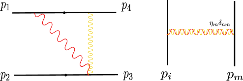
Figure 1: Scattering process due to soft graviton exchanges involving a double graviton vertex and two single graviton Weinberg vertices. The particles with a double graviton vertex are labeled by the index $i$ and the ones with a single graviton vertex by $n$ and $m$. The left subfigure is a general diagram with $n\neq m$, which is inconsistent with the collinear requirement on the double graviton vertex. The right subfigure is our resolution by requiring $n=m$, which collapses the two Weinberg vertices into one by implementing an additional factor $\eta_{m}\delta_{nm}$.

There are several avenues for future research. One involves performing the sums described above to derive 4PM and higher gravitational wave observables. The analysis can be carried out along similar lines as those for the Weinberg soft factor dressing for eikonal amplitudes in [30]. This, in particular, involves substituting expressions for the relative velocities $\sigma_{ab}$ in terms of the PM expansion for the impulse following eikonal kinematics. It will also be interesting to consider the implications of the quadratic graviton mode operator $e^{-\Delta_{2}}$ in 42 for gravitationally interacting bodies more generally. One can expect, due to its similarity with a squeezing operator in squeezed coherent states, that it contributes to super-Poissonian statistics. In addition, we note that entanglement entropy can be used to constrain scattering amplitudes [99, 100, 101, 102] and more specifically amplitudes with a Weinberg soft graviton dressing [103, 104, 105]. It will be interesting to investigate the role of non-linear graviton mode dressings on these results.

Acknowledgement :

We would like to thank Filippo Vernizzi, Chia-Hsien Shen and Yu-tin Huang for their valuable feedback on our preliminary results. FLL thanks the hospitality of the organizers of the workshop ”Gravitational waves meet effective field theories” held at Benasque, Spain on Aug 20-26 of 2023, during which he presented an earlier version of this work. The work of KF is supported by Taiwan’s NSTC with grant numbers 111-2811-M-003-005 and 112-2811-M-003 -003-MY3. The work of FLL is supported by Taiwan’s NSTC with grant numbers 109-2112-M-003-007-MY3 and 112-2112-M-003-006-MY3. We also like to thank the support of iCAG funding by NTNU.

Appendix A General form of factorized gravitational dressing

This Appendix provides a detailed derivation of 42 to all orders in $\kappa$. We further consider the evolution of creation and annihilation modes by the dressing operator, which can be used to compute observables.

Given the operator $\exp[-\tilde{\Delta}_{1}-\Delta_{2}]$ we first require that it be equivalent to another operator $\exp[-\bar{\Delta}]\exp[-\Delta_{2}]$. This implies that

$$\exp[-\bar{\Delta}]=\exp[-\tilde{\Delta}_{1}-\Delta_{2}]\exp[\Delta_{2}]\;,$$ (158)

where $\bar{\Delta}$ can now be determined by using the BCH formula. To simplify notation, we adopt the letter notation for nested commutator,

$$\left[X_{1}\,,\left[X_{2}\,,\left[X_{3}\left[X_{4}\,,\left[X_{5}\,,\cdots\right]\right]\right]\right]\right]=\left[X_{1}X_{2}X_{3}X_{4}X_{5}\cdots\right]\;.$$ (159)

The BCH formula expanded to the first five orders takes the form [106]

$$\ln\left(\exp[X]\exp[Y]\right) =X+Y+\frac{1}{2}[XY]+\frac{1}{12}[(X-Y)XY]-\frac{1}{24}[XYXY]+\frac{1}{6!}\left(-[X^{4}Y]-[Y^{4}X]\right.$$

$$\left.\qquad\quad+2[XY^{3}X]+2[YX^{3}Y]+6[YXYXY]+6[XYXYX]\right)+\cdots\;.$$ (160)

We apply this in 158 by taking $X=-\tilde{\Delta}_{1}-\Delta_{2}$ and $Y=\Delta_{2}$. This gives

$$-\bar{\Delta} =\ln\left(\exp[-\tilde{\Delta}_{1}-\Delta_{2}]\exp[\Delta_{2}]\right)\;,$$

$$=-\tilde{\Delta}_{1}+\frac{1}{2}\left[\Delta_{2}\tilde{\Delta}_{1}\right]-\frac{1}{12}\left[(\tilde{\Delta}_{1}+2\Delta_{2})\Delta_{2}\tilde{\Delta}_{1}\right]+\frac{1}{24}\left[(\tilde{\Delta}_{1}+\Delta_{2})\Delta_{2}^{2}\tilde{\Delta}_{1}\right]$$

$$\qquad+\frac{1}{6!}\left(\left[(\tilde{\Delta}_{1}+2\Delta_{2})^{3}\Delta_{2}\tilde{\Delta}_{1}\right]-6\left[(\tilde{\Delta}_{1}+2\Delta_{2})\Delta_{2}(\tilde{\Delta}_{1}+2\Delta_{2})\Delta_{2}\tilde{\Delta}_{1}\right]+2\left[(\tilde{\Delta}_{1}+2\Delta_{2})\Delta_{2}^{3}\tilde{\Delta}_{1}\right]\right.$$

$$\left.\qquad\qquad\quad+2\left[\Delta_{2}(\tilde{\Delta}_{1}+2\Delta_{2})^{2}\Delta_{2}\tilde{\Delta}_{1}\right]-6\left[\Delta_{2}(\tilde{\Delta}_{1}+2\Delta_{2})\Delta_{2}^{2}\tilde{\Delta}_{1}\right]+\left[\Delta_{2}^{4}\tilde{\Delta}_{1}\right]\right)+\cdots\;.$$ (161)

The series in 161 simplifies into a sum over two terms. Those with $\left[\Delta_{2}^{n}\tilde{\Delta}_{1}\right]$ for all $n\geq 0$, which is a single graviton state of the form $\tilde{\Delta}_{1}$ but with different coefficients for the graviton creation and annihilation modes. The only contributions involving more than one $\tilde{\Delta}_{1}$ in the nested commutators is of the form $\left[\tilde{\Delta}_{1}\Delta_{2}^{n}\tilde{\Delta}_{1}\right]$, which involve no graviton modes. We find that 161 can be expressed as

$$-\bar{\Delta} =-\Delta_{1}-\Delta_{0}$$

$$\Delta_{1} =\tilde{\Delta}_{1}+\sum_{n=1}^{\infty}\frac{(-1)^{n}}{(n+1)!}\left[\Delta_{2}^{n}\tilde{\Delta}_{1}\right]$$ (162)

$$\Delta_{0} =\sum_{n=1}^{\infty}c_{n}\frac{(-1)^{n+1}}{(n+2)!}\left[\tilde{\Delta}_{1}\Delta_{2}^{n}\tilde{\Delta}_{1}\right]\,,$$ (163)

where we have explicitly separated the $n=0$ contribution in $\Delta_{1}$, which is the single graviton term of the unfactorized gravitational dressing. We hence find that $-\bar{\Delta}$ can be written as a sum over a single graviton mode and a zero graviton factor known up to certain constants $c_{n}$, with the first few constants being $c_{1}=\frac{1}{2}\,,c_{2}=1\,,c_{3}=\frac{1}{2}\,,c_{4}=\frac{3}{2}\,,\cdots$. However, in the following, we show that $\Delta_{0}$ vanishes, and hence the dressing $\exp[-\bar{\Delta}]$ can be written as a normalized single graviton dressing. We also note that since $\tilde{\Delta}_{1}$ and $\Delta_{2}$ are respectively ${\cal O}(\kappa)$ and ${\cal O}(\kappa^{2})$, 162 provides a single graviton (coherent) dressing to ${\cal O}(\kappa^{2n+1})$ for all positive integers $n$.

Using the expressions for $\Delta_{2}$ and $\tilde{\Delta}_{1}$, we determine the following result for $\Delta_{1}$ and $\Delta_{0}$

$$\Delta_{1} =\frac{1}{\hbar}\int_{\vec{k}}d^{3}k\left(a_{i}(k)f^{*}_{i}(k)-a^{\dagger}_{i}(k)f_{i}(k)\right)$$

$$\qquad+\frac{1}{\hbar}\int_{\vec{l}}d^{3}l\int_{\vec{k}}d^{3}ka_{i}(k)\left[\sum_{n=1}^{\infty}\frac{1}{(n+1)!}\left(\mathcal{C}_{ij;n}^{*}(k\,,l)f^{*}_{j}(l)-\mathcal{S}_{ij;n}^{*}(k\,,l)f_{j}(l)\right)\right]$$

$$\qquad\qquad-\frac{1}{\hbar}\int_{\vec{l}}d^{3}l\int_{\vec{k}}d^{3}ka^{\dagger}_{i}(k)\left[\sum_{n=1}^{\infty}\frac{1}{(n+1)!}\left(\mathcal{C}_{ij;n}(k\,,l)f_{j}(l)-\mathcal{S}_{ij;n}(k\,,l)f^{*}_{j}(l)\right)\right]\,,$$ (164)

$$\Delta_{0} =\frac{1}{\hbar}\int_{\vec{l}}d^{3}l\int_{\vec{k}}d^{3}k\left[\sum_{n=1}^{\infty}\frac{c_{n}}{(n+2)!}\left(f^{*}_{i}(k)\mathcal{C}_{ij;n}(k\,,l)f_{j}(l)-f_{i}(k)\mathcal{C}_{ij;n}^{*}(k\,,l)f^{*}_{j}(l)\phantom{\sum_{n}\frac{c_{n}}{(n+2)!}}\right.\right.$$

$$\left.\left.\quad\qquad\qquad\qquad\qquad\phantom{\sum_{n}\frac{c_{n}}{(n+2)!}}+f_{i}(k)\mathcal{S}_{ij;n}^{*}(k\,,l)f_{j}(l)-f^{*}_{i}(k)\mathcal{S}_{ij;n}(k\,,l)f^{*}_{j}(l)\right)\right]$$ (165)

with $\mathcal{S}_{ij;n}(k\,,l)$ and $\mathcal{C}_{ij;n}(k\,,l)$ defined in terms of a products over an integrated expression $I^{(\pm)\mu_{m}\nu_{m}}_{\mu_{m+1}\nu_{m+1}}(l_{m+1})$

$$S_{ij;n}(k\,,l) =\frac{1}{2}\int_{\vec{l}_{n}}d^{3}l_{n}\,\varepsilon^{*}_{i\,,\mu_{0}\nu_{0}}(l_{0})\,\varepsilon_{j}^{*\;\mu_{n}\nu_{n}}(l_{n})\,\delta(\vec{l_{0}}\,,\vec{k})\,\delta(\vec{l_{n}}\,,\vec{l})$$

$$\qquad\qquad\left[\left(\prod_{m=0}^{n-1}I^{(-)\mu_{m}\nu_{m}}_{\mu_{m+1}\nu_{m+1}}(l_{m+1})\right)+(-1)^{n+1}\left(\prod_{m=0}^{n-1}I^{(+)\mu_{m}\nu_{m}}_{\mu_{m+1}\nu_{m+1}}(l_{m+1})\right)\right]\;,$$ (166)

$$C_{ij;n}(k\,,l) =\frac{1}{2}\int_{\vec{l}_{n}}d^{3}l_{n}\,\varepsilon^{*}_{i\,,\mu_{0}\nu_{0}}(l_{0})\,\varepsilon_{j}^{\mu_{n}\nu_{n}}(l_{n})\,\delta(\vec{l_{0}}\,,\vec{k})\,\delta(\vec{l_{n}}\,,\vec{l})$$

$$\qquad\qquad\left[\left(\prod_{m=0}^{n-1}I^{(-)\mu_{m}\nu_{m}}_{\mu_{m+1}\nu_{m+1}}(l_{m+1})\right)+(-1)^{n}\left(\prod_{m=0}^{n-1}I^{(+)\mu_{m}\nu_{m}}_{\mu_{m+1}\nu_{m+1}}(l_{m+1})\right)\right]\;,$$ (167)

$$I^{(\pm)\mu_{m}\nu_{m}}_{\mu_{m+1}\nu_{m+1}}(l_{m+1}) =\int_{\vec{l}_{m}}d^{3}l_{m}\,\Pi^{\mu_{m}\nu_{m}}_{\alpha_{m}\beta_{m}}(l_{m})\Pi^{\alpha_{m+1}\beta_{m+1}}_{\mu_{m+1}\nu_{m+1}}(l_{m+1})$$

$$\qquad\qquad\qquad\left[A^{\alpha_{m}\beta_{m}}_{\alpha_{m+1}\beta_{m+1}}(l_{m}\,,l_{m+1})\pm B^{\alpha_{m}\beta_{m}}_{\alpha_{m+1}\beta_{m+1}}(l_{m}\,,l_{m+1})\right]\;.$$ (168)

As the integrals in 165 are not sensitive to the poles of $\omega_{k}$ and $\omega_{l}$, we have $\Delta_{0}=0$. We conclude with the general expressions for $e^{\Delta}a_{i}(k)e^{-\Delta}$ and $e^{\Delta}a_{i}^{\dagger}(k)e^{-\Delta}$ to all orders in $\kappa$

$$e^{\Delta}a_{i}(k)e^{-\Delta} =a_{i}(k)+f_{i}(k)$$

$$\qquad+\frac{1}{\hbar}\int_{\vec{l}}d^{3}l\int_{\vec{k}}d^{3}k\left[\sum_{n=1}^{\infty}\frac{1}{(n+1)!}\left(\mathcal{C}_{ij;n}(k\,,l)f_{j}(l)-\mathcal{S}_{ij;n}(k\,,l)f^{*}_{j}(l)\right)\right]$$

$$\qquad\qquad\quad+\frac{1}{\hbar}\int_{\vec{l}}d^{3}l\int_{\vec{k}}d^{3}k\left[\sum_{n=1}^{\infty}\frac{1}{n!}\left(\mathcal{C}_{ij;n}(k\,,l)a_{j}(l)-\mathcal{S}_{ij;n}(k\,,l)a^{\dagger}_{j}(l)\right)\right]$$ (169)

$$e^{\Delta}a^{\dagger}_{i}(k)e^{-\Delta} =a^{\dagger}_{i}(k)+f^{*}_{i}(k)$$

$$\qquad+\frac{1}{\hbar}\int_{\vec{l}}d^{3}l\int_{\vec{k}}d^{3}k\left[\sum_{n=1}^{\infty}\frac{1}{(n+1)!}\left(\mathcal{C}_{ij;n}^{*}(k\,,l)f^{*}_{j}(l)-\mathcal{S}_{ij;n}^{*}(k\,,l)f_{j}(l)\right)\right]$$

$$\qquad\qquad\quad+\frac{1}{\hbar}\int_{\vec{l}}d^{3}l\int_{\vec{k}}d^{3}k\left[\sum_{n=1}^{\infty}\frac{1}{n!}\left(\mathcal{C}_{ij;n}^{*}(k\,,l)a^{\dagger}_{j}(l)-\mathcal{S}_{ij;n}^{*}(k\,,l)a_{j}(l)\right)\right]\;.$$ (170)

This is the all order generalization of the $n=1$ (${\cal O}(\kappa^{3})$) correction result in 45 and 46.

Appendix B Evaluation of $F_{inm}$ and $\vec{G}_{inm}$

In the following, we will always consider the graviton orientation to be given by

$$\hat{k}=\left(\sqrt{1-y^{2}}\cos\phi\,,\sqrt{1-y^{2}}\sin\phi\,,y\right)\,,$$ (171)

with $y=\cos\theta$ . The parameterizations adopted for $\vec{p}_{n}\,,\vec{p}_{m}$ and $\vec{p}_{i}$ in the two subsections will be treated differently. We will however always use the freedom to have all the hard particle momenta in a $2$-dimensional plane, which we consider along the ‘x-z’ plane throughout. The integrals we consider will also have a non-trivial integration over $\phi$, and will make use of the following result

$$\int_{0}^{2\pi}d\phi\frac{1}{A+B\cos\phi}=\frac{2\pi}{\sqrt{A^{2}-B^{2}}}\;.$$ (172)

B.1 Evaluation of $F_{inm}$

We consider the following parametrization for the external particle spatial momenta

$$\vec{p}_{n}=\left(0\,,0\,,\bar{p}_{n}\right)\;,\; \;\vec{p}_{i}=\left(-\bar{p}_{m}\,,0\,,-\bar{p}_{n}\right)\;,\;\;\vec{p}_{m}=\left(\bar{p}_{m}\,,0\,,0\right)\;,$$ (173)

which satisfy the conservation of momentum: $\vec{p}_{n}+\vec{p}_{i}+\vec{p}_{m}=0$

We then have the following integral for 111

$$F_{inm} :=\frac{1}{2\pi}\oint d\Omega_{k}\frac{1}{(E_{n}-\vec{p}_{n}.\hat{k})(E_{i}-\vec{p}_{i}.\hat{k})(E_{m}-\vec{p}_{m}.\hat{k})}\,,$$

$$=\frac{1}{2\pi}\int_{-1}^{1}dy\frac{1}{(E_{n}-\bar{p}_{n}y)}\int_{0}^{2\pi}d\phi\frac{1}{(E_{i}+\bar{p}_{n}y+\bar{p}_{m}\sqrt{1-y^{2}}\cos\phi)(E_{m}-\bar{p}_{m}\sqrt{1-y^{2}}\cos\phi)}$$

$$=\frac{1}{2\pi}\int_{-1}^{1}dy\frac{1}{(E_{n}-\bar{p}_{n}y)(E_{i}+E_{m}+\bar{p}_{n}y)}$$

$$\qquad\qquad\int_{0}^{2\pi}d\phi\left[\frac{1}{E_{i}+\bar{p}_{n}y+\bar{p}_{m}\sqrt{1-y^{2}}\cos\phi}+\frac{1}{E_{m}-\bar{p}_{m}\sqrt{1-y^{2}}\cos\phi}\right]$$ (174)

Applying 172 in 174 gives

$$F_{inm} =\int_{-1}^{1}dy\frac{1}{(E_{n}-\bar{p}_{n}y)(E_{i}+E_{m}+\bar{p}_{n}y)}\left[\frac{1}{\sqrt{(E_{i}+\bar{p}_{n}y)^{2}-\bar{p}_{m}^{2}(1-y^{2})}}+\frac{1}{\sqrt{E_{m}^{2}-\bar{p}_{m}^{2}(1-y^{2})}}\right]$$

$$=\frac{1}{E_{i}+E_{m}+E_{n}}\left[\frac{1}{\sqrt{E_{n}^{2}E_{m}^{2}-m_{m}^{2}m_{n}^{2}}}\ln\left(\frac{E_{m}E_{n}+\sqrt{E_{n}^{2}E_{m}^{2}-m_{m}^{2}m_{n}^{2}}}{E_{m}E_{n}-\sqrt{E_{n}^{2}E_{m}^{2}-m_{m}^{2}m_{n}^{2}}}\right)\right.$$

$$\left.\qquad+\frac{1}{\sqrt{(E_{i}+E_{n})^{2}\bar{p}_{n}^{2}+m_{n}^{2}\bar{p}_{m}^{2}}}\ln\left(\frac{E_{i}E_{n}+\bar{p}_{n}^{2}+\sqrt{(E_{i}+E_{n})^{2}\bar{p}_{n}^{2}+m_{n}^{2}\bar{p}_{m}^{2}}}{E_{i}E_{n}+\bar{p}_{n}^{2}-\sqrt{(E_{i}+E_{n})^{2}\bar{p}_{n}^{2}+m_{n}^{2}\bar{p}_{m}^{2}}}\right)\right.$$

$$\left.\qquad\quad+\frac{1}{\sqrt{(E_{i}+E_{m})^{2}\bar{p}_{m}^{2}+m_{m}^{2}\bar{p}_{n}^{2}}}\ln\left(\frac{E_{i}E_{m}+\bar{p}_{m}^{2}+\sqrt{(E_{i}+E_{m})^{2}\bar{p}_{m}^{2}+m_{m}^{2}\bar{p}_{n}^{2}}}{E_{i}E_{m}+\bar{p}_{m}^{2}-\sqrt{(E_{i}+E_{m})^{2}\bar{p}_{m}^{2}+m_{m}^{2}\bar{p}_{n}^{2}}}\right)\right]$$ (175)

From 62 and $-p_{a}^{2}=E_{a}^{2}-\vec{p}_{a}^{2}=m_{a}^{2}$ for $a=n,m,i$, we then find that the parametrization 173 gives the following relations

$$E_{m}E_{n}=m_{m}m_{n}\sigma_{mn} \,,\qquad\qquad E_{n}^{2}E_{m}^{2}-m_{m}^{2}m_{n}^{2}=m_{m}^{2}m_{n}^{2}\left(\sigma_{mn}^{2}-1\right)\;,$$

$$E_{i}E_{m}+\bar{p}_{m}^{2}=m_{i}m_{m}\sigma_{im} \,,\qquad\qquad(E_{i}+E_{m})^{2}\bar{p}_{m}^{2}+m_{m}^{2}\bar{p}_{n}^{2}=m_{i}^{2}m_{m}^{2}\left(\sigma_{im}^{2}-1\right)\;,$$

$$E_{i}E_{n}+\bar{p}_{n}^{2}=m_{i}m_{n}\sigma_{in} \,,\qquad\qquad(E_{i}+E_{n})^{2}\bar{p}_{n}^{2}+m_{n}^{2}\bar{p}_{m}^{2}=m_{n}^{2}m_{i}^{2}\left(\sigma_{in}^{2}-1\right)\;,$$

$$E_{i}+E_{m}+E_{n} =\sqrt{2(m_{m}m_{n}\sigma_{mn}+m_{i}m_{m}\sigma_{im}+m_{i}m_{n}\sigma_{in})+m_{i}^{2}+m_{m}^{2}+m_{n}^{2}}\;.$$ (176)

Substituting 176 in 175, we get the result

$$F_{inm} =\frac{2\;(m_{i}\Delta_{mn}+m_{n}\Delta_{im}+m_{m}\Delta_{ni})}{m_{n}m_{i}m_{m}\sqrt{2(m_{m}m_{n}\sigma_{mn}+m_{i}m_{m}\sigma_{im}+m_{i}m_{n}\sigma_{in})+m_{i}^{2}+m_{m}^{2}+m_{n}^{2}}}\;,$$ (177)

where $\Delta_{ab}$ is defined in 62.

B.2 Evaluation of $\vec{G}_{inm}$

We now consider the derivation of 112. Start with the following decomposition:

$$\vec{G}_{inm}:={1\over 2\pi}\oint d\Omega_{k}\frac{\hat{k}}{(E_{i}-\vec{p}_{i}.\hat{k})(E_{n}-\vec{p}_{n}.\hat{k})(E_{m}-\vec{p}_{m}.\hat{k})}:=a_{nim}\hat{p}_{n}+b_{nim}\hat{p}_{m}+c_{nim}\hat{p}_{i}\,.$$ (178)

In the above, we used the rotational symmetry of the integral to express it as a linear combination over the hard particle orientations in the last equality. Defining $\hat{p}_{m}\cdot\hat{p}_{n}=\cos\theta_{mn}$ as the relative angle between two hard particle orientations $\hat{p}_{m}$ and $\hat{p}_{n}$, we then find the following solutions for $a_{nim}\,,b_{nim}$ and $c_{nim}$ from 178

$$a_{nim} =\frac{\vec{G}\cdot\hat{p}_{n}\sin^{2}\theta_{im}+\cos\theta_{im}\left(\vec{G}\cdot\hat{p}_{m}\cos\theta_{ni}+\vec{G}\cdot\hat{p}_{i}\cos\theta_{nm}\right)-\left(\vec{G}\cdot\hat{p}_{i}\cos\theta_{ni}+\vec{G}\cdot\hat{p}_{m}\cos\theta_{nm}\right)}{1+2\cos\theta_{nm}\cos\theta_{ni}\cos\theta_{im}-\cos^{2}\theta_{nm}-\cos^{2}\theta_{ni}-\cos^{2}\theta_{im}}$$

$$b_{nim} =\frac{\vec{G}\cdot\hat{p}_{m}\sin^{2}\theta_{ni}+\cos\theta_{ni}\left(\vec{G}\cdot\hat{p}_{n}\cos\theta_{im}+\vec{G}\cdot\hat{p}_{i}\cos\theta_{nm}\right)-\left(\vec{G}\cdot\hat{p}_{i}\cos\theta_{im}+\vec{G}\cdot\hat{p}_{n}\cos\theta_{nm}\right)}{1+2\cos\theta_{nm}\cos\theta_{ni}\cos\theta_{im}-\cos^{2}\theta_{nm}-\cos^{2}\theta_{ni}-\cos^{2}\theta_{im}}$$

$$c_{nim} =\frac{\vec{G}\cdot\hat{p}_{i}\sin^{2}\theta_{nm}+\cos\theta_{nm}\left(\vec{G}\cdot\hat{p}_{n}\cos\theta_{im}+\vec{G}\cdot\hat{p}_{m}\cos\theta_{ni}\right)-\left(\vec{G}\cdot\hat{p}_{m}\cos\theta_{im}+\vec{G}\cdot\hat{p}_{n}\cos\theta_{ni}\right)}{1+2\cos\theta_{nm}\cos\theta_{ni}\cos\theta_{im}-\cos^{2}\theta_{nm}-\cos^{2}\theta_{ni}-\cos^{2}\theta_{im}}$$ (179)

In the above, we have omitted the sub-indices of $\vec{G}_{inm}$ to avoid clutter of expressions.

Thus, the expression for $\vec{G}_{inm}$ is completely specified from its contraction with the hard particle orientations. In the following, we consider the derivation for

$$\vec{G}_{inm}\cdot\hat{p}_{a}=\frac{1}{2\pi}\oint d\Omega_{k}\frac{\hat{p}_{a}\cdot\hat{k}}{(E_{i}-\vec{p}_{i}\cdot\hat{k})(E_{n}-\vec{p}_{n}\cdot\hat{k})(E_{m}-\vec{p}_{m}\cdot\hat{k})}\,,$$ (180)

which cover the cases for $a=i,n,m$ by an appropriate choice of indices. We can carry out the integration using the parametrization

$$\vec{p}_{n}=\bar{p}_{n}\hat{p}_{n}\;; \qquad\hat{p}_{n}=\left(0\,,0\,,1\right)\,,$$

$$\vec{p}_{i}=\bar{p}_{i}\hat{p}_{i}\;; \qquad\hat{p}_{i}=\left(\sin\theta_{ni}\,,0\,,\cos\theta_{ni}\right)\,,$$

$$\vec{p}_{m}=\bar{p}_{m}\hat{p}_{m}\;; \qquad\hat{p}_{m}=\left(\sin\theta_{nm}\,,0\,,\cos\theta_{nm}\right)\,,$$ (181)

With this parametrization, we have the following Lorentz invariant quantities

$$\sigma_{ab}=\frac{E_{a}E_{b}-\bar{p}_{a}\bar{p}_{b}\cos\theta_{ab}}{m_{a}m_{b}}\,,\quad\sigma_{ac}=\frac{E_{a}E_{c}-\bar{p}_{a}\bar{p}_{c}\cos\theta_{ac}}{m_{a}m_{c}}\,,\qquad\sigma_{bc}=\frac{E_{b}E_{c}-\bar{p}_{b}\bar{p}_{c}\cos(\theta_{ac}-\theta_{ab})}{m_{b}m_{c}}\,,$$

$$m_{a}^{2}m_{c}^{2}\left(\sigma_{ac}^{2}-1\right)=E_{a}^{2}\bar{p}_{c}^{2}+E_{c}^{2}\bar{p}_{a}^{2}-2E_{a}E_{c}\bar{p}_{a}\bar{p}_{c}\cos\theta_{ac}-\bar{p}_{a}^{2}\bar{p}_{c}^{2}\sin^{2}\theta_{ac}\,,$$

$$m_{a}^{2}m_{b}^{2}\left(\sigma_{ab}^{2}-1\right)=E_{a}^{2}\bar{p}_{b}^{2}+E_{b}^{2}\bar{p}_{a}^{2}-2E_{a}E_{b}\bar{p}_{a}\bar{p}_{b}\cos\theta_{ab}-\bar{p}_{a}^{2}\bar{p}_{b}^{2}\sin^{2}\theta_{ab}\,,$$

$$m_{b}^{2}m_{c}^{2}\left(\sigma_{bc}^{2}-1\right)=E_{c}^{2}\bar{p}_{b}^{2}+E_{b}^{2}\bar{p}_{c}^{2}-2E_{b}E_{c}\bar{p}_{b}\bar{p}_{c}\cos(\theta_{ac}-\theta_{ab})-\bar{p}_{b}^{2}\bar{p}_{c}^{2}\sin^{2}(\theta_{ac}-\theta_{ab})\,.$$ (182)

Using 181 and 171 in 180, we have

$$\vec{G}_{inm}\cdot\hat{p}_{a} =\frac{1}{\pi}\int_{-1}^{1}dy\frac{y}{(E_{a}-\bar{p}_{a}y)}$$

$$\quad\int_{0}^{\pi}d\phi\frac{1}{(E_{b}-\bar{p}_{b}(\cos\theta_{ab}y+\sin\theta_{ab}\sqrt{1-y^{2}}\cos\phi))(E_{c}-\bar{p}_{c}(\cos\theta_{ac}y+\sin\theta_{ac}\sqrt{1-y^{2}}\cos\phi))}$$

$$=\int_{-1}^{1}dy\frac{y}{(E_{a}-\bar{p}_{a}y)((E_{b}\bar{p}_{c}\sin\theta_{ac}-E_{c}\bar{p}_{b}\sin\theta_{ab})+y\bar{p}_{c}\bar{p}_{b}(\cos\theta_{ac}\sin\theta_{ab}-\cos\theta_{ab}\sin\theta_{ac}))}$$

$$\left[\frac{\bar{p}_{c}\sin\theta_{ac}}{(E_{c}-\bar{p}_{c}\cos\theta_{ac}y)^{2}-\bar{p}^{2}_{c}(1-y^{2})\sin^{2}\theta_{ac}}-\frac{\bar{p}_{b}\sin\theta_{ab}}{(E_{b}-\bar{p}_{b}\cos\theta_{ab}y)^{2}-\bar{p}^{2}_{b}(1-y^{2})\sin^{2}\theta_{ab}}\right]$$ (183)

where we used 172 to arrive at the last line of 183. The $y$ integral can be evaluated to find a result that depends on the Lorentz invariant quatities, as well as on $\{\frac{E_{a}}{m_{a}}\,,\frac{E_{b}}{m_{b}}\,,\frac{E_{c}}{m_{c}}\}$ and $\frac{\bar{p}_{a}}{m_{a}}$. Defining

$$\gamma^{(a)}_{bc}:=\frac{m_{a}}{\bar{p}_{a}}\left(\frac{E_{b}}{m_{b}}\sigma_{ab}-\frac{E_{c}}{m_{c}}\sigma_{ac}\right)\,, \qquad\chi^{(a)}_{ab}:=\sqrt{\sigma_{ab}^{2}-1+\left(\frac{E_{b}^{2}}{m_{b}^{2}}+\frac{E_{a}^{2}}{m_{a}^{2}}-2\frac{E_{a}}{m_{a}}\frac{E_{b}}{m_{b}}\sigma_{ab}\right)}\,,$$

$$\Delta^{(a)}_{abc} :=\chi^{(a)}_{ac}\gamma^{(a)}_{ba}-\chi^{(a)}_{ab}\gamma^{(a)}_{ca}\,,$$

$$\alpha^{(a)}_{bc}:=\sigma_{bc}-\frac{\chi^{(a)}_{ab}}{\chi^{(a)}_{ac}}\,, \qquad\beta^{(a)}_{bc}:=\sigma_{bc}-\frac{\chi^{(a)}_{ac}}{\chi^{(a)}_{ab}}\,;\qquad\qquad(b\,,c\neq a)\,,$$

$$\xi^{(a)}_{ab}:=\frac{\sigma_{ab}^{2}-1+\gamma^{(a)}_{ba}\sqrt{\sigma_{ab}^{2}-1}}{\sigma_{ab}\left(\gamma^{(a)}_{ba}+\sqrt{\sigma_{ab}^{2}-1}\right)}\,, \qquad\xi^{(a)}_{ac}:=\frac{\sigma_{ac}^{2}-1+\gamma^{(a)}_{ca}\sqrt{\sigma_{ac}^{2}-1}}{\sigma_{ac}\left(\gamma^{(a)}_{ca}+\sqrt{\sigma_{ac}^{2}-1}\right)}\,,$$

$$\mu^{(a)}_{bc}:=\frac{\sigma_{bc}^{2}-1+\gamma^{(a)}_{bc}\sqrt{\sigma_{bc}^{2}-1}}{\alpha^{(a)}_{bc}\left(\gamma^{(a)}_{bc}+\sqrt{\sigma_{bc}^{2}-1}\right)}\,, \qquad\nu^{(a)}_{bc}:=\frac{\sigma_{bc}^{2}-1+\gamma^{(a)}_{bc}\sqrt{\sigma_{bc}^{2}-1}}{\beta^{(a)}_{bc}\left(\gamma^{(a)}_{bc}+\sqrt{\sigma_{bc}^{2}-1}\right)}\,,$$ (184)

we find that 183 has the result

$$\vec{G}_{inm}\cdot\hat{p}_{a} =\frac{2}{m_{a}m_{b}m_{c}}\frac{1}{\Delta^{(a)}_{abc}}\left[\chi^{(a)}_{ac}\left(\frac{E_{a}}{m_{a}}\frac{\operatorname{arctanh}\xi^{(a)}_{ac}}{\sqrt{\sigma_{ac}^{2}-1}}-\frac{E_{b}}{m_{b}}\frac{\operatorname{arctanh}\mu^{(a)}_{bc}+\operatorname{arctanh}\nu^{(a)}_{bc}}{\sqrt{\sigma_{bc}^{2}-1}}\right)\right.$$

$$\left.\quad\qquad\qquad\qquad\qquad-\chi^{(a)}_{ab}\left(\frac{E_{a}}{m_{a}}\frac{\operatorname{arctanh}\xi^{(a)}_{ab}}{\sqrt{\sigma_{ab}^{2}-1}}-\frac{E_{c}}{m_{c}}\frac{\operatorname{arctanh}\mu^{(a)}_{bc}+\operatorname{arctanh}\nu^{(a)}_{bc}}{\sqrt{\sigma_{bc}^{2}-1}}\right)\right]\;.$$ (185)

References

• [1] W.D. Goldberger and I.Z. Rothstein, An Effective field theory of gravity for extended objects, Phys. Rev. D 73 (2006) 104029 [hep-th/0409156].
• [2] W.D. Goldberger and A.K. Ridgway, Radiation and the classical double copy for color charges, Phys. Rev. D 95 (2017) 125010 [1611.03493].
• [3] T. Damour, Gravitational scattering, post-Minkowskian approximation and Effective One-Body theory, Phys. Rev. D 94 (2016) 104015 [1609.00354].
• [4] A. Luna, R. Monteiro, I. Nicholson, D. O’Connell and C.D. White, The double copy: Bremsstrahlung and accelerating black holes, JHEP 06 (2016) 023 [1603.05737].
• [5] A. Luna, I. Nicholson, D. O’Connell and C.D. White, Inelastic Black Hole Scattering from Charged Scalar Amplitudes, JHEP 03 (2018) 044 [1711.03901].
• [6] N.E.J. Bjerrum-Bohr, P.H. Damgaard, G. Festuccia, L. Planté and P. Vanhove, General Relativity from Scattering Amplitudes, Phys. Rev. Lett. 121 (2018) 171601 [1806.04920].
• [7] C. Cheung, I.Z. Rothstein and M.P. Solon, From Scattering Amplitudes to Classical Potentials in the Post-Minkowskian Expansion, Phys. Rev. Lett. 121 (2018) 251101 [1808.02489].
• [8] D.A. Kosower, B. Maybee and D. O’Connell, Amplitudes, Observables, and Classical Scattering, JHEP 02 (2019) 137 [1811.10950].
• [9] A. Cristofoli, N.E.J. Bjerrum-Bohr, P.H. Damgaard and P. Vanhove, Post-Minkowskian Hamiltonians in general relativity, Phys. Rev. D 100 (2019) 084040 [1906.01579].
• [10] N.E.J. Bjerrum-Bohr, A. Cristofoli and P.H. Damgaard, Post-Minkowskian Scattering Angle in Einstein Gravity, JHEP 08 (2020) 038 [1910.09366].
• [11] G. Mogull, J. Plefka and J. Steinhoff, Classical black hole scattering from a worldline quantum field theory, JHEP 02 (2021) 048 [2010.02865].
• [12] P.H. Damgaard, L. Plante and P. Vanhove, On an exponential representation of the gravitational S-matrix, JHEP 11 (2021) 213 [2107.12891].
• [13] S. Caron-Huot, M. Giroux, H.S. Hannesdottir and S. Mizera, What can be measured asymptotically?, 2308.02125.
• [14] Z. Bern, C. Cheung, R. Roiban, C.-H. Shen, M.P. Solon and M. Zeng, Scattering Amplitudes and the Conservative Hamiltonian for Binary Systems at Third Post-Minkowskian Order, Phys. Rev. Lett. 122 (2019) 201603 [1901.04424].
• [15] Z. Bern, C. Cheung, R. Roiban, C.-H. Shen, M.P. Solon and M. Zeng, Black Hole Binary Dynamics from the Double Copy and Effective Theory, JHEP 10 (2019) 206 [1908.01493].
• [16] T. Damour, Classical and quantum scattering in post-Minkowskian gravity, Phys. Rev. D 102 (2020) 024060 [1912.02139].
• [17] Z. Bern, H. Ita, J. Parra-Martinez and M.S. Ruf, Universality in the classical limit of massless gravitational scattering, Phys. Rev. Lett. 125 (2020) 031601 [2002.02459].
• [18] G. Kälin, Z. Liu and R.A. Porto, Conservative Dynamics of Binary Systems to Third Post-Minkowskian Order from the Effective Field Theory Approach, Phys. Rev. Lett. 125 (2020) 261103 [2007.04977].
• [19] J. Parra-Martinez, M.S. Ruf and M. Zeng, Extremal black hole scattering at $\mathcal{O}(G^{3})$: graviton dominance, eikonal exponentiation, and differential equations, JHEP 11 (2020) 023 [2005.04236].
• [20] T. Damour, Radiative contribution to classical gravitational scattering at the third order in $G$, Phys. Rev. D 102 (2020) 124008 [2010.01641].
• [21] E. Herrmann, J. Parra-Martinez, M.S. Ruf and M. Zeng, Gravitational Bremsstrahlung from Reverse Unitarity, Phys. Rev. Lett. 126 (2021) 201602 [2101.07255].
• [22] S. Mougiakakos, M.M. Riva and F. Vernizzi, Gravitational Bremsstrahlung in the post-Minkowskian effective field theory, Phys. Rev. D 104 (2021) 024041 [2102.08339].
• [23] E. Herrmann, J. Parra-Martinez, M.S. Ruf and M. Zeng, Radiative classical gravitational observables at $\mathcal{O}$(G3) from scattering amplitudes, JHEP 10 (2021) 148 [2104.03957].
• [24] P. Di Vecchia, C. Heissenberg, R. Russo and G. Veneziano, The eikonal approach to gravitational scattering and radiation at $\mathcal{O}$(G3), JHEP 07 (2021) 169 [2104.03256].
• [25] D. Bini, T. Damour and A. Geralico, Radiative contributions to gravitational scattering, Phys. Rev. D 104 (2021) 084031 [2107.08896].
• [26] P. Di Vecchia, C. Heissenberg, R. Russo and G. Veneziano, The eikonal operator at arbitrary velocities I: the soft-radiation limit, JHEP 07 (2022) 039 [2204.02378].
• [27] G. Kälin, J. Neef and R.A. Porto, Radiation-reaction in the Effective Field Theory approach to Post-Minkowskian dynamics, JHEP 01 (2023) 140 [2207.00580].
• [28] A.V. Manohar, A.K. Ridgway and C.-H. Shen, Radiated Angular Momentum and Dissipative Effects in Classical Scattering, Phys. Rev. Lett. 129 (2022) 121601 [2203.04283].
• [29] P. Di Vecchia, C. Heissenberg and R. Russo, Angular momentum of zero-frequency gravitons, JHEP 08 (2022) 172 [2203.11915].
• [30] P. Di Vecchia, C. Heissenberg, R. Russo and G. Veneziano, Classical gravitational observables from the Eikonal operator, Phys. Lett. B 843 (2023) 138049 [2210.12118].
• [31] Z. Bern, J. Parra-Martinez, R. Roiban, M.S. Ruf, C.-H. Shen, M.P. Solon et al., Scattering Amplitudes and Conservative Binary Dynamics at ${\cal O}(G^{4})$, Phys. Rev. Lett. 126 (2021) 171601 [2101.07254].
• [32] C. Dlapa, G. Kälin, Z. Liu and R.A. Porto, Dynamics of binary systems to fourth Post-Minkowskian order from the effective field theory approach, Phys. Lett. B 831 (2022) 137203 [2106.08276].
• [33] Z. Bern, J. Parra-Martinez, R. Roiban, M.S. Ruf, C.-H. Shen, M.P. Solon et al., Scattering Amplitudes, the Tail Effect, and Conservative Binary Dynamics at O(G4), Phys. Rev. Lett. 128 (2022) 161103 [2112.10750].
• [34] C. Dlapa, G. Kälin, Z. Liu and R.A. Porto, Conservative Dynamics of Binary Systems at Fourth Post-Minkowskian Order in the Large-Eccentricity Expansion, Phys. Rev. Lett. 128 (2022) 161104 [2112.11296].
• [35] C. Dlapa, G. Kälin, Z. Liu, J. Neef and R.A. Porto, Radiation Reaction and Gravitational Waves at Fourth Post-Minkowskian Order, Phys. Rev. Lett. 130 (2023) 101401 [2210.05541].
• [36] C. Dlapa, G. Kälin, Z. Liu and R.A. Porto, Bootstrapping the relativistic two-body problem, JHEP 08 (2023) 109 [2304.01275].
• [37] P.H. Damgaard, E.R. Hansen, L. Planté and P. Vanhove, Classical observables from the exponential representation of the gravitational S-matrix, JHEP 09 (2023) 183 [2307.04746].
• [38] Z. Bern, A. Luna, R. Roiban, C.-H. Shen and M. Zeng, Spinning black hole binary dynamics, scattering amplitudes, and effective field theory, Phys. Rev. D 104 (2021) 065014 [2005.03071].
• [39] D. Kosmopoulos and A. Luna, Quadratic-in-spin Hamiltonian at $\mathcal{O}$(G2) from scattering amplitudes, JHEP 07 (2021) 037 [2102.10137].
• [40] Z. Liu, R.A. Porto and Z. Yang, Spin Effects in the Effective Field Theory Approach to Post-Minkowskian Conservative Dynamics, JHEP 06 (2021) 012 [2102.10059].
• [41] R. Aoude and A. Ochirov, Classical observables from coherent-spin amplitudes, JHEP 10 (2021) 008 [2108.01649].
• [42] G.U. Jakobsen, G. Mogull, J. Plefka and J. Steinhoff, SUSY in the sky with gravitons, JHEP 01 (2022) 027 [2109.04465].
• [43] K. Haddad, Exponentiation of the leading eikonal phase with spin, Phys. Rev. D 105 (2022) 026004 [2109.04427].
• [44] R. Aoude, K. Haddad and A. Helset, Searching for Kerr in the 2PM amplitude, JHEP 07 (2022) 072 [2203.06197].
• [45] F. Febres Cordero, M. Kraus, G. Lin, M.S. Ruf and M. Zeng, Conservative Binary Dynamics with a Spinning Black Hole at O(G3) from Scattering Amplitudes, Phys. Rev. Lett. 130 (2023) 021601 [2205.07357].
• [46] M.M. Riva, F. Vernizzi and L.K. Wong, Gravitational bremsstrahlung from spinning binaries in the post-Minkowskian expansion, Phys. Rev. D 106 (2022) 044013 [2205.15295].
• [47] C. Heissenberg, Angular momentum loss due to spin-orbit effects in the post-Minkowskian expansion, Phys. Rev. D 108 (2023) 106003 [2308.11470].
• [48] Z. Bern, D. Kosmopoulos, A. Luna, R. Roiban, T. Scheopner, F. Teng et al., Quantum Field Theory, Worldline Theory, and Spin Magnitude Change in Orbital Evolution, 2308.14176.
• [49] A. Luna, N. Moynihan, D. O’Connell and A. Ross, Observables from the Spinning Eikonal, 2312.09960.
• [50] Z. Bern, J. Parra-Martinez, R. Roiban, E. Sawyer and C.-H. Shen, Leading Nonlinear Tidal Effects and Scattering Amplitudes, JHEP 05 (2021) 188 [2010.08559].
• [51] K. Haddad and A. Helset, Tidal effects in quantum field theory, JHEP 12 (2020) 024 [2008.04920].
• [52] R. Aoude, K. Haddad and A. Helset, Tidal effects for spinning particles, JHEP 03 (2021) 097 [2012.05256].
• [53] M. Accettulli Huber, A. Brandhuber, S. De Angelis and G. Travaglini, From amplitudes to gravitational radiation with cubic interactions and tidal effects, Phys. Rev. D 103 (2021) 045015 [2012.06548].
• [54] S. Mougiakakos, M.M. Riva and F. Vernizzi, Gravitational Bremsstrahlung with Tidal Effects in the Post-Minkowskian Expansion, Phys. Rev. Lett. 129 (2022) 121101 [2204.06556].
• [55] C. Heissenberg, Angular Momentum Loss due to Tidal Effects in the Post-Minkowskian Expansion, Phys. Rev. Lett. 131 (2023) 011603 [2210.15689].
• [56] C.R.T. Jones and M.S. Ruf, Absorptive Effects and Classical Black Hole Scattering, 2310.00069.
• [57] G.U. Jakobsen, G. Mogull, J. Plefka and B. Sauer, Tidal effects and renormalization at fourth post-Minkowskian order, 2312.00719.
• [58] M.M. Riva, L. Santoni, N. Savić and F. Vernizzi, Vanishing of Nonlinear Tidal Love Numbers of Schwarzschild Black Holes, 2312.05065.
• [59] L. Barack and O. Long, Self-force correction to the deflection angle in black-hole scattering: A scalar charge toy model, Phys. Rev. D 106 (2022) 104031 [2209.03740].
• [60] L. Barack et al., Comparison of post-Minkowskian and self-force expansions: Scattering in a scalar charge toy model, Phys. Rev. D 108 (2023) 024025 [2304.09200].
• [61] T. Adamo, A. Cristofoli, A. Ilderton and S. Klisch, Scattering amplitudes for self-force, 2307.00431.
• [62] D. Kosmopoulos and M.P. Solon, Gravitational Self Force from Scattering Amplitudes in Curved Space, 2308.15304.
• [63] C. Cheung, J. Parra-Martinez, I.Z. Rothstein, N. Shah and J. Wilson-Gerow, Effective Field Theory for Extreme Mass Ratios, 2308.14832.
• [64] G.U. Jakobsen, G. Mogull, J. Plefka and J. Steinhoff, Classical Gravitational Bremsstrahlung from a Worldline Quantum Field Theory, Phys. Rev. Lett. 126 (2021) 201103 [2101.12688].
• [65] A. Cristofoli, R. Gonzo, D.A. Kosower and D. O’Connell, Waveforms from amplitudes, Phys. Rev. D 106 (2022) 056007 [2107.10193].
• [66] G.U. Jakobsen, G. Mogull, J. Plefka and J. Steinhoff, Gravitational Bremsstrahlung and Hidden Supersymmetry of Spinning Bodies, Phys. Rev. Lett. 128 (2022) 011101 [2106.10256].
• [67] G.U. Jakobsen, G. Mogull, J. Plefka and B. Sauer, All things retarded: radiation-reaction in worldline quantum field theory, JHEP 10 (2022) 128 [2207.00569].
• [68] T. Adamo, A. Cristofoli, A. Ilderton and S. Klisch, All Order Gravitational Waveforms from Scattering Amplitudes, Phys. Rev. Lett. 131 (2023) 011601 [2210.04696].
• [69] A. Elkhidir, D. O’Connell, M. Sergola and I.A. Vazquez-Holm, Radiation and Reaction at One Loop, 2303.06211.
• [70] A. Brandhuber, G.R. Brown, G. Chen, S. De Angelis, J. Gowdy and G. Travaglini, One-loop gravitational bremsstrahlung and waveforms from a heavy-mass effective field theory, JHEP 06 (2023) 048 [2303.06111].
• [71] A. Herderschee, R. Roiban and F. Teng, The sub-leading scattering waveform from amplitudes, JHEP 06 (2023) 004 [2303.06112].
• [72] A. Georgoudis, C. Heissenberg and I. Vazquez-Holm, Inelastic exponentiation and classical gravitational scattering at one loop, JHEP 06 (2023) 126 [2303.07006].
• [73] S. De Angelis, R. Gonzo and P.P. Novichkov, Spinning waveforms from KMOC at leading order, 2309.17429.
• [74] D. Bini, T. Damour and A. Geralico, Comparing one-loop gravitational bremsstrahlung amplitudes to the multipolar-post-Minkowskian waveform, Phys. Rev. D 108 (2023) 124052 [2309.14925].
• [75] A. Brandhuber, G.R. Brown, G. Chen, J. Gowdy and G. Travaglini, Resummed spinning waveforms from five-point amplitudes, 2310.04405.
• [76] R. Aoude, K. Haddad, C. Heissenberg and A. Helset, Leading-order gravitational radiation to all spin orders, 2310.05832.
• [77] A. Georgoudis, C. Heissenberg and R. Russo, An eikonal-inspired approach to the gravitational scattering waveform, 2312.07452.
• [78] L. Bohnenblust, H. Ita, M. Kraus and J. Schlenk, Gravitational Bremsstrahlung in Black-Hole Scattering at $\mathcal{O}(G^{3})$: Linear-in-Spin Effects, 2312.14859.
• [79] A. Georgoudis, C. Heissenberg and I. Vazquez-Holm, More on the Subleading Gravitational Waveform, 2312.14710.
• [80] P. Di Vecchia, C. Heissenberg, R. Russo and G. Veneziano, Radiation Reaction from Soft Theorems, Phys. Lett. B 818 (2021) 136379 [2101.05772].
• [81] P. Di Vecchia, C. Heissenberg, R. Russo and G. Veneziano, The gravitational eikonal: from particle, string and brane collisions to black-hole encounters, 2306.16488.
• [82] A. Cristofoli, R. Gonzo, N. Moynihan, D. O’Connell, A. Ross, M. Sergola et al., The Uncertainty Principle and Classical Amplitudes, 2112.07556.
• [83] R. Britto, R. Gonzo and G.R. Jehu, Graviton particle statistics and coherent states from classical scattering amplitudes, JHEP 03 (2022) 214 [2112.07036].
• [84] C. Heissenberg, Infrared divergences and the eikonal exponentiation, Phys. Rev. D 104 (2021) 046016 [2105.04594].
• [85] S. Weinberg, Infrared photons and gravitons, Phys. Rev. 140 (1965) B516.
• [86] F. Cachazo and A. Strominger, Evidence for a New Soft Graviton Theorem, 1404.4091.
• [87] C.D. White, Factorization Properties of Soft Graviton Amplitudes, JHEP 05 (2011) 060 [1103.2981].
• [88] D. Bonocore, A. Kulesza and J. Pirsch, Classical and quantum gravitational scattering with Generalized Wilson Lines, JHEP 03 (2022) 147 [2112.02009].
• [89] C. Gerry and P. Knight, Introductory Quantum Optics (2004).
• [90] E. Laenen, G. Stavenga and C.D. White, Path integral approach to eikonal and next-to-eikonal exponentiation, JHEP 03 (2009) 054 [0811.2067].
• [91] F. Bloch and A. Nordsieck, Note on the Radiation Field of the electron, Phys. Rev. 52 (1937) 54.
• [92] G. Veneziano and G.A. Vilkovisky, Angular momentum loss in gravitational scattering, radiation reaction, and the Bondi gauge ambiguity, Phys. Lett. B 834 (2022) 137419 [2201.11607].
• [93] D. Christodoulou, Nonlinear nature of gravitation and gravitational wave experiments, Phys. Rev. Lett. 67 (1991) 1486.
• [94] A.G. Wiseman and C.M. Will, Christodoulou’s nonlinear gravitational-wave memory: Evaluation in the quadrupole approximation., Physical review. D, Particles and fields 44 10 (1991) R2945.
• [95] K.S. Thorne, Gravitational-wave bursts with memory: The Christodoulou effect, Phys. Rev. D 45 (1992) 520.
• [96] M. Favata, The gravitational-wave memory effect, Class. Quant. Grav. 27 (2010) 084036 [1003.3486].
• [97] P.-N. Chen, M.-T. Wang, Y.-K. Wang and S.-T. Yau, Supertranslation invariance of angular momentum, Adv. Theor. Math. Phys. 25 (2021) 777 [2102.03235].
• [98] D. Bini and T. Damour, Radiation-reaction and angular momentum loss at the second post-Minkowskian order, Phys. Rev. D 106 (2022) 124049 [2211.06340].
• [99] R. Aoude, M.-Z. Chung, Y.-t. Huang, C.S. Machado and M.-K. Tam, Silence of Binary Kerr Black Holes, Phys. Rev. Lett. 125 (2020) 181602 [2007.09486].
• [100] A. Bose, P. Haldar, A. Sinha, P. Sinha and S.S. Tiwari, Relative entropy in scattering and the S-matrix bootstrap, SciPost Phys. 9 (2020) 081 [2006.12213].
• [101] A. Sinha and A. Zahed, Bell inequalities in 2-2 scattering, Phys. Rev. D 108 (2023) 025015 [2212.10213].
• [102] C. Cheung, T. He and A. Sivaramakrishnan, Entropy growth in perturbative scattering, Phys. Rev. D 108 (2023) 045013 [2304.13052].
• [103] D. Carney, L. Chaurette, D. Neuenfeld and G.W. Semenoff, Dressed infrared quantum information, Phys. Rev. D 97 (2018) 025007 [1710.02531].
• [104] D. Carney, L. Chaurette, D. Neuenfeld and G. Semenoff, On the need for soft dressing, JHEP 09 (2018) 121 [1803.02370].
• [105] G.W. Semenoff, Entanglement and the Infrared, Springer Proc. Math. Stat. 335 (2019) 151 [1912.03187].
• [106] S. Blanes and F. Casas, On the convergence and optimization of the Baker-Campbell-Hausdorff formula, Linear Algebra and its Applications 378 (2004) 135.