Inference of Time-Reversal Asymmetry from Time Series in a Piezoelectric Energy Harvester

Abstract

We consider the problem of assessing the non-equilibrium behavior of a system from the study of time series. In particular, we analyze experimental data from a piezoelectric energy harvester driven by broadband random vibrations where the extracted power and the relative tip displacement can be simultaneously measured. We compute autocorrelation and cross-correlation functions of these quantities in order to investigate the system properties under time reversal. We support our findings with numerical simulations of a linear underdamped Langevin equation, which very well describes the dynamics and fluctuations of the energy harvester. Our study shows that, due to the linearity of the system, from the analysis of a single variable, it is not possible to evidence the non-equilibrium nature of the dynamics. On the other hand, when cross-correlations are considered, the irreversible nature of the dynamics can be revealed.

I Introduction

In this paper, we analyze experimental data from a piezoelectric energy harvester Brenes et al. (2020), a device that can convert mechanical vibrations into electrical currents to feed small sensors. When driven by broadband vibrations Halvorsen (2008); Costanzo et al. (2021), energy harvesters behave like Brownian motors Reimann (2002), where random fluctuations can be rectified to extract work. These systems have recently attracted a lot of interest, both theoretical and experimental. From the thermodynamic point of view, the system extracts work from a noisy environment. Does this violate the second principle of thermodynamics, stated as Plank did: “It is impossible to construct a device which operates on a cycle and produces no other effect than the production of work and the transfer of heat from a single body”? The answer is obviously negative: the harvester converts part of the energy extracted from mechanical noise to work and dissipates the rest in the form of heat (via mechanical friction and Joule dissipation of the circuit resistance). Moreover, since the harvester extracts a finite power, it is a non-equilibrium system, despite its dynamics being stationary, i.e., invariant under time translations.

The non-equilibrium nature of the system implies that its dynamics have to be irreversible, i.e., it is not symmetric with respect to a time inversion. Detecting and measuring such irreversibility can be relevant for the study of the system, also in order to improve its efficiency. However, the determination of the time reversal asymmetry can be a difficult task when only partial information is available.

In fact, one of the central questions in the physical modeling of a system is whether observations of a few variables can reveal the non-equilibrium properties of the dynamics, namely, if it is reversible or not and if energy currents are present Zwanzig (2001). In particular, in experiments, one usually can only access a few observables, and the answer to the above question can be not easy without a full reconstruction of the phase space Gnesotto et al. (2018); Roldán et al. (2021). From the theoretical perspective, it is also very interesting to address the issue related to the estimation of relevant quantities, such as entropy production, from incomplete knowledge, especially for non-Markovian systems Pigolotti and Vulpiani (2008); Puglisi et al. (2010); Teza and Stella (2020). Indeed, in such cases, out-of-equilibrium features may appear even in the absence of a net drift or a probability current. The above issues have been generally addressed within the framework of stochastic thermodynamics (ST) Seifert (2012); Marconi et al. (2008); Puglisi et al. (2017), which extends concepts of standard thermodynamics to the realm of stochastic systems, with applications in biology, e.g., molecular motors Reimann (2002), as well as for micro-machines Di Leonardo et al. (2010) and other small systems Puglisi et al. (2018). This approach has been critically discussed by several authors Cohen and Mauzerall (2004); Gujrati (2020). An interesting question is related to the possibility of assessing the equilibrium or non-equilibrium features of the system, analyzing a time series of experimental data Diks et al. (1995); Crisanti et al. (2012). The problem is notably relevant when the signal has Gaussian statistics, as recently discussed in Lucente et al. (2022, 2023), in particular in the one-dimensional case.

Here we show that this is exactly the case for the experimental system we are dealing with. The piezoelectric energy harvester is a device featuring a cantilever structure with a tip mass, whose displacement in time $x(t)$ induces a voltage $v_{p}(t)$ across the electrical load. As shown in Costanzo et al. (2021, 2022), when driven by broadband vibrations, this system can be very well modeled as a generalized linear Langevin equation with an exponential memory kernel, taking into account the electromechanical coupling between the tip mass velocity and the voltage. Equivalently, the same system can be described by two coupled linear equations: an underdamped Langevin equation describing the dynamics of the tip mass position $x(t)$ in a parabolic potential and a deterministic linear equation for the voltage $v_{p}(t)$. The latter quantity can be easily measured in experiments, while measuring the tip mass fluctuations requires a laser to monitor its relative displacement. Here we consider a time series of experimental data of both the voltage signal $v_{p}(t)$ and the voltage $v_{z}(t)$ measured by the displacement sensor probing the tip mass motion. We show that from the computation of the auto-correlation function of a single variable, it is not possible to infer about the (non-)equilibrium nature of the system and the irreversibility of its dynamics. On the other hand, when the appropriate cross-correlations between two different observables are taken into account, the time-asymmetry in the system can be revealed.

The energy harvester and the related model considered in our paper represent an instance of non-Markovian systems, where feedback mechanisms and memory effects are at play. These kinds of models have been the object of an intense study in recent years, from the point of view of stochastic thermodynamics Sagawa and Ueda (2012); Munakata and Rosinberg (2014, 2013); Rosinberg et al. (2015); Doerries et al. (2021); Loos and Klapp (2019); De Martino and Barato (2019); Debiossac et al. (2022); Plati et al. (2023).

The paper is structured as follows. In Section II, we describe the experimental setup. In Section III, we introduce the linear model describing the piezoelectric energy harvester and in Section IV we discuss the theoretical issues related to the assessment of equilibrium/non-equilibrium features from time-series analyses. In Section IV.1, we fit the model parameters to the experimental data and compute the appropriate correlation functions to reveal time-reversal asymmetry. Finally, in Section V, we discuss our findings and draw some conclusions.

II Experimental Setup

We consider a piezoelectric energy harvester with linear load. A picture of the whole experimental apparatus is shown in Figure 1, and its detailed description can be found in Costanzo et al. (2021). A schematic representation of the experimental setup for the piezoelectric harvester is shown in Figure 2. It consists of a cantilever structure with a tip mass, which is vibrated by an electrodynamic shaker Sentek VT-500 (Sentek Dynamics, Santa Clara, CA, USA) inducing a voltage $v_{p}(t)$ across an electrical load resistance $R$. We used the commercial piezoelectric harvester MIDE PPA-4011 (Mide Technology Corporation, MA, USA) loaded by different electrical load resistances. The harvester was mounted on the shaker head in correspondence with a clamping point where the accelerometer Dytran 3055D2 (Dytran Instruments, Chatsworth, CA, USA) was placed for measuring the input acceleration $a(t)=\ddot{y}(t)$. A small mass was added on the tip of the harvester, and its displacement was monitored by the Laser Displacement Sensor Panasonic HL-G112-A-C5 (Panasonic Corporation, Tokyo, Japan). The movement of the tip mass occurs only along the vertical direction. In this setup, the two quantities that can be directly accessible are the voltage $v_{p}(t)$ across the load resistance $R$ and the voltage $v_{z}(t)$ measured by the sensor and proportional to the displacement.

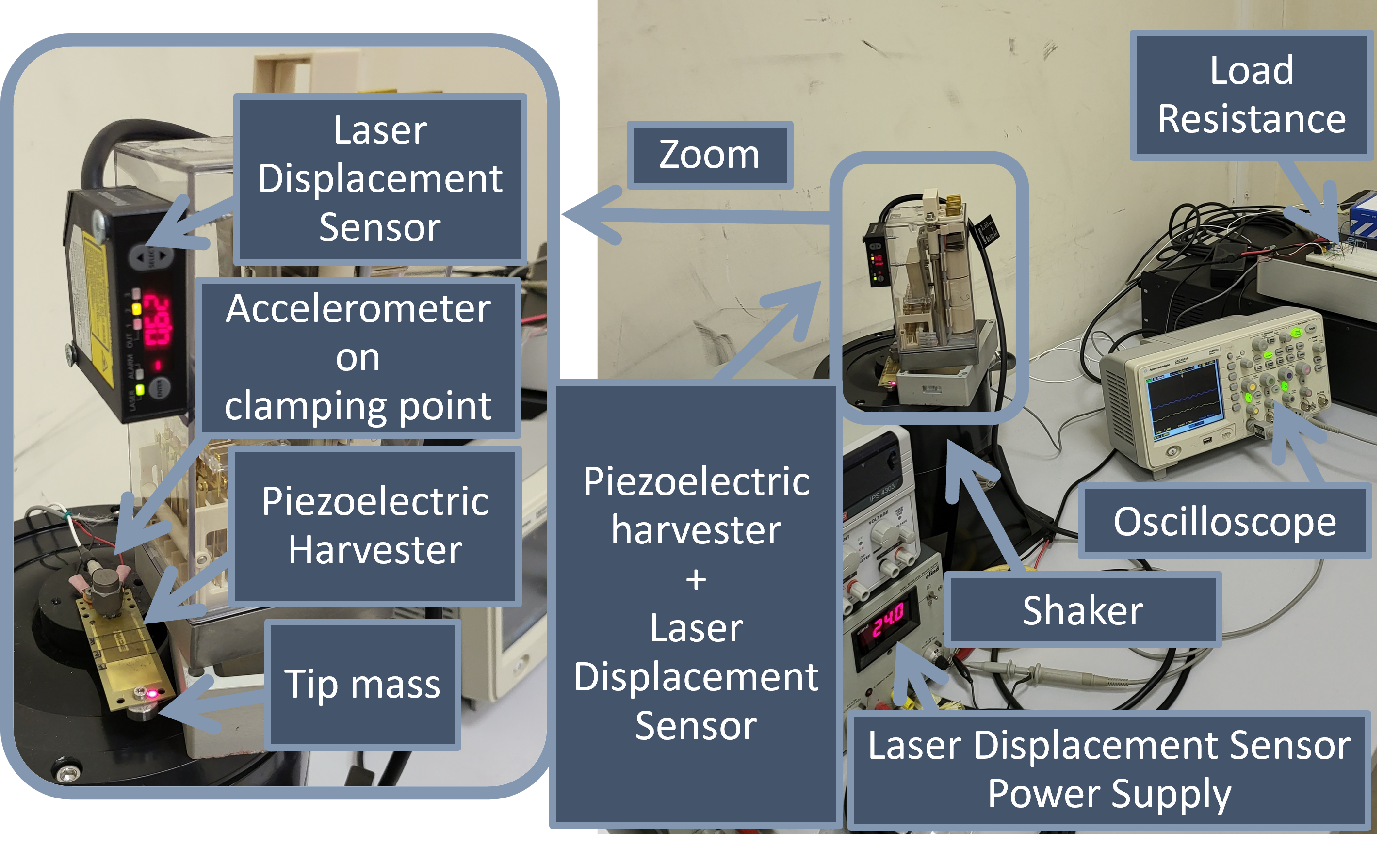
Figure 1: Picture of the experimental apparatus.

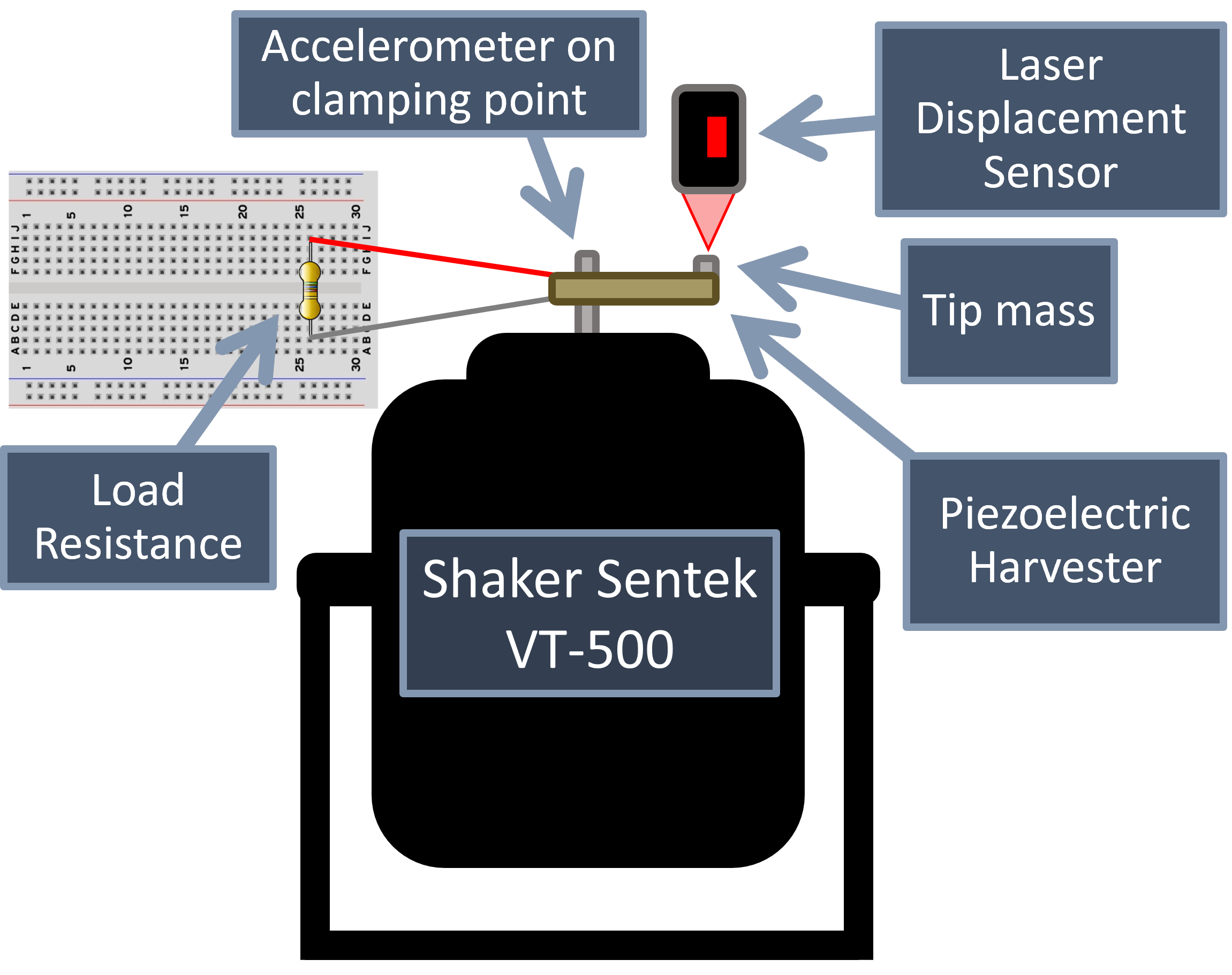
Figure 2: Schematic representation of a cantilever structure with piezoelectric energy harvester.

To study the response of the system to broadband vibrations, we fed the shaker with a Gaussian signal generated with standard software (MATLAB, R2023b) with a sampling rate $f=5$ kHz. From the measurement of the voltage $v_{p}$, we obtain the average extracted power $P_{harv}=\langle v_{p}^{2}\rangle/R$, where $R$ is the load resistance and $\langle\ldots\rangle$ denotes an average in the stationary state. The study of the system for different vibration amplitudes and for a wide range of load resistances is reported in Costanzo et al. (2021).

III Theoretical Model

The piezoelectric energy harvester introduced in the previous section can be accurately described with the following linear model Costanzo et al. (2021):

$$\begin{cases}\dot{x}=v,\\ M\dot{v}=-K_{s}x-\gamma v-\theta v_{p}+M\xi,\\ C_{p}\dot{v}_{p}=\theta v-\frac{v_{p}}{R},\end{cases}$$ (1)

where $\xi$ is white noise with zero mean and correlation $\langle\xi(t)\xi(t^{\prime})\rangle=2D_{0}\delta(t-t^{\prime})$. In the above equations, $x$ represents the displacement of the effective tip mass $M$ along the vertical direction, $v$ its velocity, $\gamma$ the viscous damping due to the air friction, $K_{s}$ the stiffness of the cantilever in the harmonic approximation, $v_{p}$ the voltage across the load resistance $R$, $C_{p}$ the effective output capacitance of the piezoelectric transducer, and $\theta$ its effective electromechanical coupling factor.

As already observed in Costanzo et al. (2021), the system of equations can be rewritten as a non-Markovian model, where a memory is present in the dynamics. In particular, one has

$$\dot{v}=-\int_{0}^{t}\left[2\frac{\gamma}{M}\delta(t^{\prime})+\Gamma(t-t^{\prime})\right]v(t^{\prime})dt^{\prime}-\frac{K_{s}}{M}x+\xi,$$ (2)

where the memory kernel $\Gamma(t)$ has the exponential form

$$\Gamma(t)=\frac{\theta^{2}}{C_{p}M}e^{-t/RC_{P}}.$$ (3)

From this formulation of the model, one can immediately observe that the friction memory kernel $\Gamma(t)$ is not associated with any noise term. This makes the system out of equilibrium, because the fluctuation–dissipation relation of the second kind is explicitly broken. Note that a noise term on the dynamical equation of the voltage could be also considered, due to the presence of thermal fluctuations in the circuit (Johnson noise). However, in this setup, such a term is negligible. In order to make it relevant, the  amplitude of the shaker should be significantly reduced.

Stationary Quantities

For the linear model introduced above the static properties can be easily obtained by standard methods Risken (1989). Introducing the column vector ${\bf X}=(x,v,v_{p})^{T}$ and the coupling matrix

$${\bf A}=\left(\begin{array}[]{ccc}0&-1&0\\ \frac{K_{s}}{M}&\frac{\gamma}{M}&\frac{\theta}{M}\\ 0&-\frac{\theta}{C_{p}}&\frac{1}{C_{p}R}\end{array}\right),$$ (4)

Equation (1) can be rewritten in vectorial form as

$$\dot{{\bf X}}=-{\bf A}{\bf X}+{\boldsymbol{\eta}},$$ (5)

where ${\boldsymbol{\eta}}=(0,\xi,0)^{T}$. Introducing the covariance matrix ${\boldsymbol{\sigma}}=\langle X^{T}X\rangle$ as

$${\boldsymbol{\sigma}}=\left(\begin{array}[]{ccc}\sigma_{xx}&\sigma_{xv}&\sigma_{xv_{p}}\\ \sigma_{vx}&\sigma_{vv}&\sigma_{vv_{p}}\\ \sigma_{v_{p}x}&\sigma_{v_{p}v}&\sigma_{v_{p}v_{p}}\end{array}\right),$$ (6)

at stationarity, one has the constraint

$${\boldsymbol{D}}=\frac{{\bf A}{\boldsymbol{\sigma}}+{\boldsymbol{\sigma}}{\bf A}^{T}}{2},$$ (7)

where ${\bf D}$ is the noise matrix

$${\bf D}=\left(\begin{array}[]{ccc}0&0&0\\ 0&D_{0}&0\\ 0&0&0\end{array}\right).$$ (8)

The stationary distribution is a multivariate Gaussian

$$P_{st}(x,v,v_{p})\sim e^{-\frac{1}{2}\left(\sigma_{xx}^{-1}x^{2}+\sigma_{vv}^{-1}v^{2}+\sigma_{v_{p}v_{p}}^{-1}v_{p}^{2}+2\sigma_{xv}^{-1}xv+2\sigma_{xv_{p}}^{-1}xv_{p}+2\sigma_{vv_{p}}^{-1}vv_{p}\right)},$$ (9)

where ${\boldsymbol{\sigma}}^{-1}$ denotes the inverse matrix of ${\boldsymbol{\sigma}}$. From this expression, we can obtain the marginalized probability distribution of the quantity $v_{p}$ as

$$P(v_{p})=\int_{-\infty}^{\infty}dx\int_{-\infty}^{\infty}dvP_{st}(x,v,v_{p})=\frac{1}{\sqrt{2\pi}\sigma_{v_{p}v_{p}}}e^{-\frac{v_{p}^{2}}{2\sigma^{2}_{v_{p}v_{p}}}},$$ (10)

where

$$\sigma_{v_{p}v_{p}}=\langle v_{p}^{2}\rangle=\frac{D_{0}\theta^{2}M^{2}R^{2}}{\gamma C_{p}R\left(\gamma+C_{p}K_{s}R+\theta^{2}R\right)+M\left(\gamma+\theta^{2}R\right)}.$$ (11)

The average output power is then given by

$$P_{harv}=\frac{1}{R}\langle v_{p}^{2}\rangle.$$ (12)

The linear model described by Equations (1) features physical parameters that can be directly controlled in the experiments and others whose values can be fitted to match the measured data. The amplitude of the white noise $D_{0}$ is related to the acceleration $a$ provided by the shaker and to the sampling rate $1/\Delta t$ of the input signal, $D_{0}=a^{2}\Delta t/2$, where $\Delta t=1/f=0.0002$ s. The mechanical parameters $K_{s}$ and $M$ are related to the characteristic frequency of the system, which for the experimental apparatus is $\sqrt{K_{s}/M}=2\pi\times 91$ Hz. Finally, the capacitor $C_{p}$ is estimated as $C_{p}\sim 490$ nF. The other parameters can be fitted to the experimental data through Equation (12) as a function of $R$. We performed several experiments with different values of $R\in[2700-3900]$ $\Omega$ and measured the average extracted power $P_{harv}$. From the fit, we obtain the following values: $M=0.0198\pm 0.005$ Kg, $\theta=0.00895\pm 0.0005$ N/V, $\gamma=0.3592\pm 0.005$ Kg/s. The shaker acceleration is $a=0.8\times 9.81$ m/s². Using these values of the parameters, we performed numerical simulations of the model in Equation (1) to measure the quantity $v_{p}(t)$ in the case $R=2700,3000,3900$ $\Omega$ and its distributions. The numerical results are in very good agreement with experimental data (see Figure 3), showing that the linear model very well describes the dynamics of the system. Once assessed the effectiveness of the theoretical model, we next focus on the study of the non-equilibrium properties of the system, as discussed in the following section.

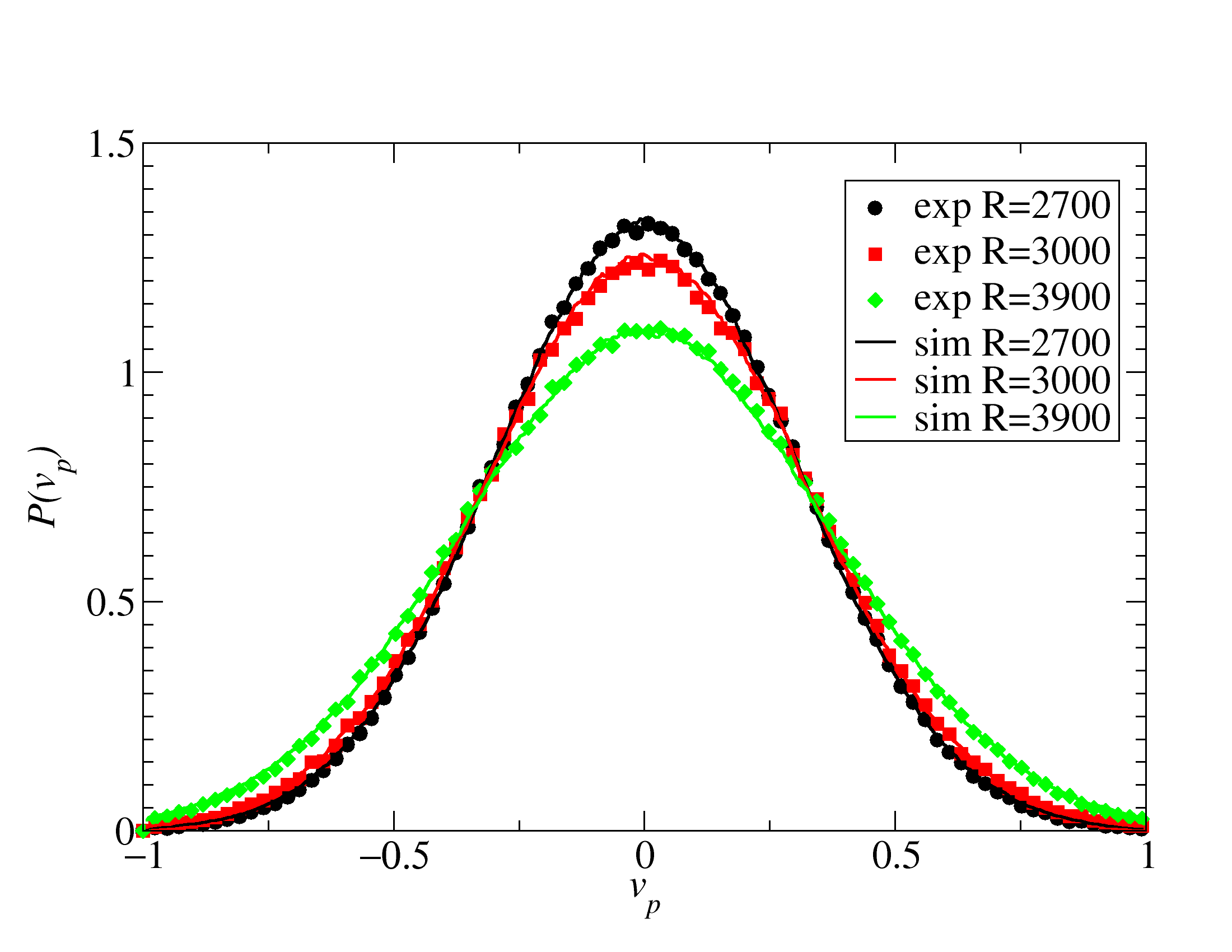
Figure 3: Comparison between the experimental data (symbols) and the theoretical model (lines). The probability distributions $P(v_{p})$ measured in experiments and in numerical simulations show a very good agreement, with the parameters reported in the main text and load resistances $R\in[2700,3900]$ $\Omega$.

IV Inference of Time-Reversal Asymmetry

The non-equilibrium nature of a system is reflected in the time-reversal asymmetry of the dynamics, which can manifest in different quantities and can be checked in several ways (see, for instance, the accurate discussion reported in Lucente et al. (2022) and the review Zanin and Papo (2021)). The more common quantity introduced to study the off-equilibrium character of a system is the fluctuating entropy production (EP), which can be defined at the level of a single trajectory of the dynamics, considering the ratio between the probability of observing a trajectory in the phase space and the probability of observing the time-reversed trajectory (obtained by visiting the same states in the phase space, but in reversed order) Lebowitz and Spohn (1999). This quantity strictly vanishes in equilibrium, where detailed balance holds, but is different from zero when energy currents are present and can be considered as a measure of how far the system departs from equilibrium. To measure such a quantity requires direct access to all degrees of freedom in the system that are responsible for non-equilibrium behaviors. In numerical simulations, this is generally possible, whereas in real experiments the task is usually much more difficult. Indeed, often, one can obtain only partial information on the system under study due to the limitation of the experimental apparatus that can measure some specific quantities. Therefore, in recent years, a lot of attempts have been made to provide estimations or bounds on EP from the measurement of currents directly accessible in experiments. This led to the development of the so-called thermodynamic uncertainty relations, opening a large field of research Barato and Seifert (2015); Roldán et al. (2021); Manikandan et al. (2020); Ghosal and Bisker (2022); Martínez et al. (2019); Uhl et al. (2018); Kim et al. (2022); Dechant et al. (2023); Dechant (2023).

Other approaches to assess non-equilibrium behaviors are based on the application of the fluctuation–dissipation relation. For systems in thermal equilibrium, this relation takes a very simple structure, relating the response of a quantity to an external perturbation with the fluctuations of the same quantity (namely the auto-correlation function) computed in the unperturbed dynamics, the  constant of proportionality between response and autocorrelation being the temperature. On the other hand, in non-equilibrium conditions, violations of this relation can be observed, revealing the off-equilibrium dynamics of the system. Kubo (1966); Ruelle (1998); Speck and Seifert (2006); Baiesi et al. (2009); Sarracino et al. (2010); Sarracino (2013); Gnoli et al. (2014); Puglisi et al. (2017). However, the study of the validity of the equilibrium relation requires performing response experiments. This means that a perturbation of the system, changing some external parameters, has to be introduced in order to measure the response function. This is not always simple in real experiments. Let us also mention that generalized Fluctuation-Dissipation Relations, valid also out of equilibrium have been derived Marconi et al. (2008), but these take a more complex structure and involve cross-correlations between different degrees of freedom.

Another interesting way to put in evidence the time-asymmetric character of the dynamics is based on the analysis of the shape of the avalanches reconstructed from the signal. An avalanche is defined as a region of the stochastic trajectory between two successive passages through a given threshold value. This analysis plays a central role in different physical systems, see for instance Blumenthal (2012); Majumdar and Orland (2015); Baldassarri (2021); de Candia et al. (2021), where asymmetric shapes of the avalanche profiles can be observed. The difficulty of such an analysis depends on the fact that a large amount of statistics is necessary to accurately reconstruct the avalanche profiles.

Here we will address the problem by exploiting a further approach, which focuses on the time-reversal properties of higher-order correlation functions. This alternative way to reveal irreversible dynamics was first proposed in Pomeau (1982), and has been recently applied for granular systems in Lucente et al. (2023). See also Ref. Pomeau and Piasecki (2017) for an interesting discussion on correlations in the Langevin equation. In general, it can be shown that a system is at equilibrium if the correlation $C_{fg}(t)\equiv\langle f(t)g(0)\rangle=\langle g(t)f(0)\rangle=C_{gf}(t)$, for all functions $f$ and $g$. For stationary systems, this is equivalent to the condition $C_{fg}(t)=C_{fg}(-t)$. However, when the system is linear, the time-reversal asymmetry cannot be revealed by the study of a single observable, and cross-correlations have to be taken into account. The main aim of this work is to provide an explicit example of this problem with the analysis of experimental data, as discussed in the following.

IV.1 Data Analysis

We address the issue related to the (non-)equilibrium nature of the system and its time-reversal symmetries analyzing time series of two measured quantities: $v_{p}(t)$, the voltage at the resistance load, and $v_{z}(t)$, the voltage at the displacement sensor, related to the tip mass dynamics. We first show in Figure 4 the normalized temporal autocorrelation functions of $v_{p}(t)$ and $v_{z}(t)$,

$$C_{v_{p}}(t) \equiv \frac{\langle v_{p}(t)v_{p}(0)\rangle}{\langle v_{p}(0)v_{p}(0)\rangle},$$ (13)

$$C_{v_{z}}(t) \equiv \frac{\langle v_{z}(t)v_{z}(0)\rangle}{\langle v_{z}(0)v_{z}(0)\rangle},$$ (14)

that are characterized by an exponential decay, modulated by an oscillatory behavior. The characteristic decay time is estimated as $\tau_{exp}\simeq 0.118\pm 0.005$ s, while the oscillation period is $T_{exp}\simeq 0.010\pm 0.005$ s. These values are in good agreement with the theoretical values obtained from the study of the eigenvalues of the matrix ${\bf A}$ of the model, which give $\tau=0.079$ s and $T=0.0109$ s. An accurate study of the analytical form of time correlation functions in non-Markovian systems is presented in Doerries et al. (2021).

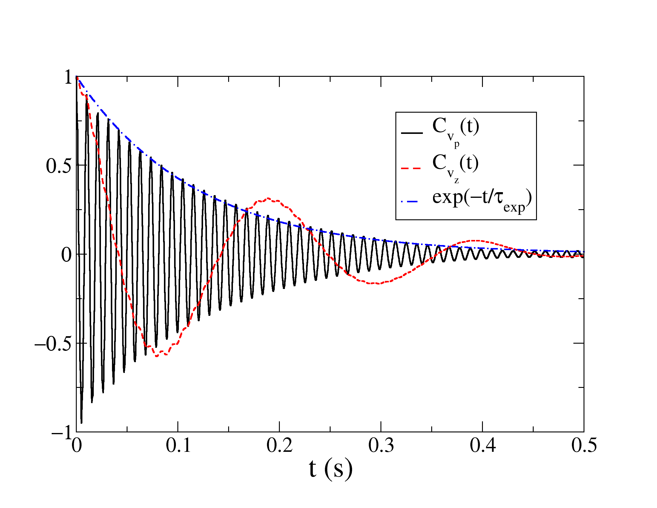
Figure 4: Temporal autocorrelation functions of $v_{p}(t)$ and $v_{z}(t)$ measured in experiments.

By construction, from these two-point autocorrelation functions, one cannot extract any information on the irreversible dynamics of the system. In order to define correlation functions with a single variable that could unveil a time-asymmetry, one has to consider higher-order correlators. In particular, from the time series of $v_{p}(t)$ and $v_{z}(t)$, we compute the following normalized correlation functions:

$$C^{(4)}_{v_{p}}(t) \equiv \frac{\langle v_{p}(t)v^{3}_{p}(0)\rangle}{\langle v^{4}_{p}(0)\rangle},$$ (15)

$$C^{(4)}_{v_{z}}(t) \equiv \frac{\langle v_{z}(t)v^{3}_{z}(0)\rangle}{\langle v^{4}_{z}(0)\rangle},$$ (16)

We note that, since the averages $\langle v_{z}(t)\rangle=\langle v_{p}(t)\rangle=0$, the total order of the correlation must be even (otherwise the normalization at zero time would be zero), and therefore, we consider the correlation between a variable and its third power.

For a linear system, it has been shown Lucente et al. (2022) that from the observation of a single quantity, one cannot obtain information on the non-equilibrium nature of the system. This is due to the fact that linear systems present Gaussian statistics. Therefore, a multi-point correlator can be expressed in terms of two-point correlation functions, which are always symmetric under time-reversal by construction. Our experimental data illustrate this mechanism. Indeed, as reported in Figure 5, from the analysis of a single observable, even considering higher order correlation functions, time-reversal symmetry cannot be observed. This is clear from the behavior of the functions $C^{(4)}_{v_{p}}(t)-C^{(4)}_{v_{p}}(-t)$ and $C^{(4)}_{v_{z}}(t)-C^{(4)}_{v_{z}}(-t)$, which vanish in both cases. This result further corroborates the efficacy of the linear model Equations (1) to describe the experimental setup: indeed, the presence of some relevant nonlinearities in the system could make the correlation functions $C^{(4)}_{v_{p}}(t)$ and $C^{(4)}_{v_{p}}(-t)$ different due to the out-of-equilibrium nature of the system.

On the other hand, the time-reversal asymmetry in the model can be clearly revealed if one considers the cross-correlation between the two coupled variables $v_{p}(t)$ and $v_{z}(t)$

$$C_{v_{p}v_{z}}(t) \equiv \frac{\langle v_{p}(t)v_{z}(0)\rangle}{\langle v_{p}(0)v_{z}(0)\rangle},$$ (18)

$$C_{v_{z}v_{p}}(t) \equiv \frac{\langle v_{z}(t)v_{p}(0)\rangle}{\langle v_{p}(0)v_{z}(0)\rangle}=C_{v_{p}v_{z}}(-t),$$ (19)

as shown in Figure 6.

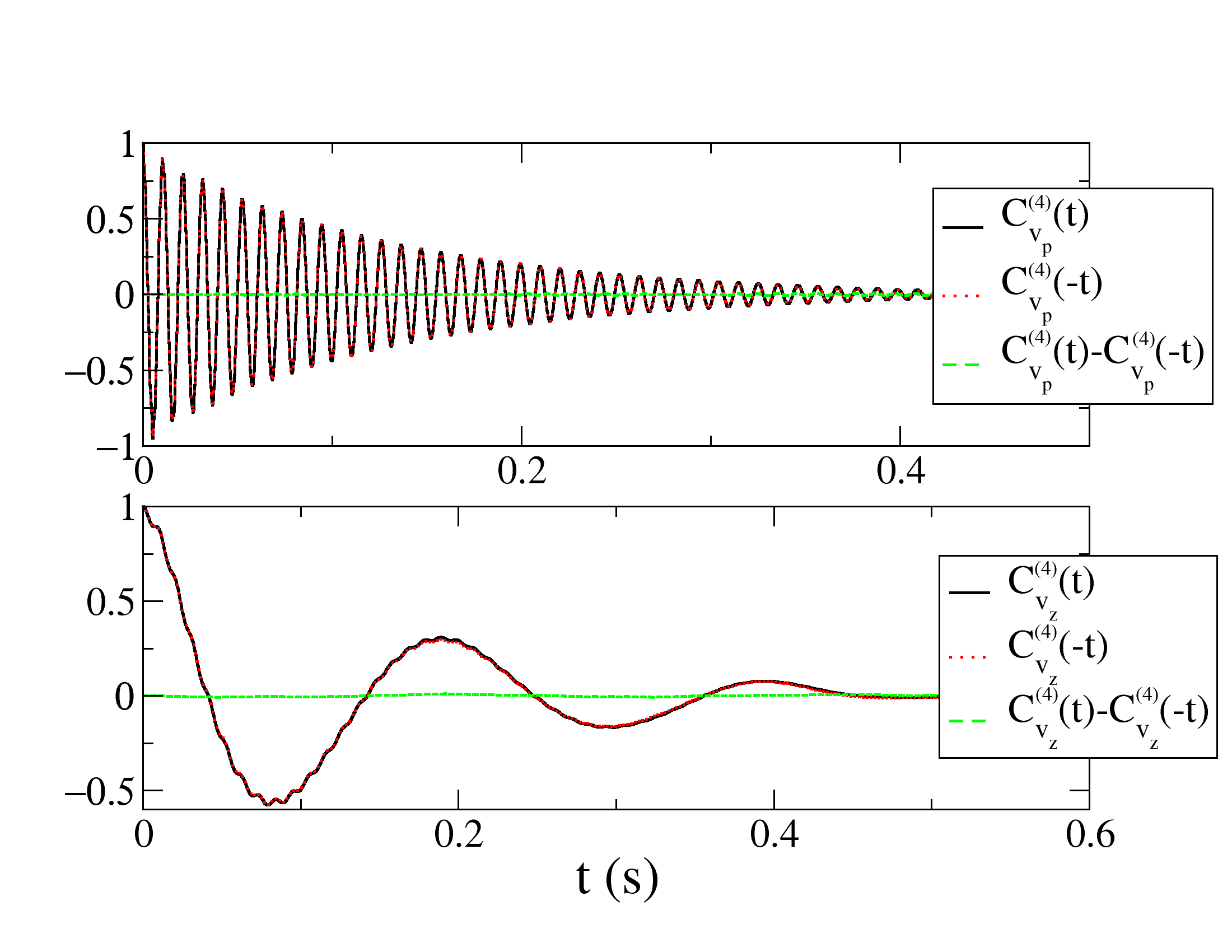
Figure 5: High-order correlation functions $C^{(4)}_{v_{p}}(t)$ and $C^{(4)}_{v_{z}}(t)$ obtained from real data measured in experiments. We note that from the analysis of a single variable the dynamics appears symmetric under time-reversal, as evidenced by $C^{(4)}_{v_{z}}(t)-C^{(4)}_{v_{z}}(-t)$, which is zero at all times.

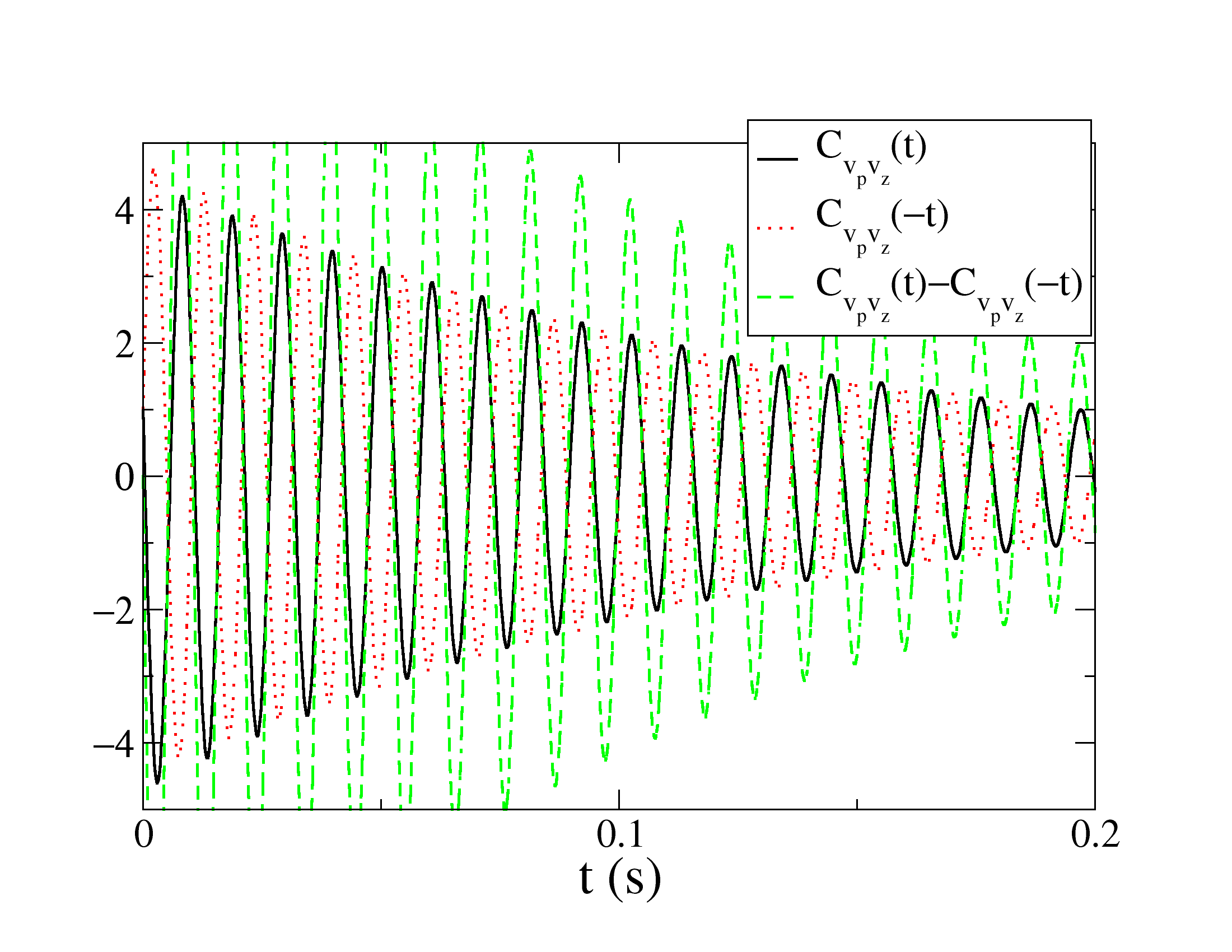
Figure 6: Cross-correlation function $C_{v_{p}v_{z}}(t)$ obtained from real data measured in experiments. The non-equilibrium time-asymmetric dynamics of the system clearly appears from the observation of the coupled motion of $v_{p}$ and $v_{z}$, as evidenced by $C_{v_{p}v_{z}}(t)-C_{v_{p}v_{z}}(-t)$, which differs from zero.

IV.2 Numerical Simulations

To further support our findings, we performed the same analysis on the numerical simulations of the model Equation (1). In particular, we numerically computed the voltage $v_{p}(t)$, the velocity $v(t)$, and the position $x(t)$, which can be directly accessed in the simulations. The results reported in Figure 7 confirm the scenario described above for the experimental data: analyses of (high-order) correlations of a single variable do not allow one to reveal a non-equilibrium behavior (top and bottom panels), whereas cross-correlation functions show the breaking of the time-reversal symmetry (middle panel).

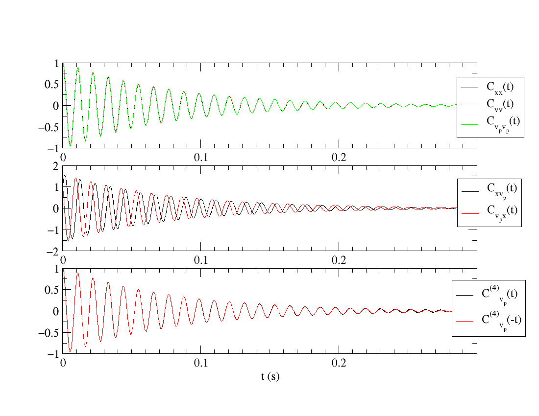
Figure 7: Correlation functions obtained in numerical simulations (parameter values are the same as those fitted to the experimental data with $R=3000$ $\Omega$). In the top panel, the autocorrelations of position, velocity and load voltage are reported, showing all the same behavior. The cross correlations between $x$ and $v_{p}$ shown in the middle panel reveal the time-asymmetry of the dynamics. In the bottom panel, high-order correlations of $v_{p}$ are reported: both $C^{4}_{v_{p}}(t)$ and its time-reversed $C^{4}_{v_{p}}(-t)$ show the same behavior.

V Conclusions

We presented an experimental and theoretical study of a piezoelectric energy harvester driven by white noise vibrations, with the aim to illustrate the problem of extracting information on non-equilibrium dynamics of a system from real time series. We have first shown that the system can be well described by an effective linear model, featuring an inertial Brownian particle in a parabolic potential, coupled with an auxiliary variable. This second quantity describes the electromechanical coupling between the tip mass of the piezoelectric device with the electronic circuit. The total system is by construction out of equilibrium because the auxiliary variable is not in contact with any thermostat.

We then focused on the analysis of the temporal correlation functions of the measured quantities, load voltage $v_{p}(t)$ and displacement voltage $v_{z}(t)$, in order to illustrate the problem of assessing the non-equilibrium behavior of the system. As expected, from the observation of a single quantity, even for higher order correlations, the time-reversal asymmetry cannot be revealed due to the linearity of the model. However, when cross-correlations are considered, the non-equilibrium, time-asymmetric dynamics are unveiled. Numerical simulations of the theoretical model confirm the emerging scenario.

This work paves the way for other studies concerning non-equilibrium features, such as entropy production, in this kind of experimental system, where memory and feedback effects are present. For instance, the study of the entropy production can provide information on the distance from equilibrium of the system as a function of the model parameters. In particular, the relevance of fluctuations in our setup can be described via the introduction of the concept of effective temperature Puglisi et al. (2017), related to the amplitude vibration of the shaker. This approach is common in macroscopic athermal systems, such as vibro-fluidized granular fluids Gnoli et al. (2013), where the notion of effective temperature can be useful to try to extend the theoretical framework of statistical mechanics to non-equilibrium systems. In our case, a similar treatment could be attempted, and a definition of entropy production could be provided in terms of such an effective parameter. We plan to study this generalization in our model in future works.

References

References

- Brenes et al. (2020) Brenes, A.; Morel, A.; Juillard, J.; Lefeuvre, E.; Badel, A. Maximum power point of piezoelectric energy harvesters: A review of optimality condition for electrical tuning. Smart Mater. Struct. 2020, 29, 033001.
- Halvorsen (2008) Halvorsen, E. Energy harvesters driven by broadband random vibrations. J. Microelectromechanical Syst. 2008, 17, 1061.
- Costanzo et al. (2021) Costanzo, L.; Lo Schiavo, A.; Sarracino, A.; Vitelli, M. Stochastic thermodynamics of a piezoelectric energy harvester model. Entropy 2021, 23, 677.
- Reimann (2002) Reimann, P. Brownian motors: Noisy transport far from equilibrium. Phys. Rep. 2002, 361, 57.
- Zwanzig (2001) Zwanzig, R. Nonequilibrium Statistical Mechanics; Oxford University Press: Oxford, UK, 2001.
- Gnesotto et al. (2018) Gnesotto, F.S.; Mura, F.; Gladrow, J.; Broedersz, C.P. Broken detailed balance and non-equilibrium dynamics in living systems: A review. Rep. Prog. Phys. 2018, 81, 066601.
- Roldán et al. (2021) Roldán, É.; Barral, J.; Martin, P.; Parrondo, J.M.; Jülicher, F. Quantifying entropy production in active fluctuations of the hair-cell bundle from time irreversibility and uncertainty relations. New J. Phys. 2021, 23, 083013.
- Pigolotti and Vulpiani (2008) Pigolotti, S.; Vulpiani, A. Coarse graining of master equations with fast and slow states. J. Chem. Phys. 2008, 128, 154114.
- Puglisi et al. (2010) Puglisi, A.; Pigolotti, S.; Rondoni, L.; Vulpiani, A. Entropy production and coarse graining in Markov processes. J. Stat. Mech. Theory Exp. 2010, 2010, P05015.
- Teza and Stella (2020) Teza, G.; Stella, A.L. Exact coarse graining preserves entropy production out of equilibrium. Phys. Rev. Lett. 2020, 125, 110601.
- Seifert (2012) Seifert, U. Stochastic thermodynamics, fluctuation theorems and molecular machines. Rep. Prog. Phys. 2012, 75, 126001.
- Marconi et al. (2008) Marconi, U.M.B.; Puglisi, A.; Rondoni, L.; Vulpiani, A. Fluctuation-dissipation: Response theory in statistical physics. Phys. Rep. 2008, 461, 111.
- Puglisi et al. (2017) Puglisi, A.; Sarracino, A.; Vulpiani, A. Temperature in and out of equilibrium: A review of concepts, tools and attempts. Phys. Rep. 2017, 709, 1–60.
- Di Leonardo et al. (2010) Di Leonardo, R.; Angelani, L.; Dell’Arciprete, D.; Ruocco, G.; Iebba, V.; Schippa, S.; Conte, M.P.; Mecarini, F.; De Angelis, F.; Di Fabrizio, E. Bacterial ratchet motors. Proc. Natl. Acad. Sci. USA 2010, 107, 9541–9545. https://doi.org/10.1073/pnas.0910426107.
- Puglisi et al. (2018) Puglisi, A.; Sarracino, A.; Vulpiani, A. Thermodynamics and Statistical Mechanics of Small Systems. Entropy 2018, 20, 392.
- Cohen and Mauzerall (2004) Cohen, E.; Mauzerall, D. A note on the Jarzynski equality. J. Stat. Mech. Theory Exp. 2004, 2004, P07006.
- Gujrati (2020) Gujrati, P. Jensen inequality and the second law. Phys. Lett. A 2020, 384, 126460.
- Diks et al. (1995) Diks, C.; Van Houwelingen, J.; Takens, F.; DeGoede, J. Reversibility as a criterion for discriminating time series. Phys. Lett. A 1995, 201, 221–228.
- Crisanti et al. (2012) Crisanti, A.; Puglisi, A.; Villamaina, D. Nonequilibrium and information: The role of cross correlations. Phys. Rev. E 2012, 85, 061127.
- Lucente et al. (2022) Lucente, D.; Baldassarri, A.; Puglisi, A.; Vulpiani, A.; Viale, M. Inference of time irreversibility from incomplete information: Linear systems and its pitfalls. Phys. Rev. Res. 2022, 4, 043103.
- Lucente et al. (2023) Lucente, D.; Viale, M.; Gnoli, A.; Puglisi, A.; Vulpiani, A. Out-of-Equilibrium Non-Gaussian Behavior in Driven Granular Gases. Phys. Rev. Lett. 2023, 131, 078201.
- Costanzo et al. (2022) Costanzo, L.; Lo Schiavo, A.; Sarracino, A.; Vitelli, M. Stochastic Thermodynamics of an Electromagnetic Energy Harvester. Entropy 2022, 24, 1222.
- Sagawa and Ueda (2012) Sagawa, T.; Ueda, M. Nonequilibrium thermodynamics of feedback control. Phys. Rev. E 2012, 85, 021104.
- Munakata and Rosinberg (2014) Munakata, T.; Rosinberg, M. Entropy production and fluctuation theorems for Langevin processes under continuous non-Markovian feedback control. Phys. Rev. Lett. 2014, 112, 180601.
- Munakata and Rosinberg (2013) Munakata, T.; Rosinberg, M. Feedback cooling, measurement errors, and entropy production. J. Stat. Mech. Theory Exp. 2013, 2013, P06014.
- Rosinberg et al. (2015) Rosinberg, M.; Munakata, T.; Tarjus, G. Stochastic thermodynamics of Langevin systems under time-delayed feedback control: Second-law-like inequalities. Phys. Rev. E 2015, 91, 042114.
- Doerries et al. (2021) Doerries, T.J.; Loos, S.A.; Klapp, S.H. Correlation functions of non-Markovian systems out of equilibrium: Analytical expressions beyond single-exponential memory. J. Stat. Mech. Theory Exp. 2021, 2021, 033202.
- Loos and Klapp (2019) Loos, S.A.; Klapp, S.H. Fokker–Planck equations for time-delayed systems via Markovian embedding. J. Stat. Phys. 2019, 177, 95–118.
- De Martino and Barato (2019) De Martino, D.; Barato, A.C. Oscillations in feedback-driven systems: Thermodynamics and noise. Phys. Rev. E 2019, 100, 062123.
- Debiossac et al. (2022) Debiossac, M.; Rosinberg, M.L.; Lutz, E.; Kiesel, N. Non-Markovian feedback control and acausality: An experimental study. Phys. Rev. Lett. 2022, 128, 200601.
- Plati et al. (2023) Plati, A.; Puglisi, A.; Sarracino, A. Thermodynamic bounds for diffusion in nonequilibrium systems with multiple timescales. Phys. Rev. E 2023, 107, 044132.
- Risken (1989) Risken, H. The Fokker-Planck Equation: Methods of Solution and Applications; Springer: Berlin, Germany, 1989.
- Zanin and Papo (2021) Zanin, M.; Papo, D. Algorithmic approaches for assessing irreversibility in time series: Review and comparison. Entropy 2021, 23, 1474.
- Lebowitz and Spohn (1999) Lebowitz, J.L.; Spohn, H. A Gallavotti-Cohen-Type Symmetry in the Large Deviation Functional for Stochastic Dynamics. J. Stat. Phys. 1999, 95, 333.
- Barato and Seifert (2015) Barato, A.C.; Seifert, U. Thermodynamic Uncertainty Relation for Biomolecular Processes. Phys. Rev. Lett. 2015, 114, 158101. https://doi.org/10.1103/PhysRevLett.114.158101.
- Manikandan et al. (2020) Manikandan, S.K.; Gupta, D.; Krishnamurthy, S. Inferring entropy production from short experiments. Phys. Rev. Lett. 2020, 124, 120603.
- Ghosal and Bisker (2022) Ghosal, A.; Bisker, G. Inferring entropy production rate from partially observed Langevin dynamics under coarse-graining. Phys. Chem. Chem. Phys. 2022, 24, 24021–24031.
- Martínez et al. (2019) Martínez, I.A.; Bisker, G.; Horowitz, J.M.; Parrondo, J.M. Inferring broken detailed balance in the absence of observable currents. Nat. Commun. 2019, 10, 3542.
- Uhl et al. (2018) Uhl, M.; Pietzonka, P.; Seifert, U. Fluctuations of apparent entropy production in networks with hidden slow degrees of freedom. J. Stat. Mech. Theory Exp. 2018, 2018, 023203.
- Kim et al. (2022) Kim, D.K.; Lee, S.; Jeong, H. Estimating entropy production with odd-parity state variables via machine learning. Phys. Rev. Res. 2022, 4, 023051.
- Dechant et al. (2023) Dechant, A.; Garnier-Brun, J.; Sasa, S.I. Thermodynamic bounds on correlation times. arXiv 2023, arXiv:2303.13038.
- Dechant (2023) Dechant, A. Thermodynamic constraints on the power spectral density in and out of equilibrium. arXiv 2023, arXiv:2306.00417.
- Kubo (1966) Kubo, R. The fluctuation-dissipation theorem. Rep. Prog. Phys. 1966, 29, 255.
- Ruelle (1998) Ruelle, D. General linear response formula in statistical mechanics, and the fluctuation-dissipation theorem far from equilibrium. Phys. Lett. A 1998, 245, 220.
- Speck and Seifert (2006) Speck, T.; Seifert, U. Restoring a fluctuation-dissipation theorem in a nonequilibrium steady state. Europhys. Lett. 2006, 74, 391.
- Baiesi et al. (2009) Baiesi, M.; Maes, C.; Wynants, B. Fluctuations and Response of Nonequilibrium States. Phys. Rev. Lett. 2009, 103, 010602.
- Sarracino et al. (2010) Sarracino, A.; Villamaina, D.; Gradenigo, G.; Puglisi, A. Irreversible dynamics of a massive intruder in dense granular fluids. Europhys. Lett. 2010, 92, 34001.
- Sarracino (2013) Sarracino, A. Time asymmetry of the Kramers equation with nonlinear friction: Fluctuation-dissipation relation and ratchet effect. Phys. Rev. E 2013, 88, 052124.
- Gnoli et al. (2014) Gnoli, A.; Puglisi, A.; Sarracino, A.; Vulpiani, A. Nonequilibrium Brownian Motion beyond the Effective Temperature. PLoS ONE 2014, 9, e93720.
- Blumenthal (2012) Blumenthal, R.M. Excursions of Markov Processes; Springer Science & Business Media: Berlin/Heidelberg, Germany, 2012.
- Majumdar and Orland (2015) Majumdar, S.N.; Orland, H. Effective Langevin equations for constrained stochastic processes. J. Stat. Mech. Theory Exp. 2015, 2015, P06039.
- Baldassarri (2021) Baldassarri, A. Universal excursion and bridge shapes in abbm/cir/bessel processes. J. Stat. Mech. Theory Exp. 2021, 2021, 083211.
- de Candia et al. (2021) de Candia, A.; Sarracino, A.; Apicella, I.; de Arcangelis, L. Critical behaviour of the stochastic Wilson-Cowan model. PLoS Comput. Biol. 2021, 17, e1008884.
- Pomeau (1982) Pomeau, Y. Symétrie des fluctuations dans le renversement du temps. J. De Phys. 1982, 43, 859–867.
- Pomeau and Piasecki (2017) Pomeau, Y.; Piasecki, J. The Langevin equation. Comptes Rendus Phys. 2017, 18, 570–582.
- Gnoli et al. (2013) Gnoli, A.; Petri, A.; Dalton, F.; Gradenigo, G.; Pontuale, G.; Sarracino, A.; Puglisi, A. Brownian Ratchet in a Thermal Bath Driven by Coulomb Friction. Phys. Rev. Lett. 2013, 110, 120601.