Inverse nonlinearity compensation of hyperelastic deformation in dielectric elastomers for acoustic actuation

Abstract

This paper delves into the analysis of nonlinear deformation induced by dielectric actuation in pre-stressed ideal dielectric elastomers. It formulates a nonlinear ordinary differential equation governing this deformation based on the hyperelastic model under dielectric stress. Through numerical integration and neural network approximations, the relationship between voltage and stretch is established. Neural networks are employed to approximate solutions for voltage-to-stretch and stretch-to-voltage transformations obtained via an explicit Runge-Kutta method. The effectiveness of these approximations is demonstrated by leveraging them for compensating nonlinearity through the waveshaping of the input signal. The comparative analysis highlights the superior accuracy of the approximated solutions over baseline methods, resulting in minimized harmonic distortions when utilizing dielectric elastomers as acoustic actuators. This study underscores the efficacy of the proposed approach in mitigating nonlinearities and enhancing the performance of dielectric elastomers in acoustic actuation applications.

[1] organization=Department of Intelligence and Information, Seoul National University, city=Seoul, postcode=08826, country=Republic of Korea [2] organization=Department of Materials Science and Engineering, Seoul National University, city=Seoul, postcode=08826, country=Republic of Korea [3] organization=Research Institute of Advanced Materials (RIAM), Seoul National University, city=Seoul, postcode=08826, country=Republic of Korea [4] organization=Interdisciplinary Program in Artificial Intelligence (IPAI), Seoul National University, city=Seoul, postcode=08826, country=Republic of Korea [5] organization=Artificial Intelligence Institute (AII), Seoul National University, city=Seoul, postcode=08826, country=Republic of Korea

1 Introduction

Dielectric elastomers represent a distinct class of materials renowned for their exceptional response to electrical stimuli, manifesting substantial deformations upon activation. These elastomers, comprising compliant layers interspersed between electrodes [1], akin to rubber in their compliance, exhibit remarkable deformability when subjected to an electric field. The resultant electrostatic force-induced deformation enables the conversion of electrical energy into mechanical motion [1, 2]. Composed primarily of compliant elastomeric substances, these materials have garnered significant interest across diverse technological domains, laying the foundation for Dielectric Elastomer Actuators (DEAs).

DEAs, crafted with one or more layers of dielectric elastomeric material sandwiched between compliant electrodes, serve as transducers converting electrical energy into mechanical motion [1]. Voltage application across the electrodes induces charge accumulation, leading to elastomer layer deformation. Electrode materials encompass graphite powder, silicone oil, or graphite mixtures, ensuring compliance without constraining elastomer elongation [3]. These deformations propel the actuator, generating motion or force, albeit necessitating a high threshold voltage for effective transduction [2]. Proper treatments facilitate robust and tunable actuation with improved stretch response rates [4].

Initially recognized for remarkable areal expansion in the early 2000s [5], DEAs continue to evolve [6, 4] along with evolutions in the materials as mechanical actuators [7, 8, 9]. While boasting inherent stretchability, DEAs offer simplicity, cost-effectiveness, lightweight design, and versatile utility [10]. Their applications span diverse fields, including loudspeakers [11, 12, 13], soft robotics [14, 15], artificial muscles [16], vibration control [17], membrane resonators [18], noise cancellation, [19, 20] and adaptive sound filters [21]. The capability to produce substantial deformations and forces while maintaining a lightweight and relatively simple fabrication process underscores their engineering significance. Recent research efforts have focused on quantifying nonlinear dynamics and precise control of DEAs [22, 7].

Employing DEA as an acoustic actuator demands meticulous treatment due to human auditory sensitivity to even minor nonlinear distortions [23], whereas DEA introduces significant nonlinear distortions during voltage-induced elastic deformation [12]. These challenges stem not only from nonlinear elastic deformation [24, 25] but also from the nonlinear relationship between voltage and Maxwell stress, even within linear elastic models [26, 12]. Addressing these challenges necessitates controlling nonlinear deformation, akin to endeavors focused on enhancing the response characteristics of acoustic actuators [27, 28].

The dielectric elastomer’s deformation exhibits visco-hyperelastic behavior [8, 7]. Accurate models accounting for large strains and visco-hyperelasticity are imperative for such actuators. Goulbourne et al. [29] proposes an analytic solution for dielectric elastomer stretch during actuation, employing Maxwell-Faraday electrostatics and nonlinear elasticity. While adopting Ogden [30] and Mooney-Rivlin [31, 32] nonlinear models as approximations to elastic deformation, their solution closely mirrors the DEA model, yet there are potential for enhancement by incorporating more recent elastic models like neo-Hookean [24, 33] or Gent [25] nonlinear elasticity models.

Modeling viscous behavior necessitates time-varying solutions [34, 35, 36]. While this paper primarily focuses on time-invariant cases, notable analyses delve into dynamics, including mechanical properties dependent on temperature or pre-stress variations [37, 38]. Analyzing the acoustic properties of DEA requires the control of these different variables [39]. Recent approaches utilize neural networks to approximate time-dependent DEA dynamics, leveraging recurrent neural networks [40, 41] or reinforcement learning [42]. Irrespective of the dynamics involved, these methodologies aim to model the actuation system, commonly manifested through ordinary or partial differential equations (ODEs/PDEs).

Numerous methods exist for solving differential equations. Recent research has prominently explored employing neural networks (NNs) to approximate solutions. In the context of function approximation, neural networks have long been recognized as universal approximators [43, 44, 45]. Additionally, NNs have proven successful in approximating solutions to differential equations [46]. NNs are not limited to solving ODEs alone [46, 47]; they are applied extensively to tackle PDEs, including the Korteweg-de Vries (KdV) equation [48, 49, 50], or Navier-Stokes equations [51, 52, 48, 49]. They often leverage NNs to approximate the solutions [49, 48] or leverage explicitly differentiable implementations of the solvers [47, 53].

This paper delves into the problem of compensating for the nonlinear deformation caused by dielectric actuation. We deduce a nonlinear ODE using the hyperelastic energy inherent in an ideal DE-based system (section 4). Subsequently, we establish the relationship between voltage and stretch using both numerical integration methods and neural network approximations (section 5). Leveraging the approximated solution, we apply it to compensate for the nonlinear dielectric elastomer actuation. Our evaluation in section 6 demonstrates the effectiveness of these methods.

Figure 1: Overview of the system.

2 Related Works

2.1 Modeling Hyperelastic Deformation

The complex behavior of elastomers necessitates the use of hyperelastic theories to derive the elastic energy of DE-based systems [54]. Multiple models elucidate hyperelasticity, such as the neo-Hookean [33, 24], Gent [25], Mooney-Rivlin [31, 32], Ogden [30], and Arruda-Boyce [55]. Recent studies have been dedicated to understanding the behaviors of DEAs. For instance, Jia et al. [56], Li et al. [18] conducts an analytical study on a flat DE membrane’s in-plane deformation, while Zhu et al. [57], Garnell et al. [58] explores the nonlinear dynamics of a balloon-shaped DE, revealing (sub-)harmonic responses under specific actuation conditions. This paper is distinguished by the fact that unlike the former [56, 18], it analyzes an idealized DEA that does not consider viscous effects, and unlike the latter [57, 58], it analyzes a planar-shaped membrane. Additionally, this study aligns with literature analyzing the hyperelasticity using neo-Hookean model [38, 34, 59, 37, 60, 61, 62], which is adopted within strains without reaching limiting stretch [33, 25].

2.2 Inverse Nonlinearity Compensation

Leveraging the insights from modeling hyperelastic deformation, our objective is to develop compensation techniques that reverse the nonlinear forward model. In the context of control theory, similar problems have been tackled through inverse dynamics compensation (IDC) [63]. IDC involves calculating and applying controls to counteract disturbances or achieve precise movements in dynamic systems, frequently employed in robotics or biomechanics. For instance, Zou and Gu [64, 65] successfully applied IDC to manage viscous hysteresis in DEAs using experimentally measured data. Analogous to IDC, this paper focuses on processing input signals to nonlinear DEAs to attain linear actuation. We frame this as an inverse nonlinearity compensation (INC) problem aimed at controlling hyperelastic deformation induced by the Maxwell stress [66, 67]. Considering the function’s nonlinear and time-invariant nature, we categorize this inverse nonlinearity compensation process as a form of waveshaping.

2.3 Neural Waveshaping Functions

It is pertinent to acknowledge the conventional notion of waveshaping as a synthesis method [68], designed to generate timbres from sinusoidal inputs using a memoryless, shift-invariant nonlinear shaping function [69, 70]. This function introduces harmonic components to the input signal [71]. Recently, Hayes et al. [72] proposes a neural waveshaping unit (NEWT) that enhances a harmonic-plus-noise synthesizer [73] with neural networks, akin to differentiable digital signal processing (DDSP) [74]. NEWT employs multi-layer perceptions (MLPs) to learn continuous representations of waveshaping functions and performs comparably to DDSP in synthesis tasks, doing so more efficiently. Our method shares the same methodology as NEWT by implicitly learning the waveshaping function using a neural network. However, it’s crucial to highlight that we’re not engaged in a synthesis task. Specifically, the purpose of the waveshaping function in our context is diametrically opposite to conventional waveshaping; it aims to eliminate the harmonics rather than induce them. This distinction will be rigorously addressed in the subsequent section.

3 Problem Statement

Denote the stretch in DEA as $\lambda$. This is determined by both pre-stretch and electromagnetic deformations influenced by the amplified high voltage signal ${V}=\alpha\cdot{x}$. In this paper, equi-biaxial deformation, as depicted in Figure 2, is considered and the pre-stretch is applied in the same direction. This study focuses on two main aspects: modeling the system and controlling it. First, we construct a model of the voltage-stretch system using an ODE. By solving this ODE, we obtain a solution that relates voltage to stretch.

$$f: \ \mathbb{R}\to\mathbb{R},$$ (1)

$$\ {V}\mapsto\lambda$$ (2)

Subsequently, we aim to find a signal-mapping function:

$$g: \ \mathbb{R}\to\mathbb{R},$$ (3)

$$\ {x}\mapsto\hat{{x}},$$ (4)

such that the resulting DEA stretch $\hat{\lambda}=f(\alpha\cdot\hat{{x}})$ maintains a linear correlation with the original signal ${x}$. Function $g$ serves as an inverse nonlinearity compensator of $f$ if for some $a_{0},a_{1}\in\mathbb{R}$ with $a_{1}\neq 0$,

$$f(\alpha\cdot g({x}))=a_{0}+a_{1}{x}.$$ (5)

Upon determining the fixed $f$ and its corresponding compensator $g$, this paper proposes approximated solutions $f_{\theta}$ and $g_{\theta}$, parameterized by $\theta$, optimized to:

minimize $$\quad\|f_{\theta}({V})-f({V})\|+\|g_{\theta}({x})-g({x})\|,$$ (6)

subject to $$\quad{x}>0\quad\text{and}\quad{V}=\alpha{x}>0.$$ (7)

The subsequent sections delve into the problem statement. However, for a more structured approach, we initially derive the ODE model, propose an approximation method for its solutions $f$ and $f^{-1}$, and then demonstrate that the approximation alone satisfactorily addresses problem (6).

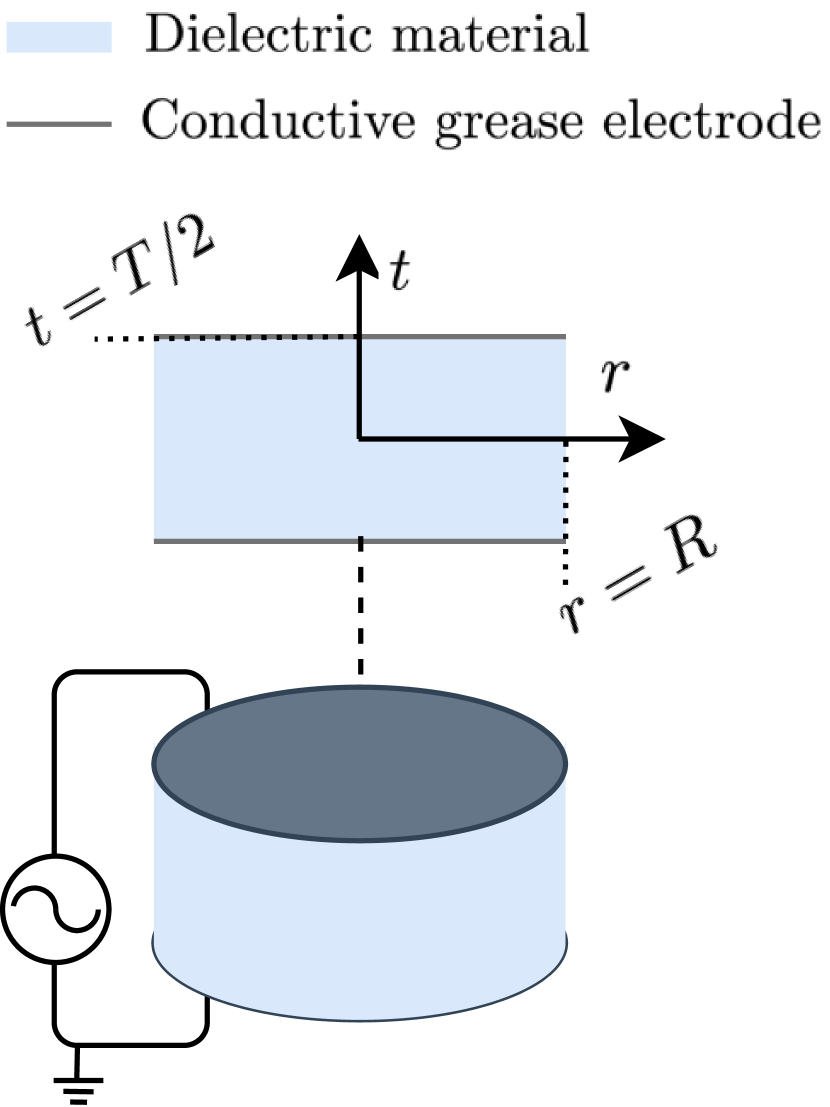
(a) Reference state

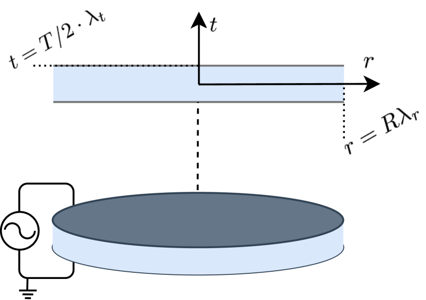
(b) Deformed state

Figure 2: Schematic diagram of dielectric system cross-section. (a) Reference state where no external force is applied. (b) Deformed state with equi-biaxial tension.

4 Simulating Dielectric Elastomer Actuator

Our focus initiates with the modeling of the voltage-stretch system, specifically delving into the electromechanical actuation of DEAs. We begin by defining the Helmholtz free energy of the elastomer as $A$. The potential energy $U$ of the dielectric elastomer is structured as per the formulations in [75, 76]:

$$U=A-W_{V}-W_{F}$$ (8)

Here, $A$ denotes the Helmholtz free energy, while $W_{V}$ represents the work done by the voltage, and $W_{F}$ depicts the work done by the tensile force. Applying the difference operator to equation (8) yields:

$$\delta A={V}\delta Q+F_{r}\delta\lambda_{r}$$ (9)

Defining the nominal density of the free energy as $W=A/(\pi R^{2}T)$, equation (9) can be reformulated as:

$$\pi R^{2}T\delta W={V}\delta Q+F_{r}\delta\lambda_{r}.$$ (10)

To further progress and derive an ODE for ${V}$ and $\lambda$, we express $\delta W$ and $\delta Q$ of equation (10) in terms of $\delta\lambda$. Before proceeding, we introduce specific assumptions in the actuation process to streamline the derivation of the equation of motion.

Assumption 1 (No polarization).

There exists no polarization between the electrodes. Hence, the electric displacement field is defined as $D=\varepsilon E$, where $\varepsilon$ and $E$ represent the dielectric constant and the electric field, respectively.

Assumption 2 (Incompressibility).

The dielectric elastomer is considered incompressible, signified by $J=\lambda_{r}\lambda_{\theta}\lambda_{t}=1$. Here, subscripts $r$, $\theta$, and $t$ refer to directions in cylindrical coordinates for radius, angle, and thickness.

Assumption 3 (No buckling).

The stretch along the angular direction $\lambda_{\theta}$ remains constant at a value of $1$ for all $\theta$, ensuring the absence of buckling in the dielectric elastomers.

Additionally, a free boundary condition is assumed, without support or clamping, and the electrode’s mass is considered negligibly small.

4.1 Electric Displacement

To reformulate $\delta Q$ in equation (10), we initially establish the relationship between the electric displacement and the electric field as per Assumption 1. Given the definitions of the electric field $E={V}/t$ and the electric displacement field $D=Q/(\pi r^{2})$, we derive:

$$\frac{Q}{\pi r^{2}}=\varepsilon\frac{{V}}{t}$$ (11)

Here, $r$ and $t$ represent the radius and thickness of the dielectric material in a deformed state, respectively. $\varepsilon=\varepsilon_{0}\varepsilon_{r}$ denotes the permittivity, where $\varepsilon_{0}$ signifies the vacuum permittivity, and $\varepsilon_{r}$ stands for the relative permittivity (or the dielectric constant). By rewriting $r=R\lambda_{r}$ and $t=T\lambda_{t}$, we arrive at the following expression:

$$Q=\varepsilon{V}\frac{\pi r^{2}}{t}=\varepsilon{V}\frac{\pi R^{2}}{T}\frac{\lambda_{r}^{2}}{\lambda_{t}}$$ (12)

Given Assumptions 2 and 3, where $\lambda_{r}\lambda_{t}=1$, equation (12) simplifies to:

$$Q={V}\frac{\pi R^{2}}{T}\frac{\varepsilon}{\lambda_{t}^{2}}.$$ (13)

Utilizing the difference operator $\delta\cdot$, we can express $\delta Q$ in terms of $\delta{V}$ and $\delta\lambda_{t}$:

$$\delta Q=\delta{V}\frac{\pi R^{2}}{T}\frac{\varepsilon}{\lambda_{t}^{2}}-2{V}\frac{\pi R^{2}}{T}\frac{\varepsilon}{\lambda_{t}^{3}}\cdot\delta\lambda_{t}$$ (14)

Substituting the $\delta Q$ using equation (14) further simplifies the equation (10).

4.2 Hyperelastic Deformation

To proceed, it remains to rephrase $\delta W$ in equation (10) in terms of $\delta\lambda_{t}$, integrating elastic deformation models into the analysis. Commencing with the free energy density originating from the neo-Hookean model [33, 24], it is represented as:

$$W=\frac{\mu}{2}(I-3)$$ (15)

Here, $I=\lambda_{r}^{2}+\lambda_{\theta}^{2}+\lambda_{t}^{2}$ characterizes the trace of the right Cauchy-Green deformation tensor. With Assumptions 2 and 3, the expression $I$ can be redefined as:

$$I=\lambda_{t}^{2}+1+\lambda_{t}^{-2}.$$ (16)

Consequently, the neo-Hookean free energy density in equation (15) transforms into:

$$W=\frac{\mu}{2}(\lambda_{t}^{2}+\lambda_{t}^{-2}-2)$$ (17)

Employing the difference operator allows us to express $\delta W$ of the neo-Hookean model using $\delta\lambda_{t}$:

$$\delta W=\mu(\lambda_{t}-\lambda_{t}^{-3})\delta\lambda_{t}$$ (18)

Finally, the reconfiguration of equation (10) using (14) and (18) results in the following ODE:

$$\frac{\delta{V}}{\delta\lambda_{t}}=2\frac{{V}}{\lambda_{t}}+\frac{\mu T^{2}}{\varepsilon{V}}(\lambda_{t}^{-1}-\lambda_{t}^{3})-\frac{F_{r}T}{\pi R^{2}}\cdot\frac{1}{\varepsilon{V}}$$ (19)

This equation encapsulates the relationship between the driving voltage and the stretch within the dielectric elastomer model, providing a foundation for further analysis.

Table 1: Mechanical properties

Notation	Value	Unit	Descriptions
$T$	$10^{-3}$	m	Initial thickness
$R$	$10^{-2}$	m	Initial radius
$Y$	$220$	kPa	Young’s modulus
$\varepsilon_{0}$	$8.85\times 10^{-12}$	$\text{C}^{2}/\text{m}^{2}\text{N}$	Vacuum permittivity
$\varepsilon_{r}$	$3.5$	-	Relative permittivity

5 Modeling the Voltage-Stretch Relation

To establish the relationship between voltage and stretch, it is crucial to solve the ODE (19). Solving (19) involves addressing this initial value problem (IVP) through the use of numerical integration techniques, as outlined in [77]. As the initial value, we set the reference state where $\lambda_{t}=1$ with $V=0$. We first introduce the numerical approximation that iteratively determines the solution starting from this initial value. Then, we present methods to estimate the solution obtained from the initial value problem without the need for integration calculations.

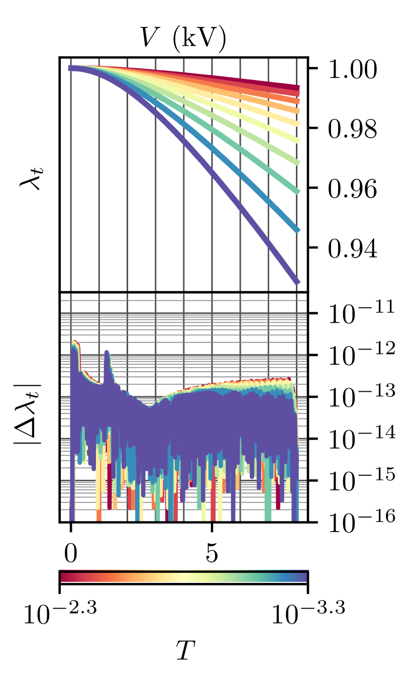
(a) Thickness $T$

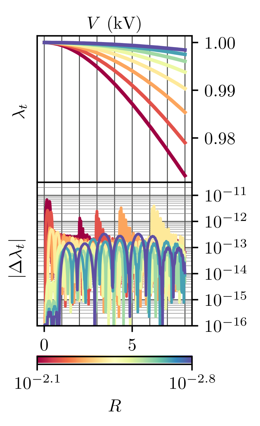
(b) Radius $R$

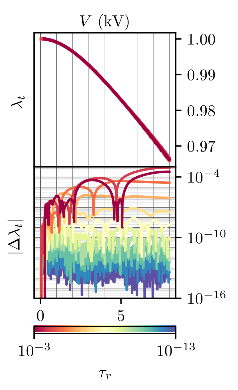
(c) Relative tolerance $\tau_{r}$

Figure 3: Voltage-stretch curve obtained using RK45. The voltage-to-stretch $f$ curves are plotted in solid lines and the stretch-to-voltage $f^{\dagger}$ curves are plotted in dotted lines. Different colors distinguish variations in $T$, $R$, and $\tau_{r}$.

5.1 Approximation using Numerical Integration Method

First, the solution is obtained by solving IVP using a numerical integration method. More specifically, an explicit Runge-Kutta method of order 5(4) [78], denoted as RK45, is employed as the numerical integrator. This approach integrates the equation with fifth-order accuracy while controlling the error utilizing a fourth-order accuracy method.

To obtain the voltage-to-stretch solution $f$, we initialize the process with $\lambda_{t}[0]=1$ and $V[0]=0$, and then iteratively determine $\lambda_{t}[n]$ using an integrator while varying $V[n]$ for $n\in\mathbb{Z}$. The stretch-to-voltage solution $f^{-1}$ is obtained through a similar procedure. Utilizing the RK45 integrator necessitates defining tolerances, as with many other numerical integration techniques. These tolerances, comprising an absolute tolerance ($\tau_{a}$) and a relative tolerance ($\tau_{r}$), serve to delineate the upper bound of local error estimates [77]. For instance, the voltage-to-stretch solver continues iterating until the solution converges, ensuring its error remains below $\tau_{a}+\tau_{r}\cdot|\hat{\lambda}_{t}|$. Conversely, the stretch-to-voltage process adheres to a similar criterion with $\tau_{a}+\tau_{r}\cdot|\hat{V}|$ for convergence.

Figure 3 (a) and (b) illustrates the solutions of equation (19) corresponding to various geometric parameters $T$ and $R$. Given that the stretch-to-voltage functions analyzed here approximate the inverse function of $f$, we use the notation $f^{\dagger}$ instead of $f^{-1}$. In each experiment, while varying the $T$ and $R$ values within their respective ranges, the other mechanical properties maintain the values detailed in Table 1. For reference, specific values such as $T=10^{-3.3}\approx 5\times 10^{-4}$ and $T=10^{-2.3}\approx 5\times 10^{-2}$ cover typical initial thicknesses of VHB^™ series, while $R=10^{-2.8}\approx 1.5\times 10^{-3}$ and $R=10^{-2.1}\approx 8\times 10^{-3}$ cover typical initial radii of the DEAs. The subplots (a) and (b) are simulated with $\tau_{a}=10^{-16}$ and $\tau_{r}=10^{-13}$. Subsequently, the numerical integrator consistently produces precise solutions for various parameters, with $f$ and $f^{\dagger}$ overlapping and exhibiting errors less than $10^{-11}$.

Figure 3 (c) shows the solutions corresponding to various tolerance $\tau_{r}$. The absolute tolerance values are set $\tau_{a}=\tau_{r}10^{-3}$. Since the tolerance determines the error of the solution, the figure shows that the difference between $f$ and $f^{\dagger}$ increases as the tolerance increases. However, enhancing efficiency remains a potential area for improvement, as the current approach necessitates a recursive update of solutions through numerical integration from the initial value to each target point. This leads to an approximated solution in an implicit form, estimating the output without the need for iteration or integration at each step.

Table 1 presents the notation and associated values for each parameter, conforming to the specifications for 3M^™ VHB^™ Tape 4910. The specific values align with Young’s modulus and permittivity, with detailed references available in [79] and [80].

5.2 Approximation using Neural Network

The methodology explored in Section 5.1 delineates a nonlinear yet time-invariant solution. Although several methods exist to approximate such functions — such as Taylor series expansion — we propose an implicit approximation through neural networks. In our investigation, we opt for an MLP as a specific choice to approximate a memoryless system. In consonance with the conceptual ethos presented in NEWT [72], we engineer the MLP with three layers and employ sinusoidal activation functions between these layers. Although the network architecture follows that of the conventional multilayer perceptions, a detailed architecture is succinctly outlined in Table 4.

The neural network is trained by simulating the voltage-stretch pair using the RK45 integrator. The training procedure is encapsulated in Algorithm 1. The voltage values within the training set are uniformly sampled from $V_{\text{min}}=0$ kV to $V_{\text{max}}=8$ kV. Each training iteration involves sampling voltage-stretch pairs, aggregating to a total batch size of $N=1024$.

The training procedures for $f_{\theta}$ and $g_{\theta}$ exhibit a slight variance: while $f_{\theta}$ is directly updated by gauging the loss using its output, $g_{\theta}$ is updated by measuring the loss after its amalgamation with $f_{\theta}$ as $f_{\theta}\circ g_{\theta}$. This section leverages the differentiable property of $f_{\theta}$, thereby employing the pre-trained and fixed $f_{\theta}$ to facilitate an end-to-end (E2E) training for $g_{\theta}$.

For training $f_{\theta}$, labeled pairs $\mathbf{V},\mathbf{\Lambda}$ are imperative. Therefore, we uniformly sample $\mathbf{V}$ within the range from $V_{\text{min}}$ to $V_{\text{max}}$ and simulate $\mathbf{\Lambda}$ using RK45 in each iteration. Conversely, as the objective for $g_{\theta}$ primarily involves learning to invert $f_{\theta}$, such simulation is deemed unnecessary for training $g_{\theta}$. Consequently, the training of $g_{\theta}$ omits the RK45 scheme, leading to nearly a twofold increase in training speed.

  Process TrainSimulator($K$, $V_{\textnormal{min}}$, $V_{\textnormal{max}}$, $N$, $\tau_{r}$, $\tau_{a}$):

  Initialize $f_{\theta}$

  for $k\in\mathbb{Z}_{K}$ do

           $\mathbf{V}\leftarrow\text{Uniform}(V_{\text{min}},V_{\text{max}},N)$

       // Sample $V$    

           $\mathbf{\Lambda}\leftarrow\text{RK45}(\mathbf{V},\tau_{r},\tau_{a})$

       // Simulate $\lambda$    

           $\mathbf{\hat{\Lambda}}_{f}\leftarrow f_{\theta}(\mathbf{V})$

       // Estimate $\hat{\lambda}$    

           $f_{\theta}\leftarrow f_{\theta}-\eta_{f}\|\mathbf{\Lambda}-\mathbf{\hat{\Lambda}}_{f}\|$

       // Update parameters    

  end for

        return $f_{\theta}$

      

  Process TrainCompensator($K$, $V_{\textnormal{min}}$, $V_{\textnormal{max}}$, $N$, $f_{\theta}$):

  Fix $f_{\theta}$; Initialize $g_{\theta}$

        $\lambda_{\text{min}}=\text{RK45}(V_{\text{min}})$; $\lambda_{\text{max}}=\text{RK45}(V_{\text{max}})$

  for $k\in\mathbb{Z}_{K}$ do

           $\mathbf{\Lambda}\leftarrow\text{Uniform}(\lambda_{\text{min}},\lambda_{\text{max}},N)$

       // Sample $\lambda$    

           $\mathbf{\hat{V}}_{g}\leftarrow g_{\theta}(\mathbf{\Lambda})$

       // Estimate $\hat{V}$    

           $\mathbf{\hat{\Lambda}}_{g}\leftarrow f_{\theta}(\mathbf{\hat{V}}_{g})$

       // Estimate $\hat{\lambda}$    

           $g_{\theta}\leftarrow g_{\theta}-\eta_{g}\|\mathbf{\Lambda}-\mathbf{\hat{\Lambda}}_{g}\|$

       // Update parameters    

  end for

        return $g_{\theta}$

      

Algorithm 1 Pseudo-code of the E2E training procedure

6 Evaluation

Section 5 introduces the modeling of the nonlinear deformation aspect, encompassing both the forward $f$ and the backward $f^{-1}$ behavior of the DEA. This section aims to assess the validity of the approximation as an inverse nonlinearity compensator $g$, also denoted as the waveshaping function in Figure 1.

Converting $f^{-1}$ into the waveshaping function is straightforward. Given our knowledge of $f$ and its inverse $f^{-1}$, the inverse nonlinearity compensator of $f$ can be represented by

$$g(x)=\frac{1}{\alpha}f^{-1}(a_{0}+a_{1}x)$$ (20)

as defined in equation (5). Here, $f$ simulates the stretch for a given voltage, while $f^{-1}$ determines the driving voltage required to achieve the desired stretch. Thus, rescaling the signal $x\in[-1,1]$ to the stretch $\lambda_{t}\in[\lambda_{\text{floor}},\lambda_{\text{ceil}}]\subset(0,1]$ suffices obtaining the inverse nonlinearity compensator $g$, as $f^{-1}$ indicates the required voltage for the specified stretch.

The affine transformation by $a_{0}$ and $a_{1}$ rescales $x\mapsto\lambda_{t}$, where $a_{0}$ and $a_{1}$ are determined by the driving voltage range. Fixing the AC and DC components of the driving voltage ($V_{\text{pp}}$ and $V_{\text{dc}}$, respectively), where $V_{\text{min}}\leq V_{\text{floor}}=V_{\text{dc}}-V_{\text{pp}}/2$ and $V_{\text{dc}}+V_{\text{pp}}/2=V_{\text{ceil}}\leq V_{\text{max}}$, sets the range of stretch as $\lambda_{\text{floor}}=f(V_{\text{floor}})$ and $\lambda_{\text{ceil}}=f(V_{\text{ceil}})$, along with determining $a_{0}$ and $a_{1}$. To assess how accurate the approximation $f^{\dagger}$ is in comparison to $f^{-1}$, we evaluate their proximity in the context of the INC, by replacing $f^{-1}$ in equation (20) with $f^{\dagger}$. For the particular choice of the coefficients, we refer the readers to B.2.

6.1 Baselines

Prior research aiming to mitigate acoustical distortion in DEAs has often relied on the square root function [12]. When considering the linear elastic model, employing the square root on the voltage signal is intuitive (refer A). However, in our case of nonlinear elastic deformation, more suitable adaptations are necessary. Hence, we propose to benchmark our approach against two baselines: a trainable power function and a piecewise polynomial interpolation.

6.1.1 Power Function Fitting

Our first baseline involves a power function, where the power exponent becomes a trainable parameter. This can be viewed as an extension of the square-root compensation advocated by Heydt et al. [12]. The power function, characterized by fitted parameters $\theta_{j}^{(1)}$, is articulated as follows:

$$f^{(1)}=\theta_{1}^{(1)}\left(|\theta_{2}^{(1)}(1-\lambda_{t})+\theta_{3}^{(1)}|\right)^{\theta_{0}^{(1)}}+\theta_{4}^{(1)}$$ (21)

Affine transformations precede and succeed in the power operation to fine-tune the scale between stretch and voltage. To ensure numerical stability, an absolute operator ($|\cdot|$) is applied before the power operation. We denote the equation (21) as Power Function Fitting (PFF). For a more comprehensive understanding of the other families of trainable functions as baselines, we direct interested readers to C.

6.1.2 Piecewise Quartic Interpolation

Long-standing efforts have been made to interpolate Runge-Kutta solutions [81, 82]. From this line of work, we compare our method with a piecewise quartic interpolation (PQI) [83]. The interpolation is performed in a piecewise manner, wherein each segment of the solution is approximated using a quartic polynomial. While it is possible to tune the accuracy of PQI by adjusting the tolerance in the RK45, we fix $\tau_{r}=10^{-6}$ and $\tau_{a}=10^{-9}$ for evaluation. The selected values are thoughtfully curated to ensure an equitable comparison, taking into account computational expenses (refer to B.4 for further details).

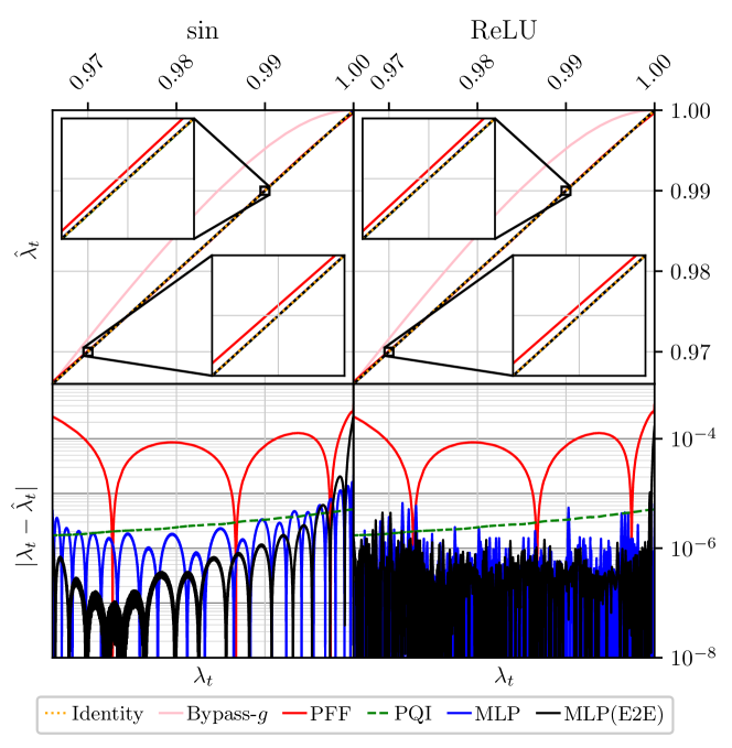
Figure 4: Plot of $\hat{\lambda}_{t}=f\circ f^{\dagger}$ and $|\lambda_{t}-\hat{\lambda}_{t}|$ against $\lambda_{t}$.

6.2 Evaluation metric

We assess the outcomes using three key metrics: log of the $\ell_{1}$-norm of stretch difference ($\log\ell_{1}$), $\ell_{1}$-norm of the log magnitude spectrogram difference ($\ell_{1}^{\text{STFT}}$), and signal-to-distortion ratio (SDR). The log of the $\ell_{1}$-norm of stretch difference is calculated as

$$\log\ell_{1}(\hat{\lambda}_{t},\lambda_{t}):=\log_{10}\|\hat{\lambda}_{t}-\lambda_{t}\|_{1}$$ (22)

where $\hat{\lambda}t=f(\hat{x})$ represents the estimated stretch of the compensated signal $\hat{x}$. To calculate $\log\ell_{1}$, we linearly probe $x$ within the range $x\in[V_{\text{min}},V_{\text{max}}]$. However, the remaining metrics are applied to evaluate sinusoidal signals specifically. For instance, the sinusoid $x[n]=V_{\text{dc}}+(V_{\text{pp}}/2)\sin(\omega n)$ with $V_{\text{dc}}=6$ kV and $V_{\text{pp}}=3$ kV varies its frequency within the range between 0 to $12$ kHz. The sampling rate $f_{s}$ is set to 48 kHz. Upon obtaining the estimated $\hat{\lambda}_{t}[n]=f(\hat{x}[n])$ for the sinusoidal $\hat{x}$, we compare the log magnitude difference of the spectrograms as

$$\ell_{1}^{\text{STFT}}(\hat{\lambda}_{t},\lambda_{t}):=\left\|10\log_{10}\left|\frac{\text{STFT}(\hat{\lambda}_{t})}{\text{STFT}(\lambda_{t})}\right|^{2}\right\|_{1}$$ (23)

and the signal-to-distortion ratio as

$$\text{SDR}(\hat{\lambda}_{t},\lambda_{t}):=10\log_{10}\frac{\|\lambda_{t}\|_{2}^{2}}{\|\hat{\lambda}_{t}-\lambda_{t}\|_{2}^{2}}$$ (24)

which represents the ratio of $\ell_{2}$-norms between the reference signal $\lambda_{t}$ and the distortion $\hat{\lambda}_{t}-\lambda_{t}$ in dB scale. Among the three indicators, SDR is the only metric where a larger value indicates superior performance, while for the rest, a smaller value signifies better performance.

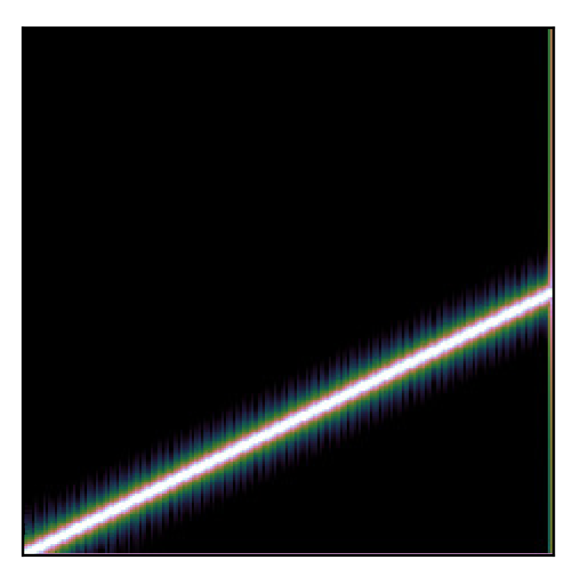
(a) Original

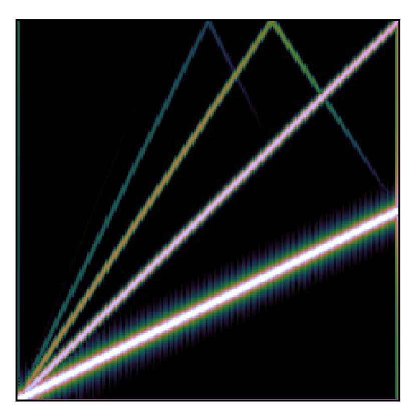
(b) Bypass-$g$

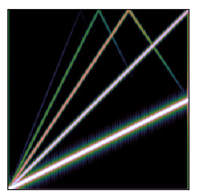
(c) HFF

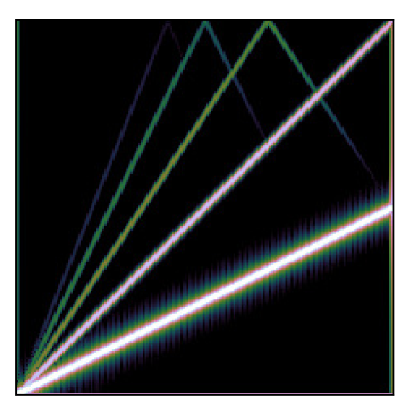
(d) LFF

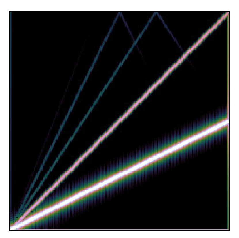
(e) PFF

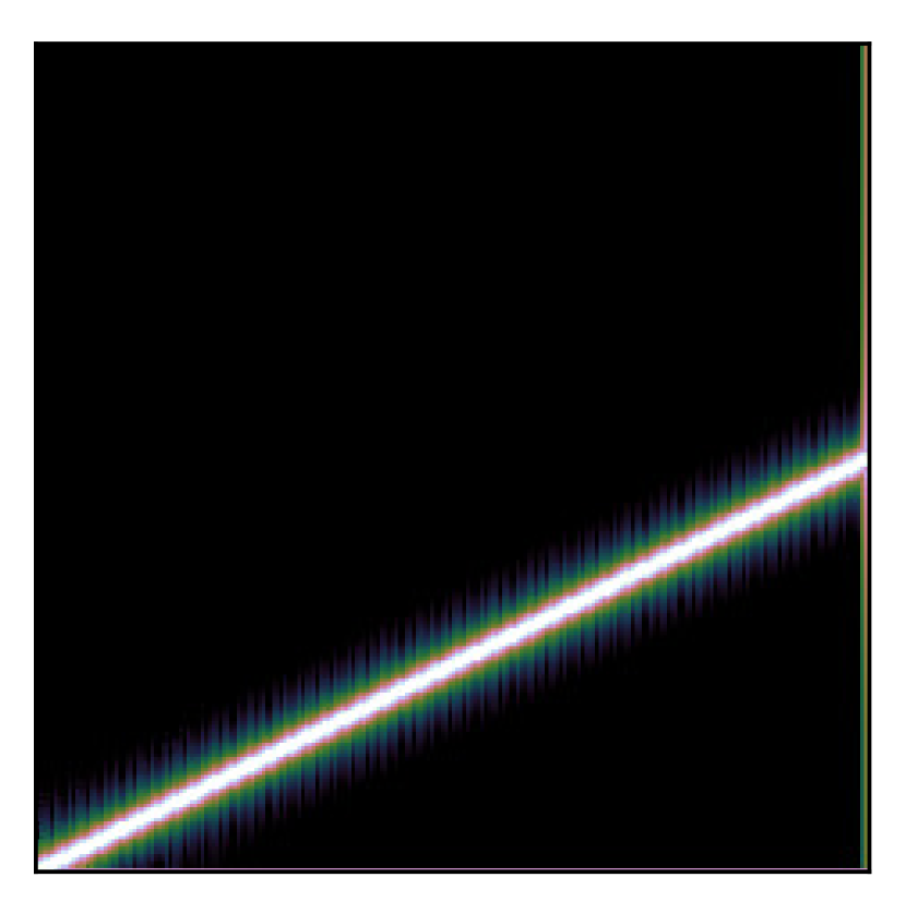
(f) PQI

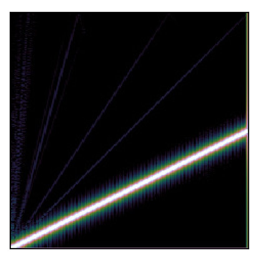
(g) MLP(ReLU)

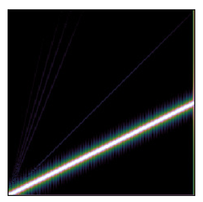
(h) MLP(sin)

Figure 5: Spectrograms of the experimented sinusoidal signals. Patch (a) shows the spectrogram of the original input as the pure sinusoidal sweep signal. Patches (b)-(h) show the spectrograms of the simulated output signals, where (b) shows the output without any compensation and patches (c)-(h) show the outputs with different inverse nonlinearity compensators.

6.3 Evaluation results

The presented visual depiction in Figure 4 illustrates the waveshaping function $\alpha g(x)=f^{\dagger}(a_{0}+a_{1}x)$ combined with the deformation function $f$. The case where no compensation is applied is labeled as Bypass-$g$. For all $f^{\dagger}$ models, the fixed forward deformation function $f$ adheres to PQI with $\tau_{r}=10^{-13}$. A detailed discussion concerning this choice is available in B.1.

Each column showcases diverse results for nonlinear activations in MLPs, utilizing sin and ReLU activations for the left and right columns, respectively. The top row illustrates $f\circ f^{\dagger}(\lambda_{t})$ against $\lambda_{t}$, portraying the proximity to the identity mapping (indicated by Identity) and indicating the closeness of $f^{\dagger}\approx f^{-1}$. Bypass-$g$, where no compensation occurs ($f^{\dagger}=\textbf{1}$), is plotted for a reference. Although PFF exhibits compensation performance yielding $f\circ f^{\dagger}$ close to the identity, the improvement is marginal compared to that of PQI or MLP. The subsequent bottom row in Figure 4 shows the errors $|\lambda_{t}-f\circ f^{\dagger}(\lambda_{t})|$, represented on a logarithmic scale.

While PQI consistently demonstrates errors in $|\lambda_{t}-f\circ f^{\dagger}(\lambda_{t})|$ against $\lambda_{t}$, its average error surpasses that of MLPs. However, despite this discrepancy, PQI exhibits fewer harmonics, particularly when compared to MLP(ReLU). This divergence becomes more pronounced when examining the scores in Table 2: MLP(ReLU) outperforms PQI in $\log\ell_{1}$ with a margin of 0.34, but displays inferior performance in $\ell_{1}^{\text{STFT}}$ and SDR. We attribute this phenomenon carefully to the consistency in the error. More details supporting this inference can be found in E.

Among the MLPs, an ablation study on the training method is conducted, where the MLP is directly trained from data simulated using RK45 (marked MLP). Algorithm 2 delineates the detailed training procedure for this study. Conversely, the proposed MLP(E2E), trained via Algorithm 1, demonstrates superior performance in average stretch regions. Nevertheless, MLP(E2E) with sin activation exhibits reduced accuracy in small strain regions ($\lambda_{t}>0.99$). In contrast, MLP(E2E) with ReLU activation shows the best $\log\ell_{1}$ score (as detailed in Table 2). However, ReLU introduces non-smoothness, evident in the jagged error plot, warranting a deeper examination through objective evaluation scores.

Table 2: Evaluation results. Bold texts indicate the best scores. White texts indicate the less performant scores compared to Bypass-$g$.

$g(x)$	$\log\ell_{1}$	Unnormalized		Normalized
		$\ell_{1}^{\text{STFT}}$	SDR	$\ell_{1}^{\text{STFT}}$	SDR
Bypass-$g$	-1.7431	0.2060	74.91	0.4702	65.24
HFF (§C.1.2)	-3.5763	0.2905	76.51	0.6474	61.76
LFF (§C.1.1)	-3.7179	0.2101	77.41	0.4551	63.68
PFF (§6.1.1)	-4.0731	0.1020	82.79	0.2784	67.18
PQI (§6.1.2)	-5.5426	0.0001	112.56	0.0004	111.12
MLP(Identity)	-4.5614	0.0040	101.95	0.0381	85.51
MLP($\tanh$)	-5.6983	0.0001	128.42	0.0006	112.91
MLP(ReLU)	-5.8888	0.0003	129.35	0.0005	114.85
MLP($\sin$)	-5.3744	0.0001	133.01	0.0003	116.88

Table 2 provides a comparative analysis of objective scores, color-coded to depict performance from the worst (darkest cells) to the best (lightest cells) among $f^{\dagger}$ models. Apart from the proposed MLP(sin) model, the table includes an ablation study on each MLP’s nonlinearity functions (MLPs, HFF, LFF, and PFF), all trained using E2E as per Algorithm 1.

The $\log\ell_{1}$ score reveals that MLP(ReLU) attains the superior performance. This aligns with the findings depicted in Figure 4, as the average $|\lambda_{t}-\hat{\lambda}_{t}|$ for MLP(ReLU) is lower, especially in small strain regions. However, when subjected to evaluation using sinusoidal signals, MLP(sin) excels notably in both $\ell_{1}^{\text{STFT}}$ and SDR scores, demonstrating its prowess in both normalized and unnormalized scenarios. This disparity in performance suggests that while MLP(ReLU) converges better, MLP(sin) better suppresses distortions, showcasing fewer harmonic artifacts. This is analogous to why PQI, despite its inferior $\log\ell_{1}$ score, yields less harmonic than MLP (ReLU). Further information can be found in E.

Notably, HFF and LFF, despite significantly improving the $\log\ell_{1}$ score, perform worse than the Bypass-$g$ case in some indices, indicating that incomplete compensation might exacerbate distortions. PFF outperforms HFF or LFF, yet MLP(Identity), equipped solely with a Softplus as an activation function, surpasses PFF across all measures, reaffirming the approximation capability of MLPs. However, PQI consistently outperforms MLP(Identity) across indices, closely trailing MLP(sin) with minor differences observed in $\ell_{1}^{\text{STFT}}$, yet displaying some shortcomings in SDR.

We also conduct a comparative analysis between the results obtained from the unnormalized stretch and the min-max normalized stretch signals. The unnormalized stretch primarily consists of values within the range of $[0.96,1.0]$ in the signal. Given the limited range of stretch values, distinguishing between methods might pose some subtleties. However, normalization proves to be instrumental in highlighting differences between the methods. This emphasizes that MLP(sin) outperforms others, particularly among those equally ranked first in the unnormalized $\ell_{1}^{\text{STFT}}$ metric. These objective scores are further supported by an alignment with the actual samples.

Figure 5 presents spectrograms of compensated outputs, showcasing harmonics aligned with results in Table 2. Notably, MLP(sin) alongside PQI predominantly displays mere harmonics in its estimated spectrogram. Although subtle, MLP(ReLU) manifests a discernible harmonic, while the remaining baselines distinctly present clear harmonics. This again highlights the use of the periodic activation functions in MLPs.

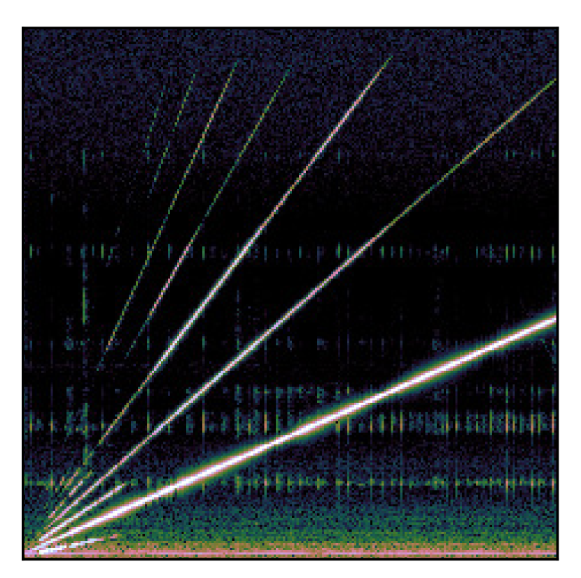
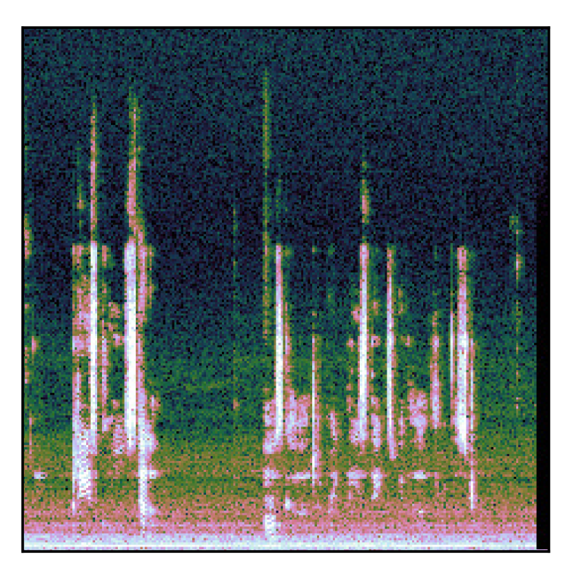
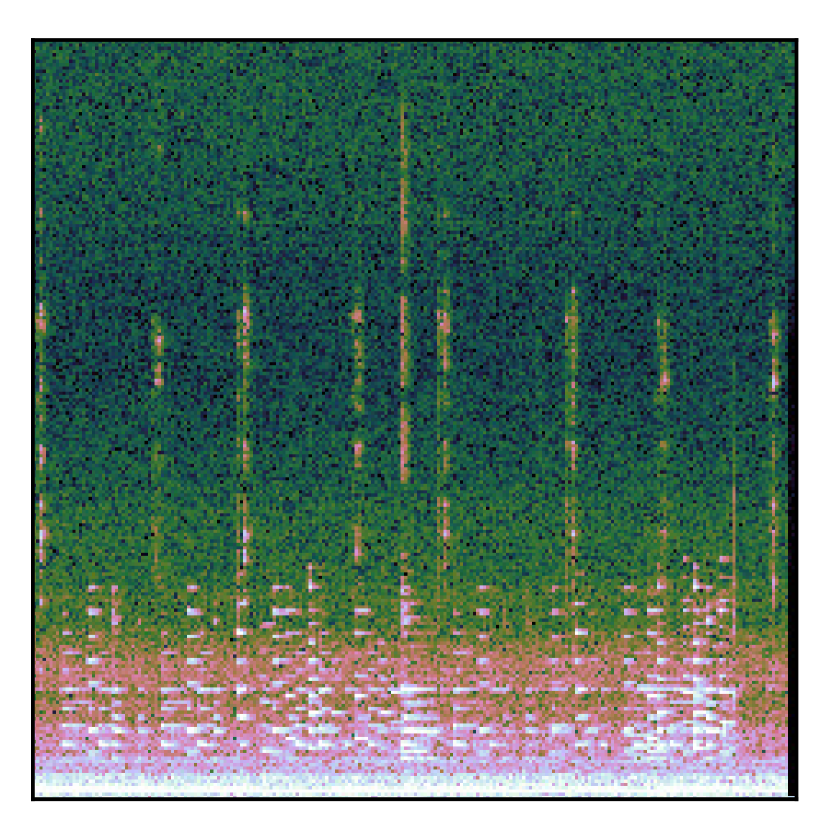
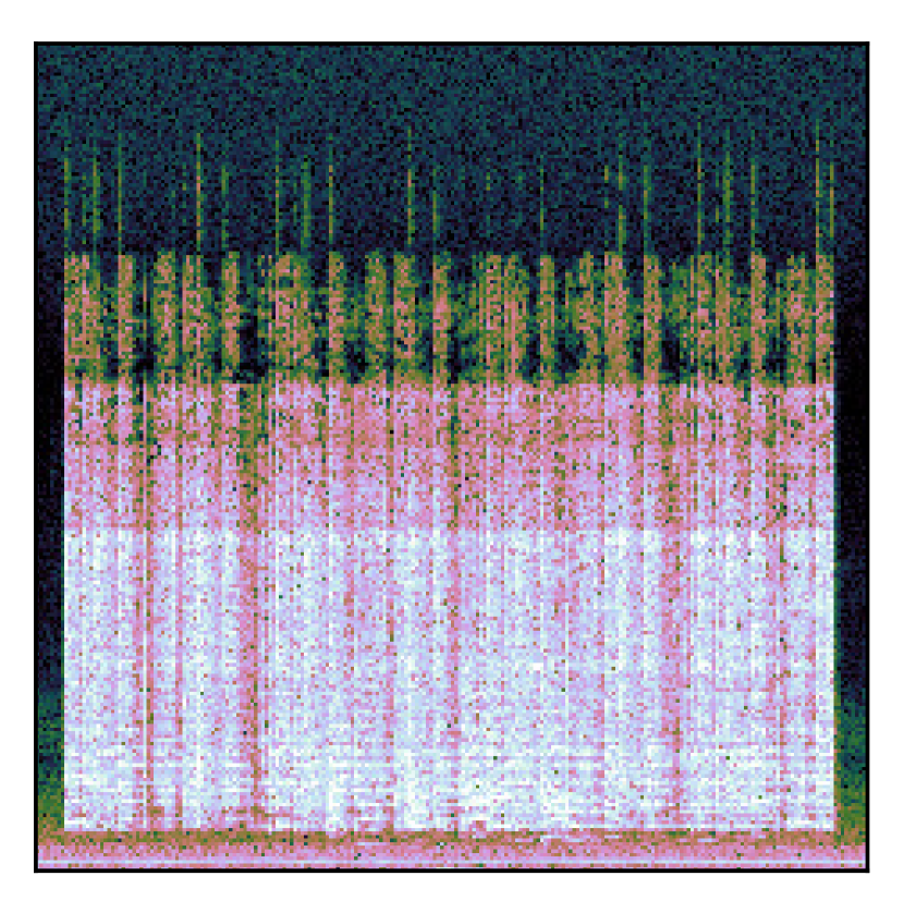
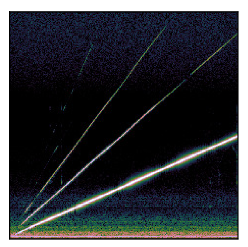
(a) Sinusoids

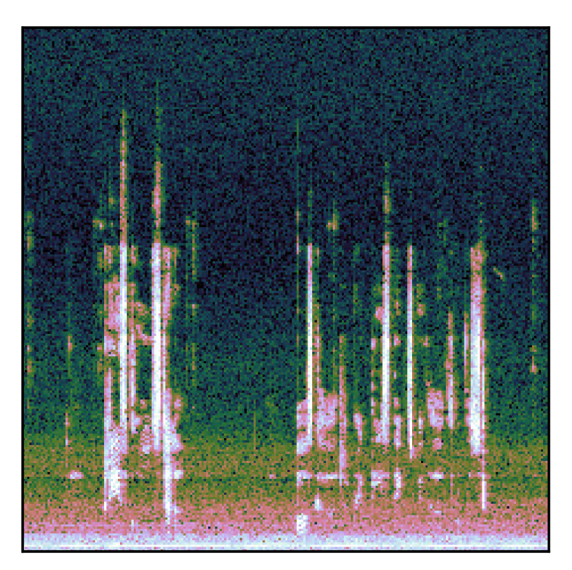
(b) Speech

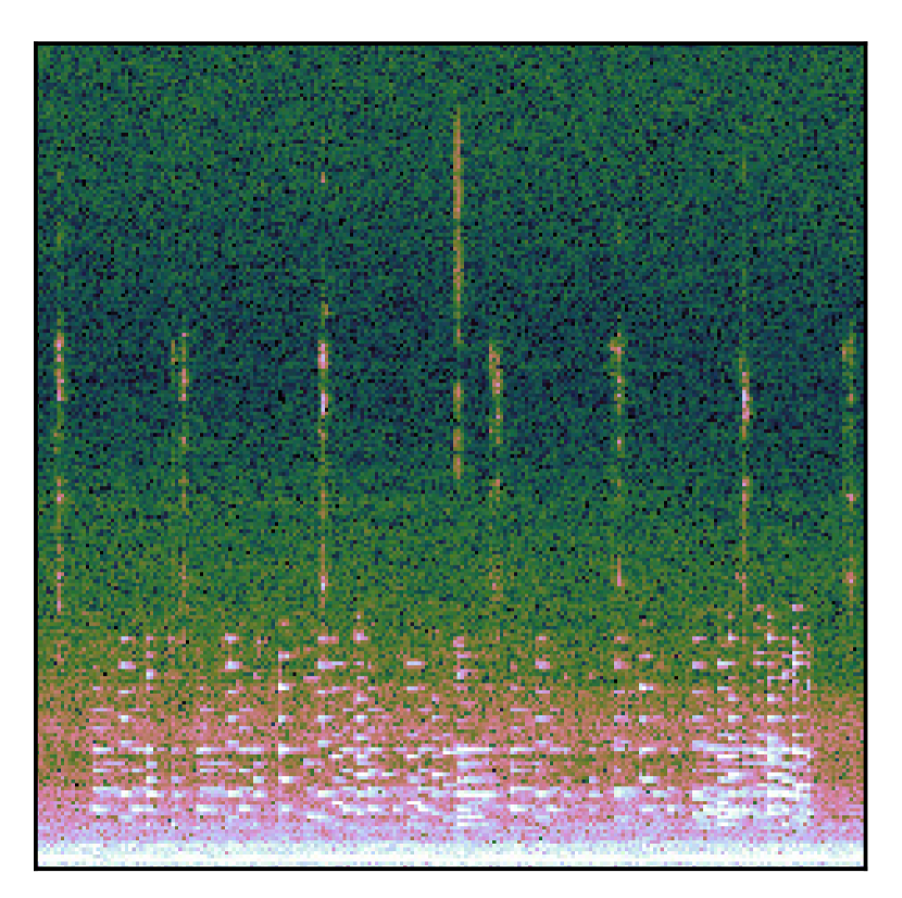
(c) Piano music

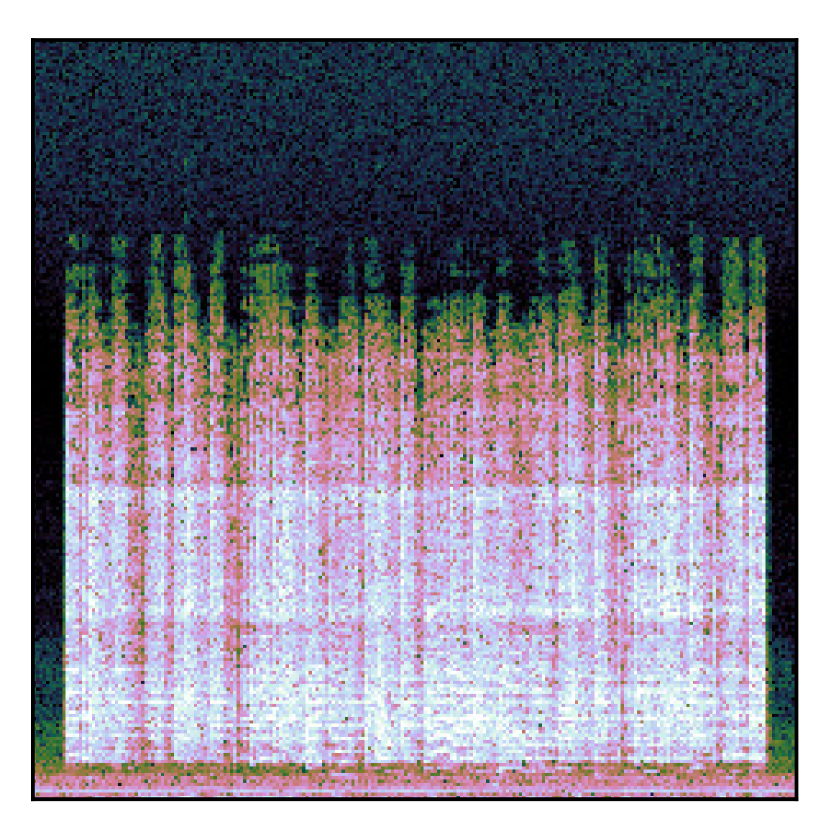
(d) Electronic music

Figure 6: Spectrograms of the measured sound actuated using DEA. The signals without compensation are plotted on the top row. The signals compensated with MLP(sin) are plotted on the bottom row.

To further validate the effectiveness of the compensation, we conduct an evaluation of MLP(sin) on real-world DEAs. Given that our study involves simulations and compensations based on idealized DEAs, it is anticipated that the compensation results obtained from the manufactured DEAs might display discrepancies when compared to simulated outcomes. For a comprehensive understanding of the equipment configuration, we direct readers to F for detailed information. Diverse signals encompassing sinusoidal sweeps, speech, and musical inputs were pre-compensated and amplified before being applied to the DEA.

Figure 6 depicts spectrograms representing the measured signals. Despite potential measurement errors and background noise, the spectrogram demonstrates a noteworthy reduction in harmonics following calibration compared to pre-calibration. This observation holds even in cases where the original signal contains multiple frequency components, such as speech or music, revealing a significant improvement post-calibration. This enhancement is particularly evident in a sine sweep input, but it becomes even more pronounced when dealing with signals containing a broader spectrum of frequencies. For the sine sweep input, compensation using MLP(sin) yielded a result of 2.1% for Total Harmonic Distortion (THD), marking a significant enhancement from the value of 14.89% for the case without any compensation.

7 Conclusion

This study addresses the nonlinear deformation induced by dielectric actuation in pre-stressed ideal dielectric elastomers. The paper establishes a comprehensive understanding by formulating a nonlinear ordinary differential equation based on the hyperelastic deformation, elucidating the intricate solution between voltage and stretch. By utilizing numerical integration and neural networks, the solutions are efficiently approximated, without losing their accuracy. The methods are evaluated through inverse nonlinearity compensation tasks showcasing the efficacy of the end-to-end trained MLPs. The demonstrated effectiveness of these approximations, notably in minimizing harmonic distortions when utilized in acoustic actuation, underscores the significance of this research in enhancing the performance of such materials. Furthermore, the outcomes emphasize the potential of employing neural networks for addressing nonlinearities, thereby paving the way for improved acoustic applications of dielectric elastomers.

Appendix A Linear elastic model

In this section, we provide an analytic relation between the voltage $V$ and the thickness strain $\epsilon_{t}=\lambda_{t}-1$. While this is a different line of work than the main paper, which deals with hyperelastic deformations, the material in this section provides background on how the polynomial baselines (PFF, PQI) came about, as well as insight into how an analytic form of an inverse nonlinear compensator can be obtained for DEA with linear elasticity.

The effective pressure $P_{E}$ applied to the elastomer, i.e. the Maxwell stress, is expressed as

$$P_{E}=\varepsilon_{0}\varepsilon_{r}\cdot{E}^{2}=\varepsilon_{0}\varepsilon_{r}\cdot\left(\frac{{V}}{t}\right)^{2}$$ (25)

where ${E}$ denotes the electric field. Assuming the balance between the electrostatic pressure (25) and the elastic pressure of the film, the thickness strain can be written as

$$\epsilon_{t}=-\frac{P_{E}}{Y}=-\varepsilon_{0}\varepsilon_{r}\left(\frac{{V}}{t}\right)^{2}Y^{-1},$$ (26)

where $Y$ denotes the Young’s modulus of the polymer. Assuming linear elastic deformation with small strains (less than 10%), substitute $t$ in (26) by $T(1+\epsilon_{t})$ and obtain

$$\epsilon_{t}^{3}+2\epsilon_{t}^{2}+\epsilon_{t}=-\epsilon_{0}\epsilon_{r}\frac{{V}^{2}(t)}{YT^{2}}.$$ (27)

For convenience, put

$$\epsilon_{T}(t)=-\epsilon_{0}\epsilon_{r}\frac{{V}^{2}(t)}{YT^{2}}.$$ (28)

An analytic solution for (27) can be expressed, under restriction $-\frac{1}{3}<\epsilon_{t}\leq 0$:

$$\epsilon_{t}(t)=-\frac{2}{3}+\frac{1}{3}\left(E(t)+\frac{1}{E(t)}\right),$$ (29)

with denoting

$$E(t)=\left[\frac{1}{2}\left\{\left(2+27\epsilon_{T}(t)\right)+\left(\left(2+27\epsilon_{T}(t)\right)^{2}-4\right)^{\frac{1}{2}}\right\}\right]^{\frac{1}{3}}.$$ (30)

Note that (29) is one of the three solutions for the cubic equation (27), which lies in the range of our interest. For the restriction range of (29), the bound for $\epsilon_{t}\leq 0$ is implied by ${V}\geq 0$. To see the bound for $\epsilon_{t}>-\frac{1}{3}$, find the derivatives

$$\frac{\partial\epsilon_{t}(t)}{\partial\epsilon_{T}}=\frac{1}{3\epsilon_{t}^{2}(t)+4\epsilon_{t}(t)+1}.$$ (31)

Since $3\epsilon_{t}^{2}(t)+4\epsilon_{t}(t)+1=(3\epsilon_{t}(t)+1)(\epsilon_{t}(t)+1)\to+0$ as $\epsilon_{t}(t)\to-\frac{1}{3}+0$, the derivative $\frac{\partial\epsilon_{t}(t)}{\partial\epsilon_{T}}\to+\infty$. This implies that as the amount of thickness reduction reaches $\frac{1}{3}$ of the initial thickness, the membrane becomes so unstable that its thickness breakdowns or violates other assumptions [13, 26].

Appendix B Details of the Evaluation

B.1 Choice of the forward deformation model

The approximate solution was used because it is difficult to obtain the solution when applying a signal in addition to numerical stability to use RK45 as it is. While it is possible to use a trained MLP model as the forward $f$, we do not see a significant performance improvement compared to the PQI, where the latter is more convenient in tuning its accuracy through adjusting $\tau_{r}$.

B.2 Details on the inverse nonlinearity compensation function

As discussed in section 6, the inverse nonlinearity compensator of $f$ can be represented using an affine transformation of $f^{-1}$. For evaluation, we utilize equation (20) with $\alpha=1000$, $a_{1}\approx-0.0341325$, and $a_{0}\approx 0.9999924$. This particular choice of parameters is set to preserve the stretch at $V_{\text{min}}$ and $V_{\text{max}}$, i.e., $\lambda_{\text{min}}=f(V_{\text{min}})=f(\alpha g(V_{\text{min}}))$ and $\lambda_{\text{max}}=f(V_{\text{max}})=f(\alpha g(V_{\text{max}}))$.

B.3 Training strategy

Some may wonder about the efficacy of end-to-end training of $g_{\theta}$ as in Algorithm 1, as it is also possible to simulate the paired $(V,\lambda_{t})$ for training $g_{\theta}$. To be more specific, Algorithm 2 shows the pseudo-code of this training procedure. The performance of $g_{\theta}$s trained through this pseudo-code is already shown in Figure 4 (labeled MLP). As the figure shows, no significant improvement was found through this training strategy, and the performances were typically worse than the models undergone E2E training.

  Process Train($K$, $V_{\textnormal{min}}$, $V_{\textnormal{max}}$, $N$):

  Initialize $f_{\theta},g_{\theta}$

  for $k\in\mathbb{Z}_{K}$ do

           $\mathbf{V}\leftarrow\text{Uniform}(V_{\text{min}},V_{\text{max}},N)$

       // Sample $V$    

           $\mathbf{\Lambda}\leftarrow\text{RK45}(\mathbf{V})$

       // Simulate $\lambda$    

           $\mathbf{\hat{\Lambda}}\leftarrow f_{\theta}(\mathbf{V})$

       // Estimate voltage-to-stretch    

           $\mathbf{\hat{V}}\leftarrow g_{\theta}(\mathbf{\Lambda})$

       // Estimate stretch-to-voltage    

     $f_{\theta}\leftarrow f_{\theta}-\eta_{f}\|\mathbf{\Lambda}-\mathbf{\hat{\Lambda}}\|$

     $g_{\theta}\leftarrow g_{\theta}-\eta_{g}\|\mathbf{V}-\mathbf{\hat{V}}\|$

  end for

        return $f_{\theta},g_{\theta}$

      

Algorithm 2 Pseudo-code of the training procedure using RK45 simulation as the paired label simulator. The training procedure for $f_{\theta}$ is identical to the Algorithm 1.

B.4 Computational efficiency

We also compare the computation time between RK45, PQI, and MLP(sin). Figure 7 summarizes the results. To measure the computational time, we fix the hardware to either a single CPU thread (AMD Ryzen 5 3600 @2.2GHz) or a single GPU (RTX 2060). The times are averaged over a 1000 repeated measurements.

Not surprisingly, MLP shows that its time does not vary with tolerance, while RK45 and PQI show a slowdown in computation as tolerance becomes smaller. The number of samples used to measure the simulation time under $\tau_{r}$ is $10^{3}$. Smaller values of tolerance usually increase the number of iterations required for the solution to converge, so it’s not surprising that RK45 slows down. However, it is interesting to see that the computation time of PQI increases with tolerance, even though no internal iterations are required.

Conversely, for compute time as a function of sample count, RK45 does not show a significant slowdown, while for PQI and RK54, the slowdown becomes apparent as soon as the number of samples exceeds $10^{3}$. While it is not surprising that the total computation time increases as the number of samples increases, it is impressive to see that they are slower than the RK45 solver once the number of samples exceeds $10^{4}$. We speculate that memory overhead may play a role in this slowdown.

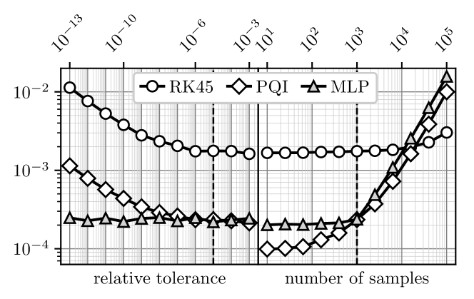
Figure 7: computational time comparison

Appendix C Baseline details

The baselines are trained using Algorithm 1 where the trainable parameters are defined according to the specific formulations, such as PFF (21). In addition to PFFs using power functions, we also validate the compensation capabilities with trainable forms for other kinds of functions. As two examples of such functions, this section provides some more details about LFF and HFF.

Table 3: Initial parameters

Model	$\theta_{0}$	$\theta_{1}$	$\theta_{2}$	$\theta_{3}$	$\theta_{4}$
Baseline1	$0.5$	$3\times 10^{3}$	0	$1\times 10^{3}$	0
Baseline2	$0.3$	$1\times 10^{3}$	1	$2\times 10^{3}$	0
Baseline3	-	$1\times 10^{4}$	0	$9\times 10^{2}$	0

C.1 Functions with Trainable Parameters

As a different kind of compensation function from the power function, we consider logarithmic and hyperbolic families. With a proper design of choice and initialization, such functions can also compensate for the deformation $f$ to some extent. Exemplar identity plots $f\circ f^{\dagger}$ for each baseline $f^{\dagger}$ are plotted in Figure 8. Based on the observations in Figure 8, we initialize the trainable parameters of each function as Table 3 and fine-tune them to compensate better.

(a) PFFs

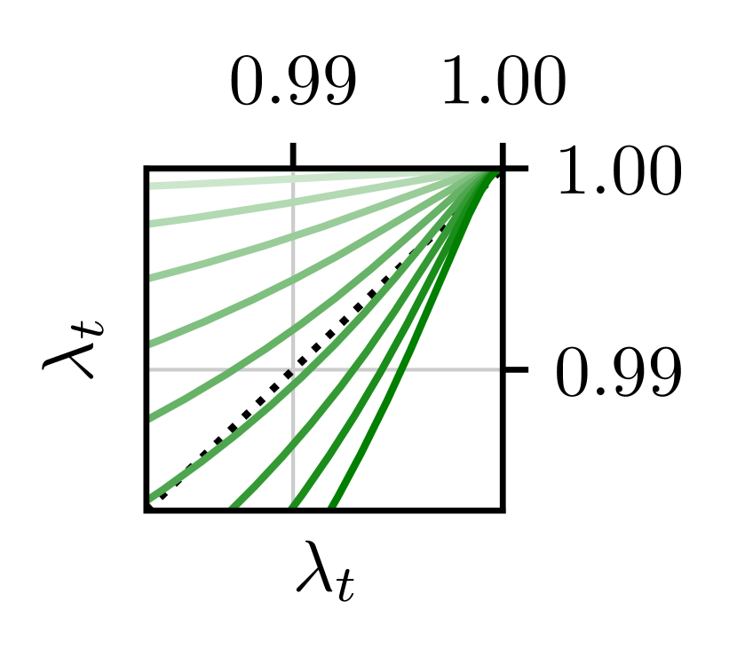
(b) LFFs

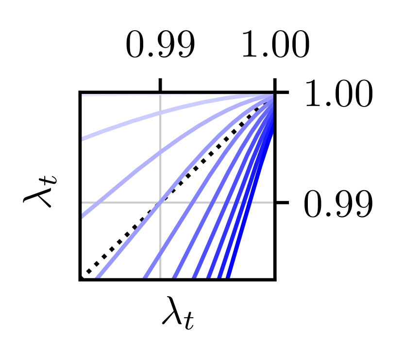
(c) HFFs

Figure 8: Plot of $f\circ f^{\dagger}$. $\beta$ are swept from $10^{2}$ to $4\times 10^{3}$ (curves for the larger $\beta$ are plotted in higher color intensity.) (a) $f^{\dagger}=10^{3}\sqrt{\beta_{1}(1-\lambda_{t})}$, the first baseline as a square-root function. (b) $f^{\dagger}=\beta_{2}\log(10^{3}(1-\lambda_{t}^{0.3})+1)$, the second baseline as a logarithmic function. (c) $f^{\dagger}=10^{4}\tanh(\beta_{3}(1.002-\lambda_{t})/45)$, the third baseline as a tanh function.

C.1.1 Logarithmic function

The logarithmic function fitting (LFF) is defined as follows.

$$f^{(2)}=\theta_{1}^{(2)}\log\left(\theta_{2}^{(2)}\cdot\left(\theta_{3}^{(2)}-\lambda_{t}^{\theta_{0}^{(2)}}\right)+1\right)+\theta_{4}^{(2)}$$ (32)

Some might wonder why there also is a trainable power operator $\theta_{0}^{(2)}$. The difference is marginal between fixing $\theta_{0}^{(2)}=1$ and updating it, but we use this power-ed version since it fits slightly better looking into Figure 8 (b).

C.1.2 Hyperbolic function

We also study a hyperbolic family as the compensation function.

$$f^{(3)}=\theta_{1}^{(3)}\tanh\left(\frac{\theta_{2}^{(3)}}{45}(1.002-\lambda_{t})+\theta_{3}^{(3)}\right)+\theta_{4}^{(3)}$$ (33)

As $\tanh(x)=(e^{x}-e^{-x})/(e^{x}+e^{-x})$, this can also be viewed as a demonstration of an exponential family, but we denote this method as Hyperbolic Function Fitting (HFF). Although we explored other families of trainable functions, such as logarithmic and hyperbolic functions, we observed no substantial improvement compared to the power function. Consequently, these results are excluded from the evaluation section.

Appendix D Training Details

In training the models, both $f_{\theta}$ and $g_{\theta}$ undergo training for 1M steps utilizing the Adam optimizer [84]. The learning rates are set to $\eta_{f}=10^{-6}$ and $\eta_{g}=10^{-5}$ for $f_{\theta}$ and $g_{\theta}$, respectively, and are subsequently reduced by a factor of $0.9$ every 20k steps. This training configuration is identically applied to train MLPs and the baselines. Table 4 summarizes the neural network architecture used in this study.

Table 4: Neural network architecture

Layer	Input dim.	Output dim.	Operations
1	1	512	Linear, sin, LayerNorm
2	512	512	Linear, sin, LayerNorm
3	512	1	Linear, Softplus

Appendix E More on activation function

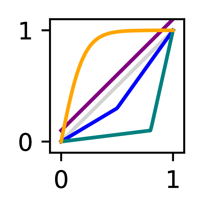
(a) Waveshaper

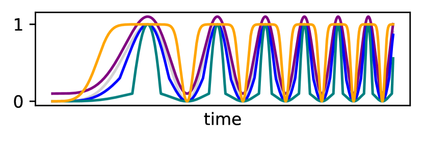
(b) Waveform after waveshaping

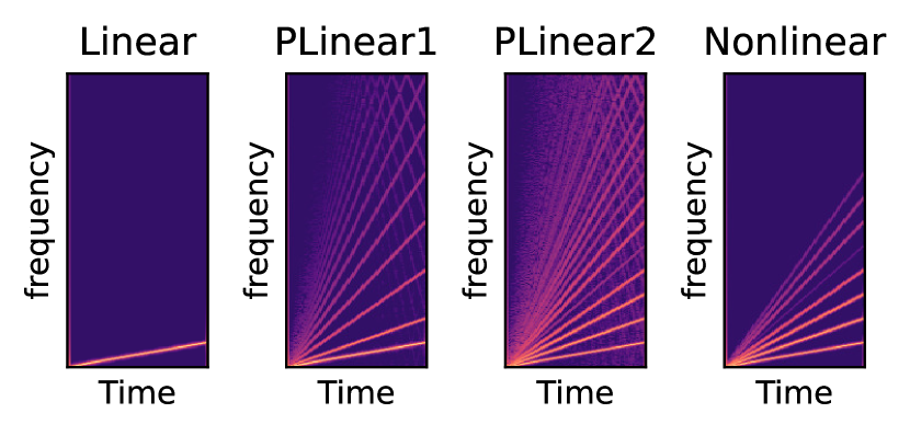
(c) Log magnitude spectrogram

Figure 9: Examples of waveshaping sinusoids.

This section studies the smoothness of a waveshaping function on the harmonic distortion. For some, it could be obvious that the sinusoids wave-shaped by non-smooth functions — which require Fourier series approximation up to the infinite number of orders in theory — can raise many numbers of harmonics. Yet, we expand more on this with some toy experiments to see the same conclusion in terms of the objective metrics and relate it with the experiment results in section 6.3.

To study the effect of the smoothness, we compare three waveshaping functions: two piecewise linear functions and a nonlinear function. For the nonlinear function, we use the hyperbolic tangent $h(x)=\tanh(5x)$. The waveshaping functions are plotted in Figure 9 (a), where a light gray line ( ) indicates an identity function. Then, we apply a sinusoidal sweep with its amplitude ranging from 0 to 1. The original sinusoid is plotted using a light gray line in the subplot (b), which only visualizes the front 0.08 sec of the whole signal. The fundamental frequency is swept from 0 to 2 kHz for 1 sec, with a sampling rate of 48 kHz.

Figure 9 (c) shows the spectrograms of the waveshaping-distorted signals $h(x)$ within -100 dB to +10 dB. As it appears in the spectrograms, the signals distorted by piecewise linear functions show more harmonics than the signal distorted by the $\tanh$ function.

Table 5: Objective score for the waveshaping examples

Method	$\log\ell_{1}$	$\ell_{1}^{\text{STFT}}$	SDR
Linear	1.00	0.19	15.7
PLinear1	1.00	5.10	16.2
PLinear2	1.54	13.6	4.93
Nonlinear	1.55	3.56	4.89

To compare this more rigorously, we measure the objective scores between the sinusoid $x$ and the waveshaping-distorted $h(x)$. Table 5 summarizes the scores. As it is shown in Figure 9 (a), $\log\ell_{1}$ measures the smallest score for PLinear1; which is the closest to the identity function. PLinear2 and Nonlinear $\tanh$ are designed to have similar $\log\ell_{1}$ scores. The SDR scores show a similar tendency as it is measured at the sample level: looking into (b), the distance from the original sinusoid is the smallest for the PLinear1, and vice versa.

However, the spectral scores $\ell_{1}^{\text{STFT}}$ show clearly different results. Although PLinear2 and Nonlinear show similar $\log\ell_{1}$ (and SDR either), $\ell_{1}^{\text{STFT}}$ score of PLinear2 is almost 10 dB higher than that of Nonlinear. Also, even though PLinear1 shows the lowest $\log\ell_{1}$, its $\ell_{1}^{\text{STFT}}$ score is worse than that of Nonlinear with an amount of approximately 1.6 dB. This $\ell_{1}^{\text{STFT}}$ supports the observation in Figure 9 (c) that the signals distorted by piecewise linear functions show more harmonics than the signal distorted by the $\tanh$ function.

These results again highlight that the closeness of a waveshaping function to the identity function does not always mean harmonic reduction — there are other factors such as smoothness. Based on this toy experiment, we infer the reason why MLP(sin) outperforms MLP(ReLU) in $\ell_{1}^{\text{STFT}}$ score.

Appendix F Measurement setup

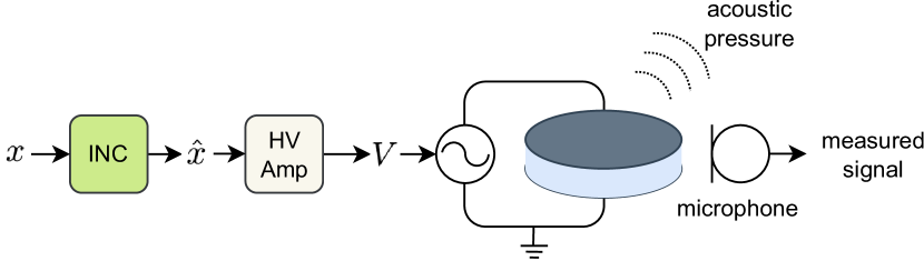
(a) Illustration of the measurement

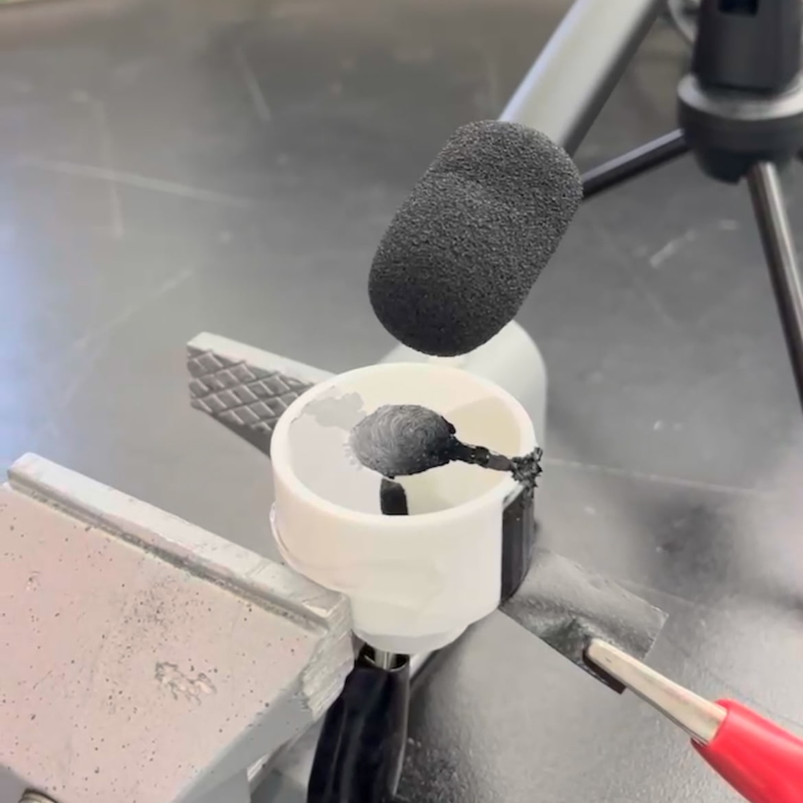
(b) DEA Sample

Figure 10: DEA measurement equipment setup.

We use 3M^™ VHB^™ Tape 4910 as the elastomer of our DEA. The elastomer is pre-stretched biaxially by a factor of 3.0, to be hung on a plastic frame. We apply carbon grease on the elastomer to manufacture the dielectric elastomer. So the VHB tape is sandwiched by the carbon grease electrode. Regarding stability and Assumption 3, the electrodes are applied to only a portion of the center of the elastomer. We amplify the voltage signal by a factor of 1000 to actuate the DEA. The actuated sound is picked up using a Behringer™ ECM8000 microphone. Figure 10 shows a photo of part of the experimental setup.

References

- Pelrine et al. [2000] R. Pelrine, R. Kornbluh, Q. Pei, J. Joseph, High-speed electrically actuated elastomers with strain greater than 100%, Science 287 (2000) 836–839.
- Huang et al. [2012] J. Huang, T. Li, C. Chiang Foo, J. Zhu, D. R. Clarke, Z. Suo, Giant, voltage-actuated deformation of a dielectric elastomer under dead load, Applied Physics Letters 100 (2012).
- Rogers [2013] J. A. Rogers, A clear advance in soft actuators, Science 341 (2013) 968–969.
- Kim et al. [2019] D. Y. Kim, S. Choi, H. Cho, J.-Y. Sun, Electroactive soft photonic devices for the synesthetic perception of color and sound, Advanced Materials 31 (2019) 1804080.
- Kornbluh et al. [2002] R. Kornbluh, R. Pelrine, Q. Pei, Dielectric elastomer produces strain of 380%, EAP Newsletter 2 (2002) 10–11.
- Keplinger et al. [2012] C. Keplinger, T. Li, R. Baumgartner, Z. Suo, S. Bauer, Harnessing snap-through instability in soft dielectrics to achieve giant voltage-triggered deformation, Soft Matter 8 (2012) 285–288.
- Li et al. [2018] Y. Li, I. Oh, J. Chen, H. Zhang, Y. Hu, Nonlinear dynamic analysis and active control of visco-hyperelastic dielectric elastomer membrane, International Journal of Solids and Structures 152 (2018) 28–38.
- Kanan and Kaliske [2021] A. Kanan, M. Kaliske, On the computational modelling of nonlinear electro-elasticity in heterogeneous bodies at finite deformations, Mechanics of Soft Materials 3 (2021) 1–19.
- Kashyap et al. [2020] K. Kashyap, A. K. Sharma, M. M. Joglekar, Nonlinear dynamic analysis of aniso-visco-hyperelastic dielectric elastomer actuators, Smart Materials and Structures 29 (2020) 055014.
- Kim et al. [2019] D. Y. Kim, M.-J. Kim, G. Sung, J.-Y. Sun, Stretchable and reflective displays: materials, technologies and strategies, Nano Convergence 6 (2019) 1–24.
- Heydt et al. [1998] R. Heydt, R. Kornbluh, R. Pelrine, V. Mason, Design and performance of an electrostrictive-polymer-film acoustic actuator, Journal of Sound and Vibration 215 (1998) 297–311.
- Heydt et al. [2000] R. Heydt, R. Pelrine, J. Joseph, J. Eckerle, R. Kornbluh, Acoustical performance of an electrostrictive polymer film loudspeaker, The Journal of the Acoustical Society of America 107 (2000) 833–839.
- Carpi et al. [2011] F. Carpi, D. De Rossi, R. Kornbluh, R. E. Pelrine, P. Sommer-Larsen, Dielectric elastomers as electromechanical transducers: Fundamentals, materials, devices, models and applications of an emerging electroactive polymer technology, Elsevier, 2011.
- Hines et al. [2017] L. Hines, K. Petersen, G. Z. Lum, M. Sitti, Soft actuators for small-scale robotics, Advanced materials 29 (2017) 1603483.
- Petralia and Wood [2010] M. T. Petralia, R. J. Wood, Fabrication and analysis of dielectric-elastomer minimum-energy structures for highly-deformable soft robotic systems, in: 2010 IEEE/RSJ International Conference on Intelligent Robots and Systems, IEEE, 2010, pp. 2357–2363.
- Anderson et al. [2012] I. A. Anderson, T. A. Gisby, T. G. McKay, B. M. O’Brien, E. P. Calius, Multi-functional dielectric elastomer artificial muscles for soft and smart machines, Journal of applied physics 112 (2012) 041101.
- Herold et al. [2011] S. Herold, W. Kaal, T. Melz, Dielectric elastomers for active vibration control applications, in: Electroactive Polymer Actuators and Devices (EAPAD) 2011, volume 7976, International Society for Optics and Photonics, 2011, p. 79761I.
- Li et al. [2012] T. Li, S. Qu, W. Yang, Electromechanical and dynamic analyses of tunable dielectric elastomer resonator, International Journal of Solids and Structures 49 (2012) 3754–3761.
- Lu et al. [2015a] Z. Lu, Y. Cui, M. Debiasi, Z. Zhao, A tunable dielectric elastomer acoustic absorber, Acta Acustica united with Acustica 101 (2015a) 863–866.
- Lu et al. [2015b] Z. Lu, H. Godaba, Y. Cui, C. C. Foo, M. Debiasi, J. Zhu, An electronically tunable duct silencer using dielectric elastomer actuators, The Journal of the Acoustical Society of America 138 (2015b) EL236–EL241.
- Bortot and Shmuel [2017] E. Bortot, G. Shmuel, Tuning sound with soft dielectrics, Smart Materials and Structures 26 (2017) 045028.
- Huang et al. [2016] Z.-l. Huang, X.-l. Jin, R.-h. Ruan, W.-q. Zhu, Typical dielectric elastomer structures: dynamics and application in structural vibration control, Journal of Zhejiang University-Science A 17 (2016) 335–352.
- Tan et al. [2003] C.-T. Tan, B. C. Moore, N. Zacharov, The effect of nonlinear distortion on the perceived quality of music and speech signals, Journal of the Audio Engineering Society 51 (2003) 1012–1031.
- Ogden [1997] R. W. Ogden, Non-linear elastic deformations, Courier Corporation, 1997.
- Gent [1996] A. N. Gent, A new constitutive relation for rubber, Rubber chemistry and technology 69 (1996) 59–61.
- Pelrine et al. [1998] R. E. Pelrine, R. D. Kornbluh, J. P. Joseph, Electrostriction of polymer dielectrics with compliant electrodes as a means of actuation, Sensors and Actuators A: Physical 64 (1998) 77–85.
- Huang et al. [2021] J. Huang, X. Feng, S. Chen, Y. Shen, Analysis of total harmonic distortion of miniature loudspeakers used in mobile phones considering nonlinear acoustic damping, The Journal of the Acoustical Society of America 149 (2021) 1579–1588.
- Albach and Lerch [2013] T. S. Albach, R. Lerch, Magnetostrictive microelectromechanical loudspeaker, The Journal of the Acoustical Society of America 134 (2013) 4372–4380.
- Goulbourne et al. [2005] N. Goulbourne, E. Mockensturm, M. Frecker, A nonlinear model for dielectric elastomer membranes, Journal of Applied Mechanics 72 (2005) 899–906.
- Ogden [1972] R. W. Ogden, Large deformation isotropic elasticity–on the correlation of theory and experiment for incompressible rubberlike solids, Proceedings of the Royal Society of London. A. Mathematical and Physical Sciences 326 (1972) 565–584.
- Mooney [1940] M. Mooney, A theory of large elastic deformation, Journal of applied physics 11 (1940) 582–592.
- Rivlin [1948] R. S. Rivlin, Large elastic deformations of isotropic materials iv. further developments of the general theory, Philosophical transactions of the royal society of London. Series A, Mathematical and physical sciences 241 (1948) 379–397.
- Treloar [1943] L. Treloar, The elasticity of a network of long-chain molecules—ii, Transactions of the Faraday Society 39 (1943) 241–246.
- Xu et al. [2012] B.-X. Xu, R. Mueller, A. Theis, M. Klassen, D. Gross, Dynamic analysis of dielectric elastomer actuators, Applied Physics Letters 100 (2012) 112903.
- Hochradel et al. [2012] K. Hochradel, S. Rupitsch, A. Sutor, R. Lerch, D. Vu, P. Steinmann, Dynamic performance of dielectric elastomers utilized as acoustic actuators, Applied Physics A 107 (2012) 531–538.
- Heidari et al. [2020] H. Heidari, A. Alibakhshi, H. R. Azarboni, Chaotic motion of a parametrically excited dielectric elastomer, International Journal of Applied Mechanics 12 (2020) 2050033.
- Sheng et al. [2013] J. Sheng, H. Chen, L. Liu, J. Zhang, Y. Wang, S. Jia, Dynamic electromechanical performance of viscoelastic dielectric elastomers, Journal of Applied Physics 114 (2013) 134101.
- Sheng et al. [2014] J. Sheng, H. Chen, B. Li, Y. Wang, Nonlinear dynamic characteristics of a dielectric elastomer membrane undergoing in-plane deformation, Smart Materials and Structures 23 (2014) 045010.
- Hiruta et al. [2021] T. Hiruta, N. Hosoya, S. Maeda, I. Kajiwara, Experimental validation of vibration control in membrane structures using dielectric elastomer actuators in a vacuum environment, International Journal of Mechanical Sciences 191 (2021) 106049.
- Zhang et al. [2023] Y. Zhang, J. Wu, P. Huang, C.-Y. Su, Y. Wang, Inverse dynamics modelling and tracking control of conical dielectric elastomer actuator based on gru neural network, Engineering Applications of Artificial Intelligence 118 (2023) 105668.
- Xiao et al. [2020] H. Xiao, J. Wu, W. Ye, Y. Wang, Dynamic modeling for dielectric elastomer actuators based on lstm deep neural network, in: 2020 5th international conference on advanced robotics and mechatronics (ICARM), IEEE, 2020, pp. 119–124.
- Li et al. [2019] L. Li, J. Li, L. Qin, J. Cao, M. S. Kankanhalli, J. Zhu, Deep reinforcement learning in soft viscoelastic actuator of dielectric elastomer, IEEE Robotics and Automation Letters 4 (2019) 2094–2100.
- Hornik et al. [1989] K. Hornik, M. Stinchcombe, H. White, et al., Multilayer feedforward networks are universal approximators., Neural networks 2 (1989) 359–366.
- Hornik [1991] K. Hornik, Approximation capabilities of multilayer feedforward networks, Neural networks 4 (1991) 251–257.
- Leshno et al. [1993] M. Leshno, V. Y. Lin, A. Pinkus, S. Schocken, Multilayer feedforward networks with a nonpolynomial activation function can approximate any function, Neural networks 6 (1993) 861–867.
- Lagaris et al. [1998] I. E. Lagaris, A. Likas, D. I. Fotiadis, Artificial neural networks for solving ordinary and partial differential equations, IEEE transactions on neural networks 9 (1998) 987–1000.
- Chen et al. [2018] R. T. Chen, Y. Rubanova, J. Bettencourt, D. K. Duvenaud, Neural ordinary differential equations, Advances in neural information processing systems 31 (2018).
- Raissi et al. [2019] M. Raissi, P. Perdikaris, G. E. Karniadakis, Physics-informed neural networks: A deep learning framework for solving forward and inverse problems involving nonlinear partial differential equations, Journal of Computational physics 378 (2019) 686–707.
- Li et al. [2021] Z. Li, N. B. Kovachki, K. Azizzadenesheli, B. liu, K. Bhattacharya, A. Stuart, A. Anandkumar, Fourier neural operator for parametric partial differential equations, in: International Conference on Learning Representations, 2021. URL: openreview.net/forum?id=c8P9NQVtmnO.
- Gupta et al. [2021] G. Gupta, X. Xiao, P. Bogdan, Multiwavelet-based operator learning for differential equations, Advances in neural information processing systems 34 (2021) 24048–24062.
- Lee et al. [2018] J. Lee, S. Lee, D. You, Deep learning approach in multi-scale prediction of turbulent mixing-layer, arXiv preprint arXiv:1809.07021 (2018).
- Lee and You [2019] S. Lee, D. You, Data-driven prediction of unsteady flow over a circular cylinder using deep learning, Journal of Fluid Mechanics 879 (2019) 217–254.
- Lee et al. [2023] J. W. Lee, M. J. Choi, K. Lee, String sound synthesizer on gpu-accelerated finite difference scheme, arXiv preprint arXiv:2311.18505 (2023).
- Taghizadeh and Darijani [2018] D. Taghizadeh, H. Darijani, Mechanical behavior modeling of hyperelastic transversely isotropic materials based on a new polyconvex strain energy function, International Journal of Applied Mechanics 10 (2018) 1850104.
- Arruda and Boyce [1993] E. M. Arruda, M. C. Boyce, A three-dimensional constitutive model for the large stretch behavior of rubber elastic materials, Journal of the Mechanics and Physics of Solids 41 (1993) 389–412.
- Jia et al. [2019] K. Jia, T. Lu, T. Wang, Deformation study of an in-plane oscillating dielectric elastomer actuator having complex modes, Journal of Sound and Vibration 463 (2019) 114940.
- Zhu et al. [2010] J. Zhu, S. Cai, Z. Suo, Resonant behavior of a membrane of a dielectric elastomer, International Journal of Solids and Structures 47 (2010) 3254–3262.
- Garnell et al. [2019] E. Garnell, C. Rouby, O. Doaré, Dynamics and sound radiation of a dielectric elastomer membrane, Journal of Sound and Vibration 459 (2019) 114836.
- Zhang et al. [2016] J. Zhang, J. Zhao, H. Chen, D. Li, Dynamic analyses of viscoelastic dielectric elastomers incorporating viscous damping effect, Smart Materials and Structures 26 (2016) 015010.
- Zhang et al. [2015] J. Zhang, L. Tang, B. Li, Y. Wang, H. Chen, Modeling of the dynamic characteristic of viscoelastic dielectric elastomer actuators subject to different conditions of mechanical load, Journal of Applied Physics 117 (2015).
- Zhou et al. [2016] J. Zhou, L. Jiang, R. E. Khayat, Dynamic analysis of a tunable viscoelastic dielectric elastomer oscillator under external excitation, Smart Materials and Structures 25 (2016) 025005.
- Eder-Goy et al. [2017] D. Eder-Goy, Y. Zhao, B.-X. Xu, Dynamic pull-in instability of a prestretched viscous dielectric elastomer under electric loading, Acta Mechanica 228 (2017) 4293–4307.
- Miyamoto et al. [1988] H. Miyamoto, M. Kawato, T. Setoyama, R. Suzuki, Feedback-error-learning neural network for trajectory control of a robotic manipulator, Neural networks 1 (1988) 251–265.
- Zou and Gu [2018] J. Zou, G. Gu, High-precision tracking control of a soft dielectric elastomer actuator with inverse viscoelastic hysteresis compensation, IEEE/ASME Transactions on Mechatronics 24 (2018) 36–44.
- Zou and Gu [2019] J. Zou, G. Gu, Feedforward control of the rate-dependent viscoelastic hysteresis nonlinearity in dielectric elastomer actuators, IEEE Robotics and Automation Letters 4 (2019) 2340–2347.
- Jastrze et al. [2009] R. P. Jastrze, R. Pöllänen, et al., Compensation of nonlinearities in active magnetic bearings with variable force bias for zero-and reduced-bias operation, Mechatronics 19 (2009) 629–638.
- Skricka and Markert [2002] N. Skricka, R. Markert, Improvements in the integration of active magnetic bearings, Control Engineering Practice 10 (2002) 917–922.
- Le Brun [1979] M. Le Brun, Digital waveshaping synthesis, Journal of the Audio Engineering Society 27 (1979) 250–266.
- Arfib [1978] D. Arfib, Digital synthesis of complex spectra by means of multiplication of non linear distorted sine waves, in: Audio Engineering Society Convention 59, Audio Engineering Society, 1978.
- Dodge and Jerse [1985] C. Dodge, T. A. Jerse, Computer music: synthesis, composition, and performance, Macmillan Library Reference, 1985.
- Roads [1979] C. Roads, A tutorial on non-linear distortion or waveshaping synthesis, Computer Music Journal (1979) 29–34.
- Hayes et al. [2021] B. Hayes, C. Saitis, G. Fazekas, Neural waveshaping synthesis, in: Proceedings of the 22nd International Society for Music Information Retrieval Conference, ISMIR, 2021, pp. 254–261.
- Serra and Smith [1990] X. Serra, J. Smith, Spectral modeling synthesis: A sound analysis/synthesis system based on a deterministic plus stochastic decomposition, Computer Music Journal 14 (1990) 12–24.
- Engel et al. [2020] J. Engel, L. H. Hantrakul, C. Gu, A. Roberts, Ddsp: Differentiable digital signal processing, in: International Conference on Learning Representations, 2020. URL: openreview.net/forum?id=B1x1ma4tDr.
- Wang et al. [2016] F. Wang, T. Lu, T. Wang, Nonlinear vibration of dielectric elastomer incorporating strain stiffening, International Journal of Solids and Structures 87 (2016) 70–80.
- Alibakhshi and Heidari [2019] A. Alibakhshi, H. Heidari, Analytical approximation solutions of a dielectric elastomer balloon using the multiple scales method, European Journal of Mechanics-A/Solids 74 (2019) 485–496.
- Virtanen et al. [2020] P. Virtanen, R. Gommers, T. E. Oliphant, M. Haberland, T. Reddy, D. Cournapeau, E. Burovski, P. Peterson, W. Weckesser, J. Bright, S. J. van der Walt, M. Brett, J. Wilson, K. J. Millman, N. Mayorov, A. R. J. Nelson, E. Jones, R. Kern, E. Larson, C. J. Carey, İ. Polat, Y. Feng, E. W. Moore, J. VanderPlas, D. Laxalde, J. Perktold, R. Cimrman, I. Henriksen, E. A. Quintero, C. R. Harris, A. M. Archibald, A. H. Ribeiro, F. Pedregosa, P. van Mulbregt, SciPy 1.0 Contributors, SciPy 1.0: Fundamental Algorithms for Scientific Computing in Python, Nature Methods 17 (2020) 261–272. doi:10.1038/s41592-019-0686-2.
- Dormand and Prince [1980] J. R. Dormand, P. J. Prince, A family of embedded runge-kutta formulae, Journal of computational and applied mathematics 6 (1980) 19–26.
- Bozlar et al. [2012] M. Bozlar, C. Punckt, S. Korkut, J. Zhu, C. Chiang Foo, Z. Suo, I. A. Aksay, Dielectric elastomer actuators with elastomeric electrodes, Applied physics letters 101 (2012).
- Vu-Cong et al. [2012] T. Vu-Cong, C. Jean-Mistral, A. Sylvestre, Impact of the nature of the compliant electrodes on the dielectric constant of acrylic and silicone electroactive polymers, Smart Materials and Structures 21 (2012) 105036.
- Horn [1983] M. K. Horn, Fourth-and fifth-order, scaled rungs–kutta algorithms for treating dense output, SIAM Journal on Numerical Analysis 20 (1983) 558–568.
- Shampine [1985] L. F. Shampine, Interpolation for runge–kutta methods, SIAM journal on Numerical Analysis 22 (1985) 1014–1027.
- Shampine [1986] L. F. Shampine, Some practical runge-kutta formulas, Mathematics of computation 46 (1986) 135–150.
- Kingma and Ba [2015] D. Kingma, J. Ba, Adam: A method for stochastic optimization, in: International Conference on Learning Representations (ICLR), San Diego, CA, USA, 2015.