Confinement Bubble Wall Velocity via Quasiparticle Determination

Abstract

Lattice simulations reveal that the deconfinement-confinement (D-C) phase transition (PT) of the hot pure $SU(N>2)$ Yang-Mills system is first order. This system can be described by a pool of quasigluons moving in the Polyakov loop background, and in this picture, we establish an effective distribution function for quasigluons, which encodes interactions among quasigluons and in particular the confinement effect. With it, we made the first attempt to calculate the confinement bubble wall velocity $v_{w}$ at the microscopical level, and we obtained a small velocity $v_{w}\sim 0.04$ using two different approaches, which is qualitatively consistent with others results like holography.

Cosmic PT for vacuum and substance In 1937, Landau proposed an approach to study continuous PT characterized by the spontaneous breaking of symmetry $G$. The key is to select an appropriate order parameter $\phi$ and construct an $G$-invariant Landau free energy ${\cal L}[\phi,T]$, encoding the order of PTs and as well the behavior of relevant thermodynamic properties near the critical point. If the transition for the matter system is first order, the non-equilibrium evolution for phase conversion may be simplified to be the picture of bubble nucleation and growth Langer:1969bc ; Csernai:1992tj . This coarse-grained theory is a combination of classical nucleation theory, dealing with liquid-gas PT, and the Ginzburg-Landau free energy. The order parameter is chosen to be the collective variable, the deviation of the energy density from its equilibrium value.

When Landau’s idea is applied to describe cosmic PTs, a big difference arises: the order parameter field here is a given “matter” field whose VEV labels the vacuum, such as inflation field, Higgs field, etc., not just a macroscopic quantity selected in the thermodynamic matter system such as density or magnetization. The PT here is not related to changes in the structure of matter, but rather to changes in the vacuum of the field system, known as vacuum PT. It can proceed due to purely quantum fluctuations, and then first order phase conversion is through the vacuum decay developed by Coleman Coleman:1977py and Callan Callan:1977pt . Later, it is generalized to finite temperature by Affleck Affleck:1980ac and Linde Linde:1981zj . In this context, the order parameter does not necessarily transform under some symmetry, although most studies begin with a symmetry.

Electroweak-like PT (EWPT) is a well-known example to illustrate the difference. The Landau free energy in the cosmological field system is usually not guessed at the mean field level and can be calculated perturbatively. It generally takes the form $V_{eff}(\phi)=V_{0}(\phi)+V_{T}(\phi)$ with $V_{0}$ the zero temperature potential and $V_{T}(\phi)$ due to the plasma matter gas made of quarks and leptons etc, interacting with $\phi$. The resulting PT makes the universe transit from the EW symmetric vacuum to the broken one, but the plasma particles simply become heavier in the new vacuum without structural changes.

D-C PT: non-perturbative gluonic vacuum reconstruction However, for the QCD-like system showing asymptotic freedom and confinement, it becomes different and much more complicated to study its presumptive PT from the qausigluon phase (or Debye screening phase) to the glueball (confinement) phase Polyakov:1978vu ; Susskind:1979up ; Olive:1980dy ; Witten:1984rs .

No obvious order parameter is present. The modulus of the expected value of the gauge invariant Polyakov loop (PL) $\ell(\vec{x})\equiv\frac{1}{N}{\rm tr}_{c}{\cal P}\exp{ig\int_{0}^{\beta}d\tau A_{4}(\vec{x},\tau)}$, which may be related to the free energy of a single static quark $Q$ via $\Phi=|\langle\ell(\vec{x})\rangle|\propto e^{-F_{Q}/T}$ McLerran:1981pb . It can be interpreted as the probability to observe a single quark in the gluonic plasma, which will be supported in a different way later. Then, $\Phi\to 0$ implies an infinite $F_{Q}$, signaling color confinment. On the contrary, $\Phi\neq 0$ means a finite $F_{Q}$ thus deconfinement. Moreover, PL is charged under the global center $Z_{N}\subset SU(N)$, and thus $\Phi$ is widely used as the order parameter for D-C PT. However, the presence of dynamical fermions with nonzero $N-$ality violates $Z_{N}$, rendering $\Phi$ merely a pseudo order parameter.

PL is a nonlocal operator of the fundamental field $A_{0}$, which can not be gauged away at finite $T$. Then, $A_{0}$ are nothing but real scalars in the adjoint representation of $SU(N)$, and its transition from the deconfinement vacuum with a vanishingly small condensate to the confinement vacuum with a large condensate drives the transition of PL . In this sense, D-C PT is a vacuum PT associated with the spontaneously breaking of $SU(N)$.

Quasiparticle moving in the PL background We need a model to describe the system at $T_{c}^{+}$, where the non-perturbative effect becomes significant. The weakly interacting quasigluon picture with $T$-dependent mass assumed to “absorb” the dominant gluon interaction, can successfully account for thermodynamics down to $T_{c}$ Goloviznin:1992ws ; Peshier:1995ty . But this statistical model does not address PT. Alternatively, Pisarski treats the QGP as a condensate of PL Pisarski:2000eq , without particle excitations at all. A well-designed Landau free energy works well from a few $T_{c}$ down to $T_{c}$, including the D-C PT. Quasigluons moving on the PL background is a hybrid approach Meisinger:2003id ; Ruggieri:2012ny ; Sasaki:2012bi ; Alba:2014lda ; Islam:2021qwh . Following the spirit of quasi particles, it implies a possible perturbative field picture of hot PYM at $T_{c}^{+}$: one may introduce a $T$-dependent gluon mass parameter to the original PYM Lagrangian, “absorbing” the main nonperturbative interactions, and then the Landau free energy can be perturbatively calculated Kang:2022jbg .

The model in Ref. Kang:2022jbg is a generalization to the massive PYM model Reinosa:2014ooa to the case with a temperature dependent quasigluon mass $M_{g}(T)$,

$$\mathcal{L}=-\frac{1}{2g^{2}}{\rm tr}(F_{\mu\nu}F^{\mu\nu})+\bar{D}_{\mu}\bar{c}^{a}D^{\mu}c^{a}$$ (1)

$$+ih^{a}\bar{D}_{\mu}\hat{A}^{\mu,a}+\frac{1}{2}M^{2}_{g}(T)\hat{A}^{a}_{\mu}\hat{A}^{a,\mu},$$

with $c,\bar{c}$ and $h$ the Ghost fields, real Nakanishi-Lautrup field, respectively. $A_{\mu}$ is decomposed into a background $\bar{A}_{\mu}=\bar{A}_{0}^{i}H^{i}\delta_{0\mu}$ ($H_{i}$ the Cartan generators) plus massive fluctuations $\hat{A}_{\mu}$. In the Landau-DeWitt gauge $\bar{D}_{\mu}\hat{A}^{\mu}=0$ with $\bar{D}_{\mu}^{ab}=\partial_{\mu}\delta^{ab}+f^{acb}\bar{A}^{c}_{\mu}$, we integrate out the fluctuations to obtain the potential ${V}_{eff}=\frac{1}{V}\log Z$ with

$$\begin{split}\log Z=VT\Bigg{[}3\int\frac{d^{3}p}{(2\pi)^{3}}\log\det\left(1-\hat{L}_{A}e^{-\frac{E_{g}}{T}}\right)\\ -\int\frac{d^{3}p}{(2\pi)^{3}}\log\det\left(1-\hat{L}_{A}e^{-\frac{|\vec{p}|}{T}}\right)\Bigg{]},\end{split}$$ (2)

where $E_{g}=\sqrt{|\vec{p}|^{2}+M_{g}^{2}}$ and $\hat{L}_{A}$ is the thermal Polyakov loop in the adjoint representation. One may parameterize $\bar{A}_{4}=i\bar{A}_{0}=\frac{2\pi}{g\beta}{\rm diag}(q_{1},...,q_{N})$ with $\sum_{i-1}^{N}q_{i}=0$ for a real PL. Then, $\hat{L}_{A}={\rm diag}[e^{\beta\mu_{1}},e^{\beta\mu_{2}},...,e^{\beta\mu_{N^{2}-1}}]$, where $\mu_{a}$ picks one value of $\{i2\pi q_{ij}/\beta\}$ with $q_{ij}\equiv q_{i}-q_{j}$. We take the equal eigenvalue distribution assumption $q_{ij}=\frac{i-j}{N}s$ Roberge:1986mm ; Dumitru:2010mj ; Kang:2022jbg . For example, in $SU(3)$ and $SU(4)$ they are respectively given by:

$$\begin{split}\frac{\beta}{2\pi}\mu_{a}=&\{0,i\frac{s}{3},-i\frac{s}{3},i\frac{2s}{3},-i\frac{2s}{3},i\frac{s}{3},-i\frac{s}{3},0\},\\ \frac{\beta}{2\pi}\mu_{a}=&\{0,i\frac{s}{4},-i\frac{s}{4},i\frac{s}{2},-i\frac{s}{2},i\frac{s}{4},-i\frac{s}{4},0,\\ &i\frac{s}{4},-i\frac{s}{4},i\frac{s}{2},-i\frac{s}{2},i\frac{3s}{4},-i\frac{3s}{4},0\}.\end{split}$$ (3)

They will be interpreted as the imaginary chemical potential.

Near $T_{c}$, the increasing quasigluon mass leads to the ghost contribution becomes relatively important. In this sense, it is a manifestation of non-perturbation effects in the infrared region, which destabilizes the perturbation deconfinement vacuum at $s_{d}=0$, to arrive the confinement vacuum at $s_{c}=1$ via first order PT.

As we claimed before, the D-C PT may be treated as a vacuum PT. As for the transition of quasigluons to the confinement phase, it is somewhat similar to EWPT. As a Landau approach, the above model does not provide the microscopic mechanism for color confinement, but in the following, we will see that statistically it is attributed to the imaginary potential $\mu$. Then, we can claim that quasigluons in two different phases simply have different $\mu$, a change also encoded in the dispersion relation of quasigluons.

Effective statistical description of non-ideal quasi-gluon Different from the traditional quasiparticle model which is a statistical model, simply treating the QGP as a pool of “ideal” quasiparticle gas with temperate varying mass , the pressure calculated in the field theory ${\cal P}=-{\cal V}_{eff}$ includes the contribution of ghost and as well the background field PL. Note that viewing from statistics, it corresponds to the pressure of the ensemble without bulk motion, denoted as ${\cal P}$ exclusively. Let us rewrite it in a more familiar form:

$${\cal P}=\sum_{a=1}^{N^{2}-1}\int\frac{d^{3}\vec{p}}{(2\pi)^{3}}\frac{1}{e^{\beta(E-\mu_{a})}-1}\frac{|\vec{p}|^{2}}{E}-$$ (4)

$$\frac{1}{3}\sum_{a=1}^{N^{2}-1}\int\frac{d^{3}\vec{p}}{(2\pi)^{3}}\frac{1}{e^{\beta(|\vec{p}|-\mu_{a})}-1}\frac{|\vec{p}|^{2}}{|\vec{p}|},$$

It resembles a mixture of ideal gas of massive gauge bosons with three degrees of freedom, plus one massless “ghost”, thus carrying a minus sign from its unphysical role in the FP procedure. Note that the conventional Bose-Einstein distribution functions are twisted by the imaginary chemical potential $\mu_{a}$, and thus become complex $f_{a}(E,\mu_{a})$. A similar result is known before such as in Ref. Hidaka:2008dr , but it is obtained via a direct generalization of ordinary distribution functions based on the modified dispersion relation as discussed in Eq. (10).

Instead of mass, here the background field enters the imaginary chemical potential of the quasigluons and results in statistical confinement. One can calculate the corresponding number density using $f_{a}$ ($a$ summed over all color indices) in two phases, to find that there is a significant suppression in the confinement phase. This is a surprising result, because so far we have not yet forced quasigluons to form glueballs at $T_{c}^{+}$, the degree of freedom not included in our microscopic approach. A natural conjecture is that the quasigluons have been converted to glueballs during D-C PT. There is an interesting interpretation in the dynamical quasigluon scenario Cassing:2007yg : the force between quasigluons derived from the mean field is van der Waals like, and it becomes attractive as the quasigluon density drops below some critical value. Whether this mechanism can work here still needs further research, but we can also consider an alternative solution: the gluons may convert to vacuum condensate rather than to glueballs, which are produced via the wall oscillation after bubble collision. Anyway, for the purpose of calculating wall velocity, it is reasonable to speculate that it only plays a minor role, as lattice data tells us that the confinement phase is almost pressureless.

Fluid pressure on the wall: from Micro to Statistical Due to the driving force of the two-phase vacuum pressure difference $\Delta P=\Delta V_{eff}$, overcritical bubbles will maintain accelerated expansion in the fluid until the reaction force of the fluid increases to $F_{w}(v_{w})/A=\Delta P$, resulting in a balanced force on the bubble wall and reaching a steady state. For EWPT, it is clear that the zero temperature scalar potential difference plays the role of driving force, and mass increasing when plasma particles cross the wall exerts an effective friction on the wall, impeding the bubble expansion. But in the D-C PT, we do not have a tree level potential and then the steady equation is simply reduced to $F_{w}(v_{w})/A=0$.

In principle, $F_{w}(v_{w})$ can be calculated from a microscopic perspective. We consider the sufficiently large bubbles in the big plane limit, moving along the $-z$ axis. In the wall frame, suppose a particle passing through a wall exerts a force $F_{sp}(z)$ on the wall, then the pressure acting on the bubble wall is the total force per unit area $\frac{F_{w}}{A}=\int dz\int\frac{d^{3}\vec{p}}{(2\pi)^{3}}F_{sp}(z)f(p,z)$ Moore:2000wx . However, here $F_{sp}$ is hard to find, and thus we bypass this issue through the Boltzmann equation Konstandin:2014zta ; Hindmarsh:2020hop

$$(p^{\mu}\partial_{\mu}+mF^{\mu}\partial_{p^{\mu}})\theta(p^{0})\delta(p^{2}+m^{2})f=C[f]$$ (5)

with $F^{\mu}$ the external force acting on the particle.

First, let us multiply $p^{\nu}$ on both sides of Eq. (5) and integrate over $\vec{p}$, to find that the collision term vanishes as a result of energy momentum conservation in local thermal equilibrium. Further integrating over $p_{0}$, assuming that $F^{\mu}$ is momentum independent, we get

$$\partial_{\mu}\int\frac{d^{3}\vec{p}}{(2\pi)^{3}}\frac{p^{\nu}p^{\mu}}{E}f\equiv\partial_{\mu}T_{f}^{\mu\nu}=\int\frac{d^{3}\vec{p}}{(2\pi)^{3}}mF^{\mu}\frac{f}{E}.$$ (6)

It gives the evolution of the energy tensor of the fluid system $\partial_{\mu}T_{f}^{\mu\nu}\neq 0$, due to the interaction between fluid and wall. To study the steady bubble expansion, it is convenient to use Eq. (6) in the bubble wall frame where the time variable becomes irrelevant. Setting $\mu=z$ and using $F^{z}(z)=\frac{dp^{z}}{d\tau}=\frac{dt}{d\tau}\frac{dp^{z}}{dt}=\frac{E}{m}F_{sp}(z)$, Eq. (6) turns out to be $\frac{d}{dz}\int\frac{d^{3}\vec{p}}{(2\pi)^{3}}\frac{p_{z}^{2}}{E}f_{w}(p,z)=\int\frac{d^{3}\vec{p}}{(2\pi)^{3}}F_{sp}(z)f_{w}(p,z)$, with $f_{w}$ the distribution function in the bubble wall frame. Integrate it over $z$ we finally arrive

$$\Delta T^{zz}_{f}=\Delta\left[\int\frac{d^{3}\vec{p}}{(2\pi)^{3}}\frac{p_{z}^{2}}{E}f_{w}(p,z)\right]_{z=-\infty}^{z=\infty}=\frac{f_{w}}{A}.$$ (7)

It establishes the relation between pressure on the wall and the discontinuous of $T_{f}^{zz}$, determined by the steady-state distributions function on both sides. That is to say, one can use this statistical formula to compute the pressure without knowing $F_{sp}$, as long as we can find the distribution functions in the two phases far away from the wall. Actually, this is not a novel result, and it has been used before as the direct definition of pressure in the bubble frame BarrosoMancha:2020fay . Here we derived it from BE. In the following, we will use this formula to study the bubble wall velocity in the D-C PT.

Before proceeding, we would like to make a comment. An important assumption we should make is that the fluid inside (at least sufficiently far from the wall) the bubble has been thermalized, as is reasonable for slow-moving bubbles and fast scattering of the particle composition of the fluid. This is just the situation here. Otherwise, nonequilibrium effects will play a significant role that can not be addressed by the above approach and we may need to solve the BE just like in EWPT DeCurtis:2022hlx ; Laurent:2022jrs ; DeCurtis:2022llw .

Steady confinement bubble wall velocity The ordinary fluid approach Steinhardt:1981ct ; Espinosa:2010hh ; Ai:2021kak ; LiLi:2023dlc ; Wang:2023lam ; Ai:2024shx , which expresses $T^{zz}_{f}$ in terms of the thermodynamic macroscopic quantities, is developed to deal with EWPT, and does not apply here, owing to the fact the quasigluons significantly deviate from the ideal gas. But Eq. (7) is based on the statistic approach, thus in principle applying to any fluid. Here, the crucial distribution function $f_{w}$ can be obtained by boosting the effective distribution functions (at infinity) in the fluid rest frame to the bubble frame

$$f_{w,a}(v_{w},p,z)=1/(\exp\beta[\gamma(E-v_{w}p_{z}+\mu_{a}(z))]-1),$$ (8)

where the bubble expansion velocity $v_{w}$ enters.

In this frame, the steady bubble expansion means the static equation $F_{w}/A=\Delta T^{zz}_{f}=0$. Substituting Eq. (8) into the static equation, we get the pressure acting on the wall, $P_{w}=P(s_{c})-P(s_{d})$. Note that the distribution functions with an imaginary part seem to be unphysical, however, in various physical quantities, their integral in the momentum space leads to real values by virtue of the exact cancelation between the $\mu_{i}$ and $-\mu_{i}$ terms. We have computed $P_{w}(v_{w})$ for $N=3-6$ and plot them in the left panel of Fig. 1. From this figure, it is clearly seen that, starting from a small initial velocity, the (decreasing) total force continues to accelerate the expansion of the wall until the wall velocity increases to a certain terminal value $v_{w}$. One can find that the terminal velocity for different $N$ takes a similar value, $v_{w}\approx 0.04$, which is qualitatively consistent with the previous results from the fluid or holography approach Kajantie:1986hq ; Ignatius:1993qn ; LiLi:2023dlc ; Wang:2023lam ; Bea:2021zsu ; Bigazzi:2021ucw ; Janik:2022wsx .

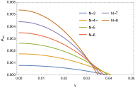
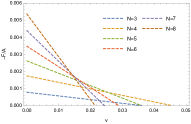
Figure 1: Steady bubble wall velocity from the statistic approach (left) and the microscopic approach (right).

Back to Micro There is a more widely used formula to calculate the microscopic friction exerted by plasma particles on the moving wall, not based on the specific external force, but on momentum transfer Arnold:1993wc ; Bodeker:2009qy ; Bodeker:2017cim ; Azatov:2020ufh ; Gouttenoire:2021kjv :

$$\frac{dF_{w}}{A}=\frac{d^{3}\vec{p}}{(2\pi)^{3}}v_{z}f_{w}(p)\Delta p_{z}P(\Delta p_{z})$$ (9)

where $\frac{d^{3}\vec{p}}{(2\pi)^{3}}v_{z}f_{w}(p)$ is the flux of particle with velocity $v_{z}=p_{z}/\sqrt{|\vec{p}|^{2}+M_{g}^{2}}$, and $P(\Delta p_{z})$ is the probability for a quasigluon and ghost passing through the wall and transferring momentum $\Delta p_{z}$ to it.

In our approach, the momentum transfer is induced by the change of $\mu_{a}$ in two phases , and can be estimated via the modified dispersion relation on the background:

$$\begin{split}(p_{0}-\mu_{a})^{2}=|\vec{p}|^{2}+M_{g}^{2},\ \ \ \ \ \ \ \ (p_{0}-\mu_{a})^{2}=|\vec{p}|^{2}.\end{split}$$ (10)

They can be seen from the covariant derivative on the adjoint fields: $i[(\partial_{0}-i[\bar{A}_{0},.])\hat{A}_{\mu}]_{ij}\to(p_{0}-i2\pi q^{ij}/\beta)[\hat{A}_{\mu}]_{ij}$, and a more rigid derivation from the quadratic term of Eq.(1) can be found in the Appendix.A. In the temporal background, $p_{0}$ develops an imaginary part, implying the decreasing of particles, consistent with the imaginary part of the distribution function discussed previously.

In the bubble wall frame, due to translation symmetries, the conservation of energy and the perpendicular momentum are still valid and therefore for a quasigluon passing the wall we have $p_{0}^{c}=p_{0}^{d}$ and $p_{\perp}^{c}=p_{\perp}^{d}$, where the index $d/c$ label the de/confinement phase. Then, one obtains the transfer $\Delta p_{z}^{a}=\sqrt{(p_{0}-\mu^{a}_{d})-|\vec{p}|^{2}-m^{2}}-\sqrt{(p_{0}-\mu^{a}_{c})-|\vec{p}|^{2}-m^{2}}$ with $m=M_{g}$ or $0$. Now,

$$\frac{F_{w}}{A} =\int\frac{d^{3}\vec{p}_{d}}{(2\pi)^{2}}v^{d}_{z}f_{w}(p^{d})[2p_{z}^{d}\mathcal{R}+(p_{z}^{d}-p_{z}^{c})\mathcal{T}]\Theta(p_{z}^{d})$$ (11)

$$-\int\frac{d^{3}\vec{p}_{c}}{(2\pi)^{2}}v^{c}_{z}f_{w}(p^{c})[2p_{z}^{c}\mathcal{R}+(p_{z}^{c}-p_{z}^{d})\mathcal{T}]\Theta(-p_{z}^{c}),$$

where the distribution function is still given by Eq.(8). Again, we consider a nonrelativistic bubble wall and then expand $f_{w}/A$ in terms of $v_{w}$, to the linear order,

$$\begin{split}\frac{F_{w}}{A}&={\cal P}(s_{d})-{\cal P}(s_{c})+\\ &2v_{w}\beta\int\frac{d^{2}p_{\perp}}{(2\pi)^{2}}\int^{\Re[{p_{z}^{\prime}}]}_{0}\frac{dp_{z}^{d}}{2\pi}f(p_{0})[f(p_{0})+1]{p_{z}^{d}}^{2}+\\ &v_{w}\beta\int\frac{d^{3}\vec{p}^{d}}{(2\pi)^{3}}\frac{p_{z}^{d}}{\sqrt{|\vec{p}^{d}|^{2}+M_{g}^{2}}}f(p_{0})[f(p_{0})+1](p_{z}^{d}-p_{z}^{c})^{2},\end{split}$$

where $p_{z}^{\prime}=\sqrt{(m+\mu_{c}-\mu_{d})^{2}-\vec{p}_{\perp}^{2}-m^{2}}$ and $\Re$ represents the real part. The second term comes from the reflection of particles, and we tend to ignore its contribution, the reason is given in the appendix. Because of this, in Fig.(1), we only plot the contributions ignoring this term, which results in a mild change in $v_{w}$; see Fig. 2. Note that in order to correctly recover $\Delta V_{T}$ at $v_{w}=0$ (the first term), we have to similarly take into the contribution from the ghost “particles”.

The numerical result is shown in the right panel of Fig.(1). As a remarkable consistency with the previous approach, we here also get $v_{w}$ around $0.04$ for different color numbers, despite of a slight different shapes of $P(v)$ and $f_{w}(v)/A$ caused by the leading order approximations.

Conclusions and Discussions Based on the picture of quasigluons moving in the PL background, we for the first time built a unified framework to study the dynamics of D-C PT, especially the bubble wall velocity. Using two different approaches, we both find that $v_{w}\sim{\cal O}(0.01)$.

A very low bubble wall velocity $v_{w}\ll 1$ means that the previous works taking $v_{w}=1$ Schwaller:2015tja ; Helmboldt:2019pan ; Huang:2020crf ; Halverson:2020xpg ; Kang:2021epo ; Reichert:2021cvs ; Morgante:2022zvc ; Wang:2022gtn ; Fujikura:2023fbi ; Fujikura:2023lkn ; Pasechnik:2023hwv may overestimate the GW signature way much. Moreover, for the D-C PT, typically $\widetilde{\beta}$ is huge, namely the bubble nucleation rate is very fast. But the slow-moving bubbles take a long time to occupy the whole universe. Then a problem arises: can the bubble collide with another bubble that reaches the terminal velocity rather than encounter another accelerating or nucleating bubble? This is a question that needs to be answered by numerical simulation.

Our discussion can be applied to the case including dynamical quarks, which also move on the PL background. But there the situation becomes more complicated due to the interplay with chiral symmetry breaking and then the bubble wall is made up of both PL and $\sigma$ backgrounds, and as a result the friction receives contributions both from imaginary chemical potential and mass change inworking .

Acknowledgements This work is supported in part by the National Key Research and Development Program of China Grant No.2020YFC2201504 and National Science Foundation of China (11775086).

Appendix.A In this appendix, we drive the EoMs and the dispersion relations for both quasi-gluon and ghost. We consider the case $N=3$, and the generalization to other color numbers is straightforward. The complete quadratic Lagrangian for quasi-gluon is given by

$$\mathcal{L}=\frac{1}{2}(\partial_{\rho}\hat{A}^{a}_{\mu}\partial^{\rho}\hat{A}^{a,\mu}-C_{ab}^{\mu\nu}\hat{A}^{a}_{\mu}\hat{A}^{b}_{\nu}+2f_{abc}gf^{\mu\nu}\hat{A}^{a}_{\mu}\bar{A}^{c}_{\rho}\partial^{\rho}\hat{A}^{b}_{\nu}),$$

where the tensor $C_{ab}^{\mu\nu}$ reads

$$\begin{split}C_{ab}^{\mu\nu}=-\frac{1}{2}M_{g}^{2}g^{\mu\nu}\delta_{ab}-f_{abc}\partial^{\nu}\bar{A}^{\mu}_{c}&+2f_{abc}\bar{F}^{c,\mu\nu}\\ &+f_{abd}f_{cbe}g^{\mu\nu}\bar{A}^{d}_{\rho}\bar{A}^{e,\rho}.\end{split}$$

The resulting EoMs for the quasi-gluon field is

$$\begin{split}&(\partial^{2}-M_{g}^{2})\hat{A}^{a}_{\mu}-2f_{abc}\bar{A}^{c}_{\rho}\partial^{\rho}\hat{A}^{b}_{\mu}+f_{acd}f_{cbe}\bar{A}_{\rho}^{d}\bar{A}^{e,\rho}\hat{A}^{b}_{\mu}\\ &-f_{abc}(\partial_{\rho}\bar{A}^{c,\mu}g^{\rho\nu}+\partial_{\rho}\bar{A}^{c,\rho}g^{\mu\nu})\hat{A}^{b}_{\nu}++2f_{abc}\bar{F}^{c,\mu\nu}\hat{A}^{b}_{\nu}=0.\end{split}$$ (12)

For a constantly uniform background $\bar{A}^{0}$, any derivative acting on it vanishes. Then the above EOMs are reduced to

$$\begin{split}&(\partial^{2}-M_{g}^{2})\hat{A}^{a}_{\mu}-2f_{abc}\bar{A}^{c}_{0}\partial_{t}\hat{A}^{b}_{\mu}+f_{acd}f_{cbe}\bar{A}_{0}^{d}\bar{A}^{e}_{0}\hat{A}^{b}_{\mu}=0.\end{split}$$ (13)

In the $SU(3)$ theory, these equations can be rewritten into a matrix equation in the color space: $XA=0$, where $A=(\hat{A}^{1}_{\mu},\hat{A}^{2}_{\mu},...,\hat{A}^{8}_{\mu})$, and the non-vanishing element in operator matrix $X$ is given by

$$\begin{split}&X_{11}=X_{22}=-\partial^{2}+M_{g}^{2}+(\bar{A}^{3}_{0})^{2}\ \ \ \ X_{12}=-X_{21}=2\bar{A}^{3}_{0}\partial_{t}\\ &X_{44}=X_{55}=-\partial^{2}+M_{g}^{2}+(\frac{1}{2}\bar{A}^{3}_{0}+\frac{\sqrt{3}}{2}\bar{A}^{8}_{0})^{2}\\ &X_{45}=-X_{54}=-(\bar{A}^{3}_{0}+\sqrt{3}\bar{A}^{8}_{0})\partial_{t}\\ &X_{66}=X_{77}=-\partial^{2}+M_{g}^{2}+(\frac{1}{2}\bar{A}^{3}_{0}-\frac{\sqrt{3}}{2}\bar{A}^{8}_{0})^{2}\\ &X_{67}=-X_{76}=(\bar{A}^{3}_{0}-\sqrt{3}\bar{A}^{8}_{0})\partial_{t}\ \ \ \ X_{33}=X_{88}=-\partial^{2}.\end{split}$$

Unlike the ordinary Higgs field background, the background $\bar{A}$ not only induces the mass squared for the fluctuations coupling to it, but also leads to kinematic mixings between fluctuations along different color directions.

One can diagonalize the matrix equation $XA=0$ by redefining the field as

$$\begin{split}&B^{1}_{\mu}=\frac{1}{\sqrt{2}}(\hat{A}^{1}_{\mu}+\hat{A}^{2}_{\mu}),\ \ \ \ B^{2}_{\mu}=\frac{1}{\sqrt{2}}(\hat{A}^{1}_{\mu}-\hat{A}^{2}_{\mu})\ \ \ \ B^{3}_{\mu}=\hat{A}^{3}_{\mu}\\ &B^{4}_{\mu}=\frac{1}{\sqrt{2}}(\hat{A}^{4}_{\mu}+\hat{A}^{5}_{\mu}),\ \ \ \ B^{5}_{\mu}=\frac{1}{\sqrt{2}}(\hat{A}^{4}_{\mu}-\hat{A}^{5}_{\mu})\\ &B^{6}_{\mu}=\frac{1}{\sqrt{2}}(\hat{A}^{6}_{\mu}+\hat{A}^{7}_{\mu}),\ \ \ \ B^{7}_{\mu}=\frac{1}{\sqrt{2}}(\hat{A}^{6}_{\mu}-\hat{A}^{7}_{\mu}),\ \ \ \ B^{8}_{\mu}=\hat{A}^{8}_{\mu},\end{split}$$

and then the matrix equation becomes $YB=0$, where $Y$ now is a diagonal operator matrix with diagonal elements $Y_{aa}=(-i\partial_{t}+\mu_{a})^{2}+\vec{\nabla}^{2}-M_{g}^{2}$, with $\mu$ for $SU(3)$

$$\begin{split}&\mu_{1}=-\mu_{2}=i\bar{A}^{3}_{0},\ \ \ \ \mu_{3}=\mu_{8}=0,\\ &\mu_{4}=-\mu_{5}=-\frac{i}{2}(\bar{A}^{3}_{0}+\sqrt{3}\bar{A}^{8}_{0})\\ &\mu_{6}=-\mu_{7}=\frac{i}{2}(\bar{A}^{3}_{0}-\sqrt{3}\bar{A}^{8}_{0}).\end{split}$$ (14)

So, instead of a mass term, the spin-0 background field $\bar{A}_{0}$ generates an imaginary chemical potential for the fluctuations coupling to it Lorentz covariantly; it is true when quarks are introduced. The EOMs for the $B_{\mu}^{a}$ fields are

$$(-i\partial_{t}+\mu_{a})^{2}B^{a}_{\mu}+\vec{\nabla}^{2}B^{a}_{\mu}-M_{g}^{2}B^{a}_{\mu}=0.$$ (15)

Substituting the plane wave solution $B_{\mu}^{a}=e^{ik.x}\epsilon^{a}_{\mu}$ into this equation, one can find the dispersion relationship $(p_{0}-\mu_{a})^{2}=|\vec{p}|^{2}+M_{g}^{2}$ used in the context.

For the ghost field, one can follow the same procedure to get a similar EOM $(-i\partial_{t}+\mu_{a})^{2}c^{a}+\vec{\nabla}^{2}c^{a}-M_{g}^{2}c^{a}=0$, and it gives rise to the dispersion relation $(p_{0}-\mu_{a})^{2}=|\vec{p}|^{2}$. For gauge fixing term in Eq.(1) can be removed by redefinition of the gauge field leaving a minus massive contribution and positive massless contribution with 1-DoFs. For a more detailed discussion about the gauge fixing term one can see our previous work Kang:2022jbg .

Appendix.B In this appendix, we will show how to get Eq.(Confinement Bubble Wall Velocity via Quasiparticle Determination). Let us start with the general expression for the pressure

$$\frac{dF}{A}=\frac{d^{3}\vec{p}}{(2\pi)^{3}}v_{z}f_{w}(p)\Delta p_{z}P(\Delta p_{z})$$ (16)

where $F$ representing the force acting one the wall, $\frac{d^{3}\vec{p}}{(2\pi)^{3}}v_{z}f_{w}(p)\Delta p_{z}$ representing the flux time the momentum transfer and $P(\Delta p_{z})$ representing the probability for event that transfer momentum $\Delta p_{z}$. This is a widely used definition for the microscopic force, and also applicable at the level of quantum field theory which includes any $1\to{\rm any}$ transition event. In this letter, we only consider the leading one at low wall velocity, the $1\rightarrow 1$ event. In this case, the event only contains reflection and transmission, and the above equation becomes

$$\frac{dF}{A}=\frac{d^{3}\vec{p}^{d}}{(2\pi)^{3}}v_{z}^{d}f_{w}(p^{d})[2p_{z}^{d}\mathcal{R}+(p_{z}^{d}-p_{z}^{c})\mathcal{T}]$$ (17)

where $\mathcal{R}$ and $\mathcal{T}$ are the reflection and transmission rate, respectively. In principle, they can be determined by solving the quantum mechanics problem. One can find that $\mathcal{R}=\frac{(p_{z}^{d}-p_{z}^{c})^{2}}{(p_{z}^{d}+p_{z}^{c})^{2}}$ and $\mathcal{T}=\frac{4p_{z}^{d}p_{z}^{c}}{(p_{z}^{d}+p_{z}^{c})^{2}}$, for more detail one can see ref.Arnold:1993wc or barrier tunneling problem from any textbook of quantum mechanics.

The distribution function in the bubble wall frame is given by $f_{w}(p)=\frac{1}{\exp[\beta\gamma(p_{0}-v_{w}p_{z})]-1}$, with the dispersion relation $p_{0}=\sqrt{|\vec{p}|^{2}+M_{g}^{2}}+\mu_{a}$. We expand this distribution function in terms of small $v_{w}$,

$$f_{w}(p)\approx f(p_{0})+v_{w}\beta p_{z}f(p_{0})[f(p_{0})+1],$$ (18)

with $f(p_{0})=1/[\exp(\beta\gamma p_{0})-1]$. Then, the total force acting on the wall, considering the contributions from both sides, can be written as

$$\begin{split}\frac{F}{A}&=\frac{F_{d}}{A}-\frac{F_{c}}{A}\\ &=\int\frac{d^{3}\vec{p}^{d}}{(2\pi)^{3}}v_{z}^{d}f_{w}(p^{d})[2p_{z}^{d}\mathcal{R}+(p_{z}^{d}-p_{z}^{c})\mathcal{T}]\theta(p_{z}^{d})\\ &-\int\frac{d^{3}\vec{p}^{c}}{(2\pi)^{3}}v_{z}^{c}f_{w}(p^{c})[2p_{z}^{c}\mathcal{R}+(p_{z}^{c}-p_{z}^{d})\mathcal{T}]\theta(-p_{z}^{c})\\ &\approx\int\frac{d^{3}\vec{p}^{d}}{(2\pi)^{3}}v_{z}^{d}[f(p_{0})+v_{w}\beta p^{d}_{z}f(p_{0})(f(p_{0})+1)]\\ &\times[2p_{z}^{d}\mathcal{R}+(p_{z}^{d}-p_{z}^{c})\mathcal{T}]\theta(p_{Z}^{d})-\int\frac{d^{3}\vec{p}^{c}}{(2\pi)^{3}}v_{z}^{c}[f(p_{0})\\ &+v_{w}\beta p_{z}^{c}f(p_{0})(f(p_{0})+1)][2p_{z}^{c}\mathcal{R}+(p_{z}^{c}-p_{z}^{d})\mathcal{T}]\theta(-p_{z}^{c}).\end{split}$$ (19)

where we have used that $p_{0}$ is a conserved quantity $p_{0}^{c}=p_{0}^{d}=p_{0}$. At both sides of the bubble wall, the background field is a constant field and therefore, through the dispersion relation, we can rewrite $dp_{z}$ in terms of $dp_{0}$,

$$dp_{0}=\frac{p_{z}^{v}dp_{z}^{v}}{\sqrt{|\vec{p}^{v}|^{2}+M_{g}^{2}}},\quad v=c/d.$$ (20)

Then, using $v_{z}^{v}=p_{z}^{v}/\sqrt{|\vec{p}^{v}|^{2}+M_{g}^{2}}$, Eq.(19) becomes

$$\begin{split}\frac{F}{A}&\approx\int\frac{d^{2}p_{\perp}}{(2\pi)^{2}}\int_{m+\mu_{d}}^{\infty}\frac{p_{0}}{2\pi}f(p_{0})[2p_{z}^{d}\mathcal{R}+(p_{z}^{d}-p_{z}^{c})\mathcal{T}]\\ &-\int\frac{d^{2}p_{\perp}}{(2\pi)^{2}}\int_{m+\mu_{c}}^{\infty}\frac{p_{0}}{2\pi}f(p_{0})[2p_{z}^{c}\mathcal{R}+(p_{z}^{c}-p_{z}^{d})\mathcal{T}]\\ &+v_{w}\beta\int\frac{d^{2}p_{\perp}}{(2\pi)^{2}}\int_{m+\mu_{d}}^{\infty}\frac{dp_{0}}{2\pi}f(p_{0})(f(p_{0})+1)p_{z}^{d}[2p_{z}^{d}\mathcal{R}\\ &+(p_{z}^{d}-p_{z}^{c})\mathcal{T}]+v_{w}\beta\int\frac{d^{2}p_{\perp}}{(2\pi)^{2}}\int_{m+\mu_{c}}^{\infty}\frac{dp_{0}}{2\pi}f(p_{0})\\ &\times(f(p_{0})+1)p_{z}^{c}[2p_{z}^{c}\mathcal{R}+(p_{z}^{c}-p_{z}^{d})\mathcal{T}],\end{split}$$ (21)

Assuming that particles with frequency in $[m+\mu_{d},m+\mu_{c}]$ cannot enter bubbles, then the $v_{w}$ independent term gives

$$\begin{split}\frac{F_{ind}}{A}&=\int\frac{d^{2}p_{\perp}}{(2\pi)^{2}}\int_{m+\mu_{d}}^{m+\mu_{c}}\frac{dp_{0}}{2\pi}f(p_{0})2p_{z}^{d}\\ &+\int\frac{d^{2}p_{\perp}}{(2\pi)^{2}}\int_{m+\mu_{c}}^{\infty}\frac{dp_{0}}{2\pi}f(p_{0})2[(p_{z}^{d}-p_{z}^{c})(\mathcal{T}+\mathcal{R})]\\ &=2\int\frac{d^{2}p_{\perp}}{(2\pi)^{2}}\left[\int_{m+\mu_{d}}^{\infty}\frac{dp_{0}}{2\pi}f(p_{0})p_{z}^{d}-\int_{m+\mu_{c}}^{\infty}\frac{dp_{0}}{2\pi}f(p_{0})p_{z}^{c}\right],\end{split}$$ (22)

with $\mathcal{R}+\mathcal{T}=1$. Now, using Eq.(20), one can prove that it indeed reproduces the difference of equilibrium pressure Eq.(4) as expected. However, we are still not able to understand the imposed condition to filter quasigluons.

For the $v_{w}$ dependent part, we can do the same procedure and find that

$$\begin{split}\frac{F_{v}}{A}&=2v_{w}\beta\int\frac{d^{2}p_{\perp}}{(2\pi)^{2}}\int_{m+\mu_{d}}^{m+\mu_{c}}\frac{dp_{0}}{2\pi}f(p_{0})[f(p_{0})+1]{p_{z}^{d}}^{2}\\ &+2v_{w}\beta\int\frac{d^{2}p_{\perp}}{(2\pi)^{2}}\int_{m+\mu_{c}}^{\infty}\frac{dp_{0}}{2\pi}f(p_{0})[f(p_{0})+1](p_{z}^{d}-p_{z}^{c})^{2}\\ &=2v_{w}\beta\int\frac{d^{2}p_{\perp}}{(2\pi)^{2}}\int^{p_{z}^{\prime}}_{0}\frac{dp_{z}^{d}}{2\pi}f(p_{0})[f(p_{0})+1]{p_{z}^{d}}^{2}\\ &+v_{w}\beta\int\frac{d^{3}\vec{p}^{d}}{(2\pi)^{3}}\frac{p_{z}^{d}}{\sqrt{|\vec{p}^{d}|^{2}+M_{g}^{2}}}f(p_{0})[f(p_{0})+1](p_{z}^{d}-p_{z}^{c})^{2}.\end{split}$$ (23)

where we have use the expression for $\mathcal{T}$ and $\mathcal{R}$ and $p_{z}^{\prime}=\sqrt{(m+\mu_{c}-\mu_{d})^{2}-\vec{p}_{\perp}^{2}-m^{2}}$. The first integral will diverge, owing to a complex upper limit of the integration. In order to get concrete numerical results, currently we are forced to artificially ignore the first term or just choose the real part of this upper limit $\Re[p_{z}^{\prime}]$. Eventually, we reach Eq. (Confinement Bubble Wall Velocity via Quasiparticle Determination). To estimate the effect of this procedure, we show the bubble velocity in the cases both excluding and including the reflection contribution in Fig. (2), from which one can see that the reflection term only gives rise to a small change in $v_{w}$.

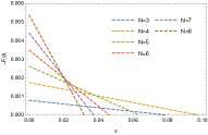
Figure 2: Bubble velocity excluding (left) and including (right) the reflection contribution.

References

- (1) J. S. Langer, Annals Phys. 54, 258-275 (1969).
- (2) L. P. Csernai and J. I. Kapusta, Phys. Rev. D 46, 1379-1390 (1992).
- (3) S. R. Coleman, Phys. Rev. D 15, 2929-2936 (1977) [erratum: Phys. Rev. D 16, 1248 (1977)] doi:10.1103/PhysRevD.16.1248
- (4) C. G. Callan, Jr. and S. R. Coleman, Phys. Rev. D 16, 1762-1768 (1977).
- (5) I. Affleck, Phys. Rev. Lett. 46, 388 (1981).
- (6) A. D. Linde, Nucl. Phys. B 216, 421 (1983) [erratum: Nucl. Phys. B 223, 544 (1983)].
- (7) A. M. Polyakov, Phys. Lett. B 72, 477-480 (1978).
- (8) L. Susskind, Phys. Rev. D 20, 2610-2618 (1979).
- (9) K. A. Olive, Nucl. Phys. B 190, 483-503 (1981).
- (10) E. Witten, Phys. Rev. D 30, 272-285 (1984) doi:10.1103/PhysRevD.30.272
- (11) L. D. McLerran and B. Svetitsky, Phys. Rev. D 24, 450 (1981).
- (12) V. Goloviznin and H. Satz, Z. Phys. C 57, 671-676 (1993).
- (13) A. Peshier, B. Kampfer, O. P. Pavlenko and G. Soff, Phys. Rev. D 54, 2399-2402 (1996).
- (14) R. D. Pisarski, Phys. Rev. D 62, 111501(R) (2000).
- (15) P. N. Meisinger, M. C. Ogilvie and T. R. Miller, Phys. Lett. B 585, 149-154 (2004).
- (16) M. Ruggieri, P. Alba, P. Castorina, S. Plumari, C. Ratti and V. Greco, Phys. Rev. D 86, 054007 (2012).
- (17) C. Sasaki and K. Redlich, Phys. Rev. D 86, 014007 (2012).
- (18) P. Alba, W. Alberico, M. Bluhm, V. Greco, C. Ratti and M. Ruggieri, Nucl. Phys. A 934, 41-51 (2014)
- (19) C. A. Islam, M. G. Mustafa, R. Ray and P. Singha, [arXiv:2109.13321 [hep-ph]].
- (20) J. Zhu, Z. Kang and J. Guo, Phys. Rev. D 107, no.7, 076005 (2023) doi:10.1103/PhysRevD.107.076005 [arXiv:2211.09442 [hep-ph]].
- (21) U. Reinosa, J. Serreau, M. Tissier and N. Wschebor, Phys. Lett. B 742, 61-68 (2015).
- (22) A. Dumitru, Y. Guo, Y. Hidaka, C. P. K. Altes and R. D. Pisarski, Phys. Rev. D 83, 034022 (2011).
- (23) A. Roberge and N. Weiss, Nucl. Phys. B 275, 734-745 (1986) doi:10.1016/0550-3213(86)90582-1
- (24) C. Sasaki and K. Redlich, Phys. Rev. C 79, 055207(R) (2009).
- (25) Y. Hidaka and R. D. Pisarski, Phys. Rev. D 78, 071501 (2008).
- (26) W. Cassing, Nucl. Phys. A 791, 365-381 (2007); W. Cassing, Nucl. Phys. A 795, 70-97 (2007).
- (27) G. D. Moore, JHEP 03, 006 (2000) doi:10.1088/1126-6708/2000/03/006 [arXiv:hep-ph/0001274 [hep-ph]].
- (28) T. Konstandin, G. Nardini and I. Rues, JCAP 09, 028 (2014) doi:10.1088/1475-7516/2014/09/028 [arXiv:1407.3132 [hep-ph]].
- (29) M. B. Hindmarsh, M. Lüben, J. Lumma and M. Pauly, SciPost Phys. Lect. Notes 24, 1 (2021) doi:10.21468/SciPostPhysLectNotes.24 [arXiv:2008.09136 [astro-ph.CO]].
- (30) M. Barroso Mancha, T. Prokopec and B. Swiezewska, JHEP 01, 070 (2021).
- (31) S. De Curtis, L. D. Rose, A. Guiggiani, Á. G. Muyor and G. Panico, JHEP 03, 163 (2022) doi:10.1007/JHEP03(2022)163 [arXiv:2201.08220 [hep-ph]].
- (32) B. Laurent and J. M. Cline, Phys. Rev. D 106, no.2, 023501 (2022) doi:10.1103/PhysRevD.106.023501 [arXiv:2204.13120 [hep-ph]].
- (33) S. De Curtis, L. Delle Rose, A. Guiggiani, Á. Gil Muyor and G. Panico, EPJ Web Conf. 270, 00035 (2022) doi:10.1051/epjconf/202227000035 [arXiv:2209.06509 [hep-ph]].
- (34) P. J. Steinhardt, Phys. Rev. D 25, 2074 (1982).
- (35) J. R. Espinosa, T. Konstandin, J. M. No and G. Servant, JCAP 06, 028 (2010).
- (36) W. Y. Ai, B. Garbrecht and C. Tamarit, JCAP 03, no.03, 015 (2022) doi:10.1088/1475-7516/2022/03/015 [arXiv:2109.13710 [hep-ph]].
- (37) L. Li, S. J. Wang and Z. Y. Yuwen, [arXiv:2302.10042 [hep-th]].
- (38) J. C. Wang, Z. Y. Yuwen, Y. S. Hao and S. J. Wang, [arXiv:2311.07347 [hep-ph]].
- (39) W. Y. Ai, X. Nagels and M. Vanvlasselaer, [arXiv:2401.05911 [hep-ph]].
- (40) K. Kajantie and H. Kurki-Suonio, Phys. Rev. D 34, 1719-1738 (1986).
- (41) J. Ignatius, K. Kajantie, H. Kurki-Suonio and M. Laine, Phys. Rev. D 49, 3854-3868 (1994) doi:10.1103/PhysRevD.49.3854 [arXiv:astro-ph/9309059 [astro-ph]].
- (42) Y. Bea, J. Casalderrey-Solana, T. Giannakopoulos, D. Mateos, M. Sanchez-Garitaonandia and M. Zilhão, Phys. Rev. D 104, no.12, L121903 (2021).
- (43) F. Bigazzi, A. Caddeo, T. Canneti and A. L. Cotrone, JHEP 08, 090 (2021) doi:10.1007/JHEP08(2021)090 [arXiv:2104.12817 [hep-ph]].
- (44) R. A. Janik, M. Jarvinen, H. Soltanpanahi and J. Sonnenschein, Phys. Rev. Lett. 129, no.8, 081601 (2022).
- (45) P. B. Arnold, Phys. Rev. D 48, 1539-1545 (1993) doi:10.1103/PhysRevD.48.1539 [arXiv:hep-ph/9302258 [hep-ph]].
- (46) D. Bodeker and G. D. Moore, JCAP 05, 009 (2009) doi:10.1088/1475-7516/2009/05/009 [arXiv:0903.4099 [hep-ph]].
- (47) D. Bodeker and G. D. Moore, JCAP 05, 025 (2017) doi:10.1088/1475-7516/2017/05/025 [arXiv:1703.08215 [hep-ph]].
- (48) A. Azatov and M. Vanvlasselaer, JCAP 01, 058 (2021) doi:10.1088/1475-7516/2021/01/058 [arXiv:2010.02590 [hep-ph]].
- (49) Y. Gouttenoire, R. Jinno and F. Sala, JHEP 05, 004 (2022) doi:10.1007/JHEP05(2022)004 [arXiv:2112.07686 [hep-ph]].
- (50) I. Baldes, Y. Gouttenoire and F. Sala, JHEP 04, 278 (2021) doi:10.1007/JHEP04(2021)278 [arXiv:2007.08440 [hep-ph]].
- (51) P. Schwaller, Phys. Rev. Lett. 115, no.18, 181101 (2015).
- (52) A. J. Helmboldt, J. Kubo and S. van der Woude, Phys. Rev. D 100, no.5, 055025 (2019) doi:10.1103/PhysRevD.100.055025 [arXiv:1904.07891 [hep-ph]].
- (53) J. Halverson, C. Long, A. Maiti, B. Nelson and G. Salinas, JHEP 05, 154 (2021) doi:10.1007/JHEP05(2021)154 [arXiv:2012.04071 [hep-ph]].
- (54) W. C. Huang, M. Reichert, F. Sannino and Z. W. Wang, Phys. Rev. D 104, no.3, 035005 (2021) doi:10.1103/PhysRevD.104.035005 [arXiv:2012.11614 [hep-ph]].
- (55) Z. Kang, J. Zhu and S. Matsuzaki, JHEP 09, 060 (2021).
- (56) M. Reichert, F. Sannino, Z. W. Wang and C. Zhang, JHEP 01, 003 (2022) doi:10.1007/JHEP01(2022)003 [arXiv:2109.11552 [hep-ph]].
- (57) E. Morgante, N. Ramberg and P. Schwaller, Phys. Rev. D 107, no.3, 036010 (2023).
- (58) Z. W. Wang, PoS ICHEP2022, 415 doi:10.22323/1.414.0415
- (59) K. Fujikura, Y. Nakai, R. Sato and Y. Wang, JHEP 09, 053 (2023) doi:10.1007/JHEP09(2023)053 [arXiv:2306.01305 [hep-ph]].
- (60) K. Fujikura, S. Girmohanta, Y. Nakai and M. Suzuki, Phys. Lett. B 846, 138203 (2023) doi:10.1016/j.physletb.2023.138203 [arXiv:2306.17086 [hep-ph]].
- (61) R. Pasechnik, M. Reichert, F. Sannino and Z. W. Wang, [arXiv:2309.16755 [hep-ph]].
- (62) Z. Kang and J. Zhu, work in progress.