Limitations of Data-Driven Spectral Reconstruction – An Optics-Aware Analysis

Abstract

Hyperspectral imaging empowers computer vision systems with the distinct capability of identifying materials through recording their spectral signatures. Recent efforts in data-driven spectral reconstruction aim at extracting spectral information from RGB images captured by cost-effective RGB cameras, instead of dedicated hardware.

In this paper we systematically analyze the performance of such methods, evaluating both the practical limitations with respect to current datasets and overfitting, as well as fundamental limits with respect to the nature of the information encoded in the RGB images, and the dependency of this information on the optical system of the camera.

We find that the current models are not robust under slight variations, e.g., in noise level or compression of the RGB file. Both the methods and the datasets are also limited in their ability to cope with metameric colors. This issue can in part be overcome with metameric data augmentation. Moreover, optical lens aberrations can help to improve the encoding of the metameric information into the RGB image, which paves the road towards higher performing spectral imaging and reconstruction approaches.

1 Introduction

(Hyper)spectral imaging is a method that involves recording the light in a scene in the form of many, relatively narrow, spectral bands, rather than projected into three broadband RGB color channels. Where RGB imaging utilizes the trichromaticity theory of human color vision, spectral imaging provides additional information that can help discriminate between different materials and lighting conditions that are hard to tell apart in RGB images. For example, red stains in a crime scene could be blood, or paint, or a dyed cloth, which cannot be distinguished from their RGB colors. Skin tumors could not be diagnosed from surrounding tissues of the same color. It is difficult to spot and sort out plastic leaves from living plants by their greenish colors. Therefore, spectral imaging has been applied in many fields, including machine vision [24, 47], healthcare [42], agriculture [21], and environment [9], to name just a few.

However, conventional hyperspectral cameras require scanning mechanisms [41, 31] to acquire the 3D hyperspectral datacube with 2D sensors. To simplify the demanding hardware, extensive efforts have been made in the development of various snapshot hyperspectral cameras [58, 49, 34]. In the computer vision community, deep learning methods have emerged to solve this challenging hardware problem with software reconstruction and data, resulting in three NTIRE challenges [5, 6, 7] and various network architectures [50, 38, 67, 13, 66].

Yet it remains unclear how these methods generalize to unseen data, how they deal with the difficult but important problem of resolving metamerism [28, 44], and how they depend on the optical system of both the RGB source and the spectral camera used to capture the training data.

In this paper, we take a systematic and outside-the-box look at all the aspects. By conducting a series of adversarial attacks and thorough analysis, we reveal a number of shortcomings in both current datasets and reconstruction methods. Specifically, we find that:

• Existing hyperspectral image datasets severely lack in diversity especially with respect to metameric colors but also other factors including nuisance parameters such as noise and compression ratios.

• State-of-the-art methods suffer from atypical overfitting problems that arise from various factors in the image simulation pipeline, such as noise, RGB data format, and lack of optical aberrations.

• Optical aberrations in RGB images, while currently ignored by all methods, are actually beneficial rather than harmful to spectral reconstruction.

• The utilization of metameric augmentation is crucial in the training and evaluation of neural networks for spectral reconstruction.

Through the evidence in this work, we contribute to a deepened understanding of the limitations of current datasets as well as of fundamental limitations in spectral reconstruction. The results on the interplay between metameric spectra and optical aberrations opens the door for new approaches for spectral recovery down the road.

2 Related Work

Hyperspectral cameras.

Conventional hyperspectral imaging systems require filter wheels, liquid-crystal tunable filters, or mechanical motion (e.g., pushbroom) [41, 31] to scan the 3D hyperspectral datacube. To enable snapshot acquisition, coded-aperture snapshot spectral imager (CASSI) [58, 18] has been proposed to achieve high spectral accuracy using spectrum-dependent coded patterns. Recent methods also exploit spectrally encoded point spread functions (PSFs) to computationally reconstruct a hyperspectral image [34, 8, 14]. In general, great efforts have been made to simplify hyperspectral camera hardware by software reconstruction.

Spectral reconstruction from RGB images.

A recent trend to solve the snapshot hyperspectral imaging problem is to exploit hyperspectral data with deep neural networks to reconstruct spectral information from RGB images [4]. Owing to the wide availability of RGB cameras, this approach seems to be a promising candidate for hyperspectral imaging if successful. A large number of neural network architectures have been proposed in the past three NTIRE spectral recovery challenges  [5, 6, 7]. Our analysis in this paper focuses on this class of methods to gain insights on their strengths and limitations.

Dataset bias and data augmentation.

Deep neural networks are prone to suffer from data bias [53, 23] and overfitting problems [10]. Overfitting can lead to the inability of trained models to generalize in real-world applications [36]. Although overfitting can sometimes be detected by inspecting the training and validation performance over the course of training, it can often be imperceivable in challenging problems. A useful technique to detect overfitting is to use adversarial examples [60] generated from the original dataset. On the other hand, it is important to address overfitting when the amount of data is limited. Data augmentation [51, 48] techniques are usually employed to improve the robustness of deep neural networks.

Metamerism.

Metamerism is a physical phenomenon where distinct spectra produce the same color [2] as the high-dimensional spectral space is projected down to three dimensions of a trichromatic vision system (either the human eye or an RGB camera). This phenomenon has been studied in color science [52, 27], spectral rendering [33, 59, 54], and hyperspectral imaging [28, 26]. In hyperspectral imaging [20, 44], it is crucial for many applications to distinguish between metamers or near-metamers (i.e., different spectra that project to similar RGB values). Indeed spectral imaging is usually employed when the RGB color differences between two materials or features are too small to reliably distinguish between them. Therefore, hyperspectral imaging systems require special attention in the system design to acquire accurate spectral signatures [29, 35].

3 Fundamentals

Spectral image formation.

We denote the hyperspectral image as a matrix ${\mathbf{X}}\in\mathbb{R}^{MN\times K}$, where $M,N$ are the number of pixels, and $K$ is the number of spectral bands. Note that we have stacked the 2D spatial dimensions in rows of ${\mathbf{X}}$. The spectral response function (SRF) of the camera can be expressed as a matrix ${\mathbf{Q}}\in\mathbb{R}^{K\times 3}$. Therefore, the spectrum-to-color projection results in a color image

$${\mathbf{Y}}={\mathbf{X}}{\mathbf{Q}},$$ (1)

where ${\mathbf{Y}}\in\mathbb{R}^{MN\times 3}$. This is the color formation model in the NTIRE 2022 challenge [7]. The inverse problem is to recover ${\mathbf{X}}$ from ${\mathbf{Y}}$.

In the past NTIRE challenges [5, 6, 7], optical aberrations haven’t been included in the image simulation pipeline. However, the optical system of the RGB camera inevitably introduces spectrally-varying blurs to the spectral images, which is modeled as PSFs. This optical process can be described by a linear matrix-vector product in each spectral band followed by a sum over the spectral dimension. The spectral images through the optical system are ${\mathbf{W}}=\mathrm{diag}\left({\mathbf{A}}{\mathbf{X}}\right)$, where ${\mathbf{A}}\in\mathbb{R}^{KMN\times MN}$ is a block matrix that stacks the spectral PSF matrices vertically, and $\mathrm{diag}(\cdot)$ extracts the diagonal blocks. The final RGB image is then

$${\mathbf{Z}}=\mathrm{diag}\left({\mathbf{A}}{\mathbf{X}}\right){\mathbf{Q}},$$ (2)

where ${\mathbf{Z}}\in\mathbb{R}^{MN\times 3}$. With the optical image formation model accounted for, the inverse problem is to recover ${\mathbf{X}}$ from ${\mathbf{Z}}$. See Supplement for details.

Hyperspectral datasets and data diversity.

Compared to very large color (RGB) image datasets (e.g., ImageNet [22], DIV2K [1]), hyperspectral datasets are far smaller in size, primarily limited by the unavailability of high-quality hyperspectral cameras and the difficulty in acquiring outside the lab with moving target scenes. The largest dataset so far is ARAD1K used in the NTIRE 2022 challenge [7]. In addition, we also include the CAVE [62], ICVL [4], and KAUST [39] datasets that share the same spectral range to extend our experiments. The datasets are summarized in Table 1. Although other datasets [15, 17, 43] exist, they cover slightly different spectral bands, making direct comparisons difficult. We therefore restrict our analysis to the datasets listed in the table.

Dataset	Spectra (nm)	Resolution (x, y, $\lambda$)	Amount	Device	Scene
CAVE [62]	400:10:700	512 $\times$ 512 $\times$ 31	32	monochrome sensor + tunable filters	lab setup
ICVL [4]	400:10:700	1392 $\times$ 1300 $\times$ 31	201	HS camera (Specim PS Kappa DX4)	outdoor
KAUST [39]	400:10:700	512 $\times$ 512 $\times$ 31	409	HS camera (Specim IQ)	outdoor
ARAD1K [7]	400:10:700	482 $\times$ 512 $\times$ 31	1000	HS camera (Specim IQ)	outdoor

Table 1: Basic information of four existing hyperspectral datasets.

The difficulties in the data capture not only affect the size but also the diversity of the datasets. In particular, effects like metamerism, which are comparatively rare in everyday environments [27, 46], yet crucial for many actual applications of spectral imaging, are under-represented in the datasets. While the CAVE dataset [62] contains some fake-and-real pairs of objects to account for metamerism, the total amount of such data is still very low. We analyze the general data diversity issue in Section 4 and the specific case of metamerism in Section 5.

Spectral augmentation with metamers.

Since it is difficult to provide enough examples of metamerism in small datasets, we propose a new form of data augmentation in our experiments. Metameric augmentation starts with existing spectral images and creates a new, different spectral image that however maps to the same RGB image (given a specific set of RGB spectral response functions).

Interestingly, metamer generation from existing spectra has been studied in color science and spectral rendering to accurately model the scenes using various methods, e.g., metameric black [56, 25, 3] and spectral upsampling [33, 54, 11]. In this work, we adopt the metameric black approach to generate metamers. A spectrum ${\mathbf{S}}$ can be projected onto two orthogonal subspaces, one for the fundamental metamer ${\mathbf{S}}^{*}$, and the other for metameric black ${\mathbf{B}}$ [19, 57]. A new metameric spectrum ${\mathbf{S}}^{\prime}$ is then

$${\mathbf{S}}^{\prime}={\mathbf{S}}^{*}+\alpha{\mathbf{B}},$$ (3)

where ${\mathbf{S}}^{*}={\mathbf{Q}}\left({\mathbf{Q}}^{T}{\mathbf{Q}}\right)^{-1}{\mathbf{Q}}^{T}{\mathbf{S}}$ and ${\mathbf{B}}={\mathbf{S}}-{\mathbf{S}}^{*}$. Since adding metameric black does not alter the RGB color, we can vary the coefficient $\alpha$ to generate different spectra that are all metamers. To avoid negative spectral radiance, we clip the negative values in the generated spectra and re-calculate the RGB colors for the affected pixels.

Performance evaluation metrics.

Consider a hyperspectral image ${\mathbf{X}}_{k,i,j}$ and its estimate $\hat{{\mathbf{X}}}_{k,i,j}$, where $k$ is the spectral index, and $i,j$ are spatial indices. The reconstruction quality can be evaluated in various ways. The NTIRE 2022 spectral reconstruction challenge [7] adopts two numerical metrics, Mean Relative Absolute Error (MRAE), and Root Mean Square Error (RMSE):

$${\mathrm{\mathbf{MRAE}}}=\frac{1}{KMN}\sum_{k,i,j}\left|\hat{{\mathbf{X}}}_{k,i,j}-{\mathbf{X}}_{k,i,j}\right|/{\mathbf{X}}_{k,i,j},$$ (4)

$${\mathrm{\mathbf{RMSE}}}=\sqrt{\frac{1}{KMN}\sum_{k,i,j}\left(\hat{{\mathbf{X}}}_{k,i,j}-{\mathbf{X}}_{k,i,j}\right)^{2}}.$$ (5)

Another metric widely used in hyperspectral imaging is the Spectral Angle Mapper (SAM) [55, 37, 45], although it has not yet found its way into the relevant computer vision literature. SAM emphasizes the spectral accuracy compared to the previous metrics, which are more forgiving of large errors in individual spectral channels:

$${\mathrm{\mathbf{SAM}}}=\frac{1}{MN}\sum_{i,j}\cos^{-1}\left(\frac{\sum_{k}\hat{{\mathbf{X}}}_{k,i,j}{\mathbf{X}}_{k,i,j}}{\sqrt{\sum_{k}\hat{{\mathbf{X}}}_{k,i,j}^{2}\sum_{k}{\mathbf{X}}_{k,i,j}^{2}}}\right).$$ (6)

Finally, we also inspect the spatial quality in individual spectral channels, and calculate the spectrally averaged Peak Signal-to-Noise Ratio (PSNR),

$${\mathrm{\mathbf{PSNR}}}=\frac{1}{K}\sum_{k}20\log_{10}\left(\frac{\textrm{MAX}}{\sqrt{\textrm{MSE}_{k}}}\right),$$ (7)

where MAX is the maximum possible value, and $\textrm{MSE}_{k}$ is the mean squared error in the $k$-th spectral band. This metric complements RMSE to account for performance variation in individual spectral bands.

Training details.

In our study, we use a single A100 GPU (80 GB memory) to conduct experiments across various datasets and network architectures. Adhering to the methodologies proposed by the latest champion network MST++ [13], we employ their overlapping patch-wise training approach (patches of 128$\times$128 pixels). The validation is on the full resolution. See Supplement for details.

4 Finding 1: Atypical Overfitting

Although it is well-known that deep neural networks may suffer from overfitting problems, we find that the overfitting behavior in spectral reconstruction is atypical and difficult to notice with standard evaluations. Here we introduce minimalist changes to the ARAD1K dataset used in NTIRE 2022 challenge [7] in three experiments to demonstrate it.

Training with less data.

First, we make a simple change to the training of the participating networks in the NTIRE 2022 challenge [7]. While keeping all the training settings intact, we randomly choose only 50% or 20% of the original training data respectively to train the candidate networks, and validate the performance on the original validation data. We illustrate the validation curves for MST++ [13] in Fig. 1. See Supplement for the results of other networks. We summarize the results for 100% and 50% training data in Table 2 for all networks.

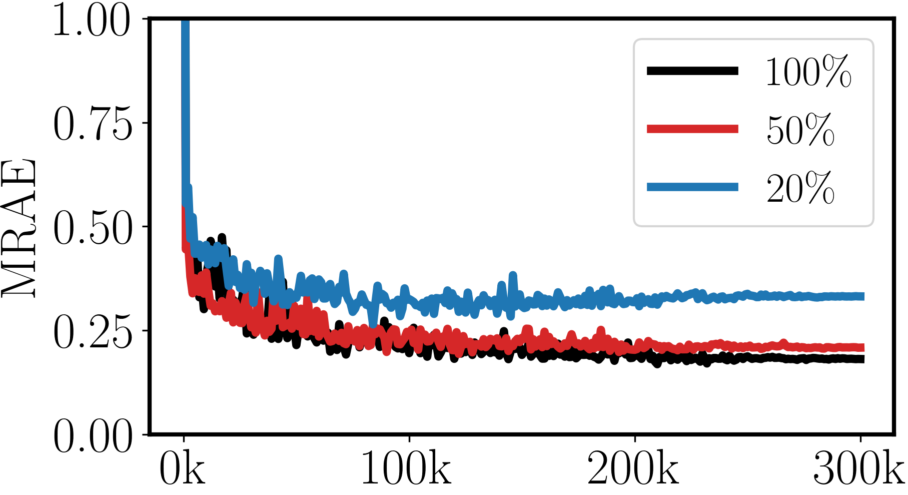
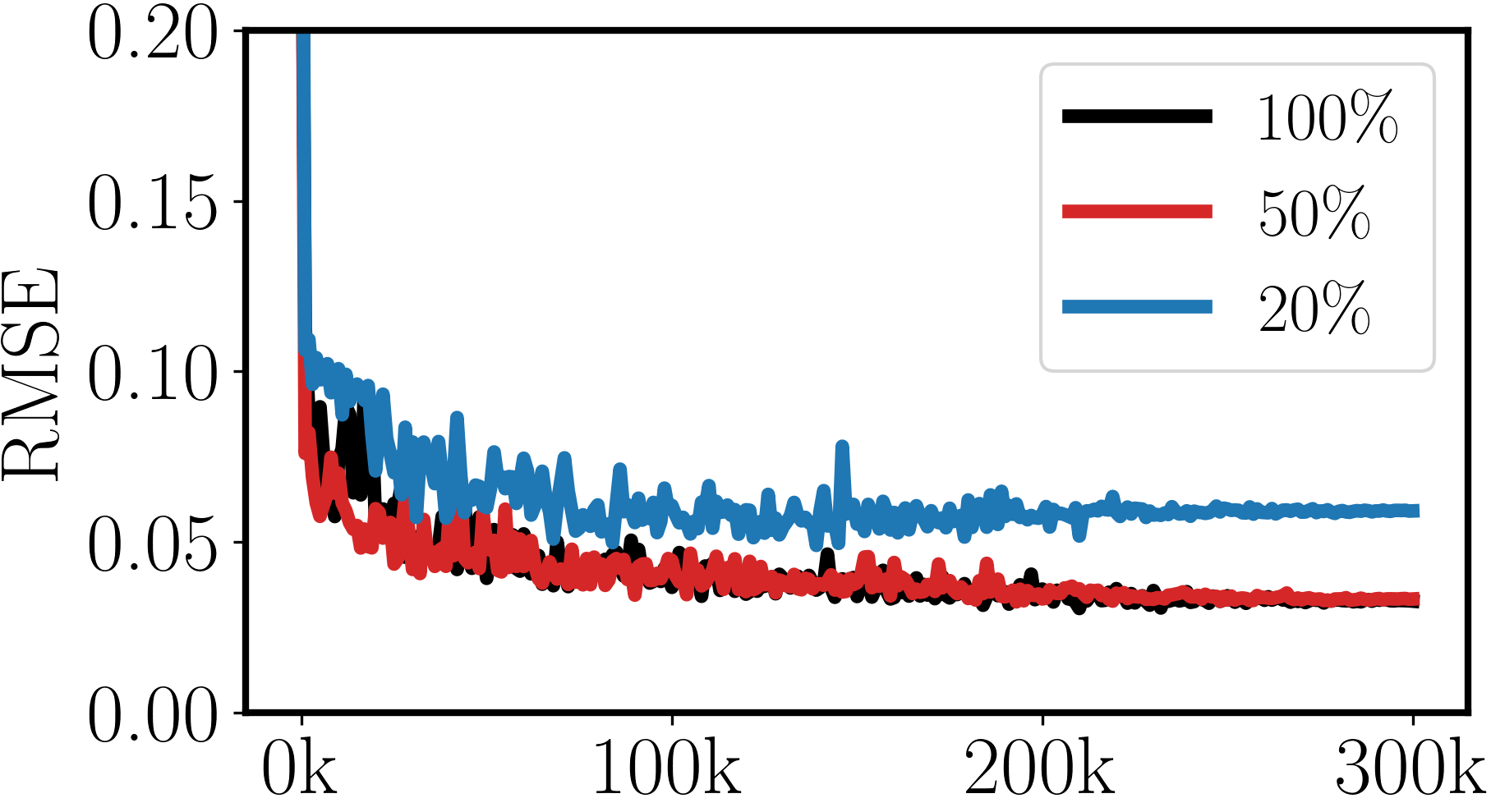
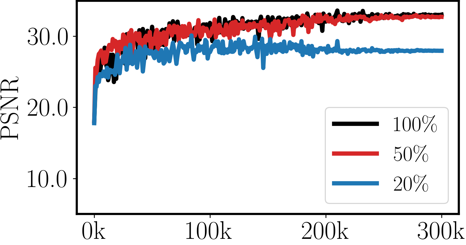
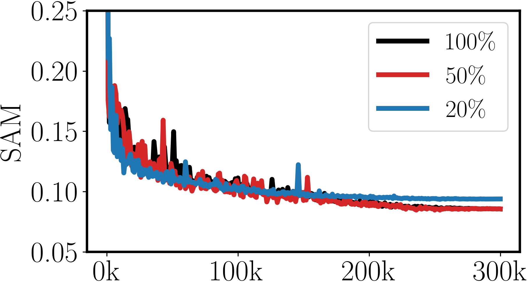
Figure 1: Validation performance for MST++ [13] with 100%, 50%, and 20% of the original training data on ARAD1K [7].

Although the performance with less training data deviates mildly in MRAE, RMSE, and PSNR, the spectral accuracy SAM (highlighted in bold in Table 2) is surprisingly less affected. In particular, some networks (e.g., MST++ [13], MIRNet [63]) achieve exactly the same SAM scores. MST-L [12] (50%) even improves SAM slightly, placing itself the best among all.

Network	Data	MRAE$\downarrow$	RMSE$\downarrow$	PSNR$\uparrow$	SAM$\downarrow$
MST++[13]	100%	0.182	0.033	33.0	0.086
	50%	0.209	0.033	32.7	0.086
MST-L[12]	100%	0.184	0.031	33.5	0.084
	50%	0.253	0.042	30.6	0.080
MPRNet[64]	100%	0.212	0.034	32.5	0.084
	50%	0.293	0.039	31.3	0.091
Restormer[65]	100%	0.204	0.033	33.2	0.083
	50%	0.304	0.041	31.4	0.092
MIRNet[63]	100%	0.186	0.030	33.7	0.082
	50%	0.214	0.033	32.6	0.082
HINet[16]	100%	0.234	0.036	32.3	0.085
	50%	0.267	0.041	30.7	0.090
HDNet[30]	100%	0.223	0.038	31.2	0.095
	50%	0.296	0.047	28.9	0.097
AWAN[38]	100%	0.213	0.034	32.2	0.091
	50%	0.273	0.042	30.5	0.095
EDSR[40]	100%	0.358	0.052	27.3	0.095
	50%	0.430	0.059	26.1	0.093
HRNet[67]	100%	0.388	0.057	26.4	0.094
	50%	0.413	0.065	25.5	0.096
HSCNN+[50]	100%	0.428	0.066	25.4	0.098
	50%	0.462	0.068	25.0	0.101

Table 2: Performance comparison with 100% and 50% of training data for different methods on the original ARAD1K dataset.

We therefore paradoxically find that despite the small size of hyperspectral datasets, the data already seems to be redundant. This serves as a first indication that the diversity of the datasets is severely lacking. We analyze this effect in more depth in the following experiments.

Validation with unseen data.

To further scrutinize the underlying issue, we validate existing pre-trained models with “unseen” data synthesized from the original dataset used in the NTIRE challenge. The challenge organizers state that

the exact noise parameters and JPEG compression level used to generate RGB images for the challenge was kept confidential

[7]. Only the spectrum-to-color projection was considered, and no aberrations of the optical system were simulated.

In our experiments, we generate new RGB images using the same methodology and calibration data, but different noise and compression settings. Specifically, we use the SRF data for a Basler ace 2 camera (model A2a5320-23ucBAS) known to the networks, and simulate Poisson noise at varying noise levels by controlling the number of photon electrons (npe). We adopt the same rudimentary in-camera image signal processing pipeline. As an illustrative example, we use MST++ [13] in Table LABEL:tab:unseen, Row 1 as a reference for comparison; results for other networks can be found in the Supplement.

	Data property				MRAE $\downarrow$	RMSE $\downarrow$	PSNR $\uparrow$	SAM $\downarrow$
	Data source	Noise (npe)	RGB format	Aberration
1	NTIRE 2022	unknown	jpg (Q unknown)	None	0.170	0.029	33.8	0.084
2	Synthesized	0	jpg (Q = 65)	None	0.460	0.049	29.2	0.094
3		0	png (lossless)	None	0.362	0.057	28.7	0.087
4		1000	png (lossless)	CA*	0.312	0.055	28.4	0.118

First, as a baseline, we consider a noiseless (npe = 0) and aberration-free case with moderate JPEG compression quality (Q = 65), shown in Table LABEL:tab:unseen, Row 2. The results show significant drops in all the performance metrics. Note that the only differences here compared to the challenge dataset are the noise level and compression quality – the base images are identical! This indicates that the network overfits both the noise and JPEG compression parameters.

Second, in Row 3, we generate noiseless RGB images, but in lossless PNG format. Note that JPEG compression is not necessary for the core inverse problem in hyperspectral imaging, since raw data could be readily obtained from the sensors. This results in paradoxical reconstruction performance. MRAE and SAM improve compared to Row 2 (but are still worse than Row 1), while RMSE and PSNR deteriorate further. Considering this only eliminates image compression, and the networks were trained on MRAE [13], we can confirm that the network indeed overfits the specific unknown JPEG compression used in the challenge [7].

Third, we consider a more realistic imaging scenario, in which we eliminate the impact of unnecessary compression by employing the lossless PNG format to save the RGB images (equivalent to using raw camera data). We adopt moderate noise levels (npe = 1000) and realistic optical aberrations from a recent double Gauss lens patent [32] to mimic a real photographic camera. We can observe a further performance drop in Row 4, which provides additional evidence that the network overfits the unknown parameters in the image simulation pipeline [7]. When used under realistic imaging conditions, the performance degrades significantly.

Cross-dataset validation.

In addition, we also inspect the effects of different datasets (cf. Table 1) on the performance. We train the MST++ network on the four datasets with the same image simulation parameters. To eliminate the impact of other factors, we choose the ideal noiseless and aberration-free condition without compression. In the validation, we use our trained model on ARAD1K dataset to validate on the other three datasets, respectively. In Table 4, we compare the performance with the models both trained and validated on the original datasets. Results for other networks can be found in the Supplement. They all illustrate the same difficulties in generalization.

Trained on	Validated on	MRAE$\downarrow$	RMSE$\downarrow$	PSNR$\uparrow$	SAM$\downarrow$
CAVE	CAVE	0.237	0.034	31.9	0.194
ARAD1K	CAVE	1.626	0.074	24.4	0.376
ICVL	ICVL	0.079	0.019	38.3	0.024
ARAD1K	ICVL	0.627	0.091	22.0	0.110
KAUST	KAUST	0.069	0.013	44.4	0.061
ARAD1K	KAUST	1.042	0.100	22.0	0.370

Table 4: Cross-dataset validation example using MST++ [13].

Even though the imaging conditions are the same and ideal, the network trained on one dataset experiences significant performance drop in all metrics when validated on other datasets. This indicates that the contents of the datasets, as well as the acquisition devices used to capture the datasets, play important roles.

We also point out that the CAVE dataset [62], although smaller and older than the others, is more difficult to train for better performance. This is probably due to the fact that CAVE consists of several challenging scenes of real and fake objects that appear in similar colors, but other datasets comprise less aggressive natural scenes.

Discussion.

The experiments conducted in this section clearly highlight several shortcomings with respect to the existing datasets: (1) they lack diversity in nuisance parameters such as noise and compression ratios, and (2) they lack scene diversity. While we show in this document the results for the largest available dataset (ARAD1K), the Supplement shows consistent results for all the datasets. Both of these aspects result in over-fitting and prevent the networks from learning the general spectral image restoration task. Next we specifically analyze the effect of metamerism; the analysis of the impact of optical aberrations will be deepened in Section 6.

5 Finding 2: Metameric Failure

In this section, we first inspect the performance of existing methods using metamer as an adversary, and then employ it for spectral augmentation to re-train the neural networks for further analysis.

Validation with metamers.

We generate metamer datacubes (metamer data) from the original ARAD1K dataset (standard data) using the metameric black method [25]. For this set of experiments, we fix the coefficient $\alpha=0$ in Eq. (3). We choose a realistic imaging condition as used in Table LABEL:tab:unseen, Row 4, and keep it the same for both cases. The validation results on the ARAD1K dataset for existing pre-trained networks are summarized in Table 5. We also visualize the reconstructed spectral images in five arbitrary bands (420 nm, 500 nm, 550 nm, 580 nm, and 660 nm) and spectra of two points in Fig. 2 for Scene ARAD_1K_0944 from the validation set.

Network	Data	MRAE$\downarrow$	RMSE$\downarrow$	PSNR$\uparrow$	SAM$\downarrow$
MST++[13]	std	0.312	0.055	33.8	0.084
	met	52.839	0.091	26.0	0.580
MST-L[12]	std	0.327	0.055	28.0	0.118
	met	51.321	0.090	25.9	0.579
MPRNet[64]	std	0.661	0.066	26.1	0.125
	met	145.981	0.122	23.3	0.547
Restormer[65]	std	0.510	0.066	25.5	0.126
	met	79.705	0.116	23.4	0.567
MIRNet[63]	std	0.404	0.077	24.8	0.124
	met	38.252	0.089	24.8	0.570
HINet[16]	std	0.450	0.063	26.5	0.120
	met	67.148	0.096	24.8	0.552
HDNet[30]	std	0.450	0.082	23.9	0.126
	met	34.429	0.095	23.8	0.570
AWAN[38]	std	0.424	0.080	24.6	0.119
	met	39.854	0.095	24.4	0.558
EDSR[40]	std	0.421	0.066	25.5	0.132
	met	49.435	0.100	23.8	0.564
HRNet[67]	std	0.514	0.078	23.9	0.128
	met	43.726	0.112	22.7	0.560
HSCNN+[50]	std	0.508	0.075	24.4	0.148
	met	42.274	0.098	23.1	0.556

Table 5: Validation performance for different pre-trained models on standard (std) data and metamer (met) adversary synthesized from the ARAD1K dataset [7].

Figure 2: Validation with metamers for MST++ [13]. An example Scene ARAD_1K_0944 is shown to visualize the standard and metamer datacubes. Top left: the standard and metamer data result in similar color images. Bottom left: ground-truth and reconstructed spectra from two labeled points. Right: ground-truth and reconstructed spectral images in 420 nm, 500 nm, 550 nm, 580 nm, and 660 nm.

From the numerical results in Table 5, it is apparent that all the existing methods experience catastrophic performance drop in terms of MRAE and SAM in the presence of metamers, which we call metameric failure. The MRAE (cf. Eq. (4)) may yield large values when big errors occur for dark ground-truth pixels (see the exemplary spectra in Fig. 2). The SAM values become large when the spectra are essentially dissimilar with each other. RMSE and PSNR do not capture the spectral differences as well, since they average out differences in the spatial and spectral dimensions.

The visual results in Fig. 2 show that the reconstruction results are very close to each other for both standard and metamer data, because the input RGB images are quite similar. However, distinct differences exist in the scene for certain spectral bands, e.g., the intensities of the yellow and green parts of the slide (blue box) in 500 nm band vary in the standard data, but remain identical in the metamer data. The reconstructions fail to reflect this important difference. All spectral images are displayed on the same global intensity scale, so the brightness differences (green box) in corresponding images reflect the reconstruction artifacts for the metamer data.

Training with metamers.

The pre-trained models were not explicitly trained to cope with metamers. This raises the question whether it is possible to improve the performance by training the networks with metamer data. As a first step, we use both the standard and metamer data ($\alpha=0$) generated from the ARAD1K dataset to train various networks. To eliminate the impact of other factors, we simulate the RGB images in a noiseless, aberration-free condition, and without compression.

As a second variant, we train the neural networks with random metamers generated on-the-fly as a spectral augmentation to enhance the spectral content of existing datasets. We vary the coefficient for the metameric black by setting $\alpha$ as a uniformly distributed random number in the range $[-1,2]$. During validation, we use both the standard validation data and their corresponding metamer data with fixed $\alpha=0$, which doubles the amount of the original validation data.

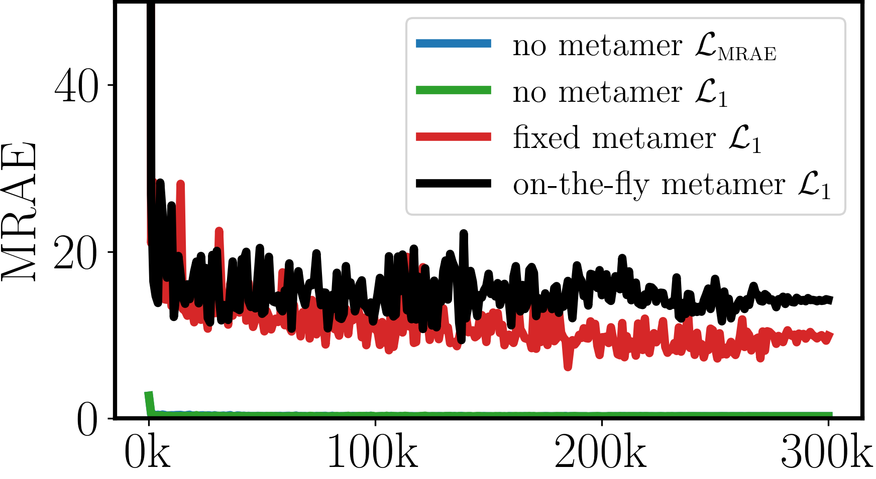
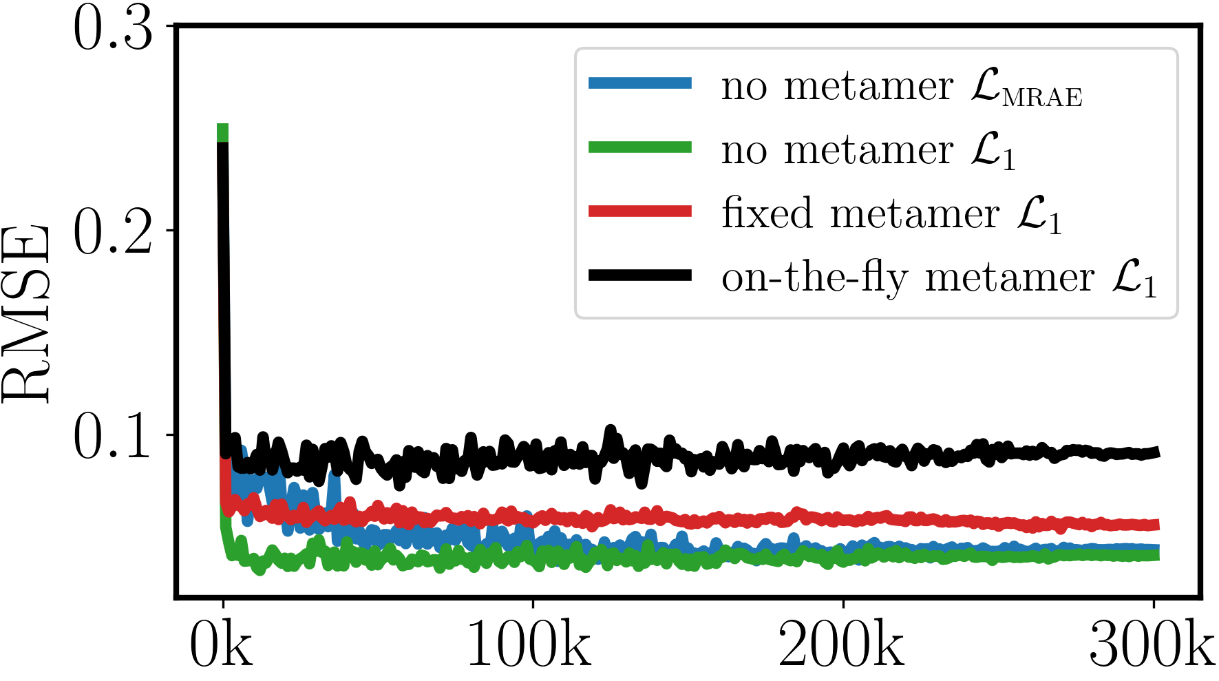
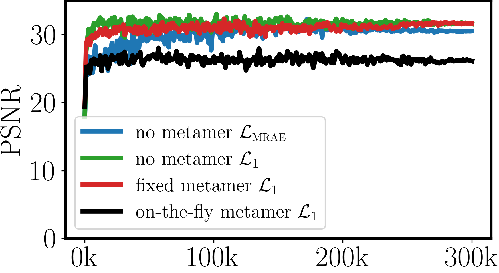
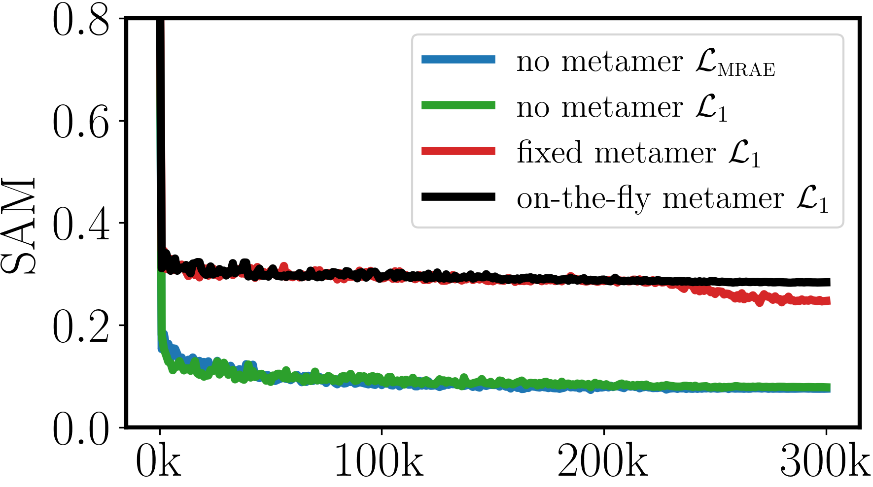
Figure 3: Training MST++ with metamers. The network fails to combat fixed metamers and on-the-fly metamers, in particular on the spectral accuracy SAM.

As an example, we train MST++ and evaluate its validation performance over the training process. In Fig. 3, we show that it is no longer a good choice to use MRAE as the loss function [13] and evaluation metric [7], because it is completely overwhelmed by metamers. Instead, we find that L1 loss is a more stable loss function, so we train the network with L1 loss for three cases, no metamer (easy), fixed metamer (medium), and on-the-fly metamer (difficult). Nevertheless, we can see in Fig. 3 that the network fails in particular for the spectral accuracy SAM.

Network	Metamer	MRAE$\downarrow$	RMSE$\downarrow$	PSNR$\uparrow$	SAM$\downarrow$
MST++[13]	no	0.270	0.041	31.6	0.079
	fixed	9.912	0.056	31.6	0.247
	on-the-fly	14.224	0.091	26.1	0.284
MST-L[12]	no	0.269	0.040	32.2	0.081
	fixed	11.398	0.061	30.2	0.289
	on-the-fly	12.155	0.061	27.0	0.258
MPRNet[64]	no	0.346	0.051	29.9	0.076
	fixed	7.359	0.059	30.6	0.224
	on-the-fly	13.492	0.087	26.6	0.264
Restormer[65]	no	0.286	0.041	31.5	0.068
	fixed	8.129	0.059	31.0	0.242
	on-the-fly	10.186	0.089	26.7	0.264
MIRNet[63]	no	0.258	0.040	32.2	0.083
	fixed	9.555	0.061	30.5	0.289
	on-the-fly	13.205	0.088	26.4	0.290
HINet[16]	no	0.315	0.056	28.0	0.081
	fixed	8.322	0.068	29.6	0.296
	on-the-fly	14.238	0.090	25.5	0.288
HDNet[30]	no	0.287	0.045	30.2	0.087
	fixed	8.884	0.064	30.2	0.296
	on-the-fly	18.270	0.087	26.4	0.299
AWAN[38]	no	0.240	0.039	32.0	0.073
	fixed	8.789	0.068	29.6	0.294
	on-the-fly	14.406	0.090	26.0	0.264
EDSR[40]	no	0.415	0.061	26.1	0.084
	fixed	9.717	0.073	26.6	0.297
	on-the-fly	11.723	0.101	23.2	0.290
HRNet[67]	no	0.430	0.065	25.6	0.085
	fixed	8.142	0.076	26.0	0.299
	on-the-fly	13.098	0.103	23.0	0.294
HSCNN+[50]	no	0.516	0.077	24.1	0.082
	fixed	9.362	0.085	24.8	0.297
	on-the-fly	13.311	0.102	22.9	0.286

Table 6: Performance comparison for training various networks with fixed and on-the-fly metamers.

We also train all other candidate networks with fixed and on-the-fly metamers. The results are summarized in Table 6. Again, the same performance drop applies to all networks. Finally, we show the results of the top-performing network, MST++ on the CAVE, ICVL, and KAUST datasets (Table 7, Supplement). As before, the performance drops similarly in the presence of metamers.

Dataset	Metamer	MRAE$\downarrow$	RMSE$\downarrow$	PSNR$\uparrow$	SAM$\downarrow$
CAVE[62]	no	1.014	0.038	29.9	0.192
	fixed	38.26	0.053	29.6	0.229
	on-the-fly	226.0	0.078	25.2	0.451
ICVL[4]	no	0.067	0.016	40.1	0.027
	fixed	1.454	0.041	34.8	0.229
	on-the-fly	2.615	0.087	24.3	0.268
KAUST[39]	no	0.082	0.016	43.2	0.076
	fixed	2.033	0.022	39.0	0.217
	on-the-fly	1.874	0.032	33.7	0.245

Table 7: Training with metamers for MST++ on the CAVE, ICVL, and KAUST datasets.

Discussion.

The experiments conducted in this section clearly highlight the difficulties that the data-driven spectral recovery methods face with metamers: (1) lack of sufficient metameric data in current datasets, (2) metameric augmentation can help overcome this issue, but (3) spectral estimation from RGB data is fundamentally limited in the presence of metamers.

The limitations of spectral estimation from RGB data are ultimately not overly surprising – after all the projection from the high dimensional spectral space to RGB invariably destroys scene information that can be difficult to recover. However, our experiments show that this is indeed an issue faced by the state-of-the art methods, which so far went unnoticed due to the under-representation of metamers in the datasets. This shortcoming will also affect other uses of the same datasets, for example in the training of reconstruction methods for spectral computational cameras [34, 8, 14]. Metameric augmentation can help to overcome this issue, although datasets with more genuine metamers would certainly be highly desirable.

6 Finding 3: The Aberration Advantage

As shown so far, the existing methods have difficulties distinguishing metamers in the ideal noiseless and aberration-free condition. In this section, we analyze what effect (if any) optical aberrations have on this situation, i.e., aberration-aware training [61]. To this end we train the networks in a realistic imaging condition with moderate noise level (npe = 1000), lossless PNG format, and aberrations from the same double Gauss lens as before [32]. In short, we simulate, through spectral ray tracing, the effect that an imperfect (i.e., aberrated) optical system has on the RGB image measured when observing a specific spectral scene. The details of this simulation can be found in the Supplement.

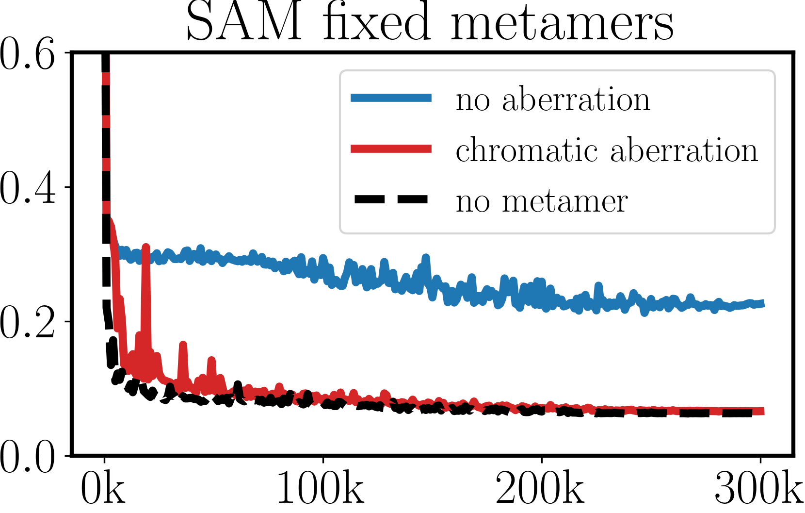
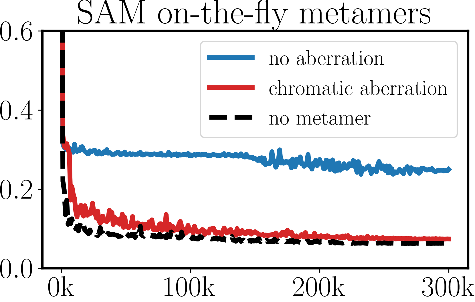
Figure 4: Chromatic aberrations improve spectral accuracy. Left: fixed metamers. Right: on-the-fly metamers.

In Fig. 4, we show an example with MST++ for the validation on SAM in two situations, one with fixed metamers, and the other with on-the-fly metamers. In each experiment, we compare the SAM difference with and without aberrations. As a reference, we also show the standard validation without metamers. As we can see, the realistic optical aberrations of the lens actually improve the spectral estimation in the presence of metamers as long as the aberrations are modeled in the training. With chromatic aberrations, the network can already distinguish fixed metamer pairs, achieving similar accuracy as the standard case. In the more aggressive case of on-the-fly metamers, chromatic aberrations also improve the spectral accuracy, compared with its no-aberration counterpart. Again, this aberration advantage holds for all datasets (Table 8). See Supplement for details.

Dataset	Fixed metamers		On-the-fly metamers
	no aberration	aberration	no aberration	aberration
CAVE[62]	0.251	0.135	0.380	0.167
ICVL[4]	0.028	0.077	0.240	0.085
KAUST[39]	0.212	0.113	0.221	0.113

Table 8: SAM metrics for MST++ on CAVE, ICVL, and KAUST.

Discussion.

To understand why optical aberrations help improve the reconstruction, consider the simulated images in Fig. 5. The left and middle image are simulations of RGB images for metameric scene pairs, with the difference image on the right. The different spectra of the two scenes are affected differently by the optical aberrations, and therefore, although the scenes are metamers of each other, the RGB images are in fact different. In effect, the optical aberrations have encoded spectral information into the RGB image, which the networks can learn to distinguish, lending credibility to PSF engineering methods for hyperspectral encoding [34, 8, 14].

standard	metamer	color difference

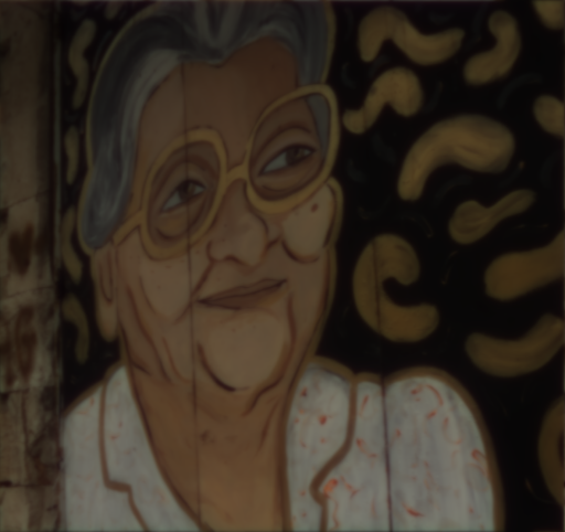
Figure 5: Chromatic aberration induced informative color differences (right) as spectral cues for metamer pairs (left and middle).

There are however, also detrimental consequences of this effect, namely (1) “baked-in” aberrations in spectral datasets and (2) limited generalization to arbitrary RGB image sources.

Regarding (1), it is worth noting that even expensive spectral cameras typically do not have diffraction limited optics, i.e., their optical systems are aberrated. In order to avoid overfitting to these aberrations, future datasets should ideally be collected with a large variety of different spectral cameras.

With respect to (2) we note that different RGB cameras produce very different aberrations, and often the aberrations also vary significantly across the image plane. Without further improvements on the reconstruction methods, this will result in large device dependency and poor generalization of the methods.

7 Conclusion

In this work, we have comprehensively analyzed a category of data-driven spectral reconstruction methods from RGB images by reviewing the problem fundamentally from dataset bias to physical image formation, and to reconstruction networks. From an optics-aware perspective, we leverage both metamerism and optical aberrations to reassess existing methodologies.

The major findings of our study are that (1) the limitations of current datasets lead to overfitting to both nuisance parameters (noise, compression), as well as limited scene content. (2) Metamerism in particular presents a challenge both in terms of under-representation in the datasets, and in terms of fundamental limits of spectral reconstruction from RGB input. (3) Metameric augmentation can help to alleviate the dataset issue, while (4) the targeted use of optical aberrations enables resolving the metamer issue.

In particular the last point lends additional credibility to computational camera approaches for spectral imaging, including both PSF engineering approaches [34, 8, 14] and compressed sensing methods like CASSI [58, 18]. However, learned reconstruction methods for these approaches will suffer from the same dataset issues as the methods analyzed in this paper, making the collection of large-scale, diverse spectral image data a matter of urgency.

In order to realize the dream of spectral estimation from arbitrary RGB sources it will be necessary to devise completely new data augmentation methods and network architectures that can adapt to whole families of aberrations or effectively use metadata to condition the reconstruction.

Supplementary Material

8 Image Formation Model

Mathematically, the physical image formation of a color image from the spectral radiance can be expressed by

$$g_{c}\left(x,y\right)=\int_{\lambda_{1}}^{\lambda_{2}}\left(f\left(x,y,\lambda\right)*h\left(x,y,\lambda\right)\right)q_{c}\left(\lambda\right)d\lambda,$$ (8)

where $f\left(x,y,\lambda\right)$ is the spectral image, $h\left(x,y,\lambda\right)$ is the spectral point spread function (PSF) of the optical system, $q_{c}\left(\lambda\right)$ is the spectral response function (SRF) of the sensor, and $g_{c}\left(x,y\right)$ is the color image in color channel $c\in[R,G,B]$.

Let us denote the hyperspectral image as a matrix ${\mathbf{X}}\in\mathbb{R}^{MN\times K}$, where $M,N$ are the number of pixels in spatial dimensions, and $K$ is the number of spectral bands in spectral dimension. Note that we have stacked the 2D spectral images in rows of ${\mathbf{X}}$. Explicitly, we have

$${\mathbf{X}}=\left[{\mathbf{x}}_{1},{\mathbf{x}}_{2},\dots,{\mathbf{x}}_{K}\right],$$ (9)

where each column ${\mathbf{x}}_{k}\in\mathbb{R}^{MN\times 1}$ is a vector for the spectral image in spectral channel $k$. The SRF of the sensor is a matrix ${\mathbf{Q}}\in\mathbb{R}^{K\times 3}$, i.e.,

$${\mathbf{Q}}=\left[{\mathbf{q}}_{1},{\mathbf{q}}_{2},{\mathbf{q}}_{3}\right]=\left[\begin{matrix}q_{11}&q_{21}&q_{31}\\ q_{21}&q_{22}&q_{32}\\ \vdots&\ddots&\vdots\\ q_{K1}&q_{K2}&q_{K3}\\ \end{matrix}\right],$$ (10)

where each column ${\mathbf{q}}_{c}\in\mathbb{R}^{K\times 1}$. Therefore, the spectrum-to-color projection results in a color image

$${\mathbf{Y}}={\mathbf{X}}{\mathbf{Q}},$$ (11)

where ${\mathbf{Y}}\in\mathbb{R}^{MN\times 3}$ with three columns

$${\mathbf{Y}}=\left[{\mathbf{y}}_{1},{\mathbf{y}}_{2},{\mathbf{y}}_{3}\right],$$ (12)

and each column ${\mathbf{y}}_{c}\in\mathbb{R}^{MN\times 1}$ is a vector for the image in color channel $c\in[R,G,B]$.

When considering the spectral PSFs in each spectral channel, the optically blurred image can be expressed by

$${\mathbf{w}}_{k}={\mathbf{A}}_{k}{\mathbf{x}}_{k},\quad k\in[1,2,\dots,K],$$ (13)

where ${\mathbf{A}}_{k}\in\mathbb{R}^{MN\times MN}$ is a matrix that represents the spectral PSF in channel $k$. Similar as ${\mathbf{X}}$, we concatenate ${\mathbf{w}}_{k}$ horizontally to obtain the spectral images through the optical system as

$${\mathbf{W}} =\left[{\mathbf{w}}_{1},{\mathbf{w}}_{2},\dots,{\mathbf{w}}_{K}\right]$$ (14)

$$=\left[{\mathbf{A}}_{1}{\mathbf{x}}_{1},{\mathbf{A}}_{2}{\mathbf{x}}_{2},\dots,{\mathbf{A}}_{K}{\mathbf{x}}_{K}\right].$$

We define a block matrix

$${\mathbf{A}}=\left[\begin{matrix}{\mathbf{A}}_{1}\\ {\mathbf{A}}_{2}\\ \dots\\ {\mathbf{A}}_{K}\\ \end{matrix}\right],$$ (15)

which stacks the matrices ${\mathbf{A}}_{k}$ vertically, and ${\mathbf{A}}\in\mathbb{R}^{KMN\times MN}$. Therefore, we have

$${\mathbf{W}}=\mathrm{diag}\left({\mathbf{A}}{\mathbf{X}}\right),$$ (16)

where $\mathrm{diag}\left(\cdot\right)$ extracts the $K$ diagonal blocks and concatenate them horizontally,

$${\mathbf{A}}{\mathbf{X}} =\left[\begin{matrix}{\mathbf{A}}_{1}\\ {\mathbf{A}}_{2}\\ \dots\\ {\mathbf{A}}_{K}\\ \end{matrix}\right]\left[{\mathbf{x}}_{1},{\mathbf{x}}_{2},\dots,{\mathbf{x}}_{K}\right]$$ (17)

$$=\left[\begin{matrix}{\mathbf{A}}_{1}{\mathbf{x}}_{1}&{\mathbf{A}}_{1}{\mathbf{x}}_{2}&\cdots&{\mathbf{A}}_{1}{\mathbf{x}}_{K}\\ {\mathbf{A}}_{2}{\mathbf{x}}_{1}&{\mathbf{A}}_{2}{\mathbf{x}}_{2}&\cdots&{\mathbf{A}}_{2}{\mathbf{x}}_{K}\\ \vdots&\vdots&\ddots&\vdots\\ {\mathbf{A}}_{K}{\mathbf{x}}_{1}&{\mathbf{A}}_{K}{\mathbf{x}}_{2}&\cdots&{\mathbf{A}}_{K}{\mathbf{x}}_{K}\\ \end{matrix}\right].$$

Finally, the color image is

$${\mathbf{Z}}={\mathbf{W}}{\mathbf{Q}}=\mathrm{diag}\left({\mathbf{A}}{\mathbf{X}}\right){\mathbf{Q}}.$$ (18)

where ${\mathbf{Z}}=\left[{\mathbf{z}}_{1},{\mathbf{z}}_{2},{\mathbf{z}}_{3}\right]\in\mathbb{R}^{MN\times 3}$.

9 Aberrated Spectral PSFs

In Supplemental Fig. 6, we show the schematic optical layout of the double Gauss lens [32] we use throughout the experiments. It consists of 6 lens elements with an aperture stop in the middle. The effective focal length is 50 mm, and the F-number is F/1.8. We model the spectral PSFs at each wavelength in the spectral range [400 nm, 700 nm] with a step size of 10 nm in the optical design software ZEMAX (v14.2) by spectral ray tracing. The sensor parameters are set according to the specifications of Basler ace 2 camera (model A2a5320-23ucBAS), as used in the NTIRE 2022 spectral recovery challenge [7]. In Supplemental Fig. 6, we render the corresponding spectral PSFs in color with the SRF of that sensor. Although the lens is well designed to minimize all kinds of aberrations, clear chromatic aberrations can still be observed, in particular in the short (blue) and long (red) ends of the spectral bands. It is impossible to completely eliminate aberrations in photographic lenses [smith2008modern, fischer2000optical]. Note that all the spectral PSFs are normalized by their own maximum values for visualization purpose only.

Figure 6: Double Gauss lens layout (left) and its aberrated spectral PSFs (right). Lens data is obtained from [32] (Numerical Example 2). Spectral PSFs are modeled in optical design software ZEMAX and rendered in color for the Basler ace 2 camera (model A2a5320-23ucBAS) sensor. Clear chromatic aberrations can be observed throughout the spectral range.

10 Training Details

10.1 Data Preparation

Throughout the experiments in this work, we follow the same data format in the ARAD1K dataset [7]. To be consistent, we also convert the raw hyperspectral datacubes in the CAVE [62], ICVL [4], and KAUST [39] datasets to MATLAB-compatible mat files. The values are normalized by their respective bit-depths such that the data range is [0.0, 1.0]. The training and validation sets in ARAD1K are kept the same as offered in the NTIRE 2022 spectral recovery challenge [7], i.e., 900 files for training, and 50 for validation. We split the CAVE, ICVL, and KAUST datasets by 90% for training, and 10% for validation. Following the training strategy in MST++ [13], we keep the training and validation lists fixed.

10.2 Metamer Generation

We adopt the metameric black method [56, 25, 3] to generate metamers from the original hyperspectral data. By varying the coefficient of the metameric black term, we could generate metamers that project to the same RGB color. Note that the original datacube corresponds to $\alpha=1$, and the fundamental metamer corresponds to $\alpha=0$.

For the experiments with fixed metamers, we set $\alpha=0$, i.e., using the fundamental metamers to complement the original standard data. This is sufficient to demonstrate our findings. Other arbitrary values result in the same conclusions. For the on-the-fly metamers, we vary $\alpha$ as a uniformly distributed random number in the range of [-1, 2] that accounts for the infinite possible metamers in a more realistic situation.

Effect of clipping to non-negative values.

It is also necessary to clip negative values in the generated metamer data to ensure the resulting spectra are physically plausible (i.e., no negative spectral radiance). This may lead to slight deviations in the RGB values, and therefore images that are not exact metamers. However, we verify that the resulting difference is actually negligible by comparing the projected RGB images from the metamer pairs. For example, in the experiments of Table 5 in the main paper, 32.9% of the generated metamers produce exactly the same RGB images (exact-metamers). Among the remaining 67.1% that are affected by clipping (i.e., near-metamers), the average PSNR between the RGB pairs is 75.8 dB, with a standard deviation of $\pm$17.7 dB. This indicates that the effect of clipping the negative values in the metamer spectra is negligible.

10.3 Training and Validation Procedure

Following the training strategies in MST++ [13], we sub-sample the hyperspectral datacubes and the corresponding RGB images into overlapping patches of 128$\times$128. Spatial augmentations, such as random rotation, vertical flipping, and horizontal flipping are randomly applied to the training patches. In the validation step, we calculate the evaluation metrics (MRAE, RMSE, PSNR, and SAM) on the full spatial resolution for the ARAD1K (482$\times$512), CAVE (512$\times$512), and KAUST (512$\times$512) datasets. Note that this is different from MST++ [13] where only the central 256$\times$256 regions are evaluated. The ICVL dataset has a very large spatial resolution (1300$\times$1392). To be consistent with other datasets, we evaluate ICVL only in the central 512$\times$512 regions.

Similar as MST++, in each epoch, we train the networks for 1000 iterations, with a total number of 300 epochs. All the reported results are evaluated at the end of the training epochs, i.e., 300k iterations. Hyperparameters, such as learning rate and batch size, are tuned to achieve the best performance for each network on each dataset.

All the experiments are conducted on a NVIDIA A100 GPU (80 GB memory).

11 Results of Training with Less Data for Other Networks

In Table 2 of the main paper, we summarize that the performance of all the candidate networks on the ARAD1K dataset is mildly affected by using only half of the training data. The detailed validation results over the course of training are shown in Supplemental Fig. 7 and Fig. 8. Here we show extended experimental results for the effects of training with 100%, 50%, and 20% of the full training data. All the results consistently support our indication of lack of diversity in the dataset.

MST++
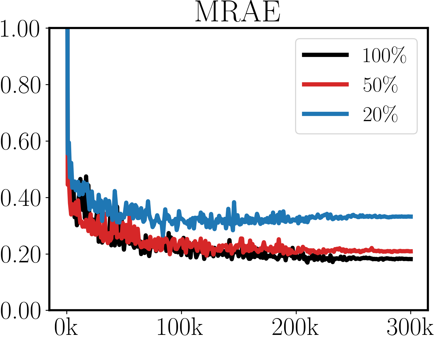
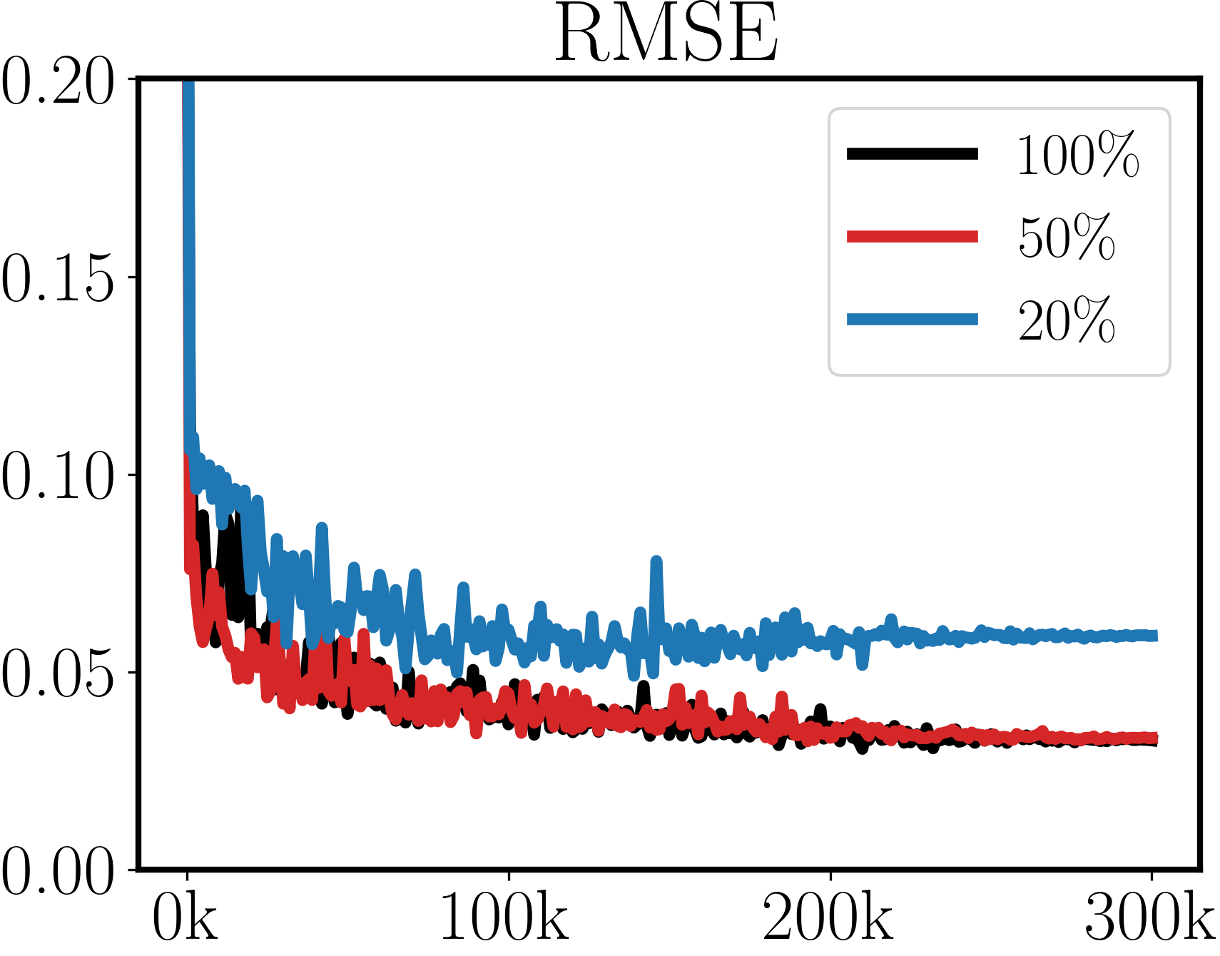
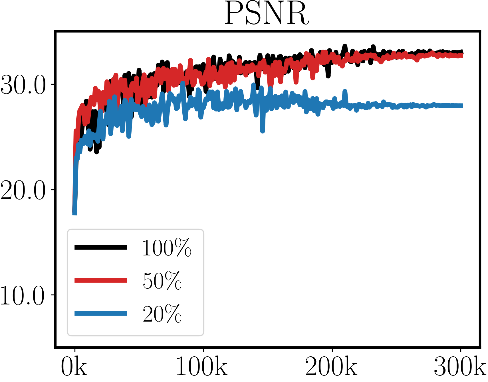
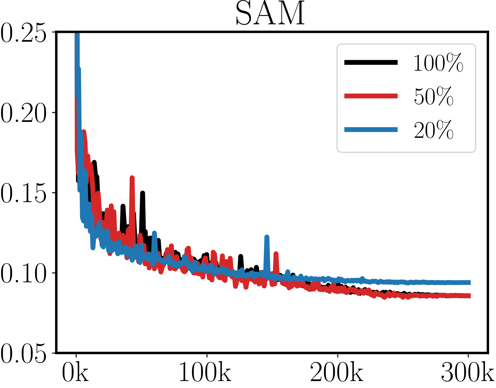
MST-L
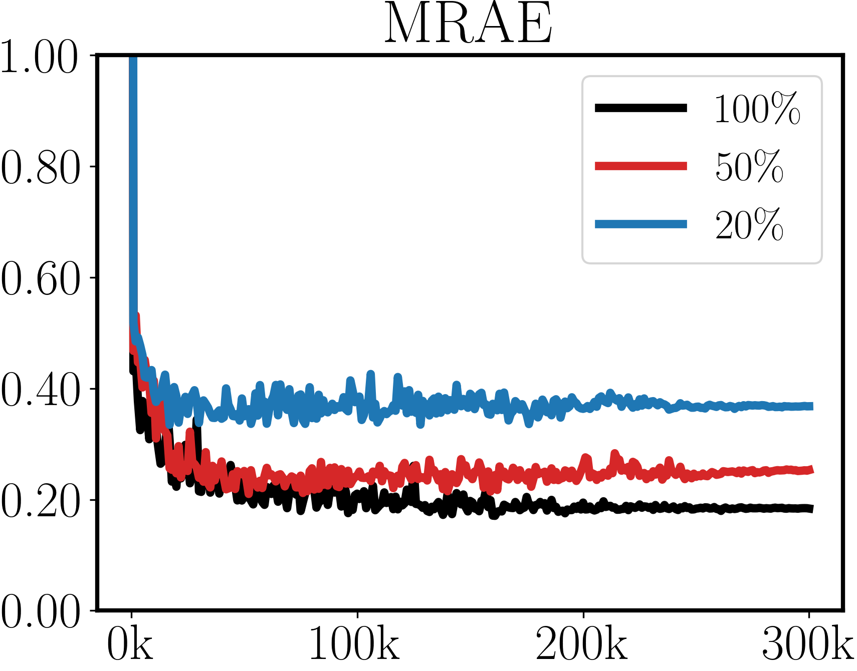
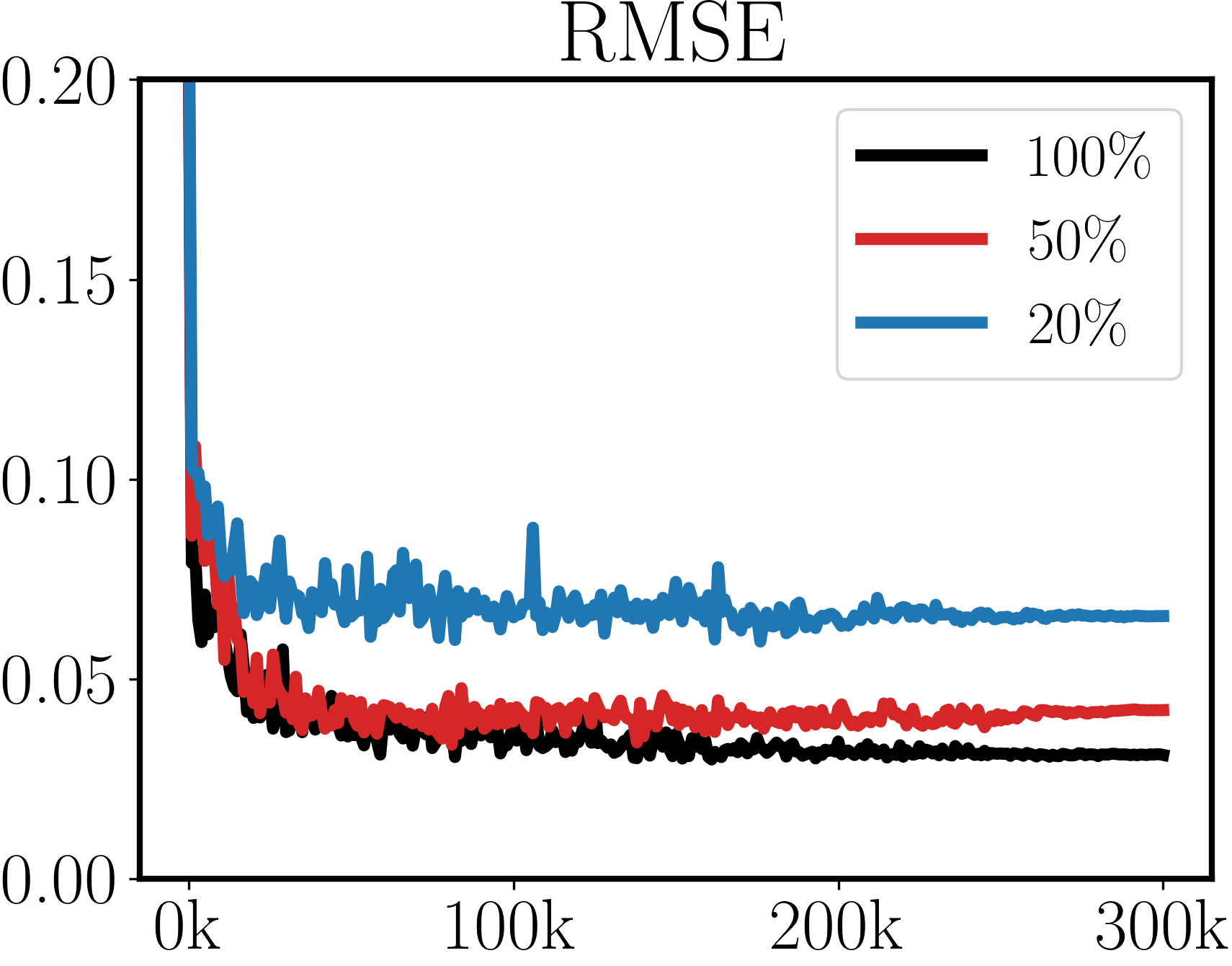
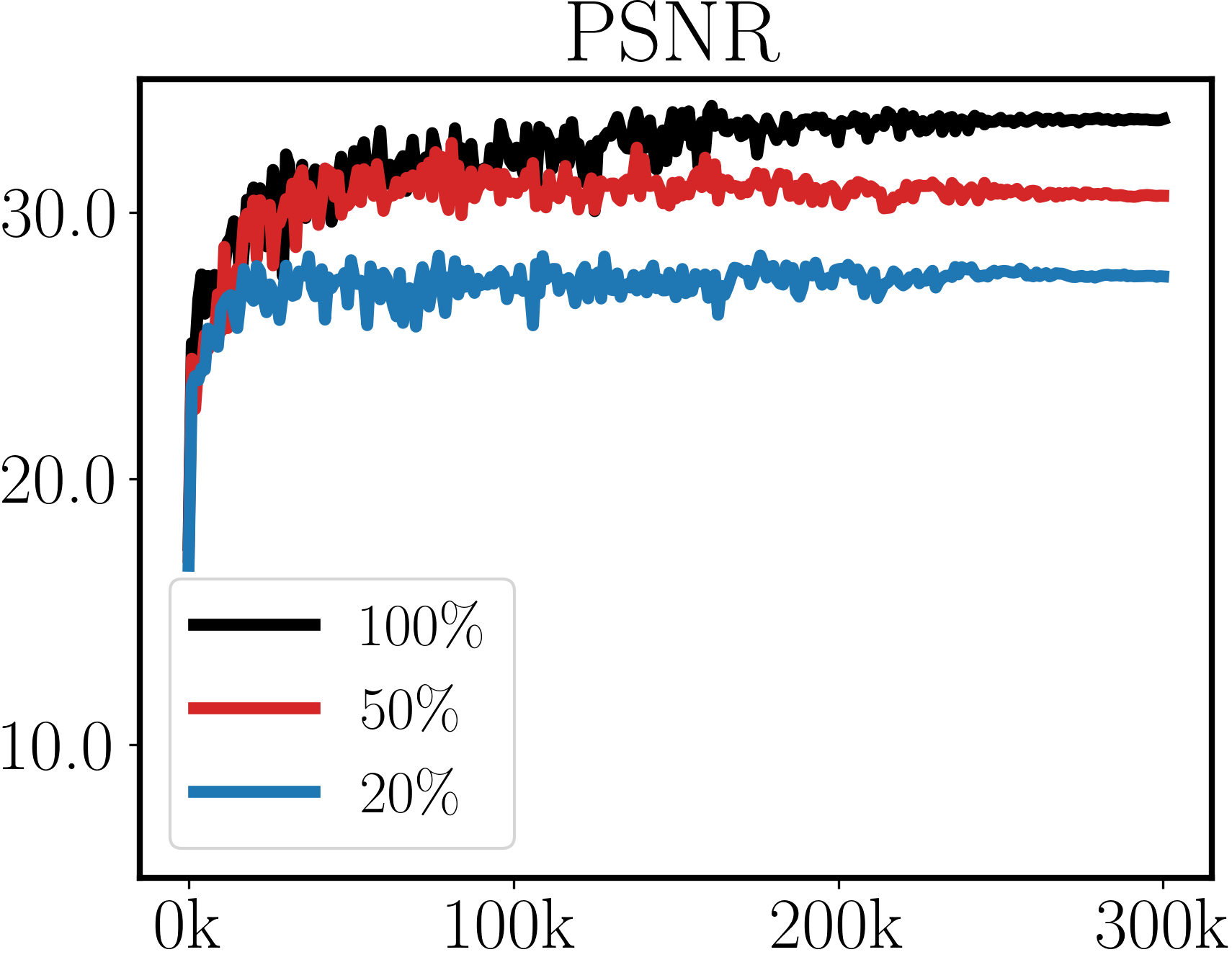
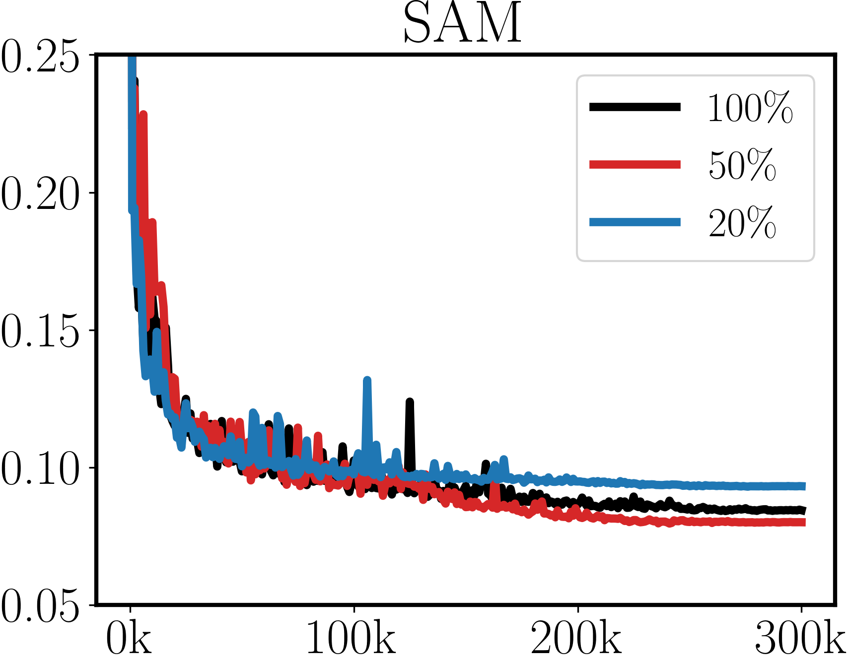
MPRNet
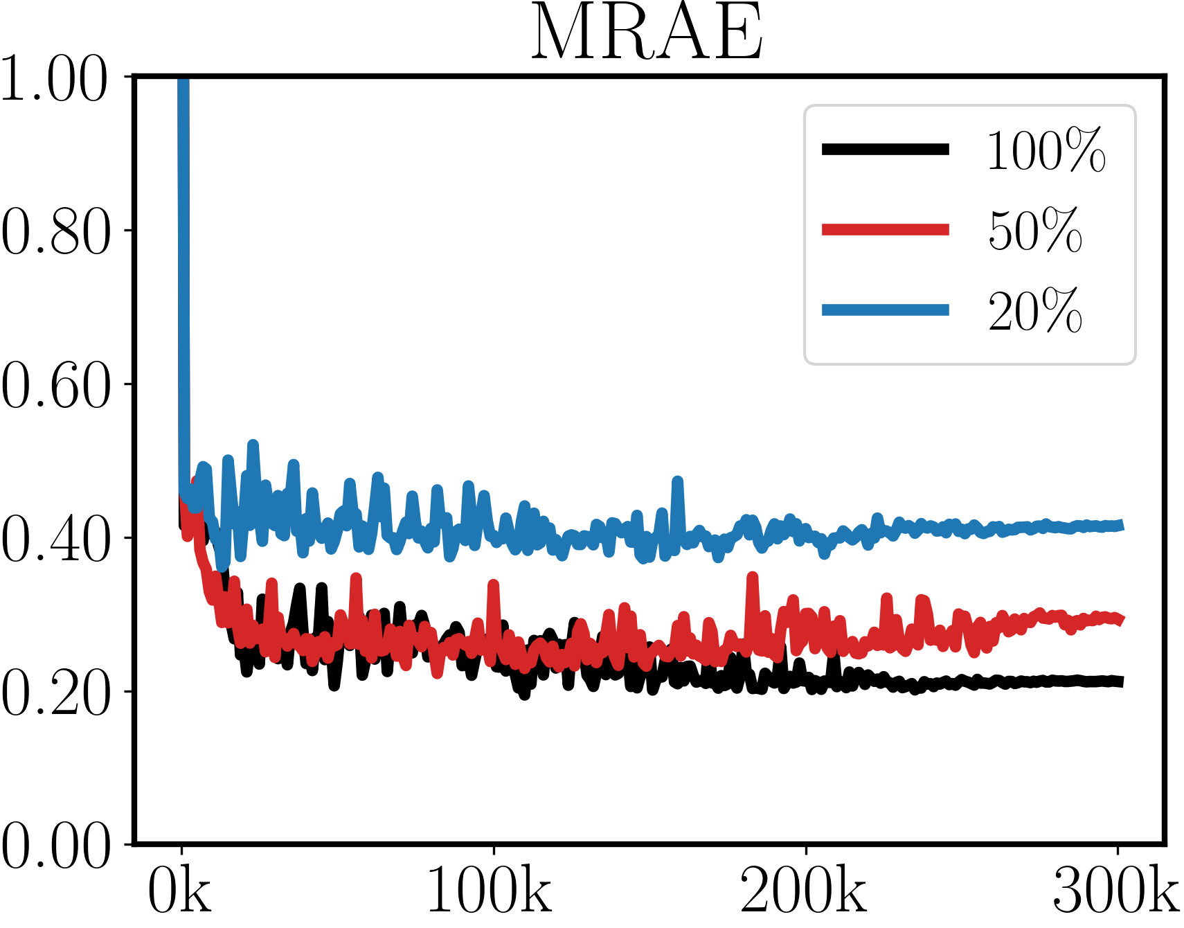
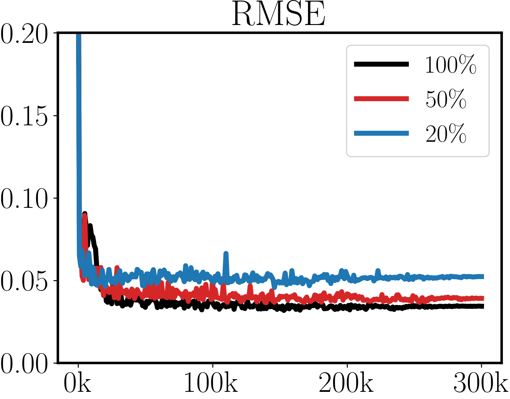
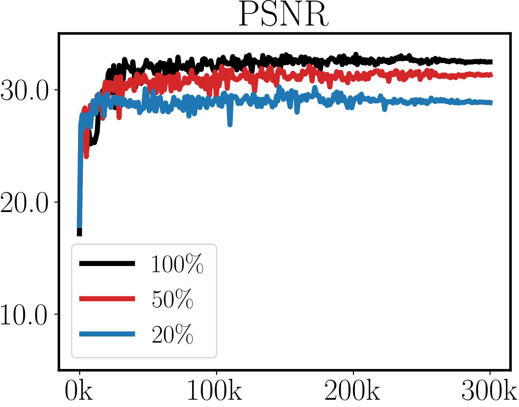
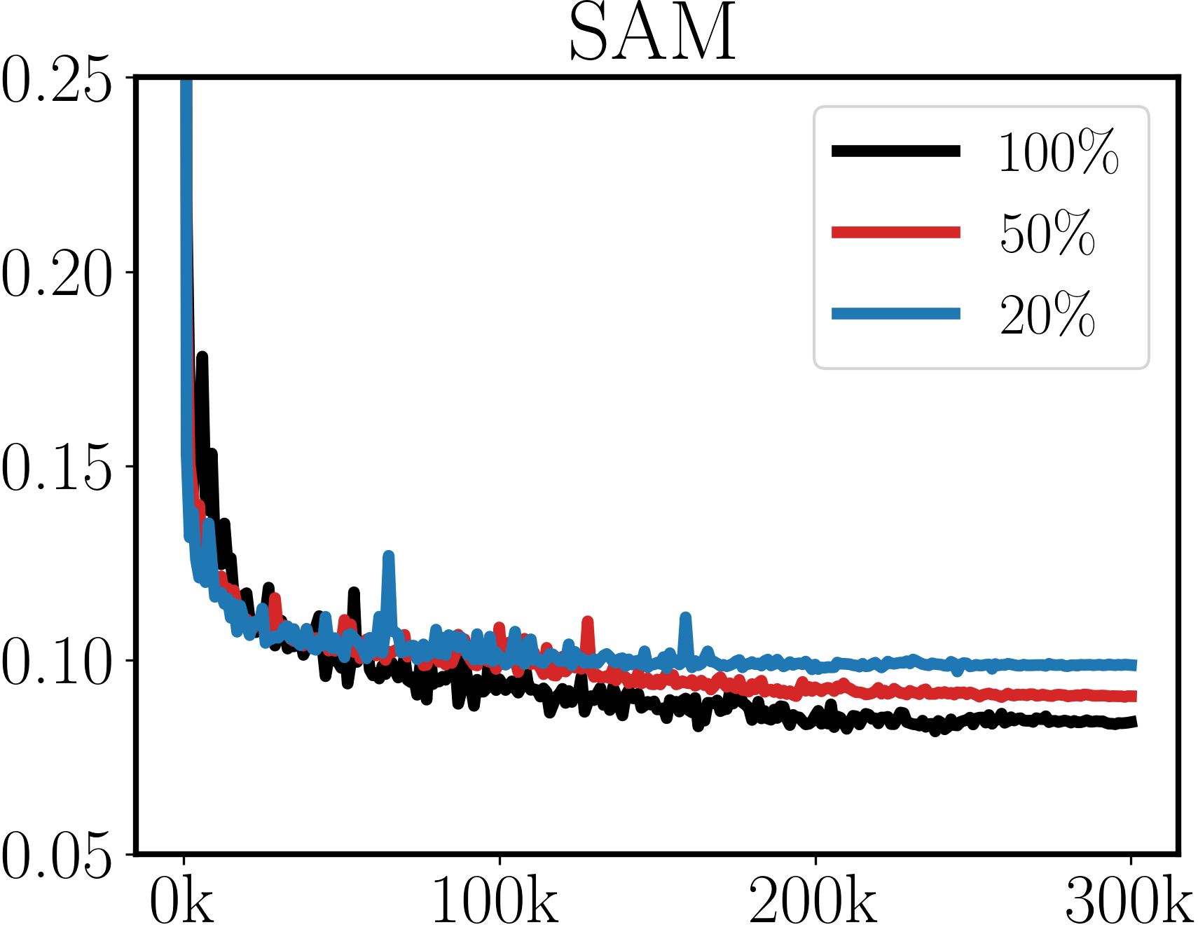
Restormer
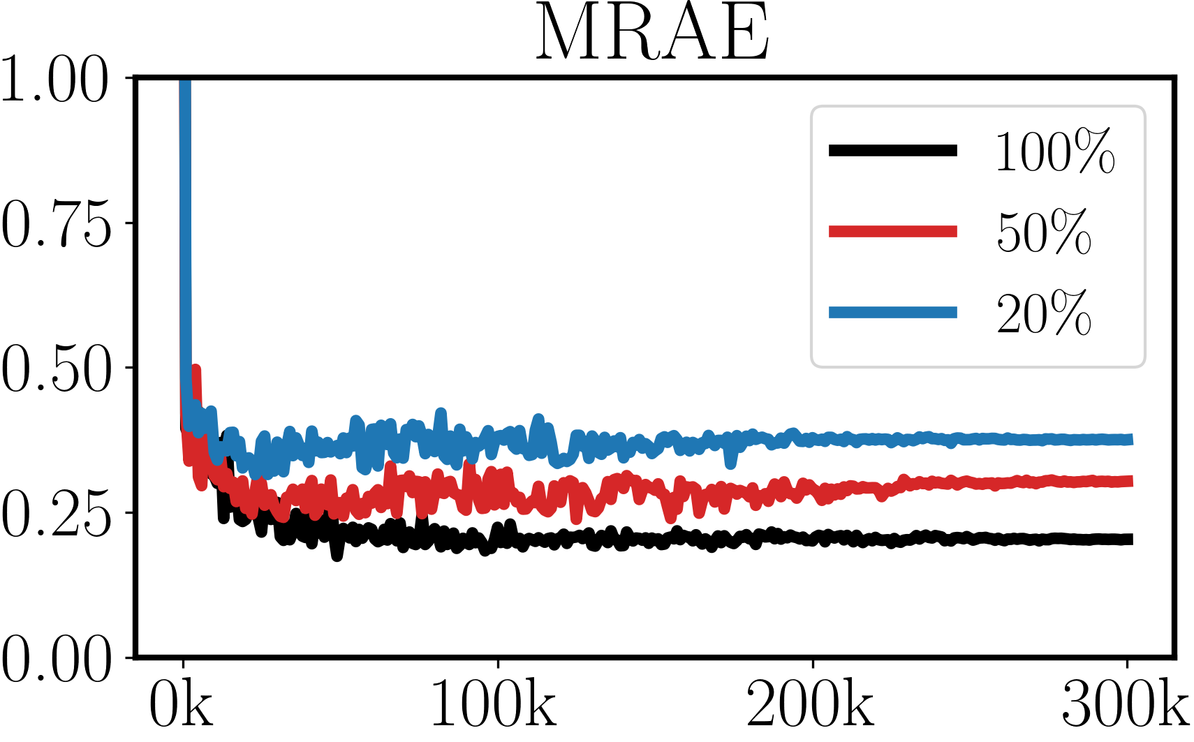
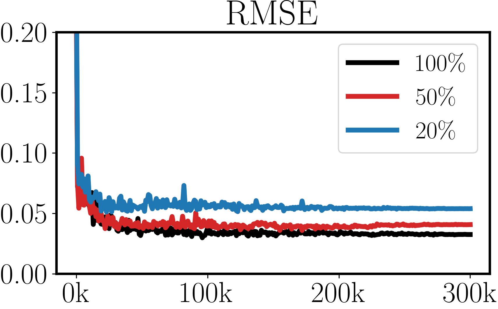
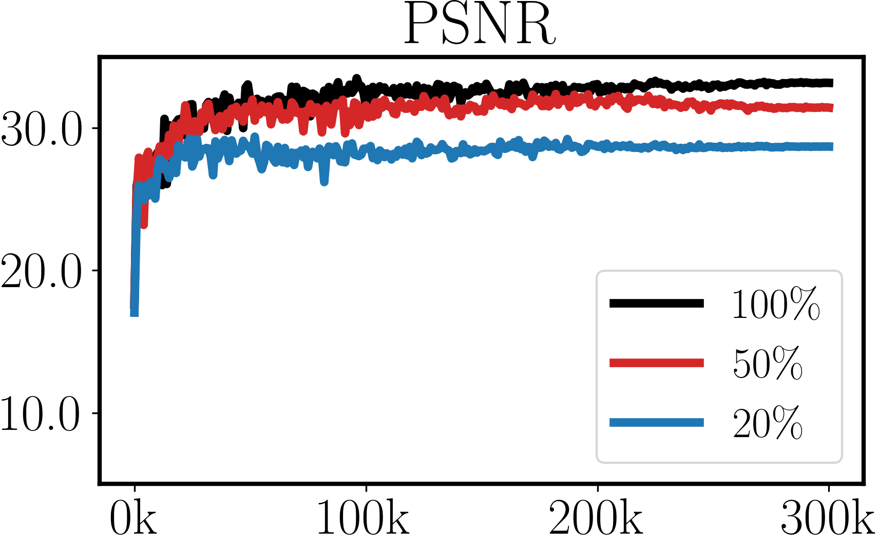
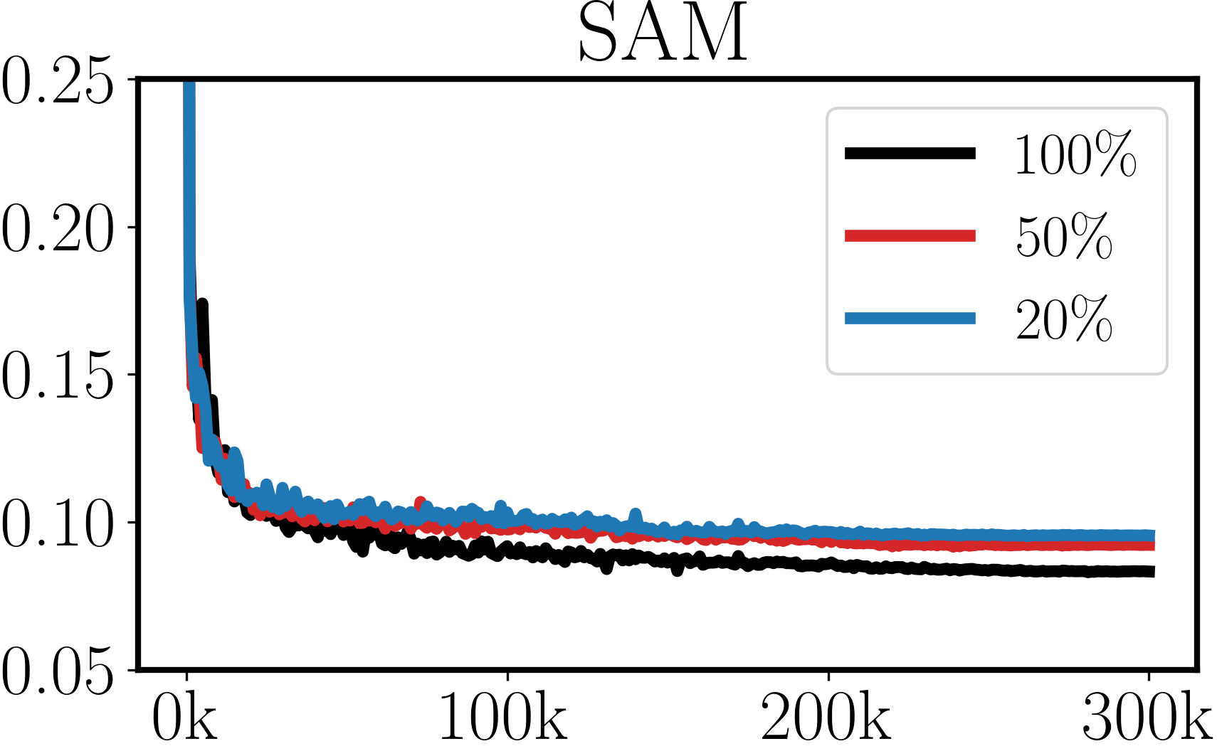
MIRNet
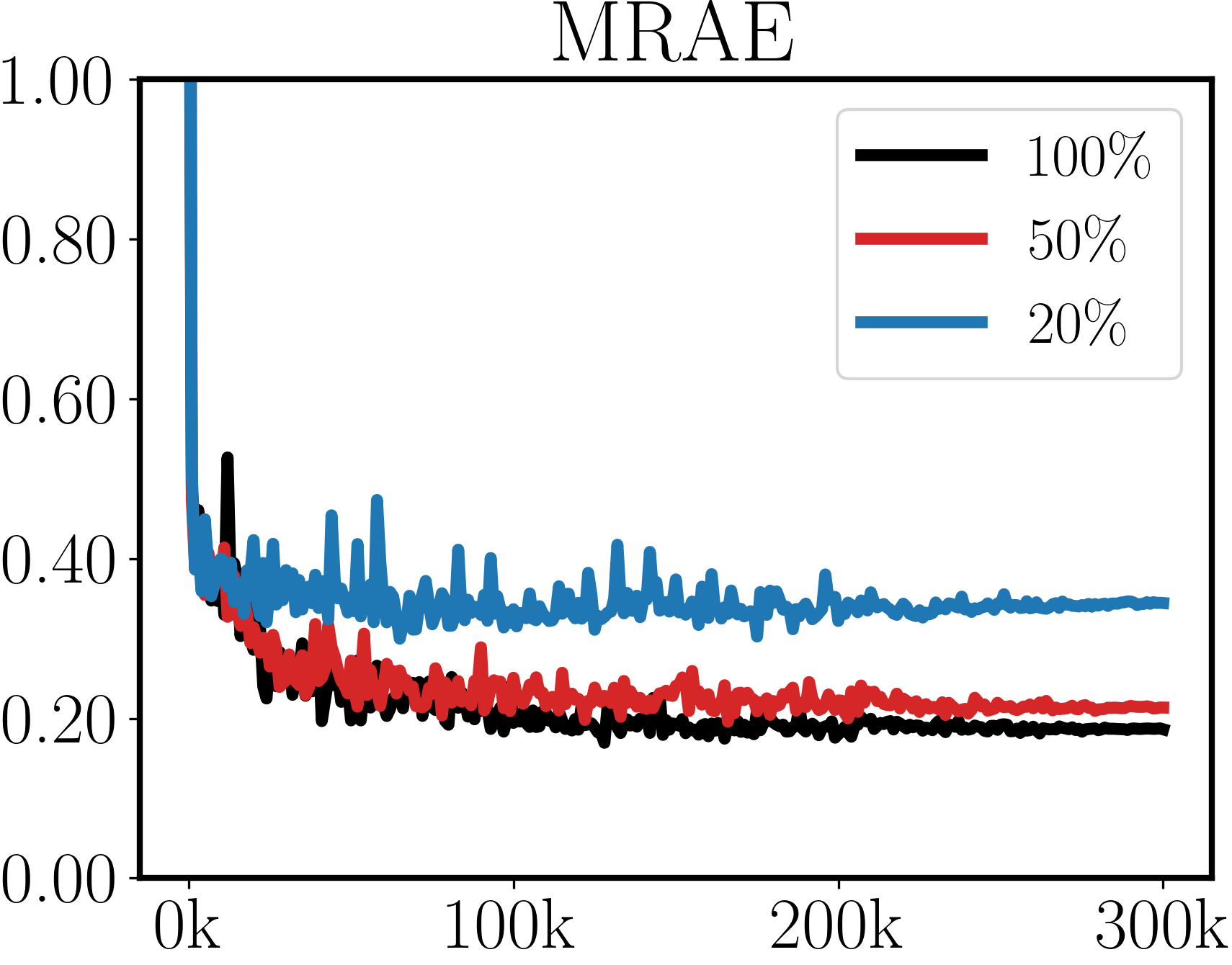
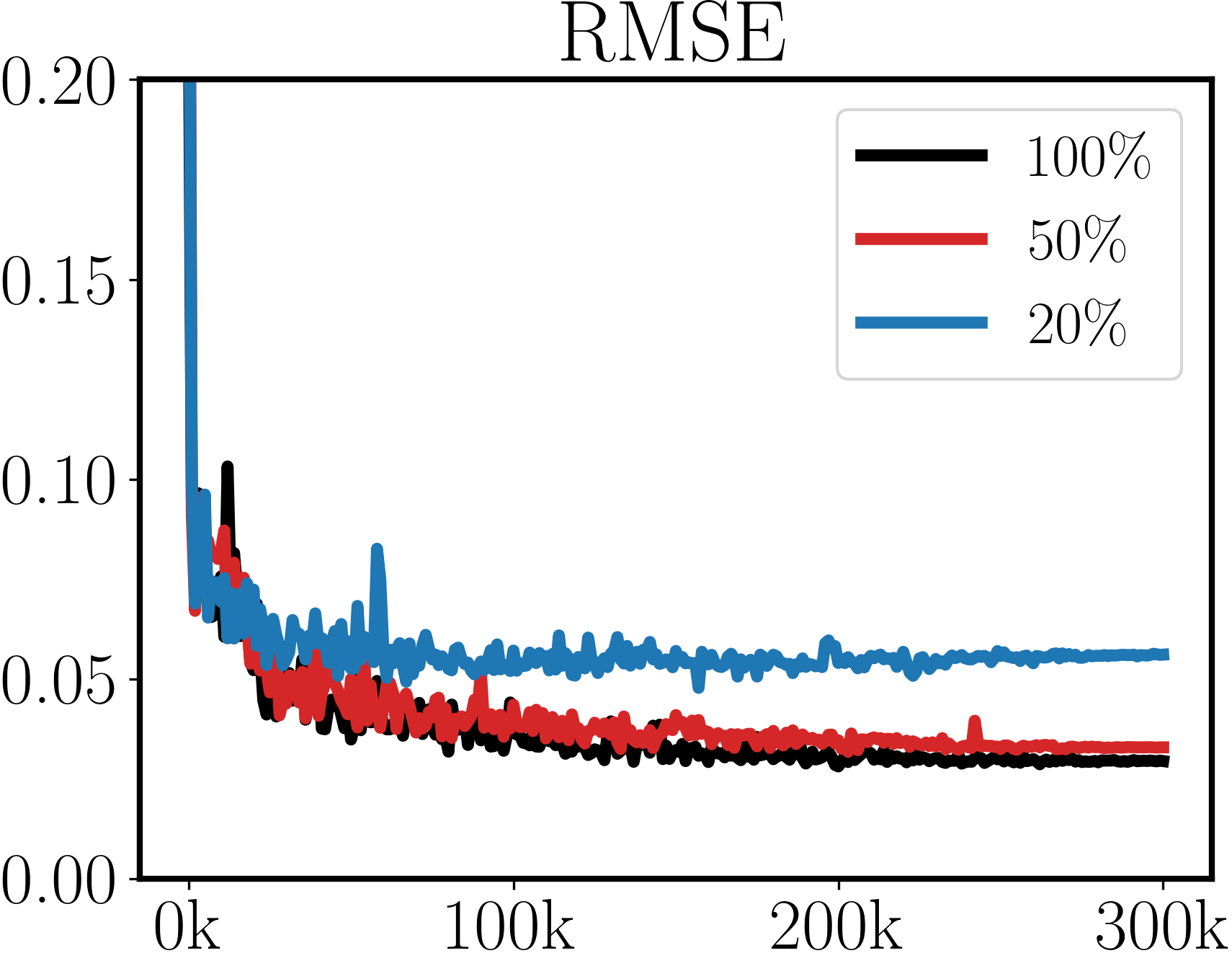
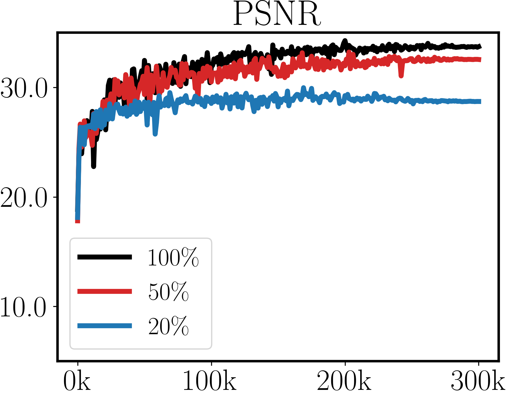
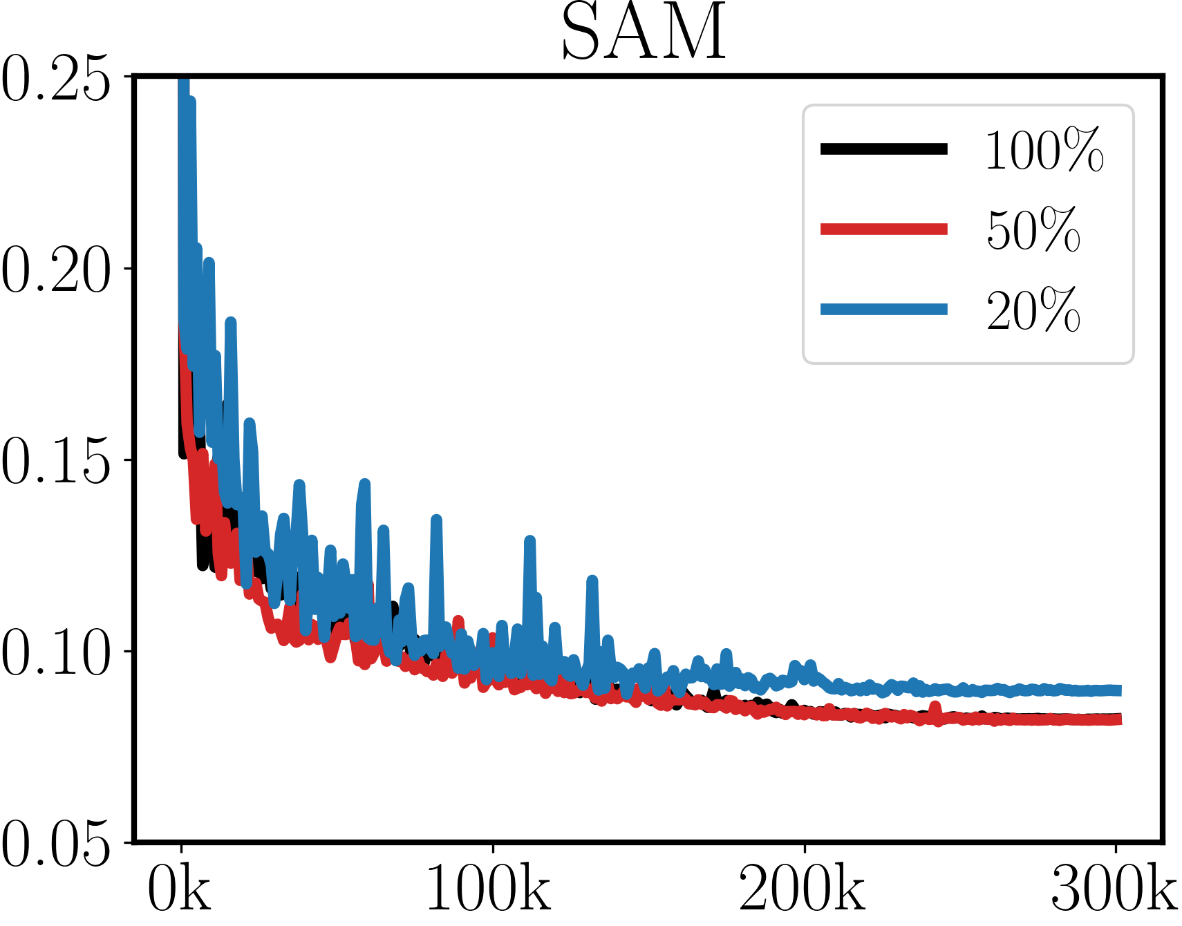
HINet

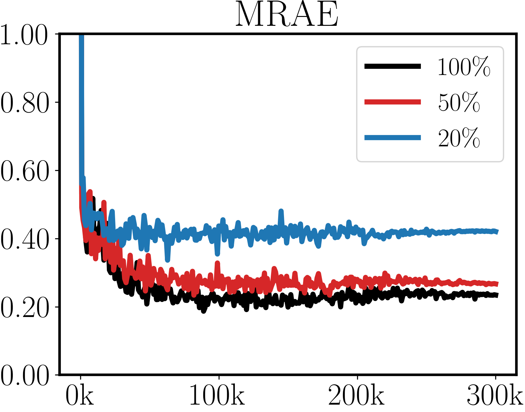
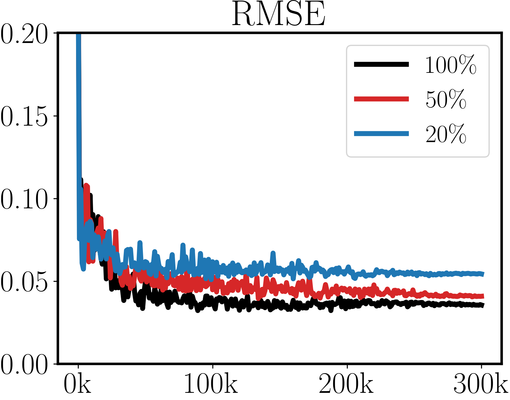
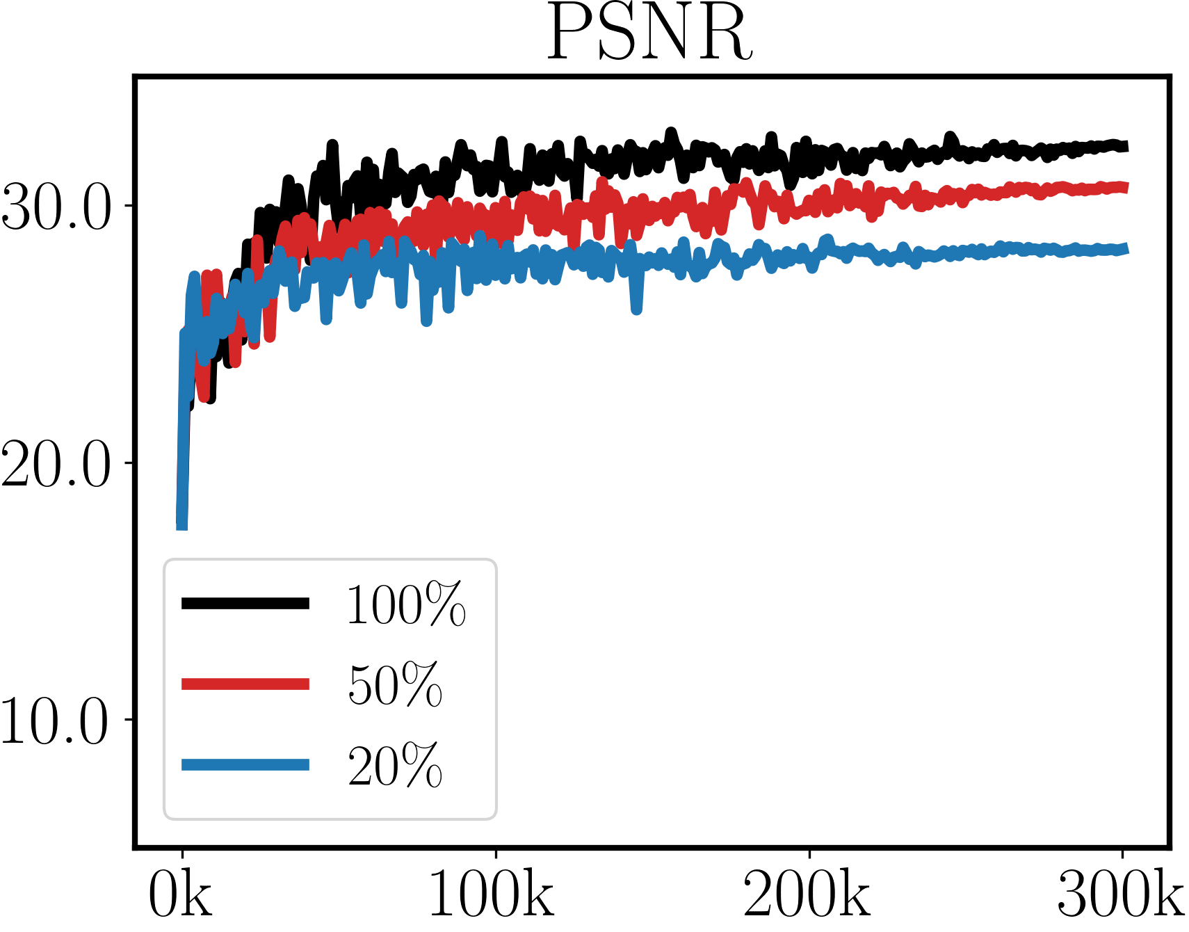
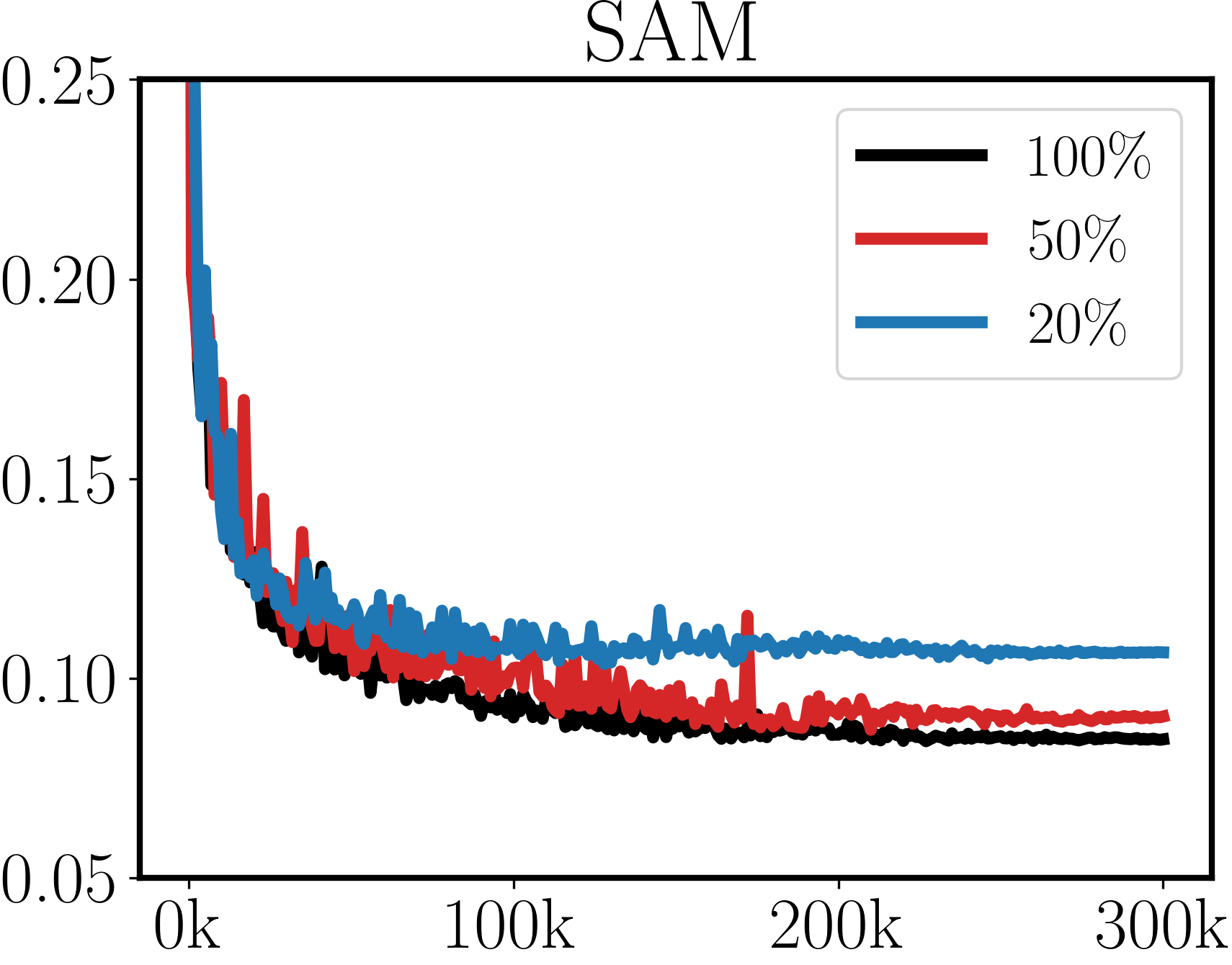
Figure 7: Validation perfromance on MRAE, RMSE, PSNR, and SAM for MST++ [13], MST-L [12], MPRNet[64], Restormer[65], MIRNet[63], and HINet[16] with 100%, 50%, and 20% of the original training data on the ARAD1K dataset.

HDNet
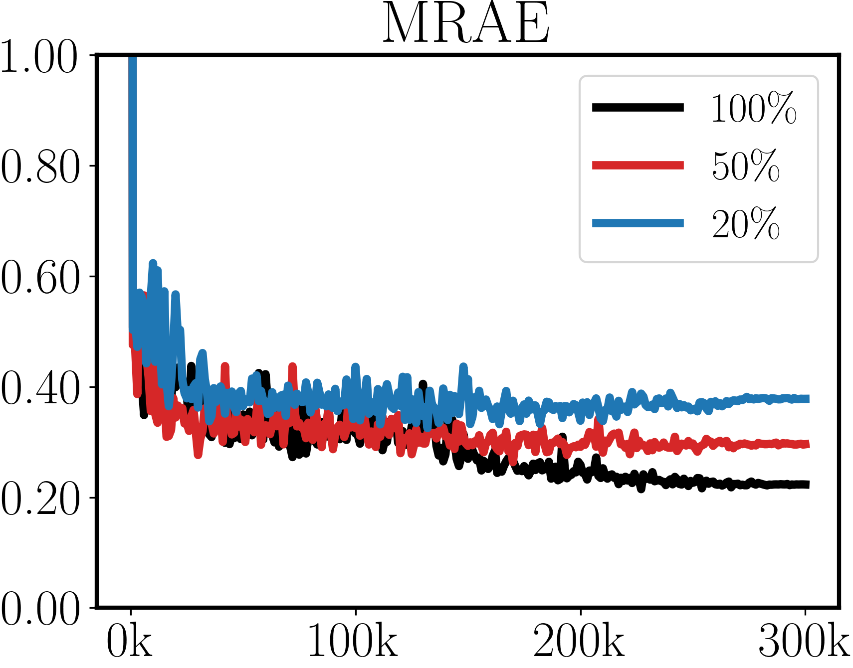
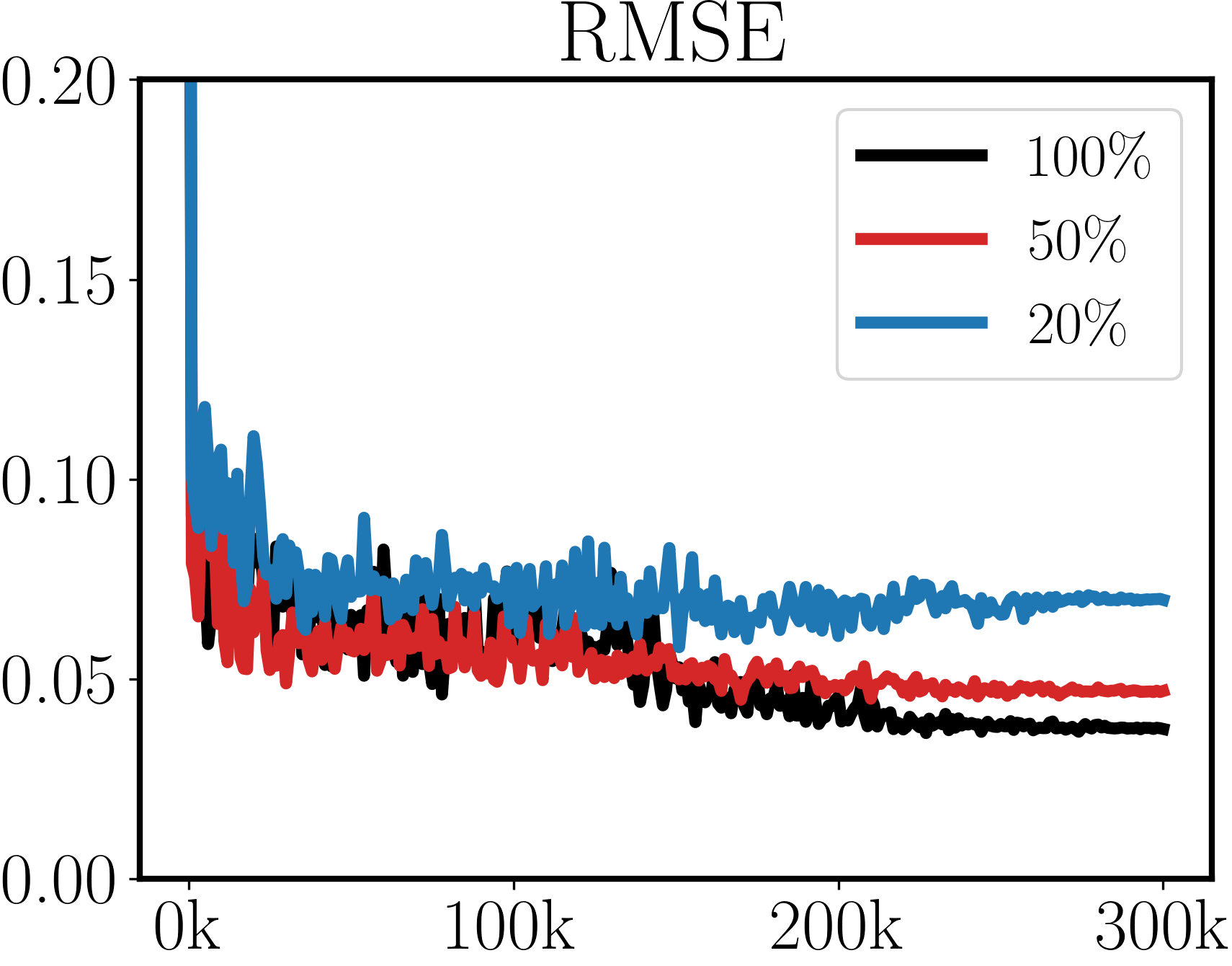
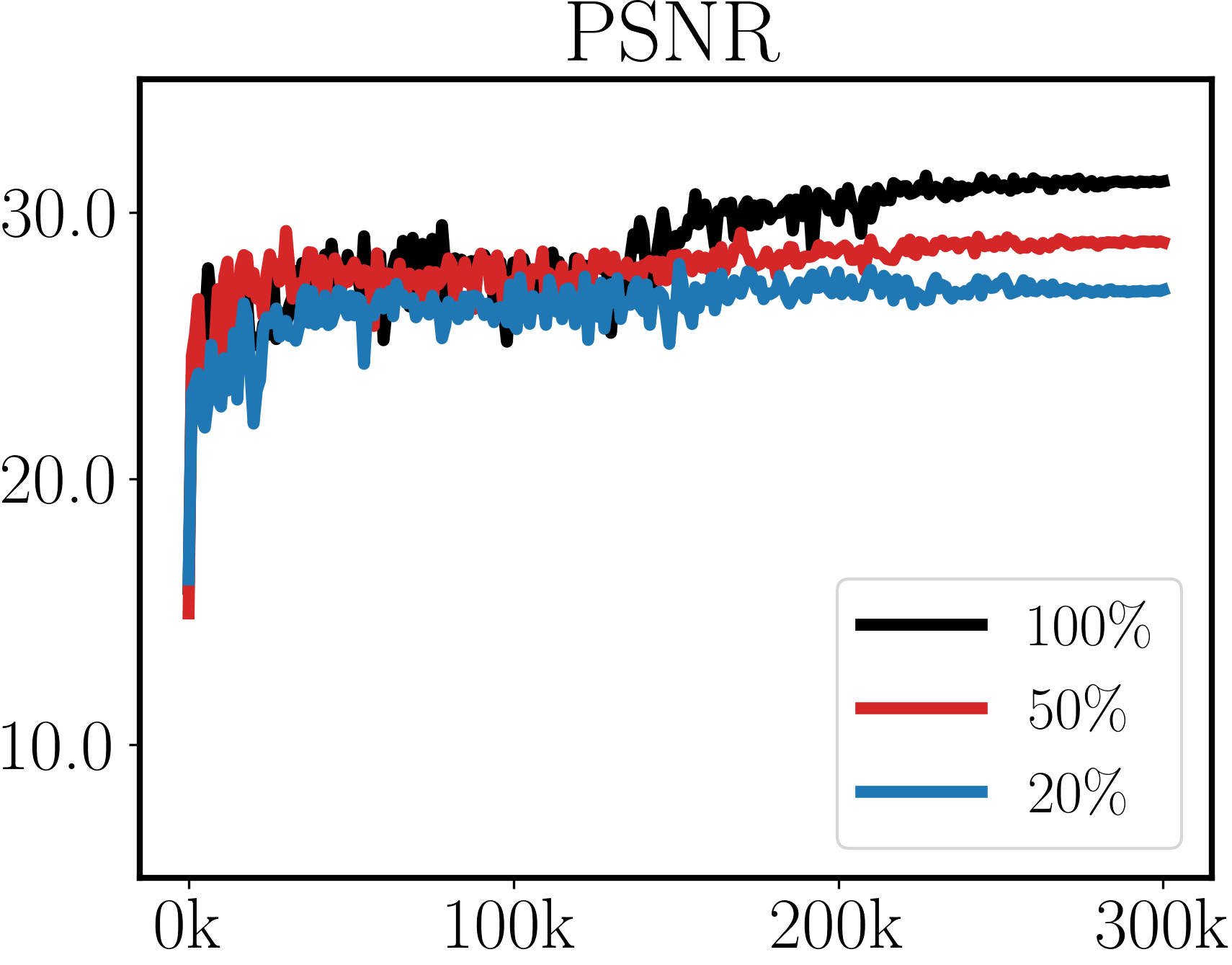
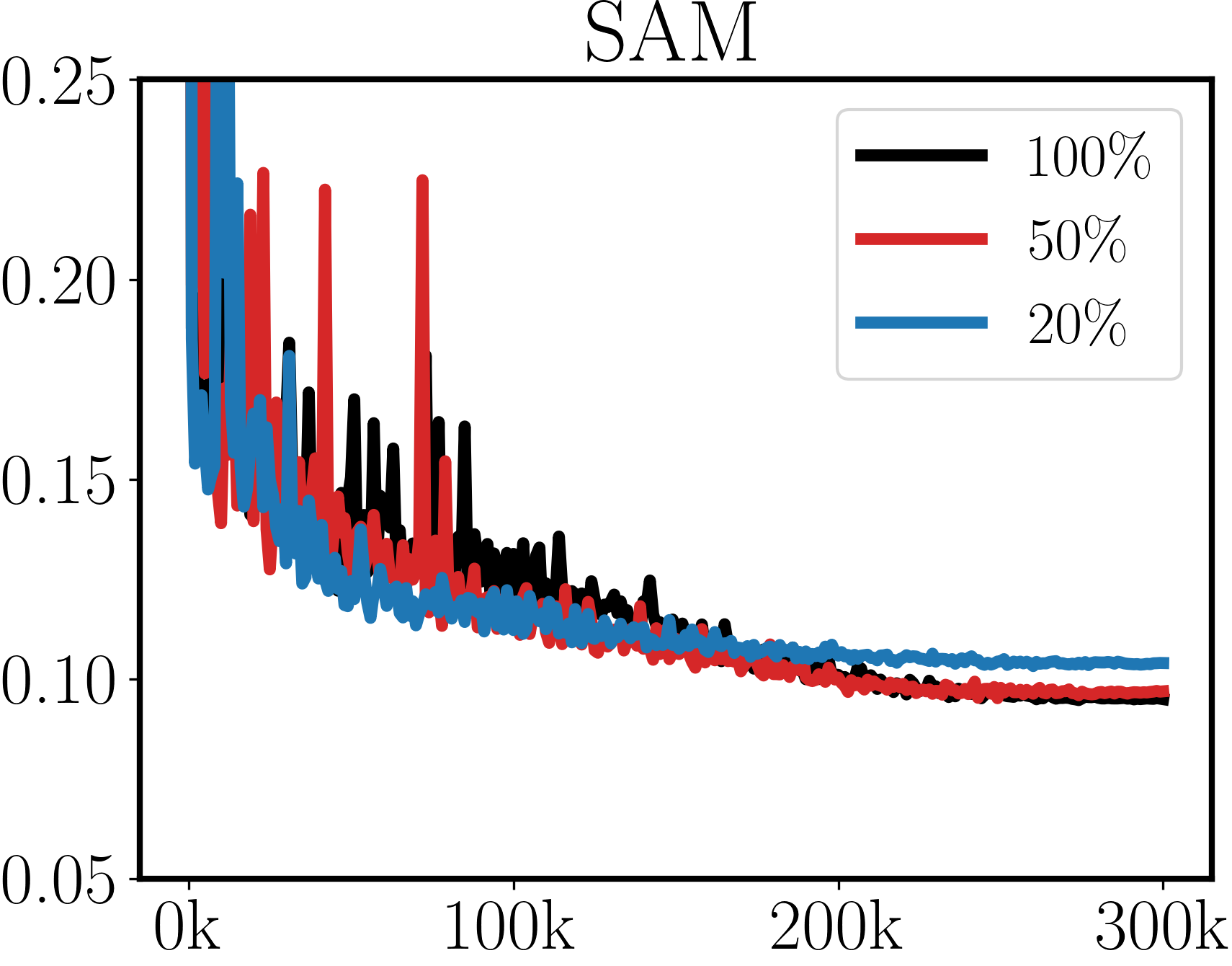
AWAN
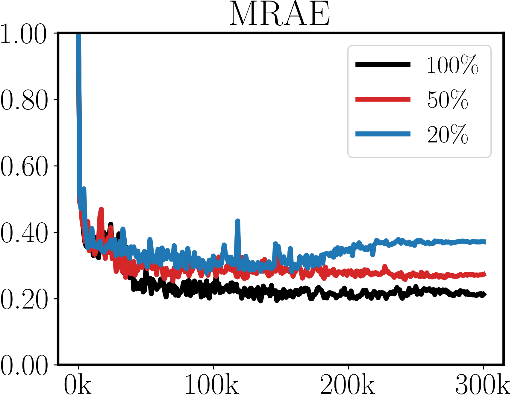
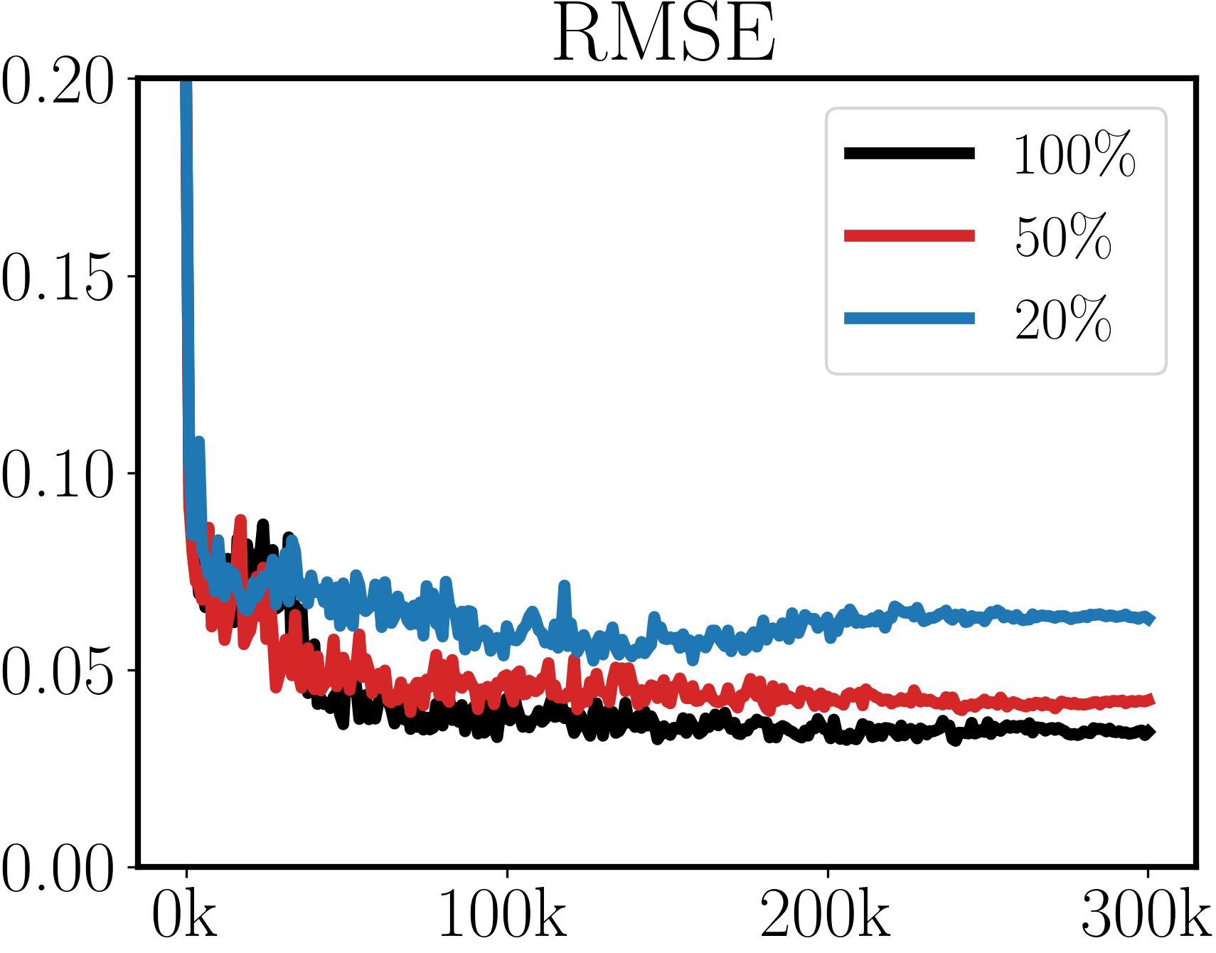
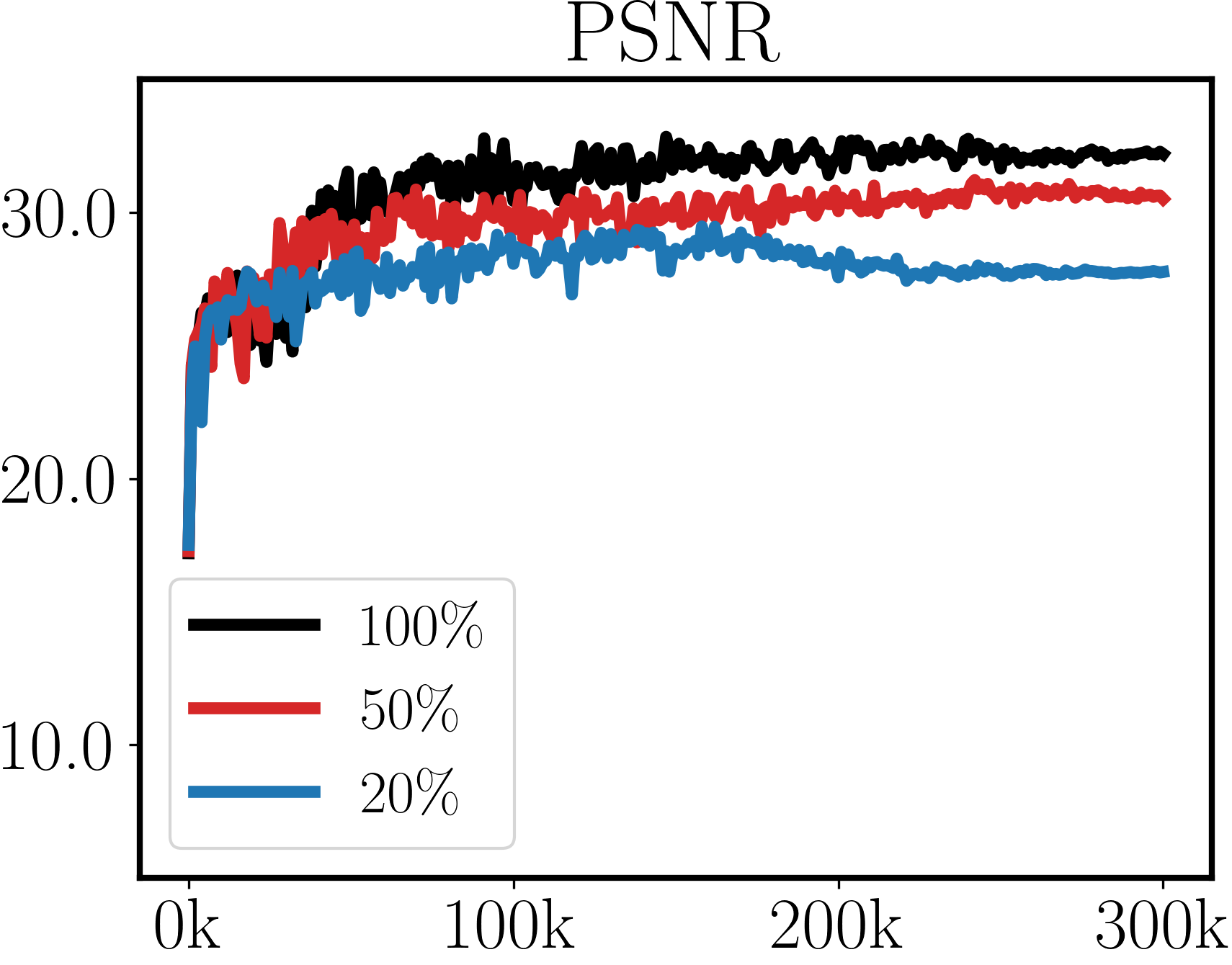
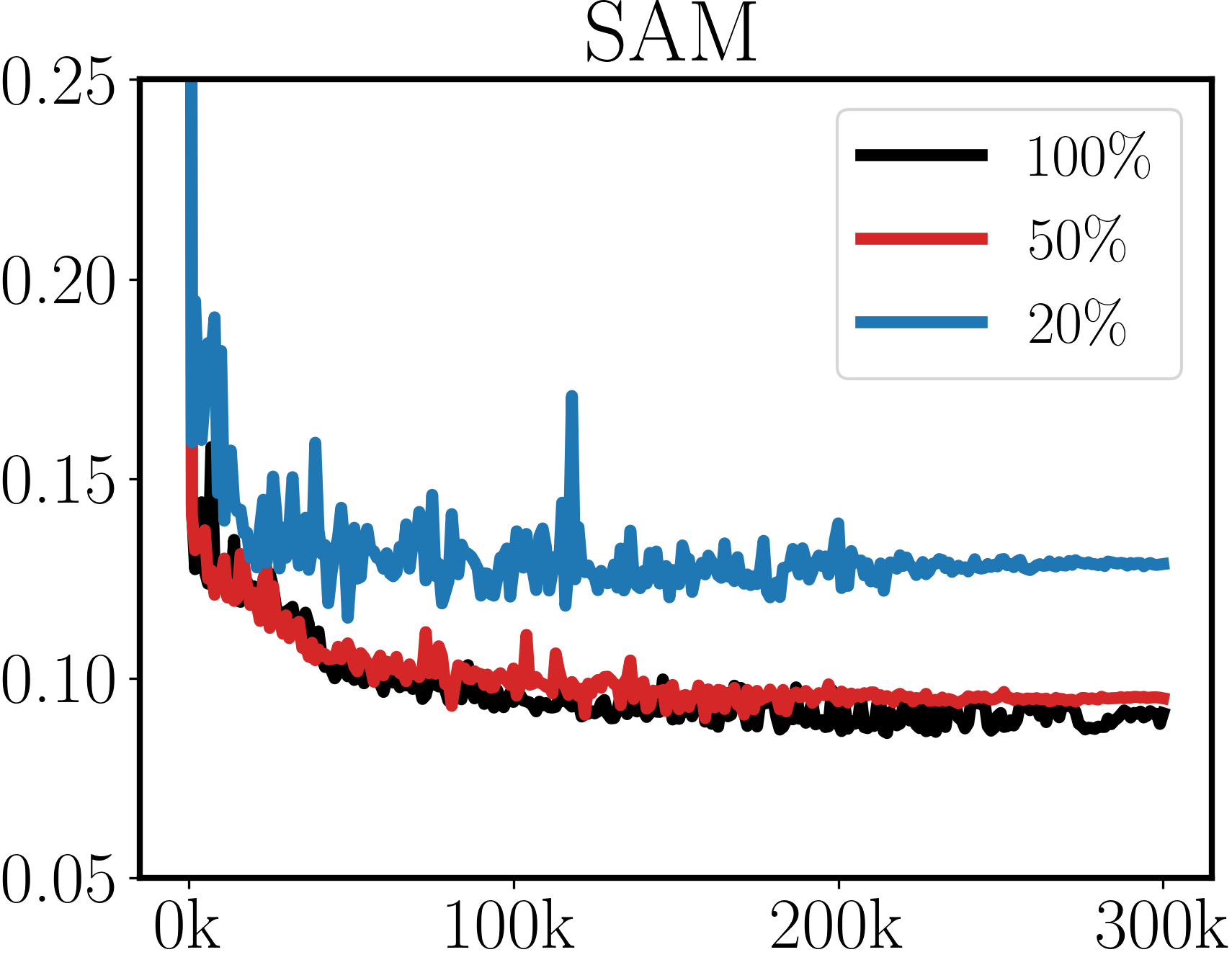
EDSR
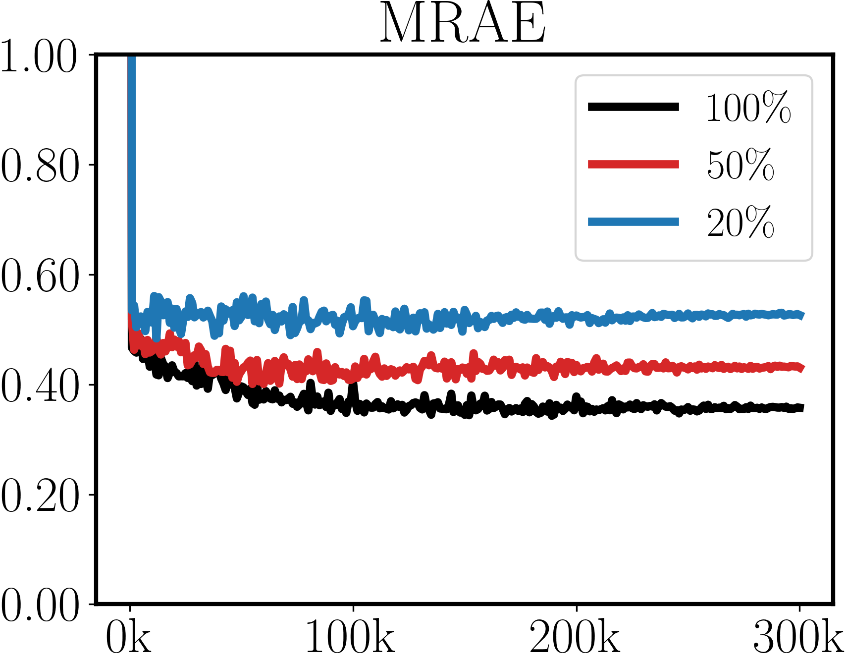
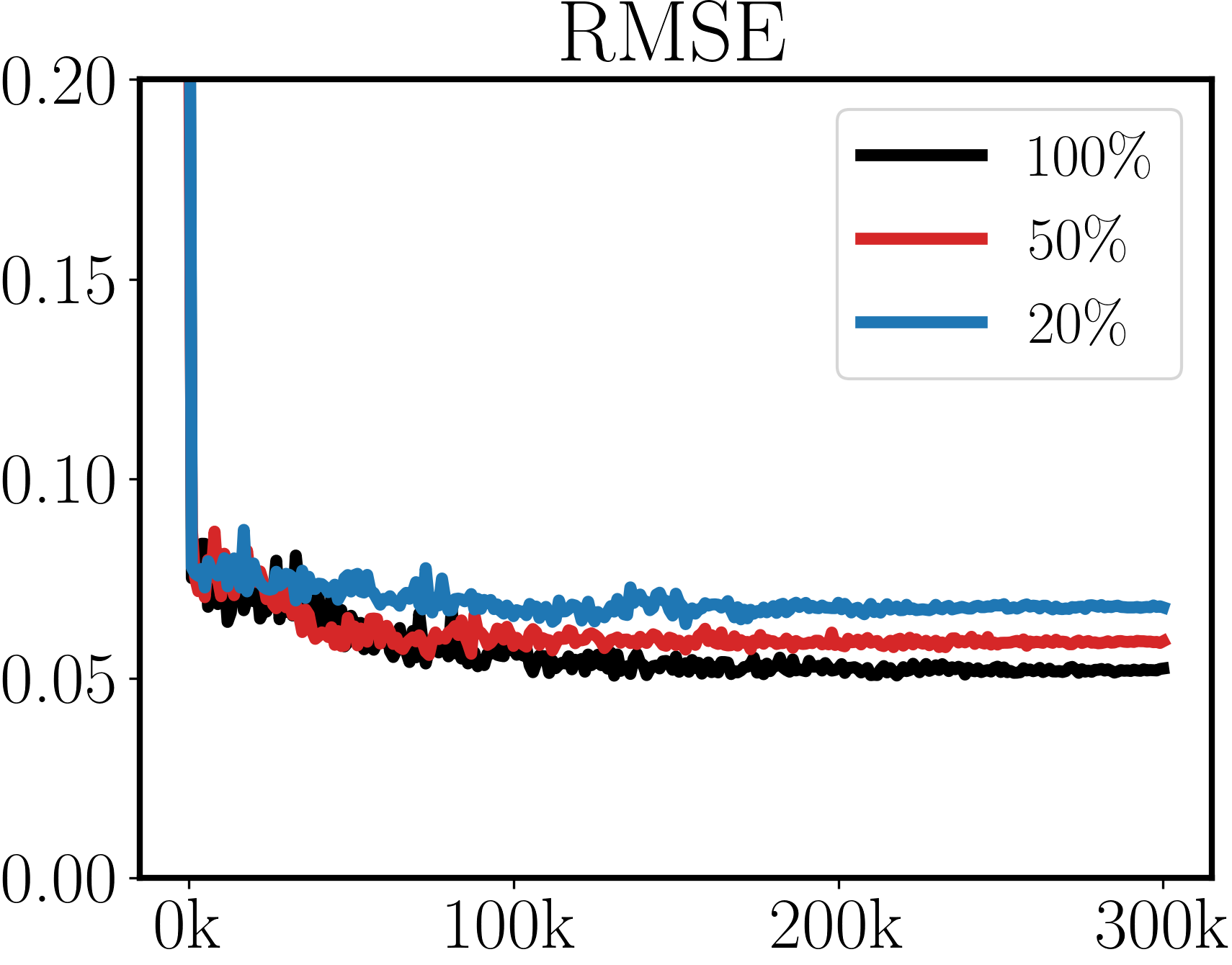
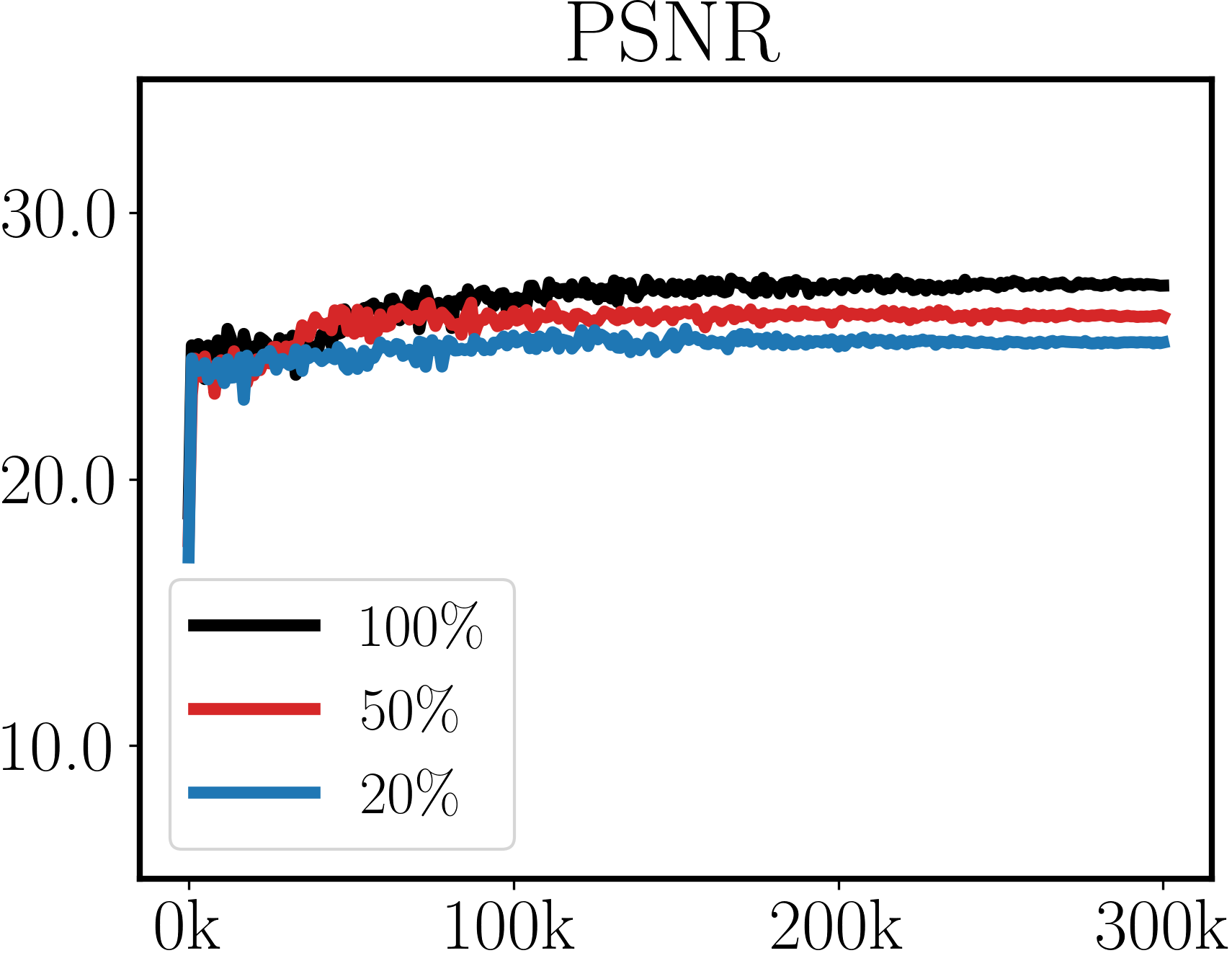
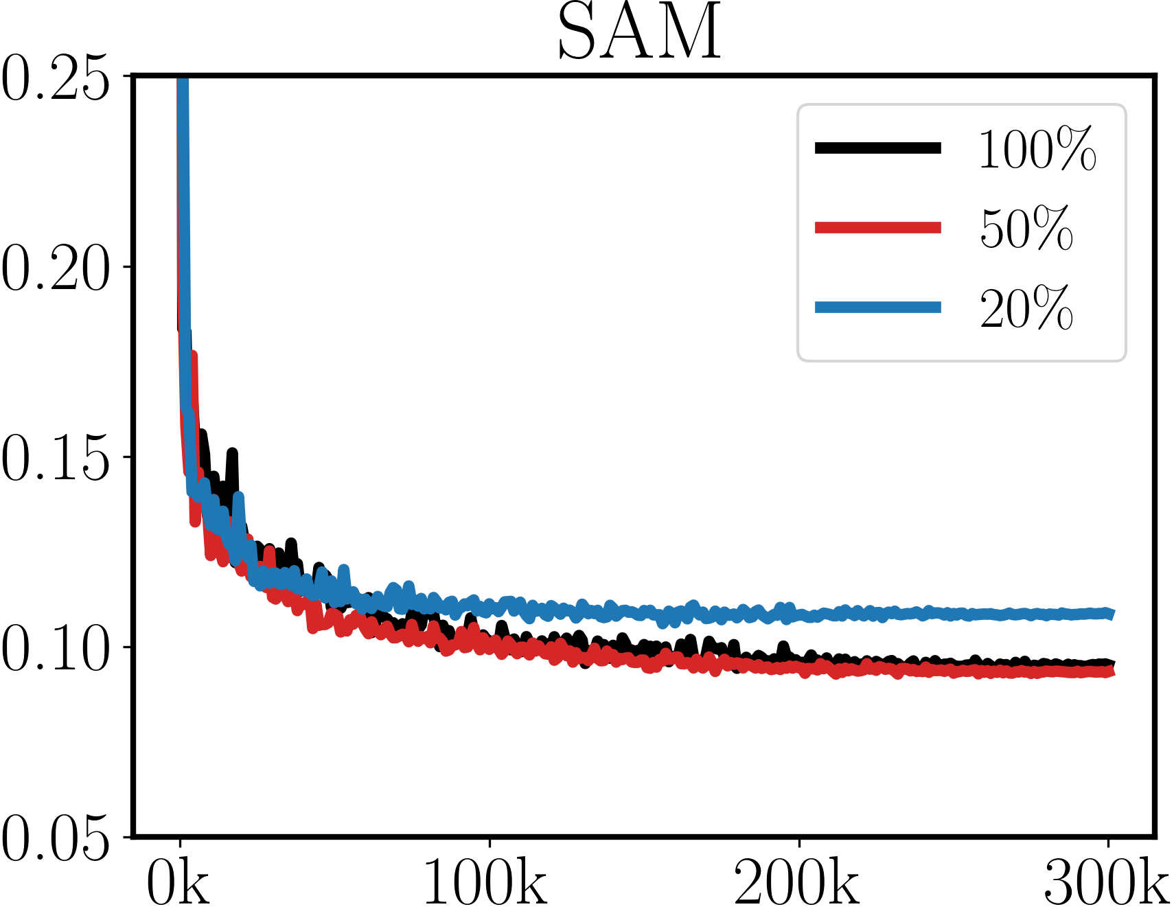
HRNet
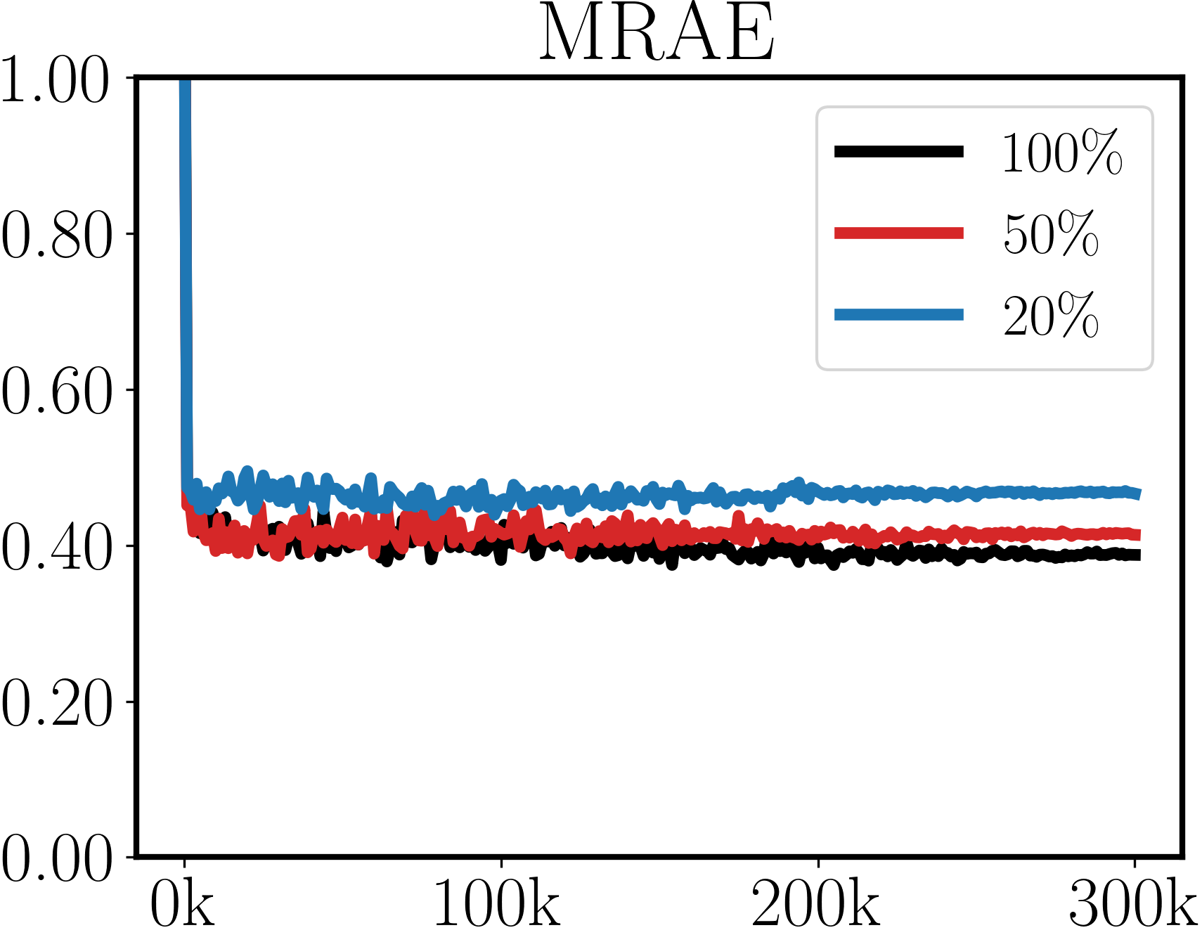
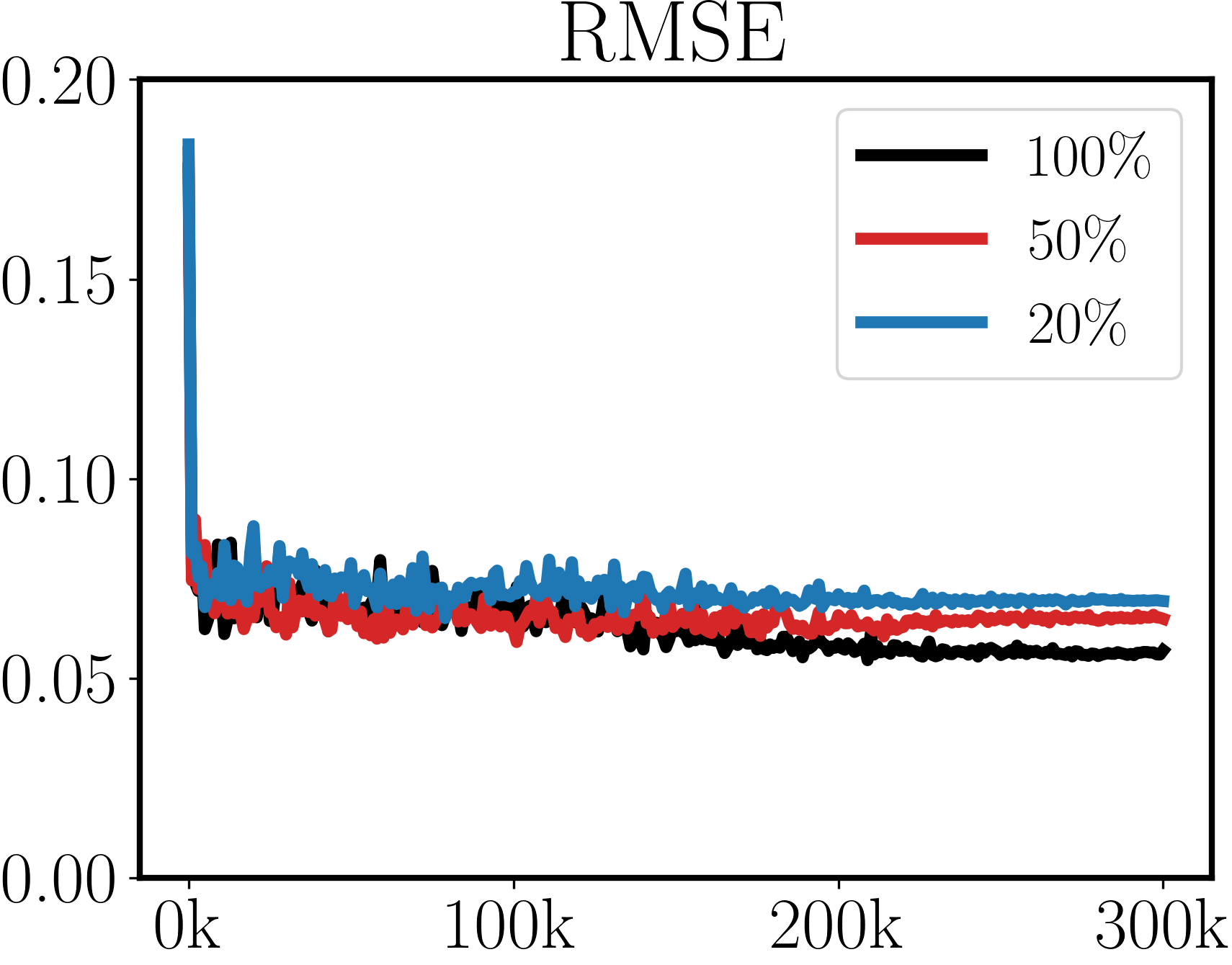
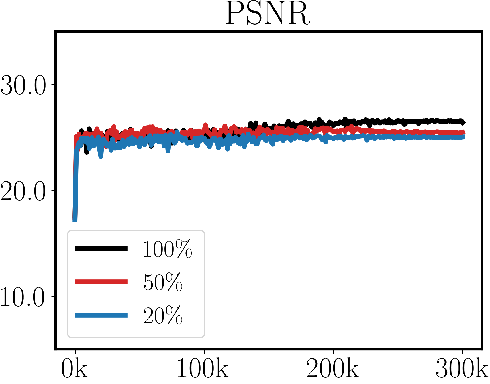
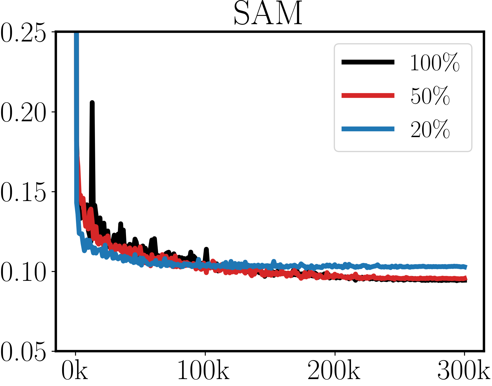
HSCNN+

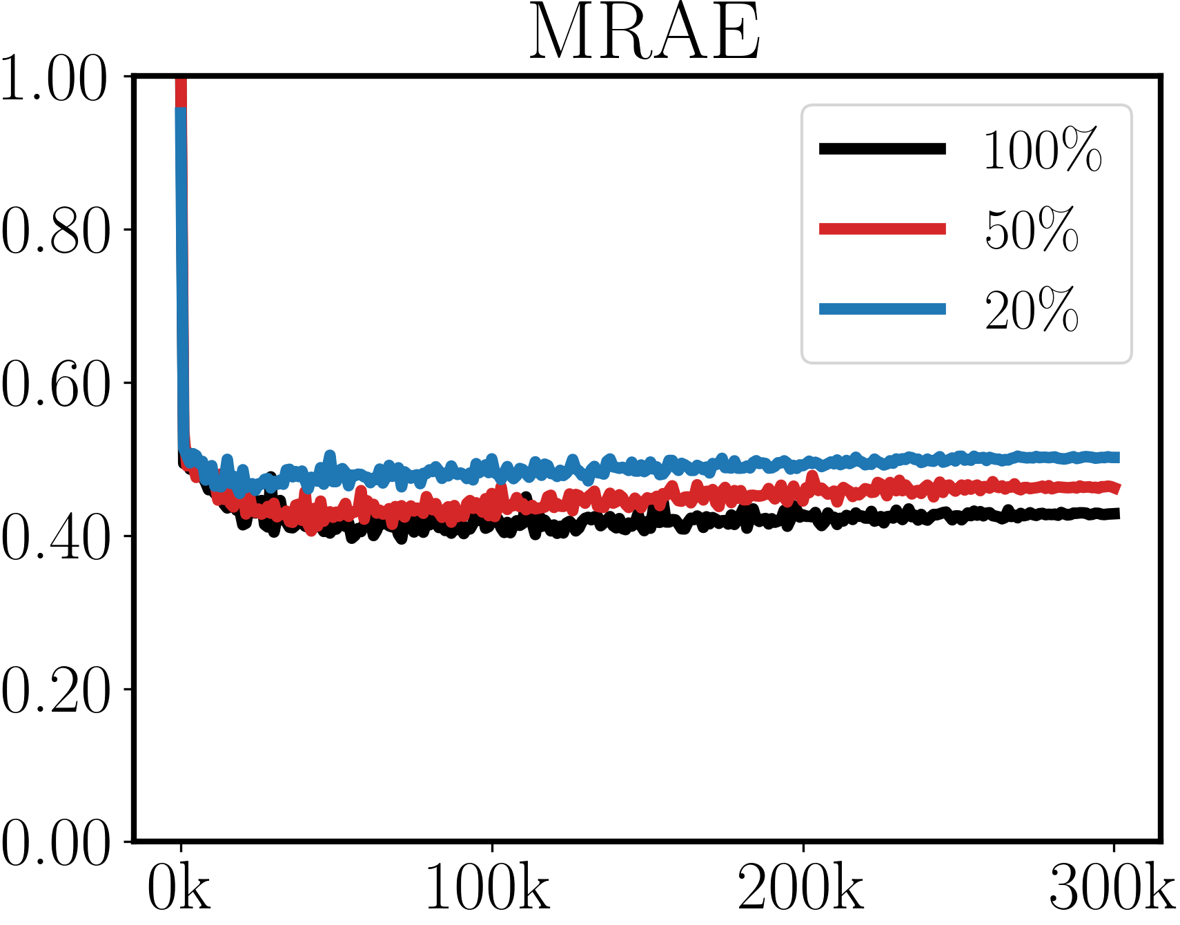
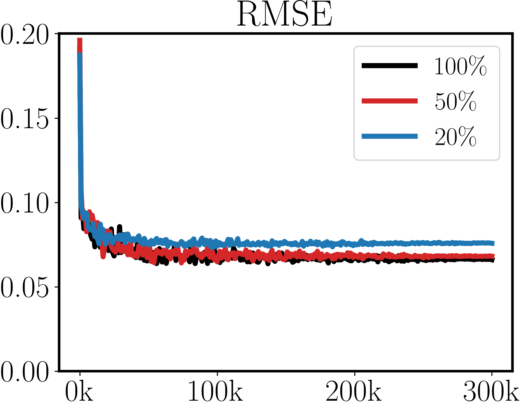
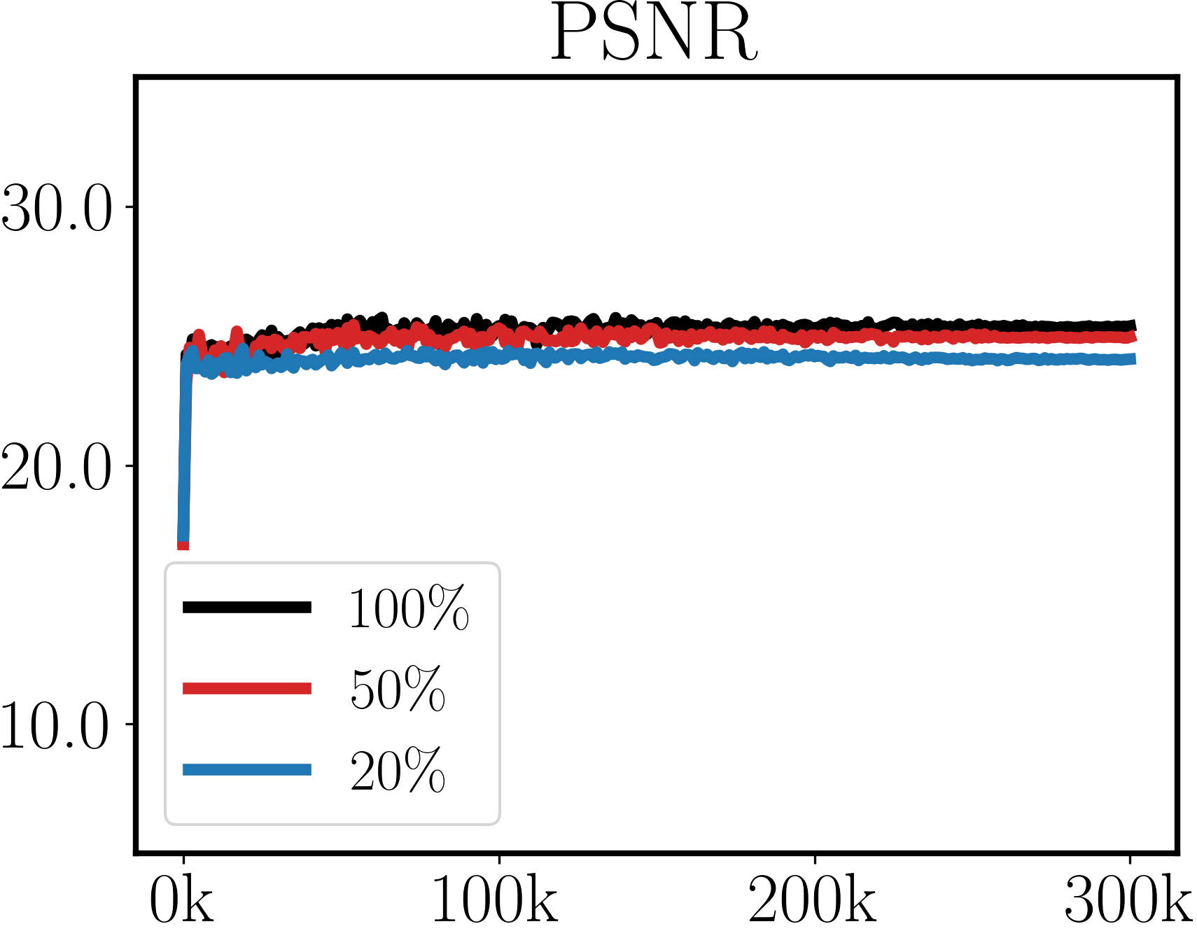
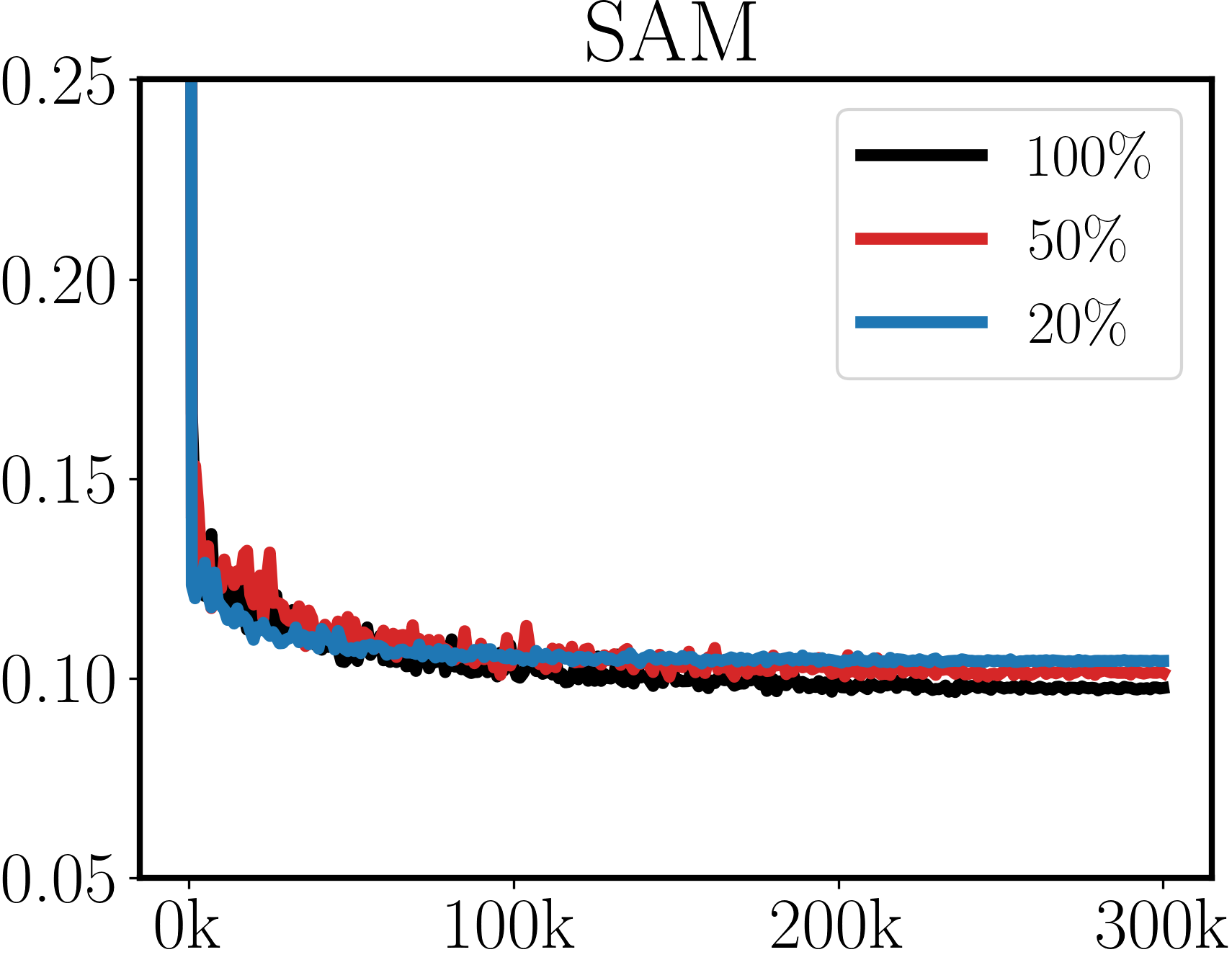
Figure 8: Validation perfromance on MRAE, RMSE, PSNR, and SAM for HDNet[30], AWAN[38], EDSR[40], HRNet[67], and HSCNN+[50] with 100%, 50%, and 20% of the original training data on the ARAD1K dataset.

12 Results of Validation with Unseen Data for Other Networks

In Table 3 of the main paper, we demonstrate the performance drop behaviour of the MST++ network on the ARAD1K dataset. To prove that this is true to other networks as well, we carry out the same experiments for all the other candidate networks. The results are summarized in Supplemental Table LABEL:tab:supp_validation_ARAD1K. As the noise levels, RGB formats, and aberration conditions asymptotically approach realistic imaging scenarios in the real world, the pre-trained models [13] for other networks gradually degrade, similar as the MST++. All the results consistently support our conclusion about the generalization difficulties of these methods in realistic imaging conditions.

Network	Data property				MRAE $\downarrow$	RMSE $\downarrow$	PSNR $\uparrow$	SAM $\downarrow$
	Data source	Noise (npe)	RGB format	Aberration
MST++	NTIRE 2022	unknown	jpg (Q unknown)	None	0.170	0.029	33.8	0.084
	Synthesized	0	jpg (Q = 65)	None	0.460	0.049	29.2	0.094
		0	png (lossless)	None	0.362	0.057	28.7	0.087
		1000	png (lossless)	CA*	0.312	0.055	28.4	0.118
MST-L	NTIRE 2022	unknown	jpg (Q unknown)	None	0.181	0.031	33.0	0.091
	Synthesize	0	jpg (Q = 65)	None	0.417	0.047	29.7	0.099
		0	png (lossless)	None	0.384	0.058	28.4	0.096
		1000	png (lossless)	CA*	0.327	0.055	28.0	0.118
MPRNet	NTIRE 2022	unknown	jpg (Q unknown)	None	0.182	0.032	32.9	0.088
	Synthesize	0	jpg (Q = 65)	None	0.453	0.048	29.1	0.092
		0	png (lossless)	None	0.359	0.051	29.5	0.086
		1000	png (lossless)	CA*	0.661	0.066	26.1	0.125
Restormer	NTIRE 2022	unknown	jpg (Q unknown)	None	0.190	0.032	33.0	0.097
	Synthesize	0	jpg (Q = 65)	None	0.454	0.051	28.6	0.100
		0	png (lossless)	None	0.363	0.053	28.6	0.098
		1000	png (lossless)	CA*	0.510	0.066	25.5	0.126
MIRNet	NTIRE 2022	unknown	jpg (Q unknown)	None	0.189	0.032	33.3	0.091
	Synthesize	0	jpg (Q = 65)	None	0.467	0.051	28.7	0.096
		0	png (lossless)	None	0.366	0.055	28.8	0.091
		1000	png (lossless)	CA*	0.404	0.077	24.8	0.124
HINet	NTIRE 2022	unknown	jpg (Q unknown)	None	0.212	0.037	31.4	0.091
	Synthesize	0	jpg (Q = 65)	None	0.460	0.051	28.3	0.094
		0	png (lossless)	None	0.384	0.055	28.2	0.094
		1000	png (lossless)	CA*	0.450	0.063	26.5	0.120
HDNet	NTIRE 2022	unknown	jpg (Q unknown)	None	0.214	0.037	31.5	0.098
	Synthesize	0	jpg (Q = 65)	None	0.404	0.050	28.8	0.102
		0	png (lossless)	None	0.395	0.057	28.0	0.096
		1000	png (lossless)	CA*	0.450	0.082	23.9	0.126
AWAN	NTIRE 2022	unknown	jpg (Q unknown)	None	0.222	0.041	31.0	0.098
	Synthesize	0	jpg (Q = 65)	None	0.299	0.044	29.7	0.105
		0	png (lossless)	None	0.338	0.060	28.3	0.090
		1000	png (lossless)	CA*	0.424	0.080	24.6	0.119
EDSR	NTIRE 2022	unknown	jpg (Q unknown)	None	0.340	0.051	27.5	0.095
	Synthesize	0	jpg (Q = 65)	None	0.473	0.064	25.8	0.104
		0	png (lossless)	None	0.474	0.074	24.5	0.096
		1000	png (lossless)	CA*	0.421	0.066	25.5	0.132
HRNet	NTIRE 2022	unknown	jpg (Q unknown)	None	0.376	0.065	25.4	0.102
	Synthesize	0	jpg (Q = 65)	None	0.397	0.066	25.3	0.108
		0	png (lossless)	None	0.411	0.070	25.0	0.101
		1000	png (lossless)	CA*	0.514	0.078	23.9	0.128
HSCNN+	NTIRE 2022	unknown	jpg (Q unknown)	None	0.391	0.067	25.5	0.105
	Synthesize	0	jpg (Q = 65)	None	0.490	0.073	24.5	0.113
		0	png (lossless)	None	0.485	0.080	23.9	0.101
		1000	png (lossless)	CA*	0.508	0.075	24.4	0.148

13 Results of Cross-Dataset Validation for Other Networks

As shown in Tabel 4 in the main paper, we demonstrate that the MST++ network has difficulties in keeping high performance when it is trained on one dataset and validated on another dataset. In Supplemental Table 10, we show with extended experimental results that the effects of cross-dataset validation are true for all other networks as well. Similar cross-dataset failure can be observed for all the candaidate networks. These results consistently support our conclusion about the the important roles of scene content and acquisition devices in different datasets.

		MST++[13]				MST-L[12]
Trained on	Validated on	MRAE$\downarrow$	RMSE$\downarrow$	PSNR$\uparrow$	SAM$\downarrow$	MRAE$\downarrow$	RMSE$\downarrow$	PSNR$\uparrow$	SAM$\downarrow$
CAVE	CAVE	0.237	0.034	31.9	0.194	0.234	0.031	32.0	0.187
ARAD1K	CAVE	1.626	0.074	24.4	0.376	2.055	0.070	25.3	0.367
ICVL	ICVL	0.079	0.019	38.3	0.024	0.063	0.015	41.1	0.023
ARAD1K	ICVL	1.032	0.188	19.3	0.924	0.349	0.052	27.8	0.100
KAUST	KAUST	0.069	0.013	44.4	0.061	0.082	0.016	43.8	0.070
ARAD1K	KAUST	1.042	0.100	22.0	0.370	1.114	0.115	21.8	0.370
		MPRNet[64]				Restormer[65]
Trained on	Validated on	MRAE$\downarrow$	RMSE$\downarrow$	PSNR$\uparrow$	SAM$\downarrow$	MRAE$\downarrow$	RMSE$\downarrow$	PSNR$\uparrow$	SAM$\downarrow$
CAVE	CAVE	0.295	0.045	29.4	0.173	0.246	0.036	30.0	0.177
ARAD1K	CAVE	2.063	0.060	26.4	0.378	1.689	0.060	26.5	0.375
ICVL	ICVL	0.077	0.018	39.9	0.024	0.084	0.020	37.4	0.026
ARAD1K	ICVL	0.349	0.050	27.5	0.100	0.347	0.052	27.4	0.097
KAUST	KAUST	0.170	0.022	35.8	0.071	0.067	0.014	44.9	0.066
ARAD1K	KAUST	0.885	0.101	23.1	0.350	1.496	0.144	20.0	0.363
		MIRNet[63]				HINet[16]
Trained on	Validated on	MRAE$\downarrow$	RMSE$\downarrow$	PSNR$\uparrow$	SAM$\downarrow$	MRAE$\downarrow$	RMSE$\downarrow$	PSNR$\uparrow$	SAM$\downarrow$
CAVE	CAVE	0.214	0.027	33.6	0.177	0.283	0.041	29.4	0.191
ARAD1K	CAVE	2.039	0.075	24.9	0.406	1.512	0.084	23.3	0.393
ICVL	ICVL	0.060	0.013	40.8	0.023	0.087	0.021	36.2	0.028
ARAD1K	ICVL	0.365	0.052	27.5	0.114	0.387	0.058	26.2	0.127
KAUST	KAUST	0.079	0.015	42.9	0.070	0.089	0.017	42.2	0.074
ARAD1K	KAUST	1.642	0.154	19.4	0.357	1.393	0.140	19.8	0.362
		HDNet[30]				AWAN[38]
Trained on	Validated on	MRAE$\downarrow$	RMSE$\downarrow$	PSNR$\uparrow$	SAM$\downarrow$	MRAE$\downarrow$	RMSE$\downarrow$	PSNR$\uparrow$	SAM$\downarrow$
CAVE	CAVE	0.266	0.041	29.1	0.199	0.305	0.057	28.0	0.237
ARAD1K	CAVE	1.564	0.078	23.9	0.406	1.743	0.077	24.7	0.397
ICVL	ICVL	0.076	0.018	37.4	0.028	0.083	0.018	38.6	0.026
ARAD1K	ICVL	0.598	0.085	22.3	0.129	0.408	0.060	26.5	0.108
KAUST	KAUST	0.076	0.015	42.0	0.070	0.083	0.015	41.0	0.063
ARAD1K	KAUST	1.389	0.142	19.6	0.394	1.844	0.174	18.7	0.370
		EDSR[40]				HRNet[67]
Trained on	Validated on	MRAE$\downarrow$	RMSE$\downarrow$	PSNR$\uparrow$	SAM$\downarrow$	MRAE$\downarrow$	RMSE$\downarrow$	PSNR$\uparrow$	SAM$\downarrow$
CAVE	CAVE	0.308	0.058	26.1	0.194	0.317	0.058	26.7	0.196
ARAD1K	CAVE	1.757	0.078	23.4	0.416	1.170	0.076	23.8	0.389
ICVL	ICVL	0.111	0.030	33.0	0.027	0.103	0.026	33.8	0.028
ARAD1K	ICVL	0.474	0.067	24.2	0.119	0.531	0.075	23.3	0.115
KAUST	KAUST	0.215	0.037	31.6	0.081	0.094	0.020	39.2	0.069
ARAD1K	KAUST	1.391	0.145	19.4	0.408	1.202	0.127	20.6	0.412
		HSCNN+[50]
Trained on	Validated on	MRAE$\downarrow$	RMSE$\downarrow$	PSNR$\uparrow$	SAM$\downarrow$
CAVE	CAVE	0.328	0.067	25.4	0.222
ARAD1K	CAVE	2.522	0.098	21.1	0.419
ICVL	ICVL	0.223	0.042	28.9	0.029
ARAD1K	ICVL	0.528	0.074	23.3	0.117
KAUST	KAUST	2.093	0.192	19.5	0.075
ARAD1K	KAUST	1.281	0.135	19.9	0.351

Table 10: Cross-dataset validation for all networks.

14 Results of Metamer Failure for Other Datasets

In Table 6 of the main paper, we compare the performance of the candidate networks for the standard data (no metamers), fixed metamers ($\alpha=0$), and on-the-fly metamers ($\alpha$ varies in the range of [-1, 2] during training) synthesized from the ARAD1K dataset. All the metrics degrade significantly in the presence of metamers. In Supplemental Table 11 and Table 12, we further show that this is also true for all the networks on the CAVE [62], ICVL [4], and KAUST [39] datasets. All the results consistently support our conclusion that existing methods cannot distinguish metamers, regardless of the network architectures and datasets.

		MST++[13]				MST-L[12]
Dataset	Metamer	MRAE$\downarrow$	RMSE$\downarrow$	PSNR$\uparrow$	SAM$\downarrow$	MRAE$\downarrow$	RMSE$\downarrow$	PSNR$\uparrow$	SAM$\downarrow$
CAVE[62]	no	1.014	0.038	29.9	0.192	0.932	0.057	26.1	0.195
	fixed	38.26	0.053	29.6	0.229	66.470	0.062	27.6	0.295
	on-the-fly	226.0	0.078	25.2	0.451	286.557	0.085	24.7	0.504
ICVL[4]	no	0.067	0.016	40.1	0.027	0.067	0.015	39.8	0.025
	fixed	1.454	0.041	34.8	0.229	2.080	0.040	34.5	0.28
	on-the-fly	2.615	0.087	24.3	0.268	3.281	0.087	23.7	0.261
KAUST[39]	no	0.082	0.016	43.2	0.076	0.097	0.017	42.0	0.074
	fixed	2.033	0.022	39.0	0.217	1.920	0.022	38.8	0.219
	on-the-fly	1.874	0.032	33.7	0.245	4.235	0.023	39.8	0.236
		MPRNet[64]				Restormer[65]
Dataset	Metamer	MRAE$\downarrow$	RMSE$\downarrow$	PSNR$\uparrow$	SAM$\downarrow$	MRAE$\downarrow$	RMSE$\downarrow$	PSNR$\uparrow$	SAM$\downarrow$
CAVE[62]	no	1.110	0.041	30.3	0.177	0.987	0.040	29.5	0.175
	fixed	34.272	0.046	32.3	0.209	93.697	0.047	34.7	0.276
	on-the-fly	355.958	0.112	22.8	0.626	379.277	0.093	25.7	0.501
ICVL[4]	no	0.084	0.019	38.2	0.025	0.083	0.020	38.2	0.026
	fixed	1.693	0.041	33.4	0.228	1.730	0.040	34.7	0.228
	on-the-fly	2.584	0.094	22.9	0.259	2.254	0.099	22.7	0.272
KAUST[39]	no	0.071	0.013	43.6	0.066	0.063	0.013	44.6	0.063
	fixed	2.668	0.024	35.7	0.216	2.077	0.020	40.3	0.213
	on-the-fly	2.431	0.037	32.2	0.251	2.623	0.032	34.1	0.281
		MIRNet[63]				HINet[16]
Dataset	Metamer	MRAE$\downarrow$	RMSE$\downarrow$	PSNR$\uparrow$	SAM$\downarrow$	MRAE$\downarrow$	RMSE$\downarrow$	PSNR$\uparrow$	SAM$\downarrow$
CAVE[62]	no	1.167	0.035	31.5	0.190	1.064	0.050	27.3	0.196
	fixed	29.483	0.044	31.7	0.212	55.259	0.056	29.2	0.223
	on-the-fly	131.464	0.083	25.0	0.405	141.691	0.072	27.5	0.362
ICVL[4]	no	0.070	0.015	39.7	0.025	0.071	0.017	38.9	0.027
	fixed	3.794	0.038	35.0	0.227	2.445	0.041	34.8	0.228
	on-the-fly	2.895	0.095	23.0	0.265	3.600	0.092	23.4	0.271
KAUST[39]	no	0.078	0.015	42.2	0.069	0.097	0.017	41.9	0.080
	fixed	2.072	0.021	38.7	0.216	2.481	0.023	37.5	0.218
	on-the-fly	2.312	0.037	33.1	0.257	4.323	0.023	38.9	0.229

Table 11: Training with metamers for all networks on the CAVE, ICVL, and KAUST datasets. Part I: MST++, MST-L, MPRNet, Restormer, MIRNet, and HINet.

		HDNet[30]				AWAN[38]
Dataset	Metamer	MRAE$\downarrow$	RMSE$\downarrow$	PSNR$\uparrow$	SAM$\downarrow$	MRAE$\downarrow$	RMSE$\downarrow$	PSNR$\uparrow$	SAM$\downarrow$
CAVE[62]	no	1.071	0.043	29.4	0.197	1.045	0.069	24.7	0.208
	fixed	56.996	0.071	26.8	0.298	88.236	0.072	28.8	0.291
	on-the-fly	78.524	0.093	23.8	0.274	259.101	0.079	26.7	0.366
ICVL[4]	no	0.076	0.019	37.2	0.027	0.100	0.020	37.9	0.028
	fixed	2.786	0.039	34.0	0.226	3.034	0.040	34.3	0.230
	on-the-fly	2.891	0.091	23.3	0.259	2.707	0.094	22.8	0.280
KAUST[39]	no	0.085	0.017	40.8	0.082	0.101	0.017	39.6	0.105
	fixed	2.891	0.022	37.9	0.217	2.152	0.021	38.3	0.221
	on-the-fly	3.789	0.023	38.9	0.233	3.855	0.024	38.2	0.233
		EDSR[40]				HRNet[67]
Dataset	Metamer	MRAE$\downarrow$	RMSE$\downarrow$	PSNR$\uparrow$	SAM$\downarrow$	MRAE$\downarrow$	RMSE$\downarrow$	PSNR$\uparrow$	SAM$\downarrow$
CAVE[62]	no	1.207	0.057	26.3	0.202	1.087	0.056	26.6	0.198
	fixed	54.125	0.066	27.0	0.292	106.082	0.065	27.3	0.310
	on-the-fly	199.916	0.106	21.2	0.371	151.295	0.100	21.8	0.356
ICVL[4]	no	0.112	0.029	32.9	0.028	0.106	0.027	33.3	0.029
	fixed	2.275	0.045	30.5	0.227	2.182	0.045	30.8	0.228
	on-the-fly	2.721	0.093	23.0	0.262	2.703	0.083	24.0	0.244
KAUST[39]	no	0.260	0.044	30.5	0.085	0.097	0.021	37.8	0.070
	fixed	2.002	0.033	32.2	0.218	2.819	0.024	37.5	0.218
	on-the-fly	3.883	0.025	36.1	0.221	3.373	0.026	36.9	0.223
		HSCNN+[50]
Dataset	Metamer	MRAE$\downarrow$	RMSE$\downarrow$	PSNR$\uparrow$	SAM$\downarrow$
CAVE[62]	no	1.027	0.065	25.3	0.229
	fixed	55.611	0.076	25.1	0.313
	on-the-fly	154.416	0.104	21.8	0.353
ICVL[4]	no	0.226	0.043	28.6	0.030
	fixed	1.908	0.052	28.1	0.229
	on-the-fly	1.627	0.102	21.9	0.253
KAUST[39]	no	1.832	0.171	19.9	0.077
	fixed	6.240	0.166	20.6	0.217
	on-the-fly	2.669	0.057	25.9	0.222

Table 12: Training with metamers for all networks on the CAVE, ICVL, and KAUST datasets. Part II: HDNet, AWAN, MIRNet, HINet, and HSCNN+.

15 Results of the Aberration Advantage for Other Networks and Other Datasets

In Fig. 4 of the main paper, we demonstrate that it is beneficial to incorporate the realistic chromatic aberrations of the optical system into the training pipeline, such that the spectral accuracy can be improved. To prove that this phenomenon is regardless of the network architectures, we perform the same experiment for the other candidate networks on the ARAD1K dataset. The results are shown in Supplemental Fig. 9 and Fig. 10.

We also demonstrate that the aberration advantage applies to other datasets. Since the MST++ network performs consistently among the top performing architectures, we conduct the same experiments with this network on the CAVE, ICVL, and KAUST datasets. The results are shown in Supplemental Fig. 11. All the results clearly support our conclusion that the chromatic aberrations encode spectral information into the RGB images for the networks to effective learn the embedded spectra.

MST++		MST-L
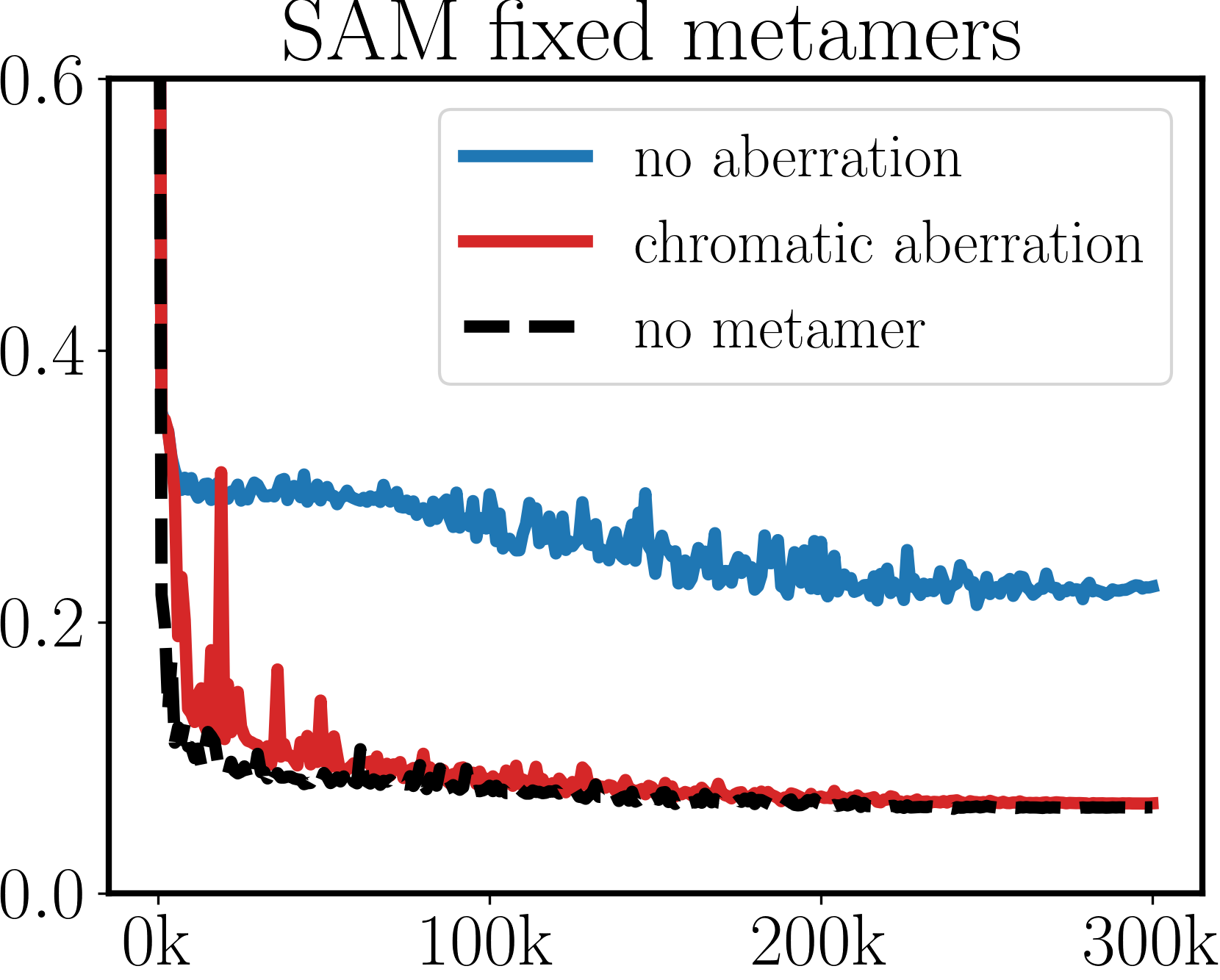
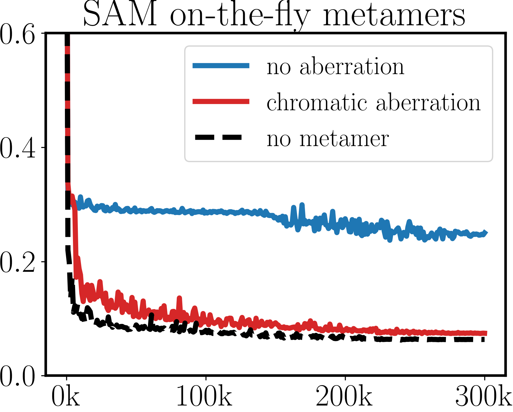
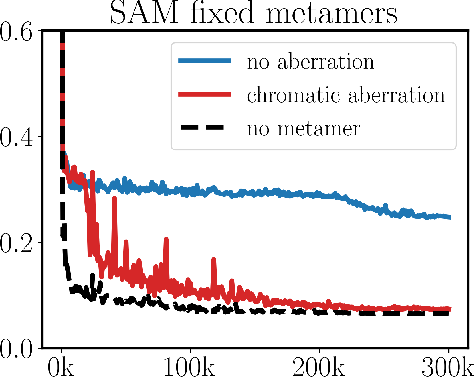
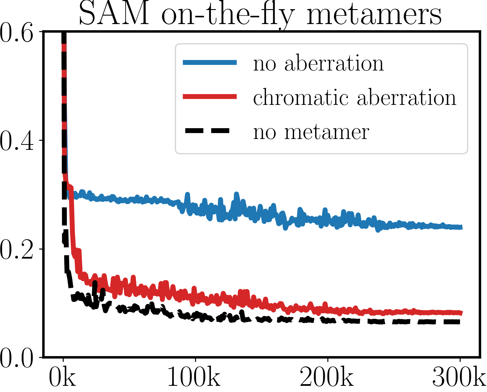
MPRNet		Restormer
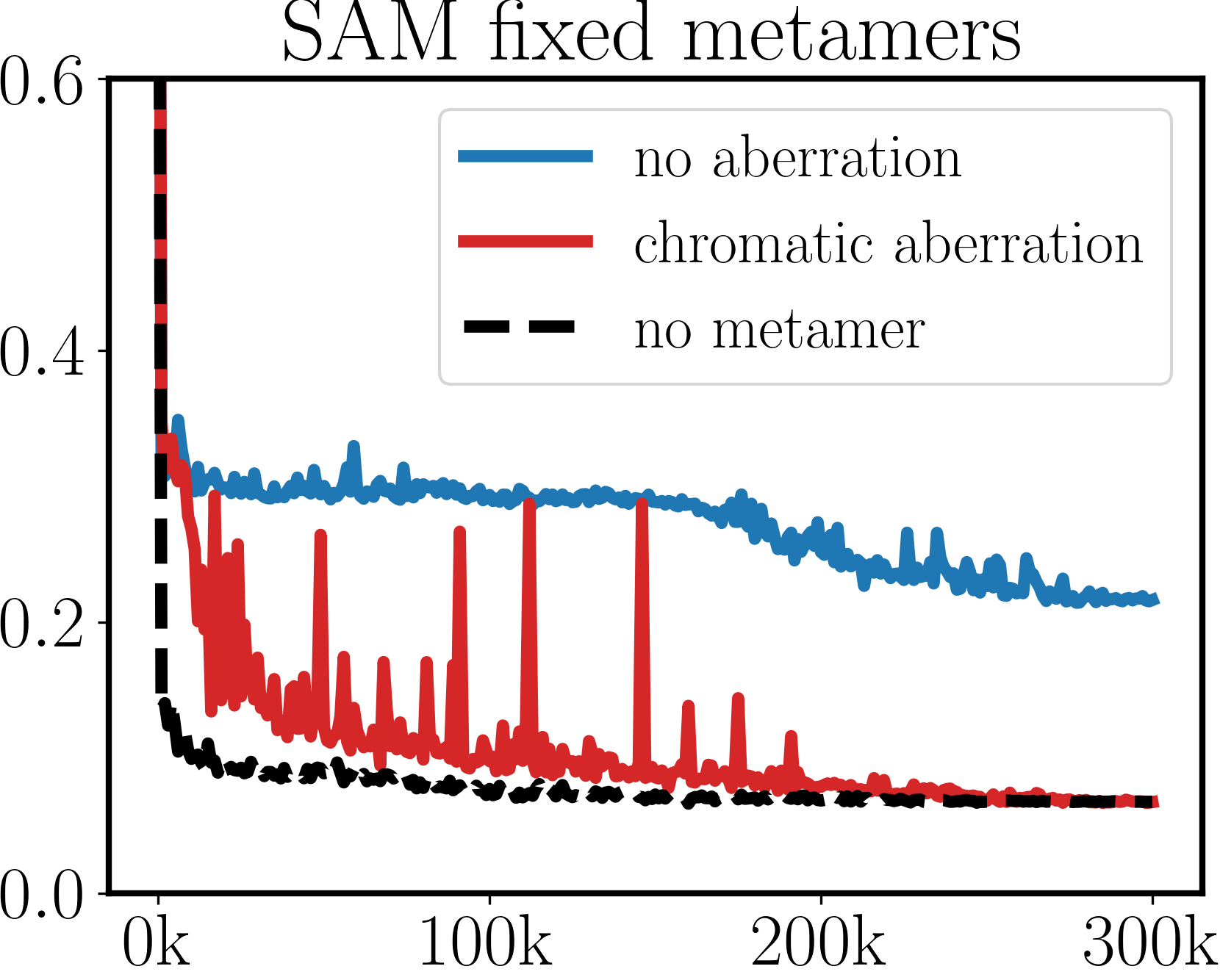
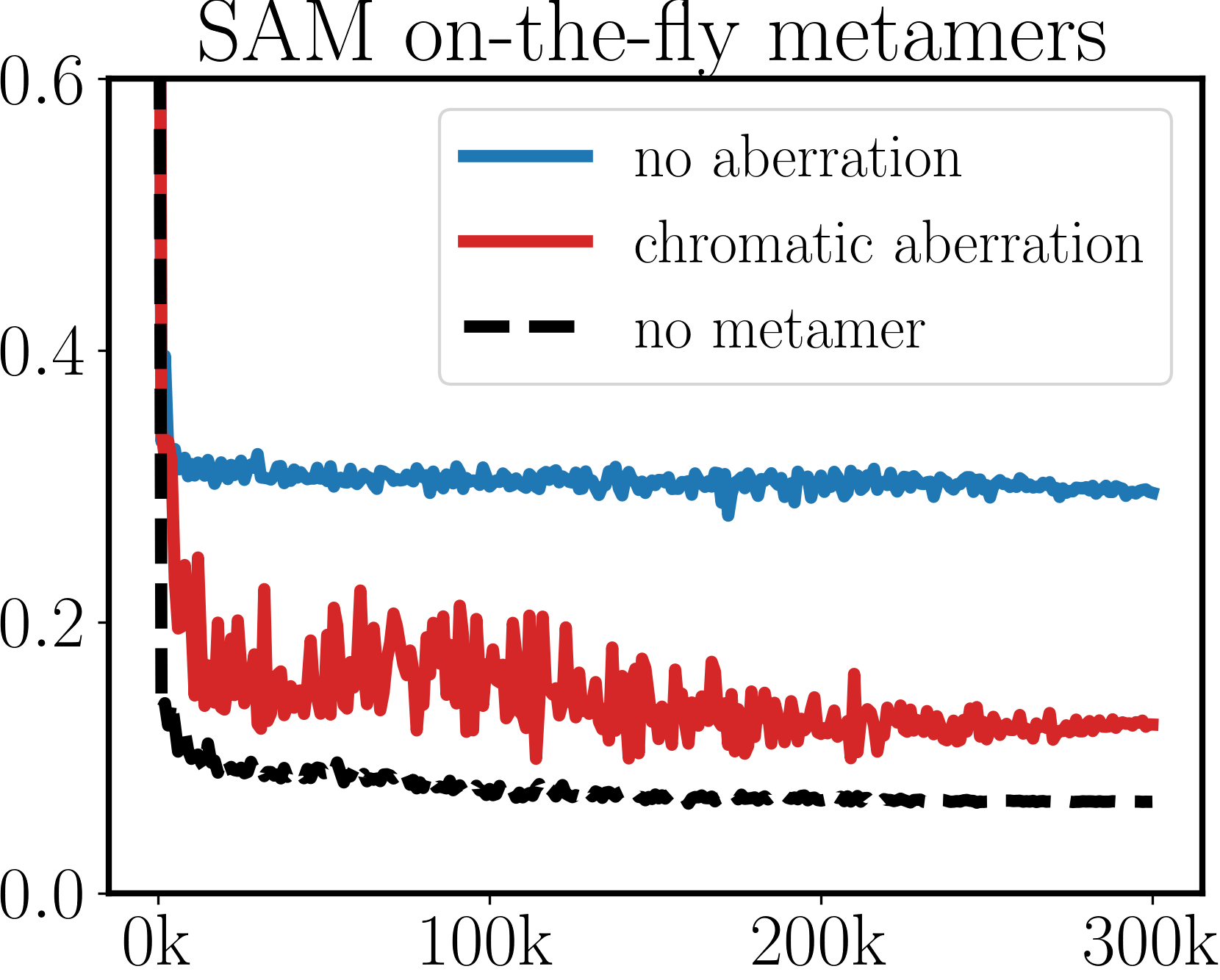
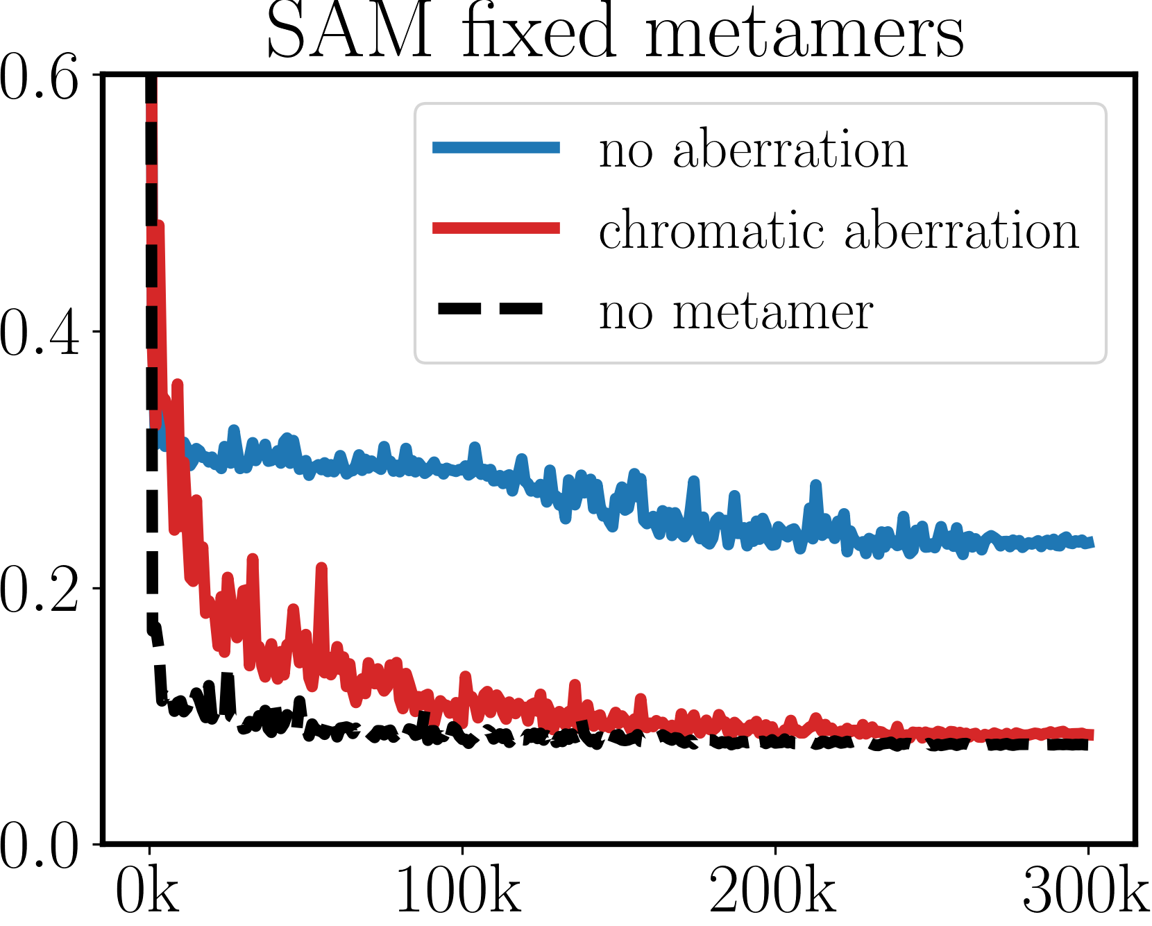
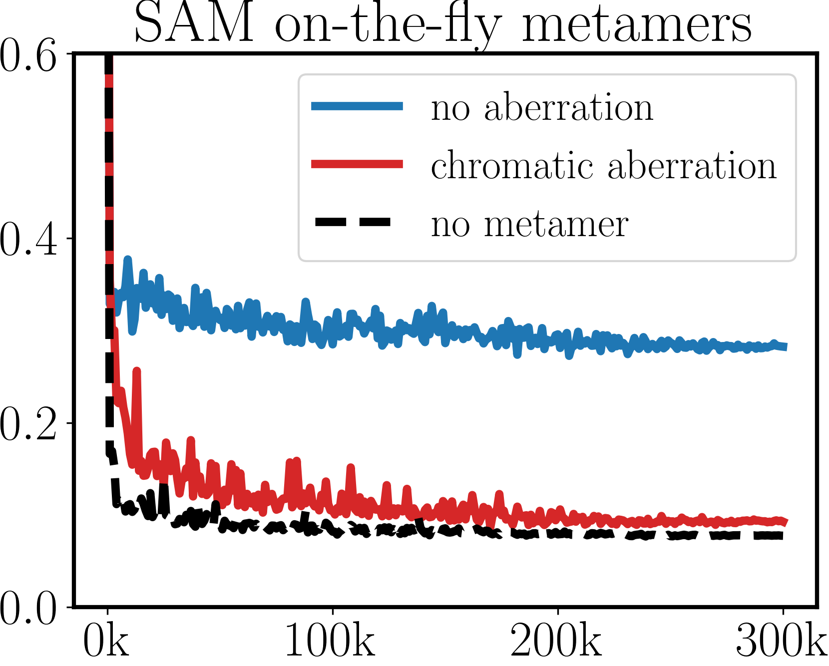
MIRNet		HINet

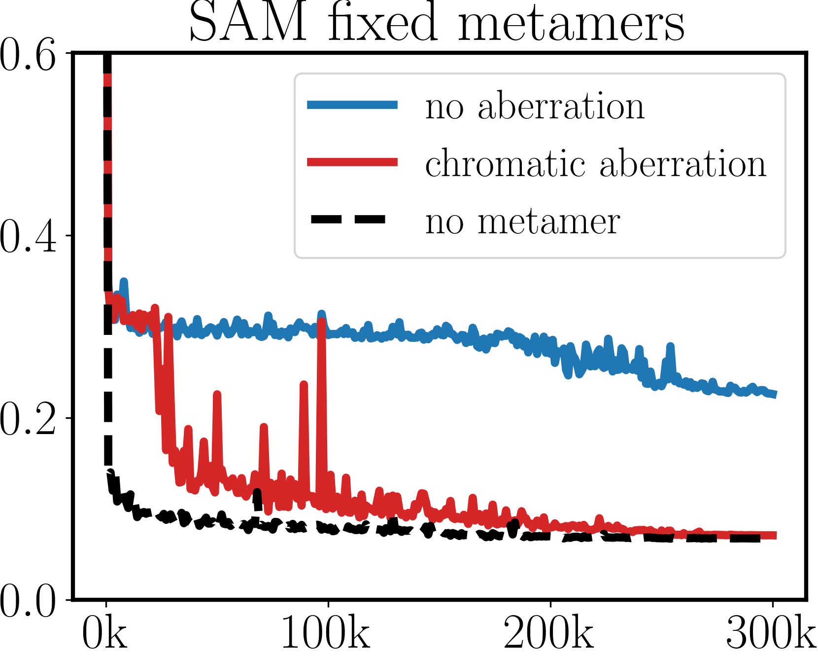
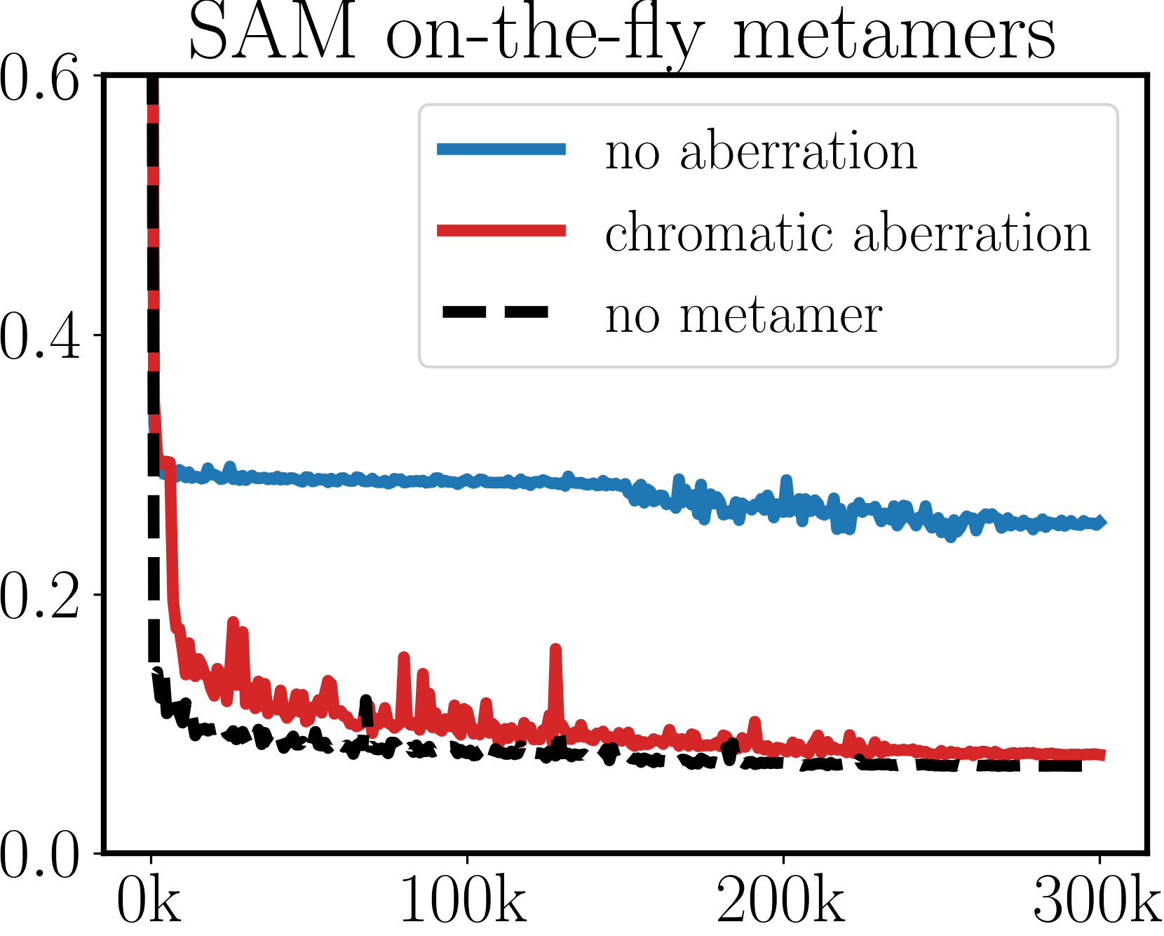
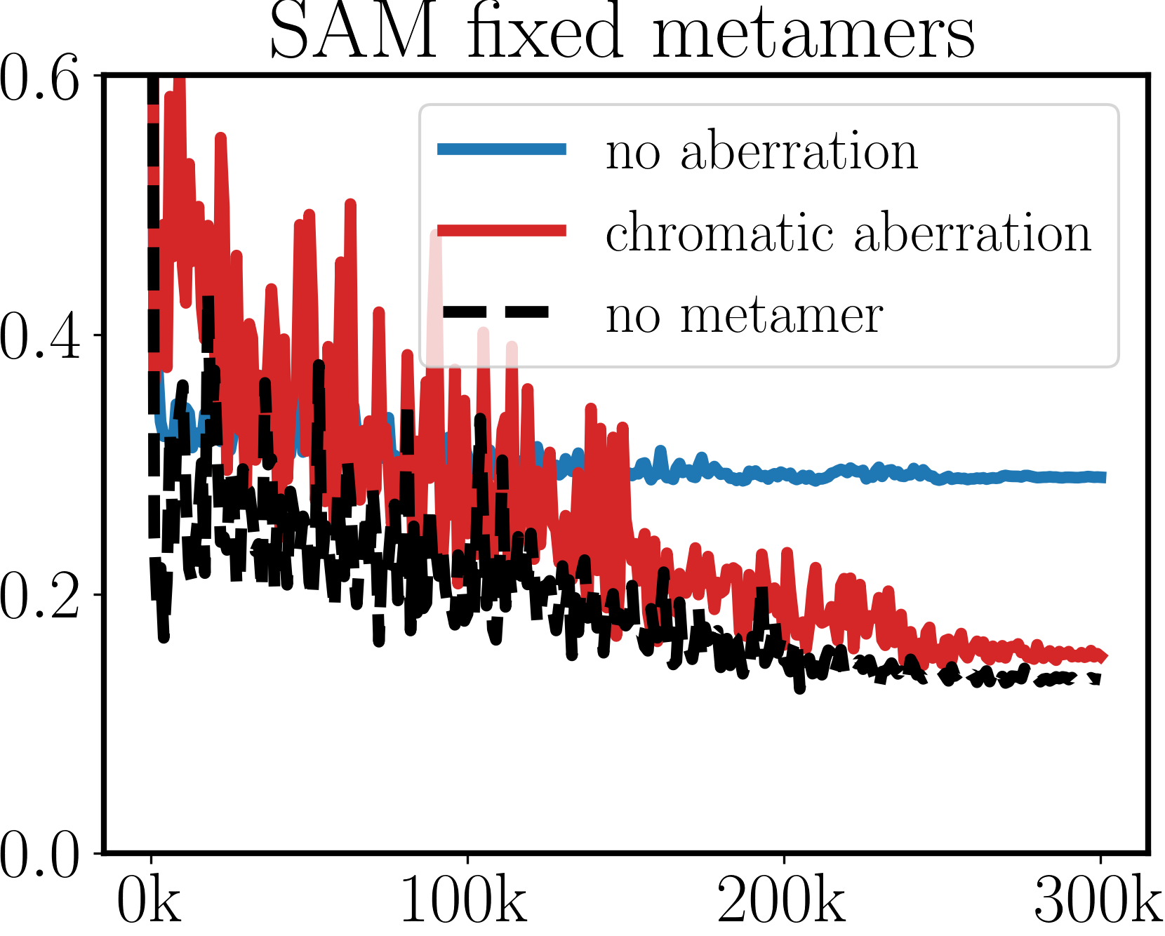
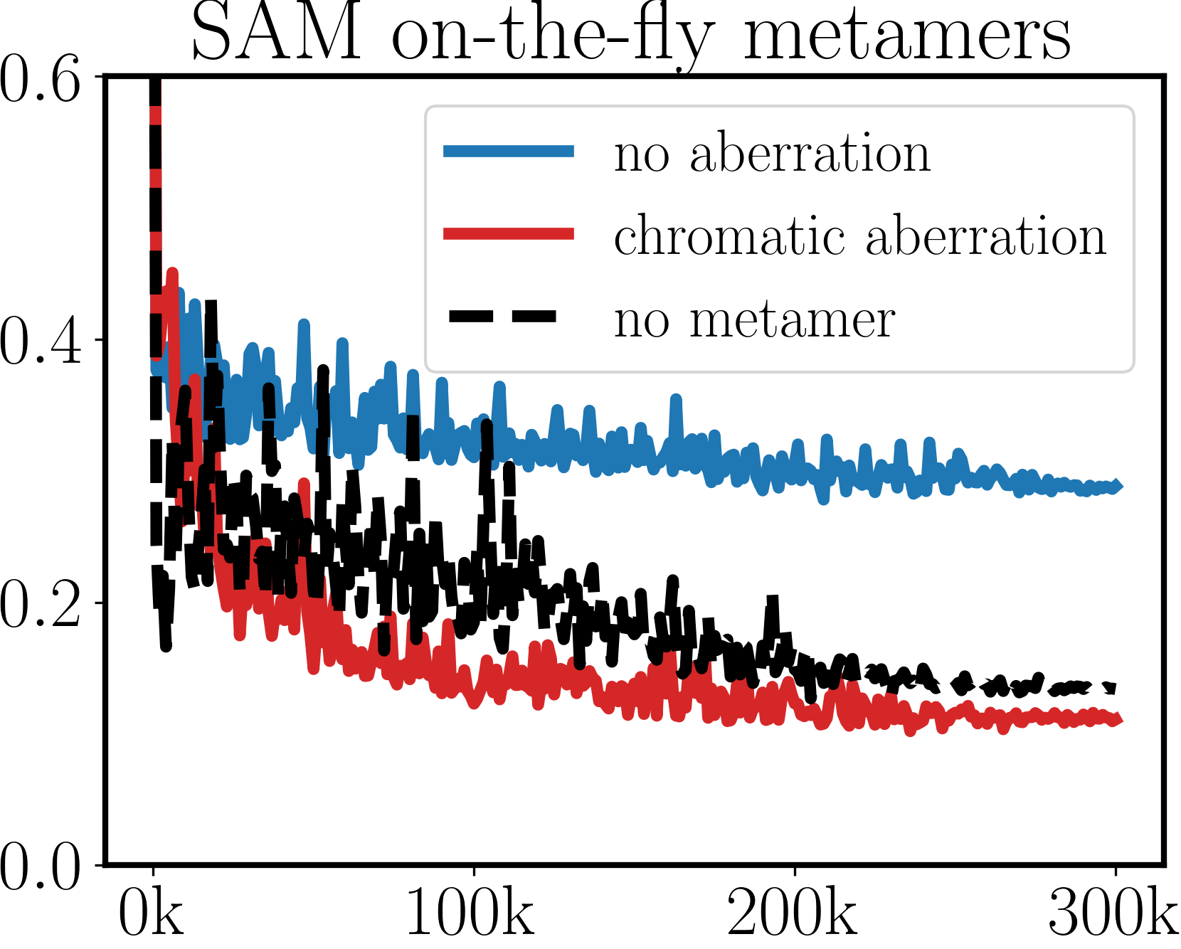
Figure 9: Chromatic aberrations improve spectral accuracy for MST++, MST-L, MPRNet, Restormer, MIRNet, and HINet. In each group, left: fixed metamers, and right: on-the-fly metamers.

HDNet		AWAN
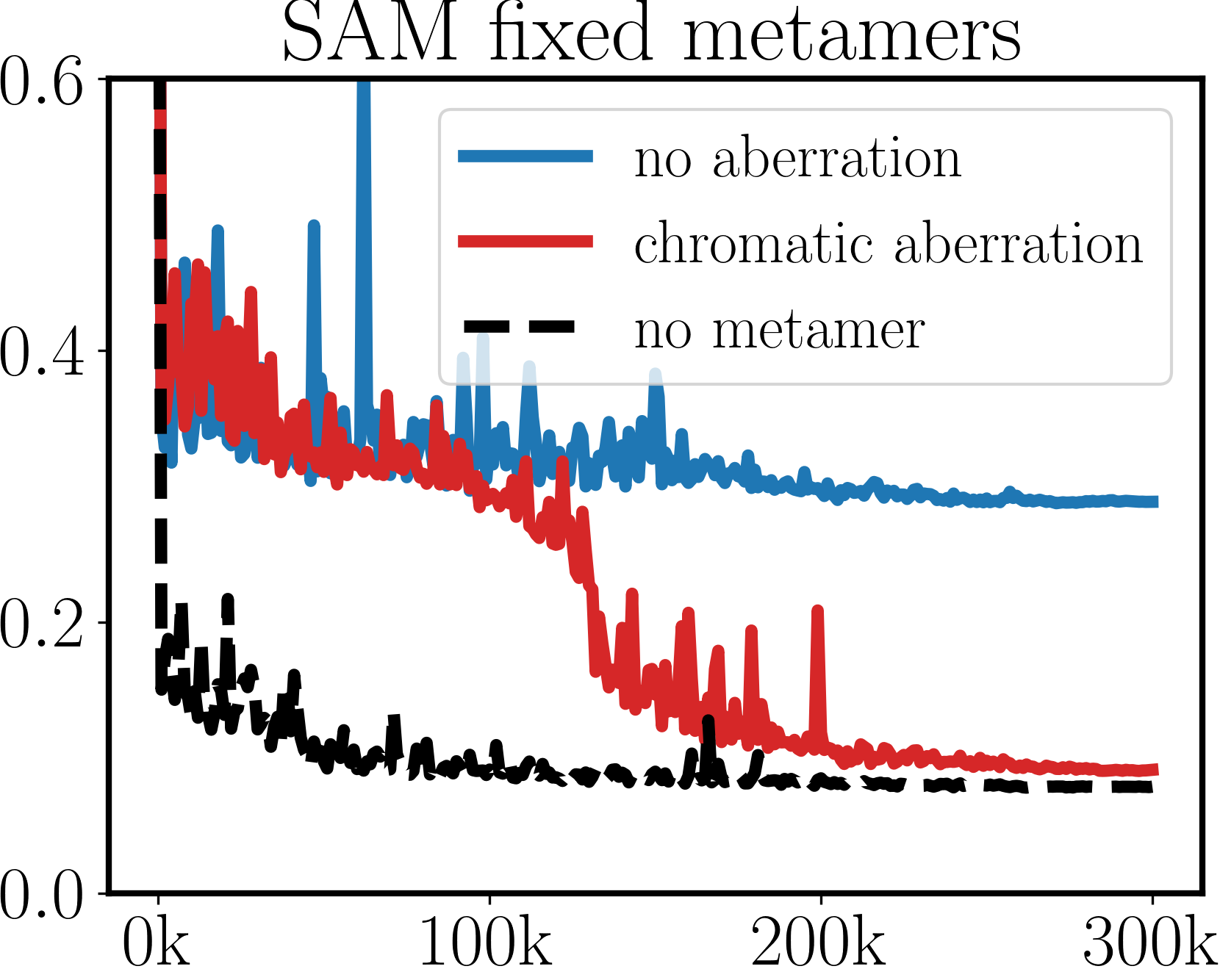
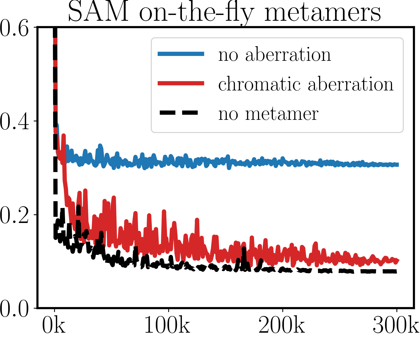
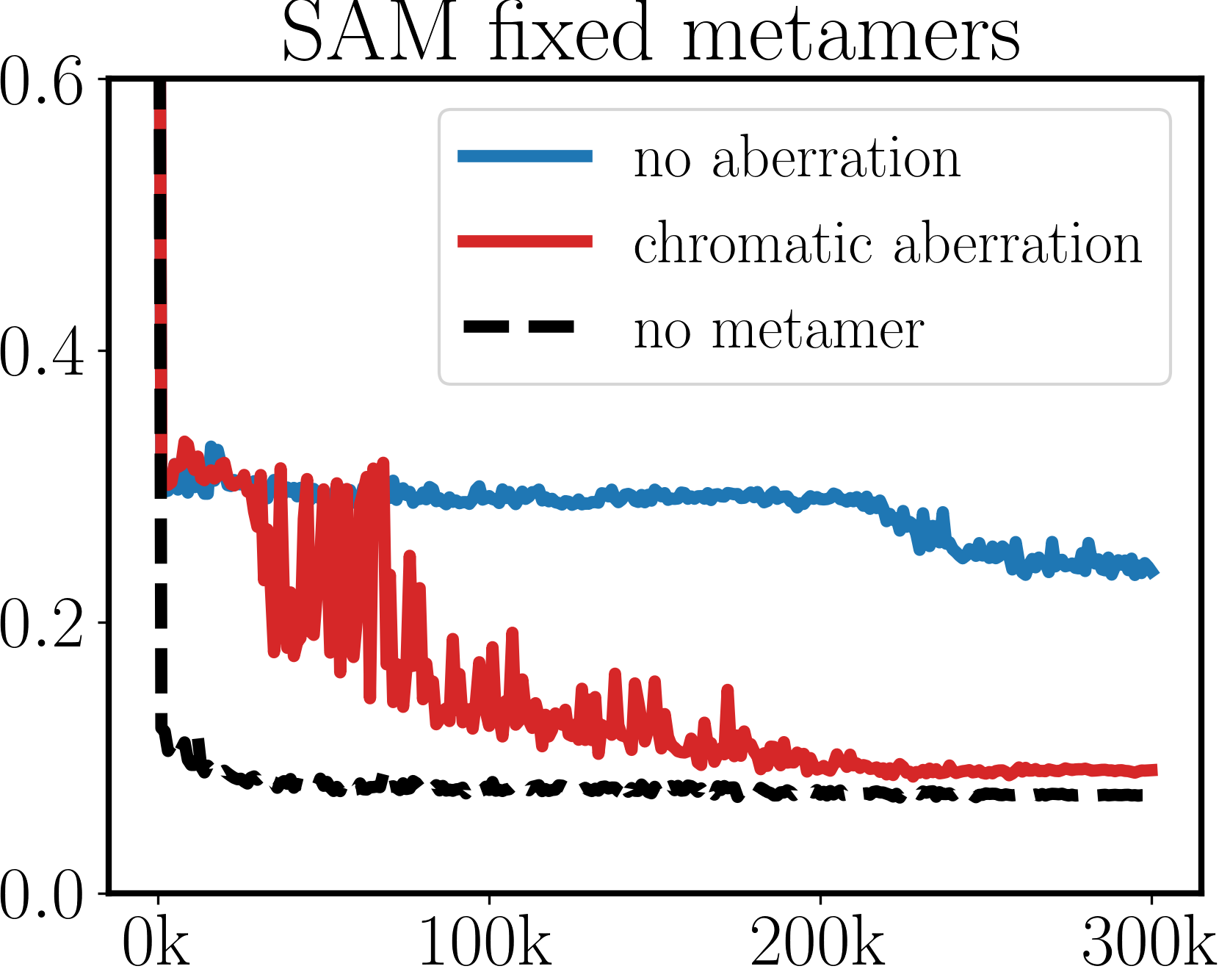
EDSR		HRNet
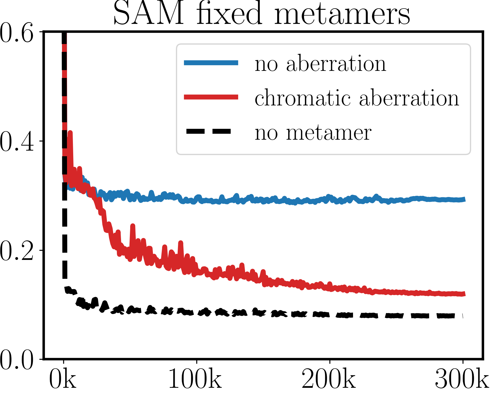
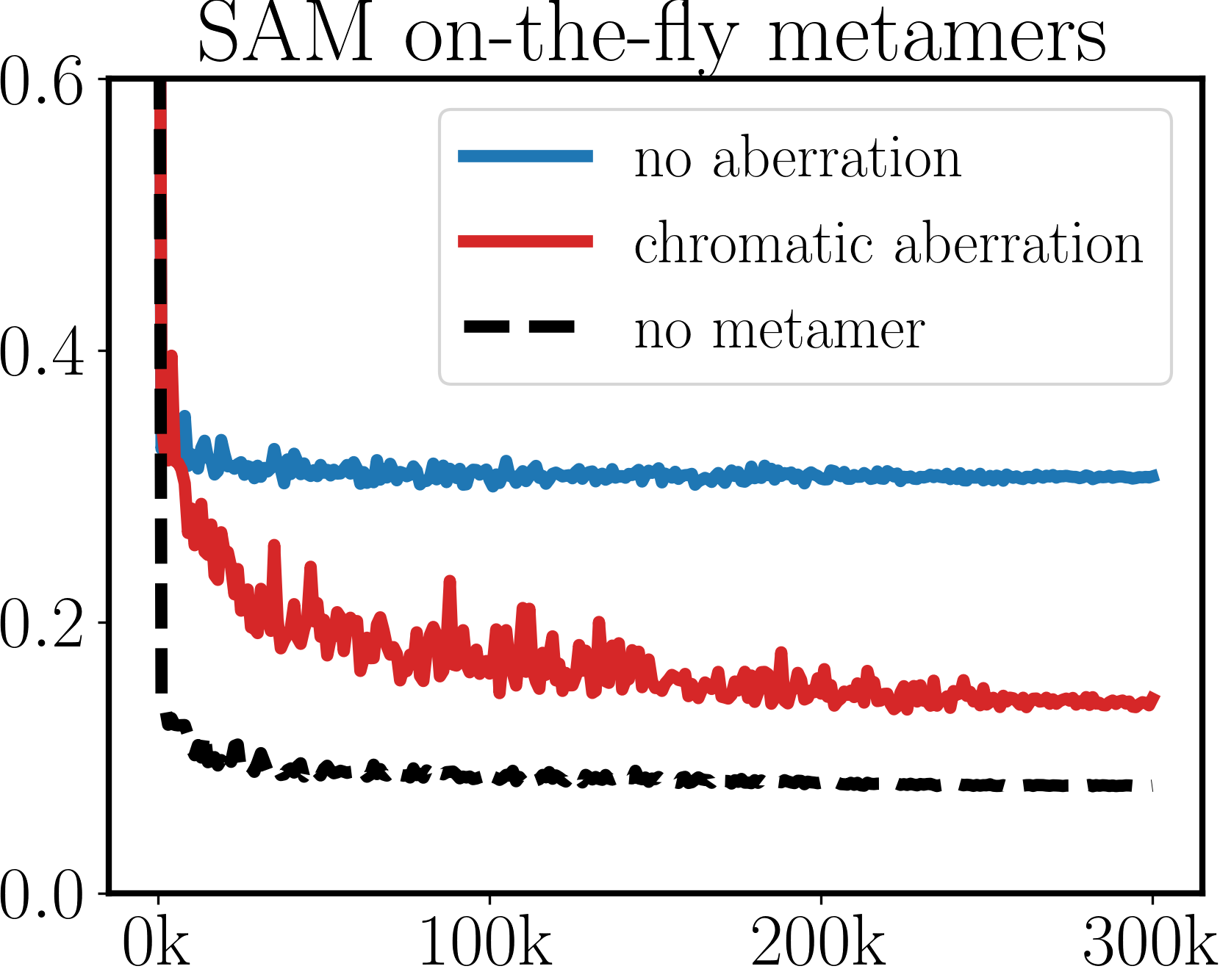
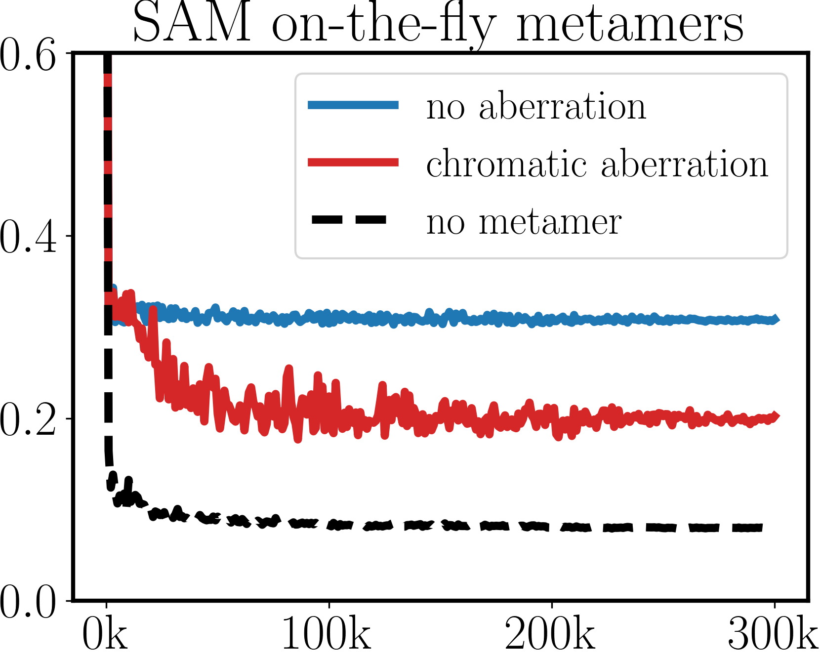
HSCNN+

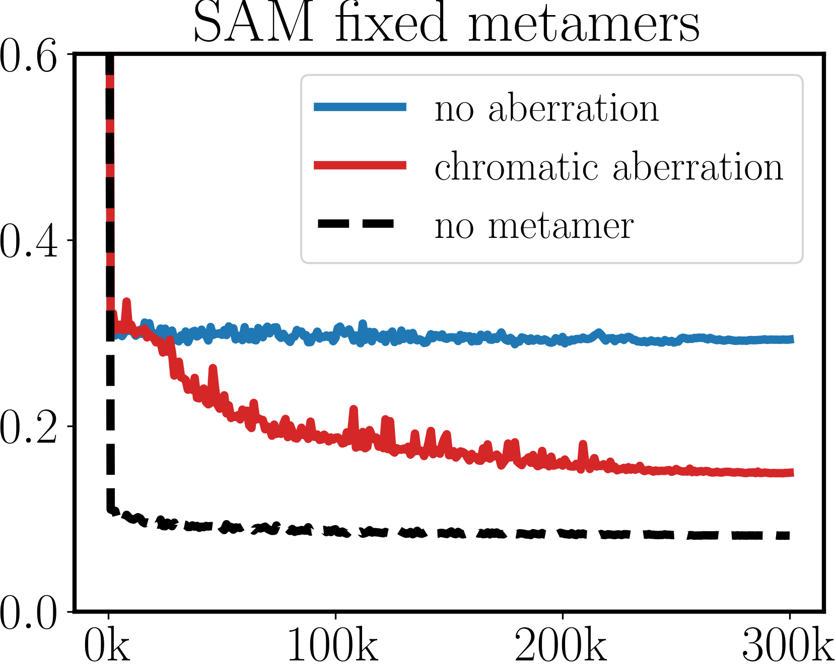
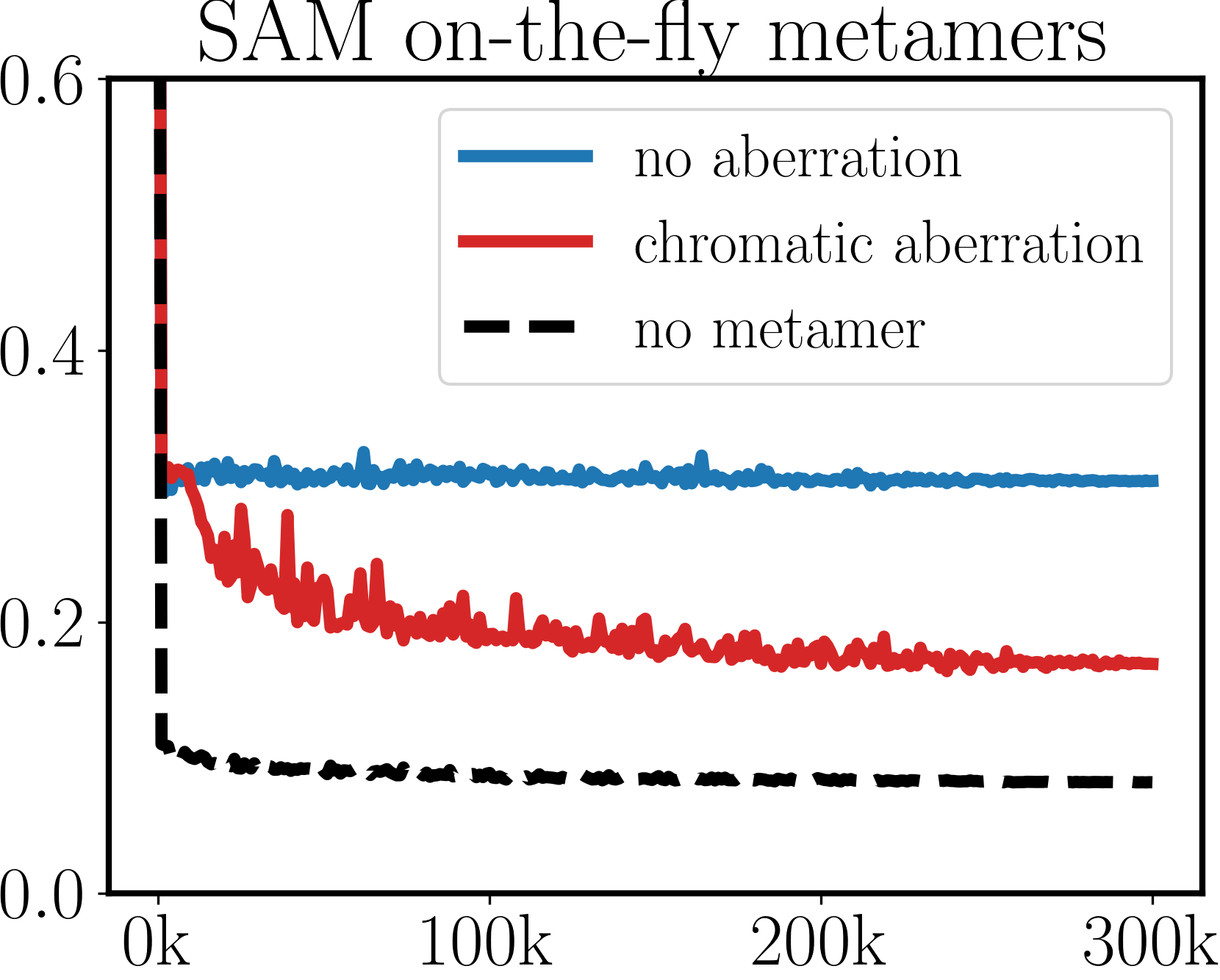
Figure 10: The aberration advantage results for HDNet, AWAN, EDSR, HRNet, and HSCNN+ on ARAD1K. In each group, left is for fixed metamers, and right is for on-the-fly metamers.

ARAD1K		CAVE
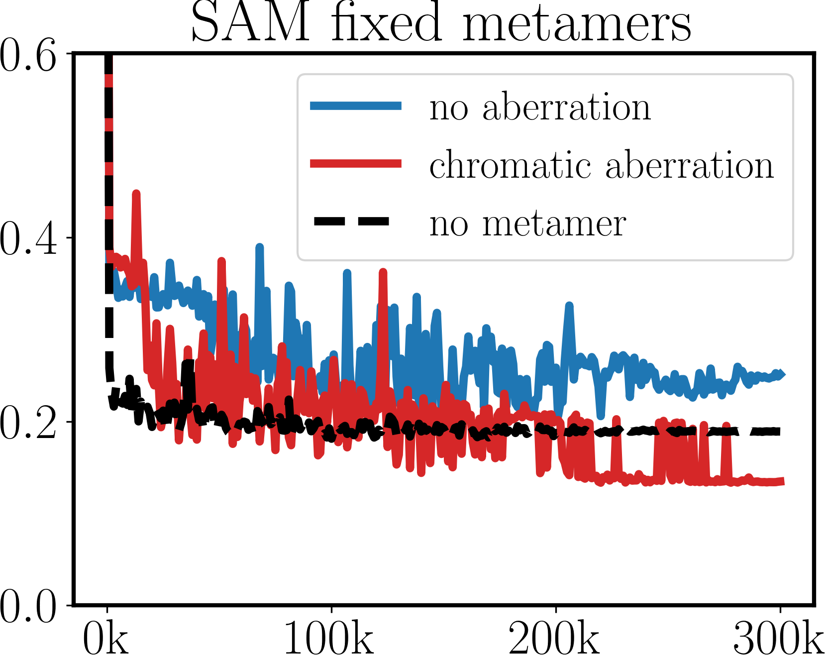
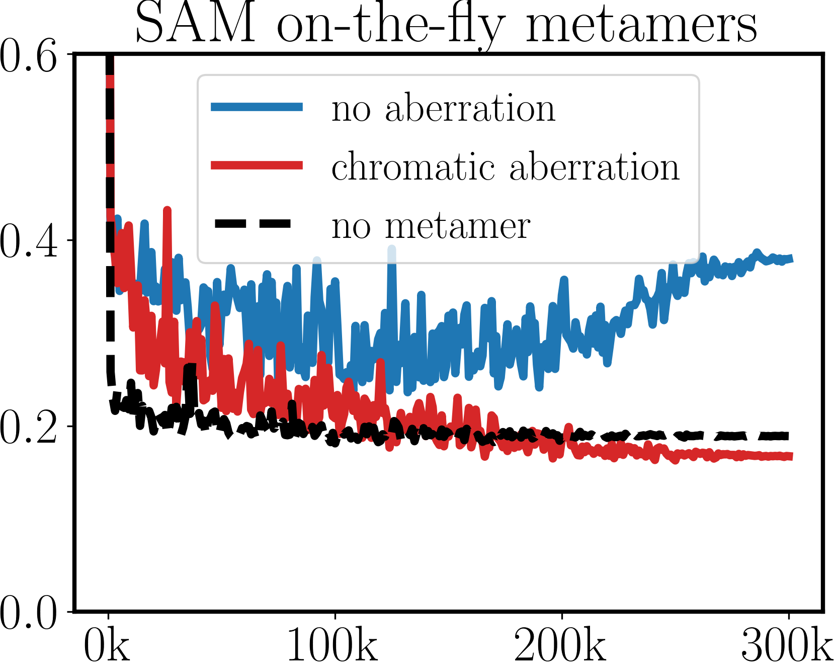
ICVL		KAUST

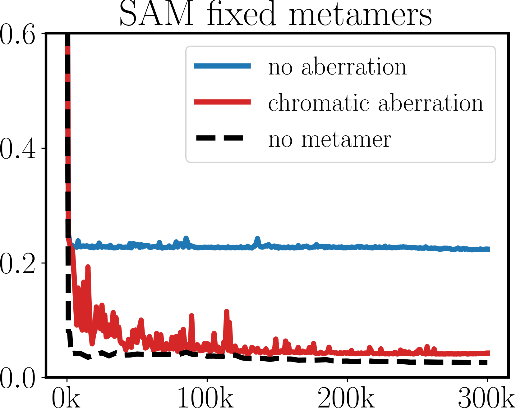
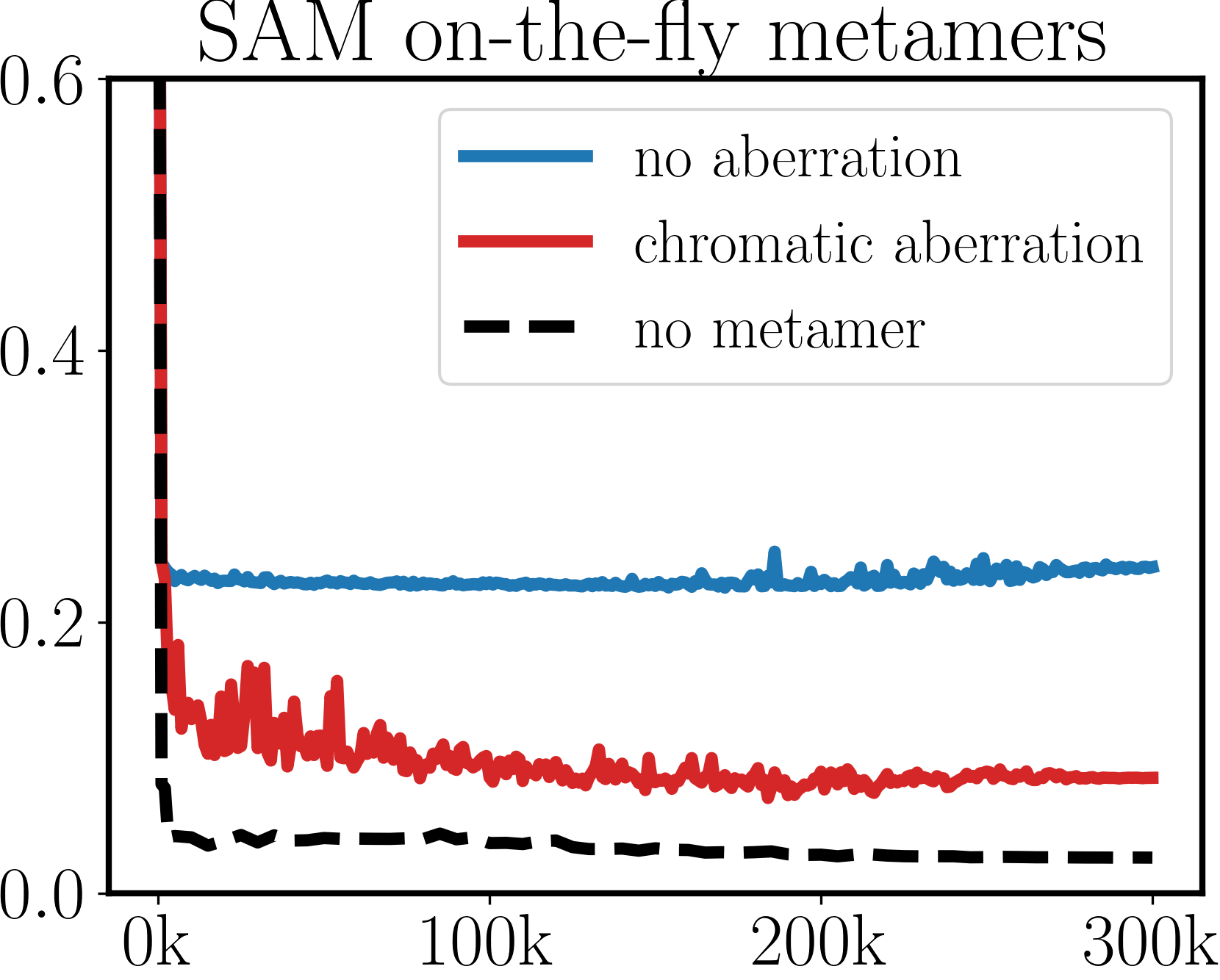
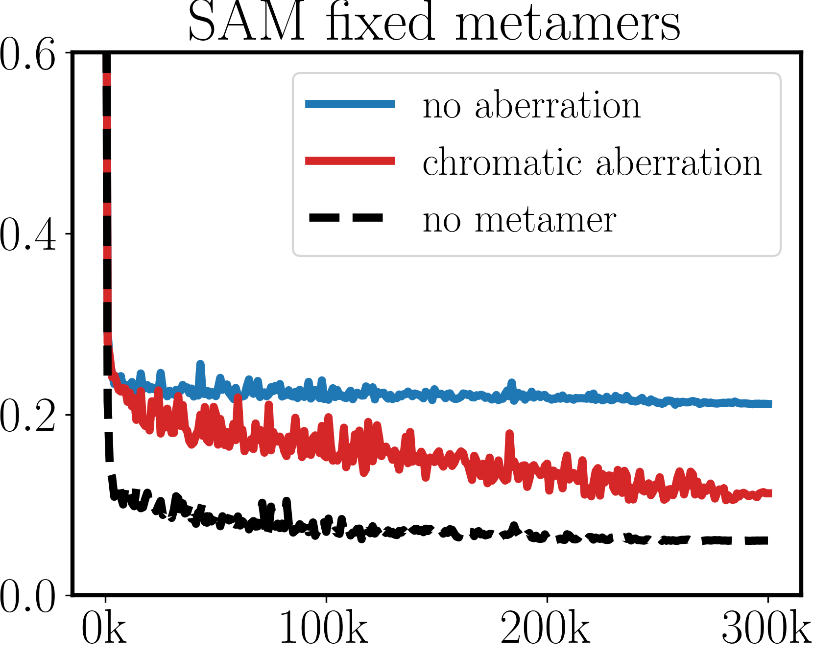
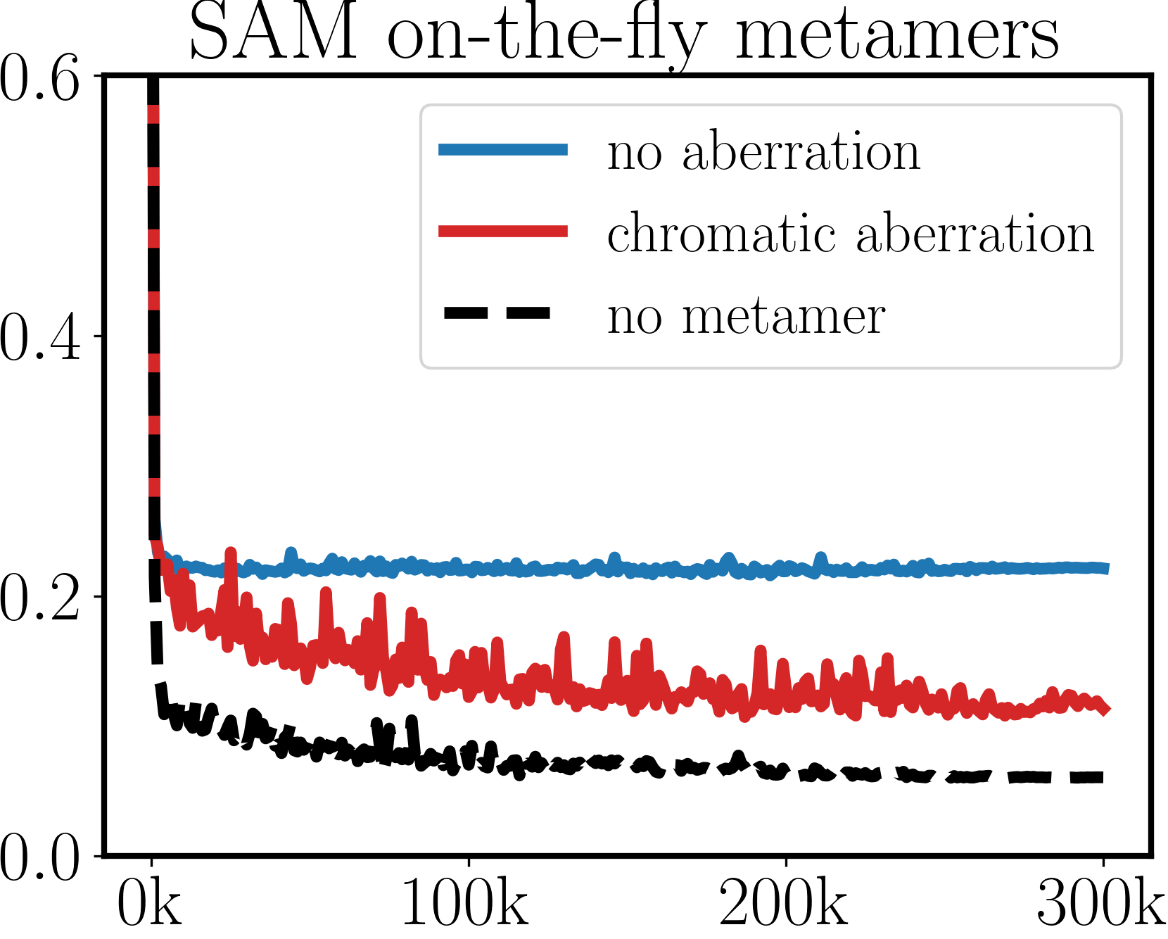
Figure 11: The aberration advantage results for MST++ on all datasets. In each group, left is for fixed metamers, and right is for on-the-fly metamers.

References

- Agustsson and Timofte [2017] Eirikur Agustsson and Radu Timofte. NTIRE 2017 challenge on single image super-resolution: Dataset and study. In IEEE Conf. Comput. Vis. Pattern Recog. Worksh., pages 126–135, 2017.
- Akbarinia and Gegenfurtner [2018] Arash Akbarinia and Karl R Gegenfurtner. Color metamerism and the structure of illuminant space. J. Opt. Soc. Am. A, 35(4):B231–B238, 2018.
- Alsam and Lenz [2007] Ali Alsam and Reiner Lenz. Calibrating color cameras using metameric blacks. J. Opt. Soc. Am. A, 24(1):11–17, 2007.
- Arad and Ben-Shahar [2016] Boaz Arad and Ohad Ben-Shahar. Sparse recovery of hyperspectral signal from natural RGB images. In Eur. Conf. Comput. Vis., pages 19–34. Springer, 2016.
- Arad et al. [2018] Boaz Arad, Ohad Ben-Shahar, Radu Timofte, L Van Gool, L Zhang, MH Yang, et al. NTIRE 2018 challenge on spectral reconstruction from RGB images. In IEEE Conf. Comput. Vis. Pattern Recog. Worksh., pages 1042–1042, 2018.
- Arad et al. [2020] Boaz Arad, Radu Timofte, Ohad Ben-Shahar, Yi-Tun Lin, and Graham D Finlayson. NTIRE 2020 challenge on spectral reconstruction from an RGB image. In IEEE Conf. Comput. Vis. Pattern Recog. Worksh., pages 446–447, 2020.
- Arad et al. [2022] Boaz Arad, Radu Timofte, Rony Yahel, Nimrod Morag, Amir Bernat, Yuanhao Cai, Jing Lin, Zudi Lin, Haoqian Wang, Yulun Zhang, et al. NTIRE 2022 spectral recovery challenge and data set. In IEEE Conf. Comput. Vis. Pattern Recog. Worksh., pages 863–881, 2022.
- Baek et al. [2017] Seung-Hwan Baek, Incheol Kim, Diego Gutierrez, and Min H Kim. Compact single-shot hyperspectral imaging using a prism. ACM Trans. Graph., 36(6):1–12, 2017.
- Banerjee et al. [2020] Bikram Pratap Banerjee, Simit Raval, and PJ Cullen. UAV-hyperspectral imaging of spectrally complex environments. Int. J. Remote Sens., 41(11):4136–4159, 2020.
- Bejani and Ghatee [2021] Mohammad Mahdi Bejani and Mehdi Ghatee. A systematic review on overfitting control in shallow and deep neural networks. Artif. Intell. Rev., pages 1–48, 2021.
- Belcour et al. [2023] L. Belcour, P. Barla, and G. Guennebaud. One-to-many spectral upsampling of reflectances and transmittances. Comput. Graph. Forum, 42(4):e14886, 2023.
- Cai et al. [2022a] Yuanhao Cai, Jing Lin, Xiaowan Hu, Haoqian Wang, Xin Yuan, Yulun Zhang, Radu Timofte, and Luc Van Gool. Mask-guided spectral-wise transformer for efficient hyperspectral image reconstruction. In IEEE Conf. Comput. Vis. Pattern Recog., pages 17502–17511, 2022a.
- Cai et al. [2022b] Yuanhao Cai, Jing Lin, Zudi Lin, Haoqian Wang, Yulun Zhang, Hanspeter Pfister, Radu Timofte, and Luc Van Gool. MST++: Multi-stage spectral-wise transformer for efficient spectral reconstruction. In IEEE Conf. Comput. Vis. Pattern Recog. Worksh., pages 745–755, 2022b.
- Cao et al. [2011] Xun Cao, Hao Du, Xin Tong, Qionghai Dai, and Stephen Lin. A prism-mask system for multispectral video acquisition. IEEE Trans. Pattern Anal. Mach. Intell., 33(12):2423–2435, 2011.
- Chakrabarti and Zickler [2011] Ayan Chakrabarti and Todd Zickler. Statistics of real-world hyperspectral images. In IEEE Conf. Comput. Vis. Pattern Recog., pages 193–200. IEEE, 2011.
- Chen et al. [2021] Liangyu Chen, Xin Lu, Jie Zhang, Xiaojie Chu, and Chengpeng Chen. HINet: Half instance normalization network for image restoration. In IEEE Conf. Comput. Vis. Pattern Recog., pages 182–192, 2021.
- Choi et al. [2017a] Inchang Choi, Daniel S. Jeon, Giljoo Nam, Diego Gutierrez, and Min H. Kim. High-quality hyperspectral reconstruction using a spectral prior. ACM Trans. Graph., 36(6):218:1–13, 2017a.
- Choi et al. [2017b] Inchang Choi, MH Kim, D Gutierrez, DS Jeon, and G Nam. High-quality hyperspectral reconstruction using a spectral prior. ACM Trans. Graph., 36(6):1–13, 2017b.
- Cohen and Kappauf [1982] Jozef B Cohen and William E Kappauf. Metameric color stimuli, fundamental metamers, and Wyszecki’s metameric blacks. Am. J. Psychol., pages 537–564, 1982.
- Cukierski and Foran [2010] William J Cukierski and David J Foran. Metamerism in multispectral imaging of histopathology specimens. In 2010 IEEE International Symposium on Biomedical Imaging: From Nano to Macro, pages 145–148. IEEE, 2010.
- Dale et al. [2013] Laura M Dale, André Thewis, Christelle Boudry, Ioan Rotar, Pierre Dardenne, Vincent Baeten, and Juan A Fernández Pierna. Hyperspectral imaging applications in agriculture and agro-food product quality and safety control: A review. Appl. Spectrosc. Rev., 48(2):142–159, 2013.
- Deng et al. [2009] Jia Deng, Wei Dong, Richard Socher, Li-Jia Li, Kai Li, and Li Fei-Fei. ImageNet: A large-scale hierarchical image database. In IEEE Conf. Comput. Vis. Pattern Recog., pages 248–255. Ieee, 2009.
- Fabbrizzi et al. [2022] Simone Fabbrizzi, Symeon Papadopoulos, Eirini Ntoutsi, and Ioannis Kompatsiaris. A survey on bias in visual datasets. Comput. Vis. Image Underst., 223:103552, 2022.
- Fauvel et al. [2012] Mathieu Fauvel, Yuliya Tarabalka, Jon Atli Benediktsson, Jocelyn Chanussot, and James C Tilton. Advances in spectral-spatial classification of hyperspectral images. Proc. IEEE, 101(3):652–675, 2012.
- Finlayson and Morovic [2005] Graham D Finlayson and Peter Morovic. Metamer sets. J. Opt. Soc. Am. A, 22(5):810–819, 2005.
- Foster and Amano [2019] David H Foster and Kinjiro Amano. Hyperspectral imaging in color vision research: tutorial. J. Opt. Soc. Am. A, 36(4):606–627, 2019.
- Foster et al. [2006] David H Foster, Kinjiro Amano, Sérgio MC Nascimento, and Michael J Foster. Frequency of metamerism in natural scenes. J. Opt. Soc. Am. A, 23(10):2359–2372, 2006.
- Hill [1999] Bernhard Hill. Color capture, color management, and the problem of metamerism: does multispectral imaging offer the solution? In Proc. SPIE, pages 2–14. SPIE, 1999.
- Hill [2002] Bernhard Hill. Optimization of total multispectral imaging systems: best spectral match versus least observer metamerism. In Proc. SPIE, pages 481–486. SPIE, 2002.
- Hu et al. [2022] Xiaowan Hu, Yuanhao Cai, Jing Lin, Haoqian Wang, Xin Yuan, Yulun Zhang, Radu Timofte, and Luc Van Gool. HDNet: High-resolution dual-domain learning for spectral compressive imaging. In IEEE Conf. Comput. Vis. Pattern Recog., pages 17542–17551, 2022.
- Huang et al. [2022] Longqian Huang, Ruichen Luo, Xu Liu, and Xiang Hao. Spectral imaging with deep learning. Light Sci. Appl., 11(1):61, 2022.
- Ichimura [2021] Junya Ichimura. Optical system and image pickup apparatus having the same, 2021. US Patent App. 17/174,832.
- Jakob and Hanika [2019] Wenzel Jakob and Johannes Hanika. A low-dimensional function space for efficient spectral upsampling. In Comput. Graph. Forum, pages 147–155. Wiley Online Library, 2019.
- Jeon et al. [2019] Daniel S Jeon, Seung-Hwan Baek, Shinyoung Yi, Qiang Fu, Xiong Dun, Wolfgang Heidrich, and Min H Kim. Compact snapshot hyperspectral imaging with diffracted rotation. ACM Trans. Graph., 38(4):1–13, 2019.
- Ji et al. [2023] Yuhyun Ji, Sang Mok Park, Semin Kwon, Jung Woo Leem, Vidhya Vijayakrishnan Nair, Yunjie Tong, and Young L Kim. mHealth hyperspectral learning for instantaneous spatiospectral imaging of hemodynamics. Proc. Natl. Acad. Sci., 2(4):pgad111, 2023.
- Kornblith et al. [2019] Simon Kornblith, Jonathon Shlens, and Quoc V Le. Do better ImageNet models transfer better? In IEEE Conf. Comput. Vis. Pattern Recog., pages 2661–2671, 2019.
- Kuching [2007] Sarawak Kuching. The performance of maximum likelihood, spectral angle mapper, neural network and decision tree classifiers in hyperspectral image analysis. J. Comput. Sci., 3(6):419–423, 2007.
- Li et al. [2020] Jiaojiao Li, Chaoxiong Wu, Rui Song, Yunsong Li, and Fei Liu. Adaptive weighted attention network with camera spectral sensitivity prior for spectral reconstruction from RGB images. In IEEE Conf. Comput. Vis. Pattern Recog. Worksh., pages 462–463, 2020.
- Li et al. [2021] Yuqi Li, Qiang Fu, and Wolfgang Heidrich. Multispectral illumination estimation using deep unrolling network. In Int. Conf. Comput. Vis., pages 2672–2681, 2021.
- Lim et al. [2017] Bee Lim, Sanghyun Son, Heewon Kim, Seungjun Nah, and Kyoung Mu Lee. Enhanced deep residual networks for single image super-resolution. In IEEE Conf. Comput. Vis. Pattern Recog. Worksh., pages 136–144, 2017.
- Lodhi et al. [2019] Vaibhav Lodhi, Debashish Chakravarty, and Pabitra Mitra. Hyperspectral imaging system: Development aspects and recent trends. Sens. Imaging, 20:1–24, 2019.
- Lu and Fei [2014] Guolan Lu and Baowei Fei. Medical hyperspectral imaging: a review. J. Biomed. Opt., 19(1):010901–010901, 2014.
- Monno et al. [2015] Yusukex Monno, Sunao Kikuchi, Masayuki Tanaka, and Masatoshi Okutomi. A practical one-shot multispectral imaging system using a single image sensor. IEEE Trans. Image Process., 24(10):3048–3059, 2015.
- Ortega et al. [2020] Samuel Ortega, Martin Halicek, Himar Fabelo, Gustavo M Callico, and Baowei Fei. Hyperspectral and multispectral imaging in digital and computational pathology: a systematic review. Biomed. Opt. Express, 11(6):3195–3233, 2020.
- Park et al. [2007] Bosoon Park, WR Windham, KC Lawrence, and DP Smith. Contaminant classification of poultry hyperspectral imagery using a spectral angle mapper algorithm. Biosyst. Eng., 96(3):323–333, 2007.
- Prasad and Wenhe [2015] Dilip K Prasad and Looi Wenhe. Metrics and statistics of frequency of occurrence of metamerism in consumer cameras for natural scenes. J. Opt. Soc. Am. A, 32(7):1390–1402, 2015.
- Rangnekar et al. [2022] Aneesh Rangnekar, Zachary Mulhollan, Anthony Vodacek, Matthew Hoffman, Angel D Sappa, Erik Blasch, Jun Yu, Liwen Zhang, Shenshen Du, Hao Chang, et al. Semi-supervised hyperspectral object detection challenge results-pbvs 2022. In IEEE Conf. Comput. Vis. Pattern Recog., pages 390–398, 2022.
- Rebuffi et al. [2021] Sylvestre-Alvise Rebuffi, Sven Gowal, Dan Andrei Calian, Florian Stimberg, Olivia Wiles, and Timothy A Mann. Data augmentation can improve robustness. Adv. Neural Inf. Process., 34:29935–29948, 2021.
- Saragadam and Sankaranarayanan [2019] Vishwanath Saragadam and Aswin C Sankaranarayanan. KRISM—Krylov subspace-based optical computing of hyperspectral images. ACM Trans. Graph., 38(5):1–14, 2019.
- Shi et al. [2018] Zhan Shi, Chang Chen, Zhiwei Xiong, Dong Liu, and Feng Wu. HSCNN+: Advanced CNN-based hyperspectral recovery from RGB images. In IEEE Conf. Comput. Vis. Pattern Recog. Worksh., pages 939–947, 2018.
- Shorten and Khoshgoftaar [2019] Connor Shorten and Taghi M Khoshgoftaar. A survey on image data augmentation for deep learning. J. Big Data, 6(1):1–48, 2019.
- Thornton [1998] William A Thornton. How strong metamerism disturbs color spaces. Color Res. Appl., 23(6):402–407, 1998.
- Torralba and Efros [2011] Antonio Torralba and Alexei A Efros. Unbiased look at dataset bias. In IEEE Conf. Comput. Vis. Pattern Recog., pages 1521–1528. IEEE, 2011.
- Van De Ruit and Eisemann [2023] Mark Van De Ruit and Elmar Eisemann. Metameric: Spectral uplifting via controllable color constraints. In ACM SIGGRAPH 2023 Conference Proceedings, pages 1–10, 2023.
- Van der Meer [2006] Freek Van der Meer. The effectiveness of spectral similarity measures for the analysis of hyperspectral imagery. Int. J. Appl. Earth Obs. Geoinf., 8(1):3–17, 2006.
- van Trigt [1994] Cornelius van Trigt. Metameric blacks and estimating reflectance. J. Opt. Soc. Am. A, 11(3):1003–1024, 1994.
- Viénot and Brettel [2014] Françoise Viénot and Hans Brettel. The verriest lecture: Visual properties of metameric blacks beyond cone vision. J. Opt. Soc. Am. A, 31(4):A38–A46, 2014.
- Wagadarikar et al. [2008] Ashwin Wagadarikar, Renu John, Rebecca Willett, and David Brady. Single disperser design for coded aperture snapshot spectral imaging. Appl. Opt., 47(10):B44–B51, 2008.
- Weidlich et al. [2021] Andrea Weidlich, Alex Forsythe, Scott Dyer, Thomas Mansencal, Johannes Hanika, Alexander Wilkie, Luke Emrose, and Anders Langlands. Spectral imaging in production: course notes SIGGRAPH 2021. In ACM SIGGRAPH 2021 Courses, pages 1–90. Association for Computing Machinery (ACM), 2021.
- Werpachowski et al. [2019] Roman Werpachowski, András György, and Csaba Szepesvári. Detecting overfitting via adversarial examples. Adv. Neural Inf. Process., 32, 2019.
- Yang et al. [2023] Xinge Yang, Qiang Fu, Mohamed Elhoseiny, and Wolfgang Heidrich. Aberration-aware depth-from-focus. IEEE Trans. Pattern Anal. Mach. Intell., 2023.
- Yasuma et al. [2010] Fumihito Yasuma, Tomoo Mitsunaga, Daisuke Iso, and Shree K Nayar. Generalized assorted pixel camera: postcapture control of resolution, dynamic range, and spectrum. IEEE Trans. Image Process., 19(9):2241–2253, 2010.
- Zamir et al. [2020] Syed Waqas Zamir, Aditya Arora, Salman Khan, Munawar Hayat, Fahad Shahbaz Khan, Ming-Hsuan Yang, and Ling Shao. Learning enriched features for real image restoration and enhancement. In Eur. Conf. Comput. Vis., pages 492–511. Springer, 2020.
- Zamir et al. [2021] Syed Waqas Zamir, Aditya Arora, Salman Khan, Munawar Hayat, Fahad Shahbaz Khan, Ming-Hsuan Yang, and Ling Shao. Multi-stage progressive image restoration. In IEEE Conf. Comput. Vis. Pattern Recog., pages 14821–14831, 2021.
- Zamir et al. [2022] Syed Waqas Zamir, Aditya Arora, Salman Khan, Munawar Hayat, Fahad Shahbaz Khan, and Ming-Hsuan Yang. Restormer: Efficient transformer for high-resolution image restoration. In IEEE Conf. Comput. Vis. Pattern Recog., pages 5728–5739, 2022.
- Zhang et al. [2022] Jingang Zhang, Runmu Su, Qiang Fu, Wenqi Ren, Felix Heide, and Yunfeng Nie. A survey on computational spectral reconstruction methods from RGB to hyperspectral imaging. Sci. Rep., 12(1):11905, 2022.
- Zhao et al. [2020] Yuzhi Zhao, Lai-Man Po, Qiong Yan, Wei Liu, and Tingyu Lin. Hierarchical regression network for spectral reconstruction from RGB images. In IEEE Conf. Comput. Vis. Pattern Recog. Worksh., pages 422–423, 2020.