Simultaneous false discovery bounds for invariant causal prediction

Abstract

Invariant causal prediction (ICP, Peters et al., (2016)) provides a novel way to identify causal predictors of a response by utilizing heterogeneous data from different environments. One advantage of ICP is that it guarantees to make no false causal discoveries with high probability. Such a guarantee, however, can be too conservative in some applications, resulting in few or no discoveries. To address this, we propose simultaneous false discovery bounds for ICP, which provides users with extra flexibility in exploring causal predictors and can extract more informative results. These additional inferences come for free, in the sense that they do not require additional assumptions, and the same information obtained by the original ICP is retained. We demonstrate the practical usage of our method through simulations and a real dataset.

1 Introduction

Discovering causal predictors of the response of interest is usually the primary goal of scientific research. Based solely on observational data, the causal relationship might be unidentifiable. In such cases, heterogeneous data from different environments can be helpful for further identifiability and thus is a valuable source for causal discovery. Under the multi-environments setting, Peters et al., (2016) proposed a novel method, called invariant causal prediction (ICP), to identify causal predictors of a response by exploiting the invariance of the conditional distribution of the response given its causal predictors across environments. Compared to other causal discovery algorithms, one main advantage of ICP is that it provides a statistical confidence guarantee for its output $\widehat{S}^{\text{ICP}}$:

$$P\left(\widehat{S}^{\text{ICP}}\subseteq S^{*}\right)\geq 1-\alpha,$$

where $\alpha\in(0,1)$ is a nominal level and $S^{*}$ denotes the set of true causal predictors. That is, ICP ensures that all its discoveries are true causal predictors with a probability larger than $1-\alpha$. This is also known as the familywise error rate control guarantee.

The original ICP approach has been generalized to non-linear setting (Heinze-Deml et al.,, 2018), sequential data (Pfister et al.,, 2019), and transformation models (Kook et al.,, 2023). All these methods inherit the familywise error rate control guarantee. However, controlling the familywise error rate can be too conservative in many applications, especially when causal predictors are highly correlated with non-causal ones. In such cases, ICP may result in few or no causal discoveries. To address this, Heinze-Deml et al., (2018) proposed the so-called defining sets, which are the smallest sets guaranteeing to contain at least one true causal predictor. They are especially useful in the case where ICP returns an empty set.

In this paper, we propose a method to obtain simultaneous false discovery bound (Genovese and Wasserman,, 2006; Goeman and Solari,, 2011; Goeman et al.,, 2021) for ICP. Specifically, let $\mathcal{N}^{*}\subseteq[m]=\{1,\dots,m\}$ be the index set of non-causal predictors among $m$ predictors, the simultaneous false discovery bound is a function $t_{\alpha}:2^{[m]}\rightarrow\{0,\dots,m\}$, where $2^{m}$ denotes the power set of $[m]$, such that

$$P(|R\cap\mathcal{N}^{*}|\leq t_{\alpha}(R)\text{ for any }R\subseteq[m])\geq 1-\alpha.$$

As a result, one can freely check any set $R$ of interest, and a high probability upper bound of the false discoveries can be obtained by $t_{\alpha}(R)$. This contains the familywise error rate control and the defining sets of Heinze-Deml et al., (2018) as special cases. In particular, by searching for the largest set $R$ whose corresponding $t_{\alpha}(R)$ is $0$, we obtain a set with familywise error rate control; by searching for the smallest sets whose corresponding $t_{\alpha}(R)\leq|R|-1$, we obtain all defining sets.

Extra causal information can be extracted using the simultaneous false discovery bound. As a quick illustration, for a simulated dataset with nine predictors shown in Section 4.1, no information is obtained by the original ICP approach as it returns zero discoveries. However, more causal information can be extracted by using our simultaneous false discovery bounds. For example, we can know that with a probability larger than $0.95$, there is at least one causal predictor in $\{X_{3},X_{7}\}$, at least two causal predictors in $\{X_{3},X_{5},X_{7},X_{8}\}$, and at least four causal predictors in all nine predictors. More simulations and a real data application can be found in Section 4.1.

To obtain the simultaneous false discovery bound for ICP, we proceed by considering a multiple testing problem (see (6)) that directly tests causal predictors. We show that the original ICP approach is equivalent to directly comparing certain p-values (see (8)) to the significance level. Then, by generalizing the null hypothesis (6) and p-value (7) to (10) and (11), respectively, we propose a simultaneous false discovery upper bound (12). This upper bound can be seen as a special case of the closed testing method by Goeman and Solari, (2011), but in our case, no closed testing adjustment is needed due to the specific form of the p-values. In comparison to the original ICP approach, our method provides additional causal information at the cost of testing more hypotheses, without introducing any additional statistical assumptions. We also discuss the idea of controlling the false discovery rate for ICP.

2 A brief recap of invariant causal prediction

For the sake of simplicity, we use linear models (Peters et al.,, 2016) for illustration. Consider the following linear structural equation model:

$$Y^{e}\leftarrow\beta_{1}X^{e}_{1}+\cdots\beta_{m}X^{e}_{m}+\epsilon^{e}=\beta_{S^{*}}^{T}X^{e}_{S^{*}}+\epsilon^{e},$$ (1)

where $S^{*}=\{i\in[m]:\beta_{i}\neq 0\}$ is the set of causal predictors of $Y$, $e\in\mathcal{E}$ denotes one environment, $\epsilon^{e}\sim F_{\epsilon}$, $\epsilon^{e}\mathchoice{\mathrel{\hbox to0.0pt{$\displaystyle\perp$\hss}\mkern 2.0mu{\displaystyle\perp}}}{\mathrel{\hbox to0.0pt{$\textstyle\perp$\hss}\mkern 2.0mu{\textstyle\perp}}}{\mathrel{\hbox to0.0pt{$\scriptstyle\perp$\hss}\mkern 2.0mu{\scriptstyle\perp}}}{\mathrel{\hbox to0.0pt{$\scriptscriptstyle\perp$\hss}\mkern 2.0mu{\scriptscriptstyle\perp}}}X^{e}_{S^{*}}$, and $X^{e}_{i}$ can have arbitrary distribution for different $e$. The goal is to estimate the set of causal predictors $S^{*}$.

The key idea of ICP is to test whether the conditional distribution of $Y^{e}$ is invariant across environments given predictors $X^{e}_{S}$ for some $S\subseteq[m]$. This leads to the following null hypothesis:

$$H_{0,S}(\mathcal{E}): \text{there exists a distribution $F_{\epsilon}$ and a vector }\gamma\in\mathbb{R}^{m}\text{ with support }S\text{ such that }$$ (2)

$$\text{for all }e\in\mathcal{E},Y^{e}=\gamma^{T}X^{e}+\epsilon^{e},\text{where }\epsilon^{e}\sim F_{\epsilon}\text{ and }\epsilon^{e}\mathchoice{\mathrel{\hbox to0.0pt{$\displaystyle\perp$\hss}\mkern 2.0mu{\displaystyle\perp}}}{\mathrel{\hbox to0.0pt{$\textstyle\perp$\hss}\mkern 2.0mu{\textstyle\perp}}}{\mathrel{\hbox to0.0pt{$\scriptstyle\perp$\hss}\mkern 2.0mu{\scriptstyle\perp}}}{\mathrel{\hbox to0.0pt{$\scriptscriptstyle\perp$\hss}\mkern 2.0mu{\scriptscriptstyle\perp}}}X^{e}_{S}.$$

Under the assumptions that there is no latent variable and $\mathcal{E}$ does not contain the environment where $Y$ is intervened, it is clear that $H_{0,S^{*}}(\mathcal{E})$ is true. However, there may be other sets than $S^{*}$ for which $H_{0,S}(\mathcal{E})$ is true, causing an identifiability issue. To this end, Peters et al., (2016) defined the so-called identifiable causal predictors under $\mathcal{E}$ as follows:

$$S(\mathcal{E})=\bigcap_{S:H_{0,S}(\mathcal{E})\text{ is true }}S.$$ (3)

Note that $S(\mathcal{E})\subseteq S^{*}$ as $H_{0,S^{*}}(\mathcal{E})$ is true.

ICP estimates the causal predictors by using the sample version of $S(\mathcal{E})$ in two steps: (i) For every $S\subseteq[m]$, test $H_{0,S}(\mathcal{E})$ at level $\alpha\in(0,1)$. (ii) Obtain the selected causal predictors by

$$\widehat{S}^{\text{ICP}}(\mathcal{E})=\underset{S:H_{0,S}(\mathcal{E})\text{ is not rejected }}{\bigcap}S.$$ (4)

The familywise error rate guarantee of $\widehat{S}^{\text{ICP}}(\mathcal{E})$ holds at level $\alpha$ because

$$P\left(\widehat{S}^{\text{ICP}}(\mathcal{E})\subseteq S^{*}\right)=P\left(\underset{S:H_{0,S}(\mathcal{E})\text{ is not rejected }}{\bigcap}S\subseteq S^{*}\right)\geq P(H_{0,S^{*}}(\mathcal{E})\text{ is not rejected })\geq 1-\alpha.$$ (5)

3 Simultaneous false discovery bounds for ICP

3.1 A multiple testing formulation of ICP

Instead of directly estimating $S(\mathcal{E})$ as in (4), another natural way is to form a multiple testing problem:

$$H^{*}_{0,i}:i\in\mathcal{N}^{*},\quad i\in[m],$$ (6)

where $\mathcal{N}^{*}=[m]\setminus S^{*}$. To this end, we propose the following p-value for $H^{*}_{0,i}$:

$$p^{*}_{i}=\max_{S\subseteq[m]\setminus\{i\}}p_{S},$$ (7)

where $p_{S}$ is a valid p-value for testing $H_{0,S}(\mathcal{E})$ (see (2)), that is, $P_{H_{0,S}(\mathcal{E})}(p_{S}\leq c)\leq c$ for any $c\in(0,1)$. Note that it can be obtained in the first step of ICP. All p-values in this paper depend on the environment set $\mathcal{E}$, but we omit this dependence for simplicity of notation. The validity of $p^{*}_{i}$ is shown in the following proposition.

Proposition 3.1.

For any $c\in(0,1)$, $P_{H^{*}_{0,i}}(p^{*}_{i}\leq c)\leq c$.

To connect to the original ICP approach, we need to introduce a slightly more complicated p-value. For a given $\tau\in(0,1)$, let

$$\tilde{p}^{*}_{i}(\tau)=\max\{p^{*}_{i},\Pi_{S\subseteq[m]}\mathbbm{1}_{p_{S}\leq\tau}\}.$$ (8)

Note that $\tilde{p}^{*}_{i}(\tau)$ is also valid because $\tilde{p}^{*}_{i}(\tau)\geq p^{*}_{i}$. Then, as the following proposition shows, the discovery set obtained by using ICP is equivalent to the one obtained by directly comparing $\tilde{p}^{*}_{i}(\alpha)$ to the significance level $\alpha$.

Proposition 3.2.

For $\alpha\in(0,1)$, let $\tilde{S}(\mathcal{E})=\{i:\tilde{p}^{*}_{i}(\alpha)\leq\alpha\}$. Then $\tilde{S}(\mathcal{E})=\widehat{S}^{\text{ICP}}(\mathcal{E})$.

Hence, $\tilde{S}(\mathcal{E})$ possesses the familywise error rate control guarantee (see (5)). In fact, the discovery set

$$\widehat{S}(\mathcal{E})=\{i:p^{*}_{i}\leq\alpha\}$$ (9)

obtained by directly comparing $p^{*}_{i}$ to the significance level also controls the familywise error rate, as shown in the following proposition.

Proposition 3.3.

For $\alpha\in(0,1)$, we have $P\left(\widehat{S}(\mathcal{E})\subseteq S^{*}\right)\geq 1-\alpha.$

Therefore, both $\widehat{S}(\mathcal{E})$ and $\widehat{S}^{\text{ICP}}(\mathcal{E})$ (equivalent to $\tilde{S}(\mathcal{E})$) control the familywise error rate, and using $\widehat{S}(\mathcal{E})$ seems better because $p^{*}_{i}\leq\tilde{p}^{*}_{i}(\alpha)$. However, the scenario where $p^{*}_{i}<\tilde{p}^{*}_{i}(\alpha)$ only occurs when $p_{S}\leq\alpha$ for all $S\subseteq[m]$. In such cases, we have $\widehat{S}^{\text{ICP}}(\mathcal{E})=\emptyset$ and $\widehat{S}(\mathcal{E})=[m]$, which appears not meaningful. In practice, $\widehat{S}(\mathcal{E})$ and $\widehat{S}^{\text{ICP}}(\mathcal{E})$ are generally equivalent.

3.2 Simultaneous false discovery bounds for ICP

Based on the multiple testing formulation (6), we propose simultaneous false bounds by considering all intersection hypotheses. Specifically, for a given $S\subseteq[m]$, by generalizing (6) and (7), we consider null hypothesis

$$H^{*}_{0,S}:i\in\mathcal{N}^{*}\text{ for all }i\in S$$ (10)

and p-value

$$p^{*}_{S}=\max_{I\subseteq[m]\setminus S}p_{I}.$$ (11)

By using a similar argument as in Proposition 3.1, one can see that $p^{*}_{S}$ is valid.

Proposition 3.4.

For any $c\in(0,1)$, $P_{H^{*}_{0,S}}(p^{*}_{S}\leq c)\leq c$.

For any set $R\subseteq[m]$, let $t_{\alpha}(R)$ be the size of the largest subset of $R$ whose corresponding p-value is larger than $\alpha$. That is,

$$t_{\alpha}(R)=\max\{|I|:I\subseteq R\text{ and }p^{*}_{I}>\alpha\}.$$ (12)

Then, $t_{\alpha}(R)$ is a simultaneous false discovery upper bound, as shown in the following Theorem.

Theorem 3.1.

Let $\alpha\in(0,1)$, then

$$P(|R\cap\mathcal{N}^{*}|\leq t_{\alpha}(R)\text{ for any }R\subseteq[m])\geq 1-\alpha.$$ (13)

Based on the simultaneous guarantee (13), one can freely check any set $R$ of interest, and a high probability upper bound (12) on the false discoveries can be calculated. Equivalently, $|R|-t_{\alpha}(R)$ is a simultaneous true discovery lower bound:

$$P(|R\cap S^{*}|\geq|R|-t_{\alpha}(R)\text{ for any }R\subseteq[m])\geq 1-\alpha.$$ (14)

The simultaneous upper bound (12) is the same as the upper bound proposed by Goeman and Solari, (2011) for closed testing (Marcus et al.,, 1976). In fact, our method can be seen as a special case of closed testing. Compared to the standard closed testing procedure, the difference is that no closed testing adjustments are needed in our case. This is due to the specific form of $p^{*}_{S}$. In particular, if $p^{*}_{S}\leq\alpha$, we must have $p^{*}_{S^{\prime}}\leq\alpha$ for all $S\subseteq S^{\prime}$. Thus, if a hypothesis is locally rejected, it must be rejected by closed testing, so there is no need to implement closed testing adjustments.

At last, we mention that calculating the false discovery bound (12) can be computationally intractable for large $|R|$ (or large $m$). In fact, computation is also a fundamental issue for the original ICP approach, which requires testing $2^{|m|}$ hypotheses. Some tricks are suggested to deal with this issue, including first reducing the size of the potential causal predictors by using a pre-screening method such as Lasso. See Peters et al., (2016) for more discussions.

3.3 A discussion about false discovery rate control for ICP

With a multiple testing formulation (6) and valid p-values (7), an alternative strategy to obtain a less conservative result than $\widehat{S}^{\text{ICP}}(\mathcal{E})$ is to control the commonly used false discovery rate (Benjamini and Hochberg,, 1995; Benjamini and Yekutieli,, 2001; Lehmann and Romano,, 2022). Due to Proposition 3.3, however, directly comparing $p^{*}_{1},\dots,p^{*}_{m}$ to the significance level already controls the familywise error rate, so there is no point in further applying false discovery rate control procedures on these p-values. This observation is interesting because, typically, multiple testing corrections (e.g., Bonferroni correction) on raw p-values are required to control the familywise error rate. Thus, it is natural to ask: Can we obtain smaller valid p-values than $p^{*}_{1},\dots,p^{*}_{m}$? If so, one may apply false discovery rate control procedures to obtain more discoveries than ICP. However, in the following, we argue that this approach does not seem promising.

Specifically, we show that if some $p^{\prime}_{i}$ satisfying

$${\mathbb{P}}(p^{\prime}_{i}\leq p^{*}_{i})=1\quad\text{and}\quad{\mathbb{P}}_{H^{*}_{0,i}}(p^{\prime}_{i}<p^{*}_{i})>0,$$ (15)

then it is not valid in general. In particular, suppose that we have an ideal test for $H_{0,S}(\mathcal{E})$ that yields p-values $p_{S}\sim U(0,1)$ for true nulls and $p_{S}=0$ for false nulls. Consider a setting where the only true null hypothesis is $H_{0,S^{*}}(\mathcal{E})$. This is the desired setting where all causal predictors are identifiable, and it can happen, for example, when the environments are rich enough. The following proposition shows that $p^{\prime}_{i}$ satisfying (15) is not valid in such settings.

Proposition 3.5.

Let $S^{*}$ be the set of true causal predictors. Consider the desired case where only $H_{0,S^{*}}(\mathcal{E})$ is true, $p_{S^{*}}\sim U(0,1)$ and $p_{S}=0$ for any $S\neq S^{*}$. Then, for $p^{\prime}_{i}$ satisfying (15), there exists some $c^{*}\in(0,1)$ such that $P_{H^{*}_{0,i}}(p^{\prime}_{i}\leq c^{*})>c^{*}$.

This result excludes the possibility of constructing $p_{i}^{\prime}$ based on some analytic function, such that $p_{i}^{\prime}$ is strictly smaller than $p_{i}^{*}$ in probability $1$ (recall that $p_{i}^{*}$ is obtained by a maximum function (7)). Consequently, considering false discovery rate control for ICP does not appear to be a promising idea.

4 Simulations and a real data application

4.1 Numerical simulations

We implement simulations to verify the simultaneous guarantee (13) empirically and to illustrate the extra information one may obtain by using the simultaneous false discovery bound compared to the original ICP approach. All simulations were carried out in R, and the code is available at https://github.com/Jinzhou-Li/ICPsimultaneousBounds.

We generate samples based on the following linear structural equation model:

$$X^{e}\leftarrow BX^{e}+\epsilon^{e},$$

where $X^{e}=(X^{e}_{1},\dots,X^{e}_{10})^{T}$, $B$ is a strict lower-triangular matrix, $\epsilon^{e}\sim N_{10}(b^{e},\text{diag}(\sigma))$ and $e\in\{1,2,3,4,5\}$. That is, we consider mean-shift intervention and five environments. We treat $X_{6}$ as the response in our simulations.

We implement $500$ simulations. In each simulation, we randomly sample the non-zero elements of matrix $B$ with a non-zero probability $0.8$. Their values are then uniformly sampled from $1$ to $2$. Each entry of $\sigma$ is uniformly sampled from $0.5$ to $1.5$. For the mean-shift intervention, we set $b^{1}=0$. For other $b_{i}$, we randomly select $3$ non-zero entries excluding $X_{6}$. That is, we consider $3$ intervened variables. The non-zero entries of $b_{i}$ are sampled from $N(10,5^{2})$. We generate $100$ samples for each environment and use a significance level $\alpha=0.05$.

For each generated dataset, we apply ICP and record the number of discoveries. Based on the same p-values used by ICP, we calculate the simultaneous false discovery upper bound $t_{\alpha}(R)$ (see (12)) and the true discovery lower bound $|R|-t_{\alpha}$ (see (14)) for all $2^{9}=512$ sets.

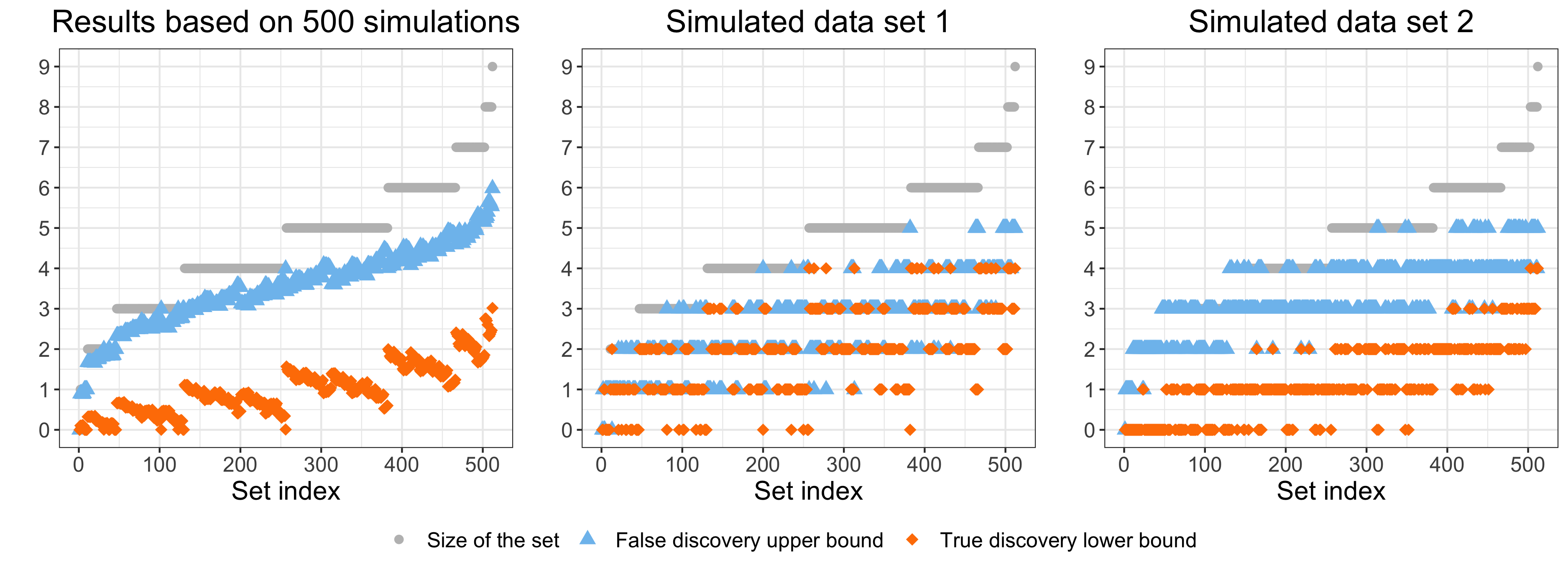
Figure 1: The false discovery upper bounds and true discovery lower bounds for all $512$ sets, as well as the size of each set. The first plot is the averaged result over $500$ simulations, and the second and third plots are the result based on two simulated datasets.

Over these $500$ simulations, the empirical probability of $P(|R\cap\mathcal{N}^{*}|\leq t_{\alpha}(R)\text{ for any }R\subseteq[m])$ is $0.988$, which is larger than $1-\alpha=0.95$, so the simultaneous guarantee (13) empirically holds. The average number of causal predictors is $4.144$, and the average number of discoveries of ICP is $0.52$. The first plot in Figure 1 shows the average false discovery upper bounds and true discovery lower bounds for all $512$ sets, as well as the size of each set. Note that the x-axis is only the index for each set, and we didn’t present which sets these indices refer to for simplicity. Compared to ICP, extra information can be obtained by looking at these bounds. For example, by looking at the true discovery lower bound of the set containing all predictors (with set index $512$), we know that, on average, there are about three true causal predictors in all nine predictors.

To better illustrate the usage of the simultaneous bounds in practice, we look at the results of two simulated datasets rather than the averaged results. These results are shown in the second and third plots of Figure 1, respectively.

For the first simulated dataset, the true causal predictors are $X_{1},X_{2},X_{3}$ and $X_{4}$. ICP discovers $X_{2}$ and $X_{3}$, meaning that with a probability larger than $0.95$, $X_{2}$ and $X_{3}$ are causal predictors. That is all the information we can get by using ICP. By looking at the simultaneous bounds (see the second plot in Figure 1), however, extra information can be obtained. For example, we can see that the sets with indices $131$ and $257$ has true discovery lower bounds $3$ and $4$, respectively. These two sets are $\{X_{1},X_{2},X_{3},X_{4}\}$ and $\{X_{1},X_{2},X_{3},X_{4},X_{5}\}$. Hence, we know that with probability larger than $0.95$, there are at least three causal predictors in $\{X_{1},X_{2},X_{3},X_{4}\}$, and at least four causal predictors in $\{X_{1},X_{2},X_{3},X_{4},X_{5}\}$. Note that the same information that both $X_{2}$ and $X_{3}$ are true causal predictors can also be obtained, because the true discovery lower bound for $\{X_{2},X_{3}\}$ (with set index $13$) is two.

For the second simulated dataset, the true causal predictors are $\{X_{1},X_{2},X_{3},X_{4},X_{5}\}$. ICP returns zero discoveries. In particular, the corresponding p-values (see (7)) for predictors are $1,1,1,1,\\ 0.848,0.329,1,1,1$. Hence, one can not get much information about the causal predictors by using ICP in this case. By looking at the simultaneous bounds (see the third plot in Figure 1), more information can be obtained. For example, we know that with a probability larger than $0.95$, there are at least one causal predictor in $\{X_{3},X_{7}\}$ (with set index $23$), at least two causal predictors in $\{X_{3},X_{5},X_{7},X_{8}\}$ (with set index $164$), at least three causal predictors in $\{X_{1},X_{3},X_{5},X_{7},X_{8},X_{9}\}$ (with set index $406$), and at least four causal predictors in $\{X_{1},X_{2},X_{3},X_{4},X_{5},X_{7},X_{8},X_{9}\}$ (with set index $503$).

4.2 Real data application

We look at a real dataset used in Stock et al., (2003) about the educational attainment of teenagers (Rouse,, 1995). This dataset contains information of $4739$ students from approximately 1100 US high schools, including gender, ethnicity, achievement test score, whether the father or mother is a college graduate, whether the family owns their home, whether the school is in an urban area, county unemployment rate, state hourly wage in manufacturing, average college tuition, whether the family income above 25000 per year, and region.

We follow Peters et al., (2016) to obtain two datasets of two environments, with $2231$ and $2508$ samples, respectively. The response variable $Y$ is a binary variable indicating whether the student attained a BA degree or higher. We use dummy variables to encode the factors in the dataset, resulting in $13$ predictors in total. The goal is to find the causal predictors of the response $Y$.

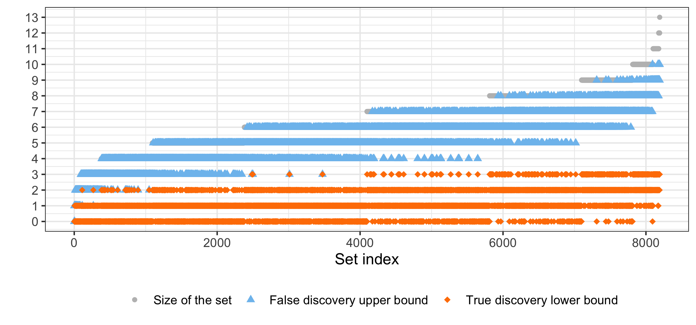
Figure 2: The false discovery upper bounds, true discovery lower bounds, and the size of set for all $8192$ sets based on the real data.

We first apply ICP with a significance level $\alpha=0.05$, returning one variable ‘score’ as the causal predictor. It seems reasonable that test score has a causal influence on whether the student would attain a BA degree or higher. We then calculate the simultaneous bounds for all $2^{13}=8192$ sets, and the results are shown in Figure 2. More information can be obtained by looking at these bounds. For example, by looking at the set with index $112$, we know that with a probability larger than $0.95$, there are at least two causal predictors in {‘score’, ’fcollege$\_$no’, ’mcollege$\_$no’}. It seems plausible that the true discovery lower bound is $2$ for this set, because the two variables of whether father or mother went to college are highly correlated, so it is difficult to distinguish between whether both are causal predictors or only one of them is.

Appendix A Supplementary material

A.1 Proof of Proposition 1

Proposition A.1.

For any $c\in(0,1)$, $P_{H^{*}_{0,i}}(p^{*}_{i}\leq c)\leq c$.

Proof.

When $H^{*}_{0,i}$ is true, we have $S^{*}\subseteq[m]\setminus\{i\}$ as $i\not\in S^{*}$, so $p^{*}_{i}=\max_{S\subseteq[m]\setminus\{i\}}p_{S}\geq p_{S^{*}}$. Therefore, for any $c\in(0,1)$,

$$P_{H^{*}_{0,i}}(p^{*}_{i}\leq c)\leq P_{H^{*}_{0,i}}(p_{S^{*}}\leq c)\leq c,$$

where the last inequality holds because $H_{0,S^{*}}(\mathcal{E})$ is true. ∎

A.2 Proof of Proposition 2

Proposition A.2.

For $\alpha\in(0,1)$, let $\tilde{S}(\mathcal{E})=\{i:\tilde{p}^{*}_{i}(\alpha)\leq\alpha\}$. Then $\tilde{S}(\mathcal{E})=\widehat{S}^{\text{ICP}}(\mathcal{E})$.

To prove Proposition 2, we first introduce the following lemma, which gives the relation between $\widehat{S}(\mathcal{E})=\{i:p^{*}_{i}(\alpha)\leq\alpha\}$ and $\widehat{S}^{\text{ICP}}(\mathcal{E})$.

Lemma A.1.

Assume that there exists $R\subseteq[m]$ such that $H_{0,R}(\mathcal{E})$ is not rejected. Let $\widehat{S}(\mathcal{E})=\{i:p^{*}_{i}(\alpha)\leq\alpha\}$. Then, $\widehat{S}(\mathcal{E})=\widehat{S}^{\text{ICP}}(\mathcal{E})$.

We first prove Lemma A.1.

Proof.

If $\widehat{S}(\mathcal{E})=\emptyset$, that is, $p^{*}_{i}=\max_{S\subseteq[m]\setminus\{i\}}p_{S}>\alpha$ for all $i\in[m]$, then we must have $\widehat{S}^{\text{ICP}}(\mathcal{E})=\emptyset$. Otherwise, if there exists some $j\in\widehat{S}^{\text{ICP}}(\mathcal{E})$, then for any $R$ whose corresponding $p_{R}>\alpha$, we must have $j\in R$ by the definition of $\widehat{S}^{\text{ICP}}(\mathcal{E})$. But $p^{*}_{j}=\max_{S\subseteq[m]\setminus\{j\}}p_{S}>\alpha$ implies that there exists some $R^{\prime}$ not containing $j$ and $p_{R^{\prime}}>\alpha$, which leads to a contradiction.

If $\widehat{S}^{\text{ICP}}(\mathcal{E})=\emptyset$, by the assumption in the proposition, there must exist some $R_{1}$ and $R_{2}$ such that $p_{R_{1}}>\alpha$, $p_{R_{2}}>\alpha$ and $R_{1}\cap R_{2}=\emptyset$. Then we must have $\widehat{S}(\mathcal{E})=\emptyset$. Otherwise, if there exists some $j\in\widehat{S}(\mathcal{E})$, that is, $p^{*}_{j}=\max_{S\subseteq[m]\setminus\{j\}}p_{S}\leq\alpha$, then in order for $p_{R_{1}}>\alpha$ and $p_{R_{2}}>\alpha$, both $R_{1}$ and $R_{2}$ must contain $j$, which contradicts the fact that $R_{1}\cap R_{2}=\emptyset$.

Now assume both $\widehat{S}(\mathcal{E})$ and $\widehat{S}^{\text{ICP}}(\mathcal{E})$ are non-empty.

If $i\in\widehat{S}^{\text{ICP}}(\mathcal{E})$, that is, for any $S$ such that $H_{0,S}(\mathcal{E})$ is not rejected (that is, $p_{S}>\alpha$), we have $i\in S$. So for any $R\subseteq[m]\setminus\{i\}$, $H_{0,R}(\mathcal{E})$ must be rejected, so $p^{*}_{i}=\max_{R\subseteq[m]\setminus\{i\}}p_{R}\leq\alpha$, which implies that $i\in\widehat{S}(\mathcal{E})$.

If $i\in\widehat{S}(\mathcal{E})$, we have $p^{*}_{i}=\max_{S\subseteq[m]\setminus\{i\}}p_{S}\leq\alpha$, which implies that for any $S$ not containing $i$, $H_{0,S}(\mathcal{E})$ must be rejected. So for any $R$ such that $H_{0,R}(\mathcal{E})$ is not rejected, we must have $i\in R$, which implies that $i\in\widehat{S}^{\text{ICP}}(\mathcal{E})$. ∎

Now we prove Proposition 2.

Proof.

If there exists some $R\subseteq[m]$ such that $H_{0,R}(\mathcal{E})$ is not rejected, that is, $p_{R}>\alpha$. Then $\tilde{p}^{*}_{i}(\alpha)=\max\{p^{*}_{i},\Pi_{S\subseteq[m]}\mathbbm{1}_{p_{S}\leq\alpha}\}=\max\{p^{*}_{i},0\}=p^{*}_{i}$, so $\tilde{S}(\mathcal{E})=\widehat{S}(\mathcal{E})=\widehat{S}^{\text{ICP}}(\mathcal{E})$ by Lemma A.1.

Now we consider the remaining case that $H_{0,S}(\mathcal{E})$ is rejected for all $S\subseteq[m]$, that is, $p_{S}\leq\alpha$ for all $S\subseteq[m]$. Then, we have $\widehat{S}^{\text{ICP}}(\mathcal{E})=\emptyset$ by definition, and $\tilde{p}^{*}_{i}(\alpha)=\max\{p^{*}_{i},\Pi_{S\subseteq[m]}\mathbbm{1}_{p_{S}\leq\alpha}\}=\max\{p^{*}_{i},1\}=1>\alpha$ for any $i\in[m]$. Hence $\tilde{S}(\mathcal{E})=\emptyset=\widehat{S}^{\text{ICP}}(\mathcal{E})$. ∎

A.3 Proof of Proposition 3

Proposition A.3.

For $\alpha\in(0,1)$, we have $P\left(\widehat{S}(\mathcal{E})\subseteq S^{*}\right)\geq 1-\alpha.$

Proof.

When $H_{0,S^{*}}(\mathcal{E})$ is not rejected, for any $i\not\in S^{*}$, we have $p^{*}_{i}=\max_{S\subseteq[m]\setminus\{i\}}p_{S}\geq p_{S^{*}}>\alpha$, so $i\not\in\widehat{S}(\mathcal{E})$. Hence, we have $\widehat{S}(\mathcal{E})\subseteq S^{*}$. Therefore,

$$P\left(\widehat{S}(\mathcal{E})\subseteq S^{*}\right)\geq P\left(H_{0,S^{*}}(\mathcal{E})\text{ is not rejected}\right)\geq 1-\alpha.$$

∎

A.4 Proof of Proposition 4

Proposition A.4.

For any $c\in(0,1)$, $P_{H^{*}_{0,S}}(p^{*}_{S}\leq c)\leq c$.

Proof.

When $H^{*}_{0,S}$ is true, we have $S^{*}\subseteq[m]\setminus S$ as $S\cap S^{*}=\emptyset$, so $p^{*}_{S}=\max_{I\subseteq[m]\setminus S}p_{I}\geq p_{S^{*}}$. Therefore, for any $c\in(0,1)$,

$$P_{H^{*}_{0,S}}(p^{*}_{S}\leq c)\leq P_{H^{*}_{0,S}}(p_{S^{*}}\leq c)\leq c.$$

∎

A.5 Proof of Theorem 1

Theorem A.1.

Let $\alpha\in(0,1)$, then

$$P(|R\cap\mathcal{N}^{*}|\leq t_{\alpha}(R)\text{ for any }R\subseteq[m])\geq 1-\alpha.$$

Proof.

For any $R\subseteq[m]$,

$$p^{*}_{R\cap\mathcal{N}^{*}}=\max_{I\subseteq[m]\setminus(R\cap\mathcal{N}^{*})}p_{I}\geq\max_{I\subseteq[m]\setminus\mathcal{N}^{*}}p_{I}=p^{*}_{\mathcal{N}^{*}}.$$

So if $p^{*}_{\mathcal{N}^{*}}>\alpha$, we have $p^{*}_{R\cap\mathcal{N}^{*}}>\alpha$, which implies that $|R\cap\mathcal{N}^{*}|\leq t_{\alpha}(R)$ by definition. Hence

$$P(|R\cap\mathcal{N}^{*}|\leq t_{\alpha}(R)\text{ for any }R\subseteq[m])\geq P(p^{*}_{\mathcal{N}^{*}}>\alpha).$$

In addition, we have

$$P(p^{*}_{\mathcal{N}^{*}}\leq\alpha)=P(\max_{I\subseteq[m]\setminus\mathcal{N}^{*}}p_{I}\leq\alpha)\leq P(p_{S^{*}}\leq\alpha)\leq\alpha,$$

or equivalently

$$P(p^{*}_{\mathcal{N}^{*}}>\alpha)\geq 1-\alpha,$$

which completes the proof. ∎

A.6 Proof of Proposition 5

Proposition A.5.

Let $S^{*}$ be the set of true causal predictors. Consider the desired case where only $H_{0,S^{*}}(\mathcal{E})$ is true, $p_{S^{*}}\sim U(0,1)$ and $p_{S}=0$ for any $S\neq S^{*}$. Then, for $p^{\prime}_{i}$ satisfying (15), there exists some $c^{*}\in(0,1)$ such that $P_{H^{*}_{0,i}}(p^{\prime}_{i}\leq c^{*})>c^{*}$.

Proof.

For any $i$ such that $H^{*}_{0,i}$ is true, we have $p^{*}_{i}=\max_{S\subseteq[m]\setminus\{i\}}p_{S}=p_{S^{*}}$.

Since $P_{H^{*}_{0,i}}(p^{\prime}_{i}<p^{*}_{i})>0$, there must exist some rational number $c^{*}\in(0,1)$ such that

$$P_{H^{*}_{0,i}}(p^{\prime}_{i}\leq c^{*}<p^{*}_{i})>0.$$ (16)

Then,

$$P_{H^{*}_{0,i}}(p^{\prime}_{i}\leq c^{*})$$

$$= P_{H^{*}_{0,i}}(p^{\prime}_{i}\leq c^{*},p^{\prime}_{i}<p^{*}_{i})+P_{H^{*}_{0,i}}(p^{\prime}_{i}\leq c^{*},p^{\prime}_{i}=p^{*}_{i})$$

$$= P_{H^{*}_{0,i}}(p^{\prime}_{i}\leq c^{*},p^{\prime}_{i}<p^{*}_{i}\leq c^{*})+P_{H^{*}_{0,i}}(p^{\prime}_{i}\leq c^{*}<p^{*}_{i})+P_{H^{*}_{0,i}}(p^{\prime}_{i}\leq c^{*},p^{\prime}_{i}=p^{*}_{i})$$

$$> P_{H^{*}_{0,i}}(p^{*}_{i}\leq c^{*},p^{\prime}_{i}<p^{*}_{i})+P_{H^{*}_{0,i}}(p^{*}_{i}\leq c^{*},p^{\prime}_{i}=p^{*}_{i})$$

$$= P_{H^{*}_{0,i}}(p^{*}_{i}\leq c^{*})$$

$$= P_{H^{*}_{0,i}}(p_{S^{*}}\leq c^{*})$$

$$= c^{*},$$

which completes the proof. ∎

References

- Benjamini and Hochberg, (1995) Benjamini, Y. and Hochberg, Y. (1995). Controlling the false discovery rate: a practical and powerful approach to multiple testing. Journal of the Royal statistical society: series B (Methodological), 57(1):289–300.
- Benjamini and Yekutieli, (2001) Benjamini, Y. and Yekutieli, D. (2001). The control of the false discovery rate in multiple testing under dependency. Annals of statistics, pages 1165–1188.
- Genovese and Wasserman, (2006) Genovese, C. R. and Wasserman, L. (2006). Exceedance control of the false discovery proportion. Journal of the American Statistical Association, 101(476):1408–1417.
- Goeman et al., (2021) Goeman, J. J., Hemerik, J., and Solari, A. (2021). Only closed testing procedures are admissible for controlling false discovery proportions. The Annals of Statistics, 49(2):1218–1238.
- Goeman and Solari, (2011) Goeman, J. J. and Solari, A. (2011). Multiple testing for exploratory research. Statistical Science, 26(4):584–597.
- Heinze-Deml et al., (2018) Heinze-Deml, C., Peters, J., and Meinshausen, N. (2018). Invariant causal prediction for nonlinear models. Journal of Causal Inference, 6(2).
- Kook et al., (2023) Kook, L., Saengkyongam, S., Lundborg, A. R., Hothorn, T., and Peters, J. (2023). Model-based causal feature selection for general response types. arXiv preprint arXiv:2309.12833.
- Lehmann and Romano, (2022) Lehmann, E. and Romano, J. P. (2022). Multiple testing and simultaneous inference. In Testing Statistical Hypotheses, pages 405–491. Springer.
- Marcus et al., (1976) Marcus, R., Eric, P., and Gabriel, K. R. (1976). On closed testing procedures with special reference to ordered analysis of variance. Biometrika, 63(3):655–660.
- Peters et al., (2016) Peters, J., Bühlmann, P., and Meinshausen, N. (2016). Causal inference by using invariant prediction: identification and confidence intervals. Journal of the Royal Statistical Society: Series B (Statistical Methodology), 78(5):947–1012.
- Pfister et al., (2019) Pfister, N., Bühlmann, P., and Peters, J. (2019). Invariant causal prediction for sequential data. Journal of the American Statistical Association, 114(527):1264–1276.
- Rouse, (1995) Rouse, C. E. (1995). Democratization or diversion? the effect of community colleges on educational attainment. Journal of Business & Economic Statistics, 13(2):217–224.
- Stock et al., (2003) Stock, J. H., Watson, M. W., et al. (2003). Introduction to econometrics, volume 104. Addison Wesley Boston.