Lessons Learned
Reproducibility, Replicability, and When to Stop

Abstract

While extensive guidance exists for ensuring the reproducibility of one’s own study, there is little discussion regarding the reproduction and replication of external studies within one’s own research. To initiate this discussion, drawing lessons from our experience reproducing an operational product for predicting tropical cyclogenesis, we present a two-dimensional framework to offer guidance on reproduction and replication. Our framework, representing model fitting on one axis and its use in inference on the other, builds upon three key aspects: the dataset, the metrics, and the model itself. By assessing the trajectories of our studies on this 2D plane, we can better inform the claims made using our research. Additionally, we use this framework to contextualize the utility of benchmark datasets in the atmospheric sciences. Our two-dimensional framework provides a tool for researchers, especially early career researchers, to incorporate prior work in their own research and to inform the claims they can make in this context.

1 Introduction

Should scientists focus their efforts on reproducing previous studies? The answer to this question seems straightforward—the reproduction of scientific studies has been a recurrent focus over concerns that published works may be irreproducible or irreplicable (Nichols et al., 2021; Hoffmann et al., 2021). Additionally, reproducibility of results is taken as evidence of scientific robustness across numerous domains (Gervais, 2021; Ahadi et al., 2016; Baker, 2016). In the atmospheric sciences, this is evidenced by data replication efforts (e.g., the ESGF Data Replication Project—(Cinquini et al., 2014)) and benchmark dataset requirements (e.g., “The availability of an existing solution […] will also enable the easy reproduction of published results to verify that the workflow is consistent.”, (Dueben et al., 2022)). However, the terms reproducibility and replicability themselves can be a source of confusion—the (US) National Academies note that depending on the field, what is meant by each of these two terms can be “inconsistent, or even contradictory” (NASEM, 2019), a fact that is echoed by others in the literature (Devezer et al., 2021). In light of the substantial efforts by the academies in guiding scientists’ endeavors to improve the reproducibility and replicability of their own works, let us borrow their definitions—1) Reproducibility entails obtaining consistent computational results using the same input data, computational steps, methods, code, and conditions of analysis; and 2) Replication entails obtaining consistent results across studies, aimed at answering the same scientific question, each of which has obtained its own data. Still, we note that reproduction and replication of work does not itself provide proof of a given claim (Baker, 2016; Goodman et al., 2016), but each plays an important role in science, and efforts towards them are laudable.

This begets the question of how to address reproducibility and replication in scientific works. While we can point to sources in the literature providing guidance in making researchers’ findings more reproducible (e.g., ; ; ; , ), we found limited guidance regarding the reproduction and replication of others’ work in one’s own research studies—motivating our study.

2 Lessons Learned from Predicting Tropical Cyclogenesis

Reproduction and replication are important, and I propose that we keep this in mind as we take a look at our case study, in which we aimed to apply modern machine learning techniques to a well-known problem in meteorology—the prediction of tropical cyclone formation, or “tropical cyclogenesis” (see S1:Scientific Motivation). We believed that interpreting such models could provide scientific insight into an aspect of tropical cyclones that has been described as both vexing and intractable (Emanuel, 2018). We wanted to select a well-established method as a baseline—assessing new models against well-established methods is, after all, generally the main interest of a study (Jolliffe and Stephenson, 2005)—and we thus selected the base study (Schumacher et al., 2009) for the 2014 Tropical Cyclone Formation Probability product (NOAA and CIRA, 2010). Taking inspiration from Devezer et al. (2021), we set up a number of definitions detailed in Section 4. Armed with these definitions, we begin by saying we want to develop a model $M$ through a study $\xi$ that depends in part on the inputs ($\mathbf{X}$) and model $M_{\text{\tiny BASE}}$ in the base study, i.e.:

$$\xi\sim\left({M,M_{\text{\tiny BASE}},\mathbf{X}}\right).$$ (1)

While we sampled our input variables from ECMWF’s European Reanalysis 5 (Hersbach et al., 2019) (ERA5 hereafter), we were aware that $M_{\text{\tiny BASE}}$ was not developed using $X$. After all, ERA5 was not available when $M_{\text{\tiny BASE}}$ was first developed, and $M_{\text{\tiny BASE}}$ instead relied on a combination of GFS analysis/reanalysis data and satellite data—henceforth denoted as $X_{BASE}$ (Schumacher et al., 2009). Furthermore, we knew that simply transferring the model—assuming all of the variables in $X_{BASE}$ used to fit $M_{\text{\tiny BASE}}$ were available in $X$—was not a straightforward task. This is evidenced by the rich literature on the subject of dataset shifts and generalization, including, e.g., Wang et al. (2022); Malinin et al. (2021); Quinonero-Candela et al. (2008). As such, we needed to develop a version of $M_{\text{\tiny BASE}}$ that was trained using samples taken from $X$—i.e., $M_{\text{\tiny BASE.ERA5}}$—and we reasoned that the best way to do so was to first faithfully reproduce $M_{\text{\tiny BASE}}$ (i.e., the hyperparameters $\mathbf{\theta_{hyper}}$ and trainable parameters $\mathbf{\theta_{train}}$ associated with $M_{\text{\tiny BASE}}$) to ensure that our understanding of the model was sufficient to train $M_{\text{\tiny BASE.ERA5}}$.

Despite the help of the authors of Schumacher et al. (2009), our attempts at reproducing the base study would undergo several complications. First, the model that was shared with us had been updated since the publication of Schumacher et al. (2009)—thus, this reference would be insufficient for our efforts. Though there was an AMS presentation highlighting part of the updates to the model (Schumacher et al., 2014) and the authors provided the original developmental dataset (i.e., $X_{BASE}$), the model was developed for operational use rather than publication and a number of developmental details were unavailable. In a sense, we were working off an incomplete set of schematics; noting that ignorance of model training choices is detrimental (McGovern et al., 2022). As a result, it would take numerous months to develop a working understanding of the model as it existed at the time (model details are given in S2:Base Model Details). We had access to performance metrics of the post-processed model (e.g., the Brier score, ROC curve, and reliability), but we were missing the fitting metric of the sub-model for classification (the confusion matrix of the LDA). Yet another obstacle we faced was one that is more frequently encountered—the original Linear Discriminant Analysis (LDA) model was developed with then commonly used Fortran libraries, while our efforts utilized Python equivalents (e.g., Scikit-Learn—Pedregosa et al. 2011). Subtle implementation differences (e.g., in the solvers used), lying in codebases too time-consuming to compare in depth, made it difficult to achieve the same LDA coefficients; noting here that since I lacked the original sub-model performance metrics, the coefficients were the target for my model reproduction efforts. We could be said to be trying to reproduce the model using a potentially different set of tools. And still we added another layer of complexity to our efforts —we wanted to find a way to improve the model. After all, we wanted to give the LDA approach the best shot in our comparisons—we believe that baselines should be made robust to produce fair comparisons (details on attempted improvements are given in S3:Proposed Improvements). We were simultaneously trying to develop the capacity to emulate our predecessors while also increasing the height of the bar. In summary: we were attempting to hit a blurry target with a model constructed using incomplete schematics and a potentially different set of tools, all while attempting to find ways to improve the model.

With our efforts described as such, it may be no surprise that they were not fruitful. While we could use the model to reproduce the images on the product website, training our own models resulted in algorithms that exhibited a wide variance in metrics depending on the data split. The model with our own attempts at improvement seemed to provide more stable results, but comparisons were within the standard deviations of the metrics as measured by our cross validation scheme. Our progress became so slow that we decided it no longer made sense to continue with these efforts, at which point we started to analyze where the project had gone awry. This led us to a strange realization: while there is plenty of literature offering guidance in ways to make your own work more reproducible and replicable, we were not aware of similar documents describing how to gauge the level of reproducibility and replicability of others’ works serving as the baseline in your study. This raises essential questions: How much effort should be allocated to replicability efforts? And how can one effectively guide and quantify replicability efforts to ensure rigor in the study’s conclusions?

3 A Short Guide to Reproduction and Replication

The level of reproduction and replication of previous work can have a significant impact on the scientific claims that can be made in light of said work. Thus, the aim of this work is to address a perceived lack of guidance with regard to gauging the extent of reproduction/replication of others’ work achieved in one’s own studies. Furthermore, we expect that methods for evaluating reproduction and replication can provide guidance in evaluating future projects, and potentially serve as an evaluation tool during review processes.

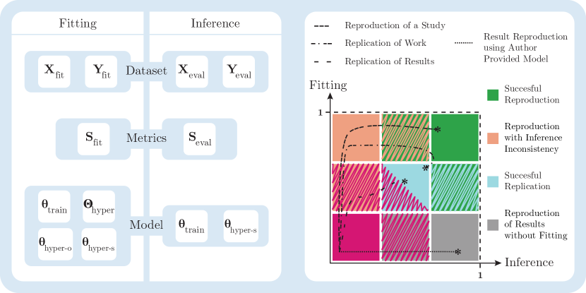
Figure 1: We introduce a two-component framework for assessing replication, employing distinct axes to represent the fitting and inference aspects. The y-axis (“Fitting”) evaluates the concordance in dataset, metrics, and parameters utilized for model training, while the x-axis (“Inference”) assesses the alignment in dataset, metrics, and parameters employed for model evaluation. Empirical scores guide the positioning along each axis, with the depicted paths on the right illustrating typical trajectories in research endeavors. $\bm{\theta}_{hyper-o}$ denotes the optimization hyperparameters, $\bm{\theta}_{hyper-s}$ denotes the structural hyperparameters (e.g., the depth, width, and type of a neural network’s layers), and $\bm{\Theta}_{hyper}$ denotes the searchable hyperparameter space. Other Variables are defined in the appendix.

For simplicity’s sake, we aim to quantify reproduction and replication using two axes, as depicted in Figure 1. The vertical axis represents the ability to fit a base model (e.g., the model described by Schumacher et al. (2009, 2014))—measured by one’s confidence in the reproduction of the fitting dataset, metrics, and model associated with the base study—represented by a value ranging from 0–1. In contrast, the horizontal axis represents the ability to use the model in inference mode to evaluate its performance—measured by one’s confidence in the reproduction of the evaluation dataset, metrics, and model—once again represented by a value ranging from 0–1. The definition of these axes provides a useful analytical tool, but we still lack a method for evaluating our position on the axes.

First, what precisely defines confidence in the equivalence of our datasets, metrics, and models can vary depending on our understanding of the research subject and the particularities of the question being addressed. In early research, for example, agreement on the sign of the coefficients associated with covariates in a linear model can already be ambitious. In light of this variance, ways to determine our position on these axes are not immediately apparent and thus evaluation of our positioning on these axes is something that must be considered per project. Still, in our hope to provide guidance to researchers we propose that one’s position along these axes be evaluated empirically using the questionnaire made available at github.com/msgomez06/RepoRepli—whose questions can be found in S4:Questionnaire.

In Figure 1 we further propose a set of curves describing what we consider are typical trajectories taken by researchers when undertaking research. Noting that the trajectories start in the red, bottom-left corner of the diagram, which represents a point in which the researcher is not yet familiar with the study and is not yet in possession of the pertinent datasets. For reproduction and replication studies, the trajectory continues with increasing confidence in the ability to produce an equivalent set of input and target samples (i.e., $\mathbf{X}_{fit}$ & $\mathbf{Y}_{fit}$), an equivalent set of fitting metrics $\mathbf{S}_{fit}$ (e.g., accuracy, recall, root mean square error), and thereby fit the model defined by a set of equivalent model hyperparameters $\bm{\theta}_{hyper}$, resulting in a set of trainable parameters $\bm{\theta}_{train}$ equivalent to those in the base study. We note that at this stage the path is in the orange, top-left corner of the diagram, where if the researcher would be unable to develop confidence in the use of the model in inference mode for evaluation purposes, this would be indicative of inconsistencies in the evaluation of the model in inference mode. Assuming the researcher is instead able to use the model in inference mode and develop confidence that the evaluation dataset and protocols are equivalent to those in the base study, their trajectory should move to the top-right corner, indicative of a successful reproduction procedure. If the aim of the research project is replication (e.g., to establish a framework’s robustness), the researcher moves from a regime in which they are confident that all aspects of the fitting and inference evaluation are equivalent, and makes modifications that decrease this degree of confidence. This includes, e.g.: changing the fitting and evaluation datasets by adding or removing covariates; changing the model hyperparameters used to make predictions; and changing the evaluation protocol to focus on different aspects of the predicted outcomes. We emphasize that these are idealized examples of trajectories - actual research trajectories will vary as projects progress.

Second, we propose that this two-axis framework (and the trajectory taken through it) can help inform the type of claims that can be made from one’s research. Let’s consider the AI-model baselines described by (Rasp et al., 2023), which are described as being trained on datasets covering a different number of years. While it is understandable that the models were not retrained for comparison—model training times ranged from 5.5 days on a single Nvidia A100 GPU to 4 weeks on 32 TPU v4 devices—this mismatch in training data results in a comparison between models that is less fair. This is pointed out by Rasp et al. (2023), who note that training on additional data results in improved performance. Figure 5 in Sweet et al. (2023) also demonstrates how a model’s skill can vary significantly depending on which year is used for evaluation. In our framework, we see that this relates to less confidence in $\mathbf{X}_{fit}$ being equivalent, independently of the inference dataset used. Furthermore, without a quantification of the uncertainty in $\mathbf{S}_{fit}$ and $\mathbf{S}_{eval}$, it becomes more difficult to compare the scores achieved by the models. Still, by providing a consistent evaluation framework including the dataset and metrics, Rasp et al. (2023) facilitate reproduction and replication studies.

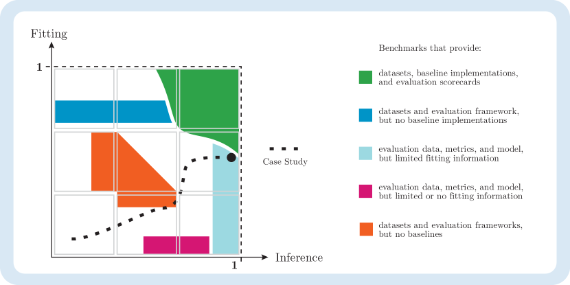
Figure 2: Benchmark datasets that provide baseline implementations and evaluation scorecards (green) allow users to start in the “successful reproduction” area. The absence of baseline implementation (dark blue) limits inference, while little (light blue) to no (pink) fitting information (light blue) prevents re-fitting of the model. The absence of baseline models (orange) prevents objective comparison to prior work. We note that benchmark datasets providing baselines. Note that the green section describes benchmark datasets fulfilling the first-order requirements and requirement 5 of the second-order requirements described by Dueben et al. (2022), while the orange section describes benchmark datasets fulfilling only the first-order requirements. This difference is due to the inclusion of trainable baselines for verifying workflows.

We can further use the framework to describe the advantages provided by benchmark datasets more generally, as shown in Figure 2. We start by considering the first-order and second-order requirements for benchmark datasets described by Dueben et al. (2022). The first four requirements focus on data access, problem definition, and evaluation metrics. The confidence provided by benchmark datasets thus allow researchers to start their trajectories in an advantageous position—the researchers position on the axes should be high considering the dataset confidence and metric confidence stemming from the use of a benchmark. Similarly, requirement 5 focuses on providing baselines. Quoting Dueben et al. (2022): ”The availability of an existing solution will facilitate the use of the dataset but will also enable the easy reproduction of published results to verify that the workflow is consistent.” We see here that providing a baseline that allows the verification of a consistent workflow means that researchers are able to begin in the top-right ”successful reproduction” area of the diagram, greatly facilitating replication studies. With requirements 6-8, we note one of the limitations of the two-axes framework: while the representation allows us to determine the confidence in our ability to reproduce and replicate a study, it does not include a measure of the quality of the dataset, evaluation protocol, and model. Dueben et al. (2022) define in these requirements for visualizations, diagnostics, physical consistency, and computational performance - all aspects that are independent of the reproduction and replication of base studies but rather focus on the rigor of the scientific question being addressed or the computational efficiency of the model implementation. Still, the framework shows clear advantages associated with using benchmark datasets in reproduction and replication efforts.

Finally, we take this opportunity to circle back to the case study presented in Section 2. We were able to reproduce the resulting maps from the base study well but hit a limit with our confidence in improving our ability to fit the model—depicted by the case study path in Figure 2. Looking back, perhaps our goals for confidence in the evaluation of the model were too high and unachievable in the context of trying to reproduce a production algorithm instead of the original study (i.e., Schumacher et al., 2009). Alternatively, we could have decided to not pursue a replication study and simply use the study as inspiration for the baseline while being clear that there were fundamental differences in our implementation versus the one used in production, limiting the claims we could make. Regardless, we believe that the limitations encountered in our case study could help other researchers in similar circumstances with their decision-making.

4 Conclusions

In conclusion, while making a study reproducible can be informed by checklists (e.g., those provided by ESIP Data Readiness Cluster (2022); Dueben et al. (2022)), we emphasize the need for a holistic approach when replicating an already-completed study. As a first step, we propose the use of a questionnaire that allows researchers to place themselves on the proposed two-dimensional representation of a study. The evaluation of our ability to reproduce and replicate the fitting of the model, as well as our ability to do the same for the evaluation of the model in inference mode, serves as a diagnosis to focus efforts for improvements to our approach at reproducing/replicating previous studies. Furthermore, carefully considering the aspects that we are able (or unable) to reproduce with regard to base studies can inform the types of claims we make after completing the study.

This underscores the utility of benchmark datasets in atmospheric science, which provide consistent datasets and evaluations to allow model comparison. This is especially important considering model sensibilities to spatiotemporal partitioning and the claims we can make as a result. By providing accessible datasets, metrics, and baseline models, study reproduction & replication become streamlined and lead to better scientific discussions.

1. There is a random variable $Y$ with discrete measurements $\bm{Y}_{obs}$,
   $\mathbf{Y}_{obs}\in\{y_{event},y_{non-event}\}$.

We believe that there are variables associated with the event that can be useful to predict event occurrences, and thus we say:

1. There is a random variable $\mathbf{X}$ with observed measurements $\mathbf{X}_{obs}$ that we believe can be used to predict $\bm{Y}_{obs}$

Having defined an event and an associated set of predictors, we want to find a model $M$ which uses a set of learnable parameters $\bm{\theta}_{learn}$ and the predictors $\mathbf{X}_{obs}$ to make a set of predictions $\mathbf{\hat{Y}}$ of the event.

1. $\mathbf{\hat{Y}}=\bm{M}\left(\mathbf{X}_{obs},\;\bm{\theta}_{learn}\right)$

Since parameters are learned from measurements, we obtain two or more independent samples of $\mathbf{X}$ and $\bm{Y}$ - a first time to obtain a model fitting set $\left\{\mathbf{X}_{fit},\mathbf{Y}_{fit}\right\}$ and a second time to obtain a model evaluation set $\left\{\mathbf{X}_{eval},\mathbf{Y}_{eval}\right\}$

1. $\mathbf{X}_{fit},\mathbf{X}_{eval}\in\mathbf{X},\quad\mathbf{Y}_{fit},\mathbf{Y}_{eval}\in\mathbf{Y},\quad\text{with}\quad\mathbf{X}_{fit}\cap\mathbf{X}_{eval}=\emptyset$

The model is defined by: 1) a set of structural hyperparameters $\bm{\theta}_{hyper-s}$ specifying the number of learnable parameters and the parameters are used to make the prediction (e.g., the depth, width, and type of layers in a neural network); 2) a method of fitting the model, specified by a set of optimization hyperparameters $\bm{\theta}_{hyper-o}$ controlling how learnable parameters should be adjusted during training (e.g., the batch size, learning rate, and optimization algorithm); and 3) the hyperparameter space $\bm{\Theta}_{hyper}$ considered when searching of the optimal values for $\bm{\theta}_{hyper-s}$ and $\bm{\theta}_{hyper-o}$.

1. $M\doteq F\left(\bm{\theta}_{hyper-o},\bm{\theta}_{hyper-s}\right),\quad\bm{\theta}_{hyper-o},\;\bm{\theta}_{hyper-s}\in\bm{\Theta}_{hyper}$

Having a model that makes predictions, we want to evaluate a distance between $\mathbf{\hat{Y}}$ and $\mathbf{Y}$, and thus use a set of metrics $\mathbf{S}$. We define two sets of $\mathbf{S}$—one used to adjust $\bm{\theta}_{learn}$ during model fitting, i.e., $\bm{S}_{fit}$; and one used to evaluate predictions made with $\mathbf{X}_{eval}$, i.e., $\mathbf{S}_{eval}$. $\mathbf{S}_{eval}$ generally includes or extends $\mathbf{S}_{fit}$, but it can be an independent set of evaluation metrics.

References

- Ahadi et al. (2016) Ahadi, A., A. Hellas, P. Ihantola, A. Korhonen, and A. Petersen, 2016: Replication in computing education research: researcher attitudes and experiences. Proceedings of the 16th Koli calling international conference on computing education research, 2–11.
- Baker (2016) Baker, M., 2016: 1,500 scientists lift the lid on reproducibility. Nature, 533 (7604).
- Carter et al. (2023) Carter, E., C. Hultquist, and T. Wen, 2023: Grrien analysis: A data science cheat sheet for earth scientists learning from global earth observations. Artificial Intelligence for the Earth Systems, 2 (2), 220 065, https://doi.org/10.1175/AIES-D-22-0065.1, URL https://journals.ametsoc.org/view/journals/aies/2/2/AIES-D-22-0065.1.xml.
- Cinquini et al. (2014) Cinquini, L., and Coauthors, 2014: The earth system grid federation: An open infrastructure for access to distributed geospatial data. Future Generation Computer Systems, 36, 400–417.
- Devezer et al. (2021) Devezer, B., D. J. Navarro, J. Vandekerckhove, and E. Ozge Buzbas, 2021: The case for formal methodology in scientific reform. Royal Society open science, 8 (3), 200 805.
- Dueben et al. (2022) Dueben, P. D., M. G. Schultz, M. Chantry, D. J. Gagne, D. M. Hall, and A. McGovern, 2022: Challenges and benchmark datasets for machine learning in the atmospheric sciences: Definition, status, and outlook. Artificial Intelligence for the Earth Systems, 1 (3), e210 002.
- Emanuel (2018) Emanuel, K., 2018: 100 years of progress in tropical cyclone research. Meteorological Monographs, 59, 15–1.
- ESIP Data Readiness Cluster (2022) ESIP Data Readiness Cluster, 2022: Checklist to Examine AI-readiness for Open Environmental Datasets. 10.6084/m9.figshare.19983722.v1, URL https://esip.figshare.com/articles/online˙resource/Checklist˙to˙Examine˙AI-readiness˙for˙Open˙Environmental˙Datasets/19983722.
- Gervais (2021) Gervais, W. M., 2021: Practical methodological reform needs good theory. Perspectives on Psychological Science, 16 (4), 827–843.
- Goodman et al. (2016) Goodman, S. N., D. Fanelli, and J. P. Ioannidis, 2016: What does research reproducibility mean? Science translational medicine, 8 (341), 341ps12–341ps12.
- Hersbach et al. (2019) Hersbach, H., and Coauthors, 2019: Global reanalysis: goodbye era-interim, hello era5. European Center for Meidum-Range Weather Forecasts, URL https://www.ecmwf.int/node/19027, 17-24 pp., 10.21957/vf291hehd7.
- Hoffmann et al. (2021) Hoffmann, S., F. Schönbrodt, R. Elsas, R. Wilson, U. Strasser, and A.-L. Boulesteix, 2021: The multiplicity of analysis strategies jeopardizes replicability: lessons learned across disciplines. Royal Society Open Science, 8 (4), 201 925.
- Jolliffe and Stephenson (2005) Jolliffe, I. T., and D. B. Stephenson, 2005: Comments on “discussion of verification concepts in forecast verification: A practitioner’s guide in atmospheric science”. Weather and Forecasting, 20 (5), 796–800.
- Malinin et al. (2021) Malinin, A., and Coauthors, 2021: Shifts: A dataset of real distributional shift across multiple large-scale tasks. Thirty-fifth Conference on Neural Information Processing Systems Datasets and Benchmarks Track (Round 2), URL https://openreview.net/forum?id=qM45LHaWM6E.
- McGovern et al. (2022) McGovern, A., I. Ebert-Uphoff, D. J. Gagne, and A. Bostrom, 2022: Why we need to focus on developing ethical, responsible, and trustworthy artificial intelligence approaches for environmental science. Environmental Data Science, 1, e6, 10.1017/eds.2022.5.
- Mullendore et al. (2020) Mullendore, G. L., M. S. Mayernik, and D. Schuster, 2020: Determining best practices for archiving and reproducibility of model data. 100th American Meteorological Society Annual Meeting, AMS.
- National Academies of Sciences, Engineering, and Medicine (2019) (NACEM) National Academies of Sciences, Engineering, and Medicine (NACEM), 2019: Reproducibility and Replicability in Science. The National Academies Press, Washington, DC, 10.17226/25303, URL https://nap.nationalacademies.org/catalog/25303/reproducibility-and-replicability-in-science.
- National Oceanic and Atmospheric Administration and Cooperative Institute for Research in the Atmosphere (CIRA)(2010)National Oceanic and Atmospheric Administration (NOAA), and Cooperative Institute for Research in the Atmosphere (CIRA) (NOAA) National Oceanic and Atmospheric Administration (NOAA), and Cooperative Institute for Research in the Atmosphere (CIRA), 2010: Tropical cyclone formation probability product description. URL https://web.archive.org/web/20230601220235/https://www.ssd.noaa.gov/PS/TROP/TCFP/description.html.
- Nichols et al. (2021) Nichols, J. D., M. K. Oli, W. L. Kendall, and G. S. Boomer, 2021: A better approach for dealing with reproducibility and replicability in science. Proceedings of the National Academy of Sciences, 118 (7), e2100769 118, 10.1073/pnas.2100769118, URL https://www.pnas.org/doi/abs/10.1073/pnas.2100769118, https://www.pnas.org/doi/pdf/10.1073/pnas.2100769118.
- Pedregosa et al. (2011) Pedregosa, F., and Coauthors, 2011: Scikit-learn: Machine learning in Python. Journal of Machine Learning Research, 12, 2825–2830.
- Quinonero-Candela et al. (2008) Quinonero-Candela, J., M. Sugiyama, A. Schwaighofer, and N. D. Lawrence, 2008: Dataset shift in machine learning. The MIT Press.
- Rasp et al. (2023) Rasp, S., and Coauthors, 2023: Weatherbench 2: A benchmark for the next generation of data-driven global weather models. 2308.15560.
- Schumacher et al. (2009) Schumacher, A. B., M. DeMaria, and J. A. Knaff, 2009: Objective estimation of the 24-h probability of tropical cyclone formation. Weather and Forecasting, 24 (2), 456–471.
- Schumacher et al. (2014) Schumacher, A. B., M. DeMaria, J. A. Knaff, and H. Syed, 2014: Updates to the nesdis tropical cyclone formation probability product, URL https://ams.confex.com/ams/31Hurr/webprogram/Paper244172.html, 31st Conference on Hurricanes and Tropical Meteorology.
- Stall et al. (2023) Stall, S., and Coauthors, 2023: Ethical and responsible use of ai/ml in the earth, space, and environmental sciences . 10.22541/essoar.168132856.66485758/v1, URL http://dx.doi.org/10.22541/essoar.168132856.66485758/v1.
- Sweet et al. (2023) Sweet, L., C. Müller, M. Anand, and J. Zscheischler, 2023: Cross-validation strategy impacts the performance and interpretation of machine learning models. Artificial Intelligence for the Earth Systems, 2 (4), e230 026, https://doi.org/10.1175/AIES-D-23-0026.1, URL https://journals.ametsoc.org/view/journals/aies/2/4/AIES-D-23-0026.1.xml.
- Wang et al. (2022) Wang, J., and Coauthors, 2022: Generalizing to unseen domains: A survey on domain generalization. IEEE Transactions on Knowledge and Data Engineering.