The role of anharmonicity in single-molecule spin-crossover

Abstract

We exploit the system-bath paradigm to investigate anharmonicity effects of vibrations on spin-crossover (SCO) in a single molecule. Focusing on weak coupling, we use the linear response approximation to deal with the vibrational bath and propagate the Redfield master equation to obtain the equilibrium high spin fraction. We take both the anharmonicity in the bath potentials and the nonlinearity in the spin-vibration coupling into account and find a strong interplay between these two effects. Further, we show that the SCO in a single molecule is always a gradual transition and the anharmonicity-induced phonon drag greatly affects the transition behavior.

I Introduction

The ions’ 3$d$ orbitals in first-row transition metal complexes, which assume the electronic configuration 3$d^{4}$-3$d^{7}$, are split into bonding and antibonding ones by ligand field interaction Cavallini (2012). The splitting and the electron pairing energies are generally small and of the same order of magnitude, so that the effects of the Aufbau principle and the Hund’s rules are competitive. Under external perturbations, such as temperature change Denisov et al. (2021); Bronisz (2007); Shongwe et al. (2007), light irradiation Hauser (1986); Gütlich et al. (1994); Enachescu et al. (2002), pressure Molnár et al. (2003); Cowan et al. (2012), magnetic field Qi et al. (1983); Bousseksou et al. (2002), and electric field Prins et al. (2011), electrons may jump between bonding and antibonding orbitals due to the spin-orbit coupling, resulting in transition between the high-spin (HS) and the low-spin (LS) states. Such a spin-crossover (SCO) Takahashi (2018); Brooker (2015); Nakashima et al. (2018); Bousseksou et al. (2011) is usually accompanied by changes in magnetic moment, color Kahn et al. (1992), structure, dielectric constant Bousseksou et al. (2003), and even catalytic capacity Zhong et al. (2018). Because of the rich physics and phenomena, SCO has wide potential applications in molecular switches Bhandary et al. (2021), memory devices Kahn and Martinez (1998), sensors Linares et al. (2012), actuators Molnár et al. (2018) and has aroused extensive research interests.

Among various SCO phenomena, the thermal-induced ones Denisov et al. (2021) are of special interest, in which energy splitting between the HS and LS states are close to the thermal energy. In practical applications, the transition is required to be abrupt and occur at room temperature (roughly equivalent to 200 cm^-1). In this case the vibrations will play a key role due to the energy matching Ronayne et al. (2006); Zhang (2014). Various models have been proposed to understand the role of vibrations, including the Ising model extended with lattice vibration Zimmermann and König (1977), the atom-phonon model Nasser et al. (2011), and the “stretching and bending” model Ye et al. (2015).

Note that in metal-organic compounds, vibrations often assume strong anharmonicity due to the presence of hydrogen bonding or other intermolecular interactions. Shelest studied the thermodynamics of SCO with an anharmonic model and revealed that anharmonicity is one important parameter controlling the SCO transition Shelest et al. (2016). Nicolazzi et al. used the Lennard-Jones potential to model intermolecular interactions and found that anharmonicity can reduce the transition temperature and make the HS state more stable Nicolazzi et al. (2008, 2013); Mikolasek et al. (2017). These authors further demonstrated that anharmonicity in intermolecular interactions is pivotal to understand SCO in nanostructures which allows atoms to undergo large displacements away from their equilibrium positions Fahs et al. (2023). Boukheddaden proposed an anharmonic coupling model and showed that change in anharmonicity drastically alters the SCO transition Boukheddaden (2004). However, there are controversial conclusions in the literature. For instance, Wu et al. performed density functional theory calculations for the effects of anharmonicity on the zero-point energy and the entropy in Fe(II) and Fe(III) complexes and found a rather small contribution to SCO Wu et al. (2019).

In real systems, the anharmonic effects are interplayed by the many-body interaction, nonperturbative effects of dissipation and even the non-Markovianity. In order to obtain a clear picture of the anharmonic effect itself, here we adopt an anharmonic bath model in the open system paradigm and focus on the weak spin-vibration coupling. A numerical exact simulation of such a nonlinear dissipation system is expansive. For the weak dissipation under study, we can approximate the bath with the anharmonic influence functional approach suggested by Makri et al. Ilk and Makri (1994); Makri (1999a, b). Eventually, the anharmonic influence functional approach maps the anharmonic bath to a harmonic one with the help of an effective spectral density function. After doing so, we can follow the master equation approach developed for the linear dissipation to investigate single-molecule SCO. Note that simulations of SCO with master equation was recently used by Orlov et al. Orlov et al. (2021, 2022).

At first glance the use of a nonlinear bath model is ad hoc because in the open system paradigm the bath is always linear at any given temperature. Note that the dissipation theory is a phenomenological description for physics of open systems based on the quantum fluctuation-dissipation theorem Mori (1965); Kubo (1966). One of the key points is the system-bath separation which implies that the system-bath interaction is weak and the effect of a single bath mode on the system is negligibly small. A mode strongly couples to the system cannot be considered as a part of the bath and should be included in the system. The effect of the bath, therefore, is a collective behavior and the system only feels the overall fluctuation of its bath which is characterized by its spectral density function. In this case the central limit theorem assures a Gaussian statistics for the bath fluctuation, which can be reproduced with the linear-dissipation Caldeira-Leggett model Caldeira and Leggett (1981). This framework, however, only holds at a fixed temperature and the spectral density functions at different temperatures in principle are not necessarily the same. In reality, all baths, especially for low-dimensional and molecular systems, are intrinsically anharmonic. The use of linear dissipation for simulating physics of an anharmonic system will have to adopt a different spectral density function, hence a different bath, for each temperature and therefore loses the predictive power for any temperature-dependent behavior. A remedy is the above-mentioned nonlinear dissipation model, in which the same bath is used to consistently yield the effective spectral density functions for all temperatures.

The rest of the paper are organized as follows. In Sec. II, we outline the anharmonic influence functional method in the linear response regime. In Sec. III, we present calculations with different anharmonic settings to check their effects on SCO. A concise summary is provided in Sec. IV.

II Theoretical model

Here we will discuss the anharmonic effects without considering the Duschinsky rotation and mode-mode coupling. Up to the fourth-order expansion of the vibrational potential curves, we have the following Hamiltonian

$$\hat{H}_{tot}=\begin{pmatrix}\epsilon_{L}+\hat{H}_{vib}^{(L)}&-\frac{\lambda}{2}\\ -\frac{\lambda}{2}&\epsilon_{H}+\hat{H}_{vib}^{(H)}\end{pmatrix},$$ (1)

where $\lambda$ is the spin-orbital coupling, $\epsilon_{S}$ are the electronic energy and $\hat{H}_{vib}^{(S)}=\sum_{j}\Big{\{}\frac{\hat{p}_{j}^{2}}{2m_{j}}+$ $v^{(S)}_{j,1}x_{j}+v^{(S)}_{j,2}x_{j}^{2}+v^{(S)}_{j,3}x_{j}^{3}+v^{(S)}_{j,4}x_{j}^{4}\Big{\}}$ with $S=L$ and $H$ corresponding to the LS and HS states, respectively. This model Hamiltonian can be extracted from ab initio vibrational analysis at the LS and HS states followed with energy calculations for geometries displaced along the normal modes Giese et al. (2006). Here for simplicity, we further assume that the LS and HS states have the same anharmonicity, that is, $v_{j,3}^{(L)}=v_{j,3}^{(H)}$ and $v_{j,4}^{(L)}=v_{j,4}^{(H)}$.

The Hamiltonian in Eq. (1) can be re-expressed in terms of the system-plus-bath model

$$\hat{H}_{tot}=\hat{H}_{s}+\hat{H}_{b}+\hat{H}_{sb}.$$ (2)

Here we set the Planck constant $\hbar$ and the Boltzmann constant $k_{B}$ to unity. The Hamiltonian for a two-state system in Eq. (2) can be represented as $\hat{H}_{s}=-\frac{\Delta}{2}{\sigma}_{z}-\frac{\lambda}{2}{\sigma}_{x}$, where $\Delta=\epsilon_{H}-\epsilon_{L}$ is the energy bias between LS and HS states and ${\sigma_{z}}/{\sigma_{x}}$ are the Pauli matrices. Meanwhile, the Hamiltonian for the thermal bath is given by $\hat{H_{b}}=\sum_{j}[\hat{p}_{j}^{2}/(2m_{j})+V_{j}(\hat{x}_{j})]$, where $V_{j}(\hat{x}_{j})=\frac{1}{2}m_{j}\omega_{j}^{2}x_{j}^{2}(1+b_{j}\sqrt{\omega_{j}}x_{j}+a_{j}\omega_{j}x_{j}^{2})$ is the potential of the thermal bath, with $a_{j}$ and $b_{j}$ being coefficients characterizing bath anharmonicity. The Hamiltonian for the system-bath interaction is $\hat{H}_{sb}=\sigma_{z}\sum_{j}c_{j}(\hat{o}_{j}-\langle\hat{o}_{j}\rangle)$, where $c_{j}$ denotes the coupling constant between the system and the environment, the operator $\hat{o}_{j}=\hat{x}_{j}+\kappa_{j}\sqrt{\omega_{j}}\hat{x}_{j}^{2}$ with $\kappa_{j}$ being the nonlinear strength in the spin-vibration coupling, and $\langle\hat{o}_{j}\rangle=\textrm{Tr}[\hat{o}_{j}e^{-\beta\hat{H}_{b}}]/\textrm{Tr}e^{-\beta\hat{H}_{b}}$ denotes the equilibrium expectation of the operator $\hat{o}_{j}$.

Utilizing the linear response approximation of the bath, the effect of the bath is given by the correlation function Ilk and Makri (1994); Makri (1999a, b)

$$\alpha(t)=\frac{1}{\pi}\int_{0}^{\infty}\mathrm{d}\omega J_{\beta}(\omega)[\coth(\frac{\beta\omega}{2})\cos\omega t-i\sin\omega t],$$ (3)

where $\beta={1}/{T}$ with $T$ being the temperature, and $J_{\beta}(\omega)$ is the effective spectral density function

$$J_{\beta}(\omega)=\sum_{j,m,n}\frac{c_{j}^{2}\pi}{4Z_{j}}(e^{-\beta\epsilon_{n}^{(j)}}-e^{-\beta\epsilon_{m}^{(j)}})|o_{m,n}^{(j)}|^{2}\delta(\omega-\omega_{mn}^{(j)}).$$ (4)

Here $j$ is the index of the bath mode, $\epsilon_{n}^{(j)}$ denotes the ${n}$th eigen-energy, $Z_{j}$ represents the partition function, and $\omega_{mn}^{(j)}$ stands for the transition frequency for $m\to n$. In order to focus on anharmonic effects and avoid its interplay with other effects, we stick to the weak spin-vibration coupling and use the Redfield equation to obtain the equilibrium expectation

$$\frac{\mathrm{d}\hat{\rho}(t)}{\mathrm{d}t}={i}[\hat{\rho}(t),\hat{H}_{s}]-[{\sigma}_{z},(\hat{\Xi}\hat{\rho}(t)-\hat{\rho}(t)\hat{\Xi}^{\dagger})],$$ (5)

where the operator $\hat{\Xi}$ is defined as

$$\hat{\Xi}=\int_{0}^{\infty}\mathrm{d}\tau\alpha(\tau)e^{-{i}\hat{H}_{s}\tau}{\sigma}_{z}e^{{i}\hat{H}_{s}\tau}.$$ (6)

III Numerical results

Because a universal theory for the nonlinear dissipation is not available, we have to adopt a discretized description for the anharmonic bath Wang and Thoss (2007). To this end, we determine the parameters $c_{j}$ and $\omega_{j}$ upon discretizing the spectral density function $J_{\iota}({\omega})=\eta\omega\exp({-\omega/\omega_{c}})$ with 20 000 modes, where $\eta$ is the linear dissipation strength and $\omega_{c}$ is the high frequency cutoff. For the anharmonic coefficients, we set $a_{j}=\omega_{c}/({2\omega_{j}x_{j,-}x_{j,+}})$; $b_{j}=-2\sqrt{\omega_{c}}(x_{{}_{j,-}}+x_{{}_{j,+}})/(3\sqrt{\omega_{j}}x_{{}_{j,-}}x_{{}_{j,+}})$, where $x_{j,\pm}=f(\omega_{j}/\omega_{c})(1\pm 0.2\sqrt{1-1.6\omega_{j}/{\omega_{c}}})$ with $f(u)=\alpha(8u^{2}+1/32u^{2}+\gamma)$. Here $\alpha$ and $\gamma$ are two parameters controlling anharmonicity. Under these conditions, the bath modes with $\omega_{j}<\omega_{c}/1.6$ assume a double-well potential.

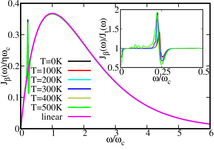
Figure 1: Effective spectral density function at different temperatures. The parameters in the nonlinear disspation part are $a_{j}=0.0043253\omega_{j}^{3}/((15+\omega_{j})(1-31.52\omega_{j}^{2}+256\omega_{j}^{4})^{2})$, $b_{j}=-0.49020\omega_{j}^{3/2}/((15+\omega_{j})(1-31.52\omega_{j}^{2}+256\omega_{j}^{4}))$, and $\kappa_{j}=0$. The parameters $c_{j}$ and $\omega_{j}$ for the linear part is determined by discretizing the spectral density $J_{\iota}(\omega)=0.05\omega\exp(-\omega/\omega_{c})$ with 20 000 modes. Check text for details about the Hamiltonian.

Here we set $\Delta=300$ K, $\lambda=50$ meV, $\eta=0.05$, $\omega_{c}=800$ cm^-1, $\alpha=1360$, and $\gamma=-0.985$. The parameters $\kappa_{j}$ will be set to the same value for all vibration, varying from 0 to 0.05 in step of 0.01. The calculated correlation functions for temperatures from 0 K to 500 K with intervals of 10 K are substituted into the Redfield equation to obtain the equilibrium distributions.

In Fig. 1 we present the effective spectral density functions for temperatures from 0 K to 500 K in step of 100 K. In the simulations, we first calculate the bath correlation function and perform the Fourier transform of its imaginary part to obtain the effective spectral density functions. For comparison we also plot the ratio ${J_{\beta}(\omega)}/{J_{\iota}(\omega)}$. As illustrated in Fig. 1, we observe that the effective spectral density function becomes temperature-dependent and deviates from the linear one. The overwhelming feature is that a sharp peak appears around $\omega=0.22\omega_{c}$ besides the original peak of the linear spectral density function. The anharmonic results merge to linear dissipation when $\omega>0.4\omega_{c}$.

We now discuss the effect of the anharmonicity in the bath potentials without the nonlinearity in the spin-vibration coupling. The results with linear dissipation are also presented. As shown in Fig. 2, with the anharmonic model, the HS fraction first decreases and then gradually increases with temperature. Even at a temperature as high as 500 K, the HS fraction is still less than one half. The harmonic model assumes roughly the same trend as the anharmonic one. However, subtle differences exist between the two trends, mainly in the temperature range from 100 K to 300 K, which is exactly the region in which the effective spectral density function deviates from its linear counterpart. It seems that the presence of the anharmonicity in the bath potential alone slows down the LS to HS transition. For comparison we show the results obtained from the Boltzmann distribution. It is interesting to note that even for such a weak dissipation, the results from quantum master equation are significantly different from the Boltzmann distribution.

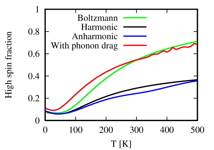
Figure 2: The effects of the anharmonicity in the bath potential on SCO. Boltzmann: Results given by the Boltzmann distribution; Harmonic: Equilibrium results of the Redfield equation with $a_{j}=0$, $b_{j}=0$, and $\kappa_{j}=0$; Anharmonic: Equilibrium results with anharmonicity in the bath potential only; With phonon drag: The thermal average $\langle\hat{o}_{j}\rangle$ is included in energy splitting. Parameters $\kappa_{j}$, $a_{j}$, and $b_{j}$ for the latter two are the same as that in Fig. 1.

Next we investigate the effect of the nonlinearity in the spin-vibration coupling without the potential anharmonicity. The results are shown in Fig. 3, which depicts the same overall trend as that in Fig. 2. For different nonlinear intensities characterized with $\kappa$, the differences are pretty small and only obvious between 100 K and 300 K.

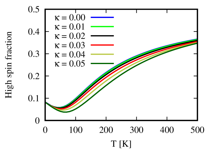
Figure 3: The effects of nonlinear spin-vibration coupling with harmonic bath potential. The parameter $\kappa_{j}$ are the same for all vibrations.

In the presence of both the anharmonicity in the bath potential and the nonlinearity in spin-vibration coupling, there may have strong interplay between these two effects. As shown in Fig. 4, now the temperature dependence are much more significant than that in Figs. 2 and 3, especially in the temperature range from 100 K to 300 K. With such an interplay, the HS fraction changes much abrupter with temperature for stronger nonlinear spin-vibration coupling.

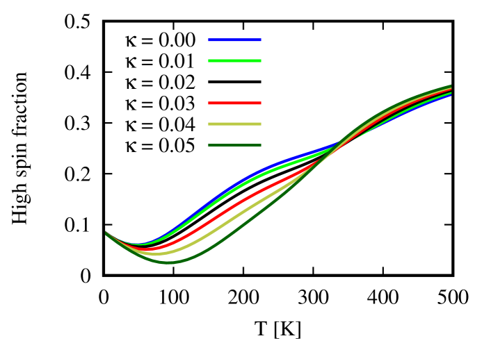
Figure 4: The interplay of the nonlinearity in the spin-vibration coupling and the anharmonicity in the potential. Anharmonic parameters $a_{j}$ and $b_{j}$ are the same as that in Fig.1.

Strictly speaking the energy splitting for the nonlinear dissipation model Eq. (2) is $\Delta=\epsilon_{H}-\epsilon_{L}+\sum_{j}c_{j}\langle\hat{o}_{j}\rangle$. For anharmonic potentials, the thermal equilibrium expectation of the position changes with temperature. Such a temperature-dependent equilibrium drift will cause an additional energy splitting in SCO. To characterize this phonon drag effect, we set all $c_{j}$ coefficients to positive in the bath discretization and add the thermal average $\sum_{j}c_{j}\langle\hat{o}_{j}\rangle$ to $\Delta$. Note that in calculating the thermal average $\langle\hat{o}_{j}\rangle$, the quadratic term $\hat{x}^{2}_{j}$ always assumes a temperature-dependent result. In order to simplify the analysis and focus on the phonon drag effect we use $\kappa=0$ to exclude the effect of nonlinear spin-vibration coupling. The corresponding results is demonstrated in Fig. 2, which shows that the phonon drag leads to a more pronounced temperature-dependence of the HS fraction.

IV Summary

In metal-organic compounds, vibrations may assume strong anharmonicity. In order to take account of the anharmonicity effect on the temperature-induced SCO, a linear dissipation model has to adopt a separate spectral density function at each temperature and thus fails to describe the temperature-dependent transition. Here an anharmonic vibrational bath model was used to simulate single-molecule SCO. With the linear response approximation, we were able to obtain the effective spectral density functions for all temperatures consistently with the same bath that can be extracted from ab initio calculations. To scrutinize the anharmonicity effect itself, we focused on the weak spin-vibration coupling to avoid further complications caused by strong interaction. Propagating the Redfield equation to sufficiently long time, we obtained the equilibrium distribution of the spin. We found a strong interplay between anharmonicity in the bath potential and nonlinearity in the spin-vibration coupling. We also demonstrated that the phonon drag drastically affects SCO and makes the transition much abrupter.

References

- Cavallini (2012) M. Cavallini, Phys. Chem. Chem. Phys. 14, 11867 (2012).
- Denisov et al. (2021) G. Denisov, V. V. Novikov, S. A. Belova, A. Belov, E. Melnikova, R. Aysin, Y. Z. Voloshin, and Y. V. Nelyubina, Cryst. Growth Des. 21, 4594 (2021).
- Bronisz (2007) R. Bronisz, Inorg. Chem. 46, 6733 (2007).
- Shongwe et al. (2007) M. S. Shongwe, B. A. Al-Rashdi, H. Adams, M. J. Morris, M. Mikuriya, and G. R. Hearne, Inorg. Chem. 46, 9558 (2007).
- Hauser (1986) A. Hauser, Chem. Phys. Lett. 124, 543 (1986).
- Gütlich et al. (1994) P. Gütlich, A. Hauser, and H. Spiering, Angew. Chem. Int. Ed. 33, 2024 (1994).
- Enachescu et al. (2002) C. Enachescu, U. Oetliker, and A. Hauser, J. Phys. Chem. B 106, 9540 (2002).
- Molnár et al. (2003) G. Molnár, V. Niel, J.-A. Real, L. Dubrovinsky, A. Bousseksou, and J. J. McGarvey, J. Phys. Chem. B 107, 3149 (2003).
- Cowan et al. (2012) M. G. Cowan, J. Olguín, S. Narayanaswamy, J. L. Tallon, and S. Brooker, J. Am. Chem. Soc. 134, 2892 (2012).
- Qi et al. (1983) Y. Qi, E. W. Müller, H. Spiering, and P. Gütlich, Chem. Phys. Lett. 101, 503 (1983).
- Bousseksou et al. (2002) A. Bousseksou, K. Boukheddaden, M. Goiran, C. Consejo, M.-L. Boillot, and J.-P. Tuchagues, Phys. Rev. B 65, 172412 (2002).
- Prins et al. (2011) F. Prins, M. Monrabal-Capilla, E. A. Osorio, E. Coronado, and H. S. J. van der Zant, Adv. Mater. 23, 1545 (2011).
- Takahashi (2018) K. Takahashi, Inorganics 6, 32 (2018).
- Brooker (2015) S. Brooker, Chem. Soc. Rev. 44, 2880 (2015).
- Nakashima et al. (2018) S. Nakashima, M. Kaneko, K. Yoshinami, S. Iwai, and H. Dote, Hyperfine Interact. 239, 1 (2018).
- Bousseksou et al. (2011) A. Bousseksou, G. Molnár, L. Salmon, and W. Nicolazzi, Chem. Soc. Rev. 40, 3313 (2011).
- Kahn et al. (1992) O. Kahn, J. Kröber, and C. Jay, Adv. Mater. 4, 718 (1992).
- Bousseksou et al. (2003) A. Bousseksou, G. Molnár, P. Demont, and J. Menegotto, J. Mater. Chem. 13, 2069 (2003).
- Zhong et al. (2018) W. Zhong, Y. Liu, M. Deng, Y. Zhang, C. Jia, O. V. Prezhdo, J. Yuan, and J. Jiang, J. Mater. Chem. A 6, 11105 (2018).
- Bhandary et al. (2021) S. Bhandary, J. M. Tomczak, and A. Valli, Nanoscale Adv. 3, 4990 (2021).
- Kahn and Martinez (1998) O. Kahn and C. J. Martinez, Science 279, 44 (1998).
- Linares et al. (2012) J. Linares, E. Codjovi, and Y. Garcia, Sensors 12, 4479 (2012).
- Molnár et al. (2018) G. Molnár, S. Rat, L. Salmon, W. Nicolazzi, and A. Bousseksou, Adv. Mater. 30, 1703862 (2018).
- Ronayne et al. (2006) K. L. Ronayne, H. Paulsen, A. Höfer, A. C. Dennis, J. A. Wolny, A. I. Chumakov, V. Schünemann, H. Winkler, H. Spiering, A. Bousseksou, P. Gütlich, A. X. Trautwein, and J. J. McGarvey, Phys. Chem. Chem. Phys. 8, 4685 (2006).
- Zhang (2014) Y. Zhang, J. Chem. Phys. 141, 214703 (2014).
- Zimmermann and König (1977) R. Zimmermann and E. König, J. Phys. Chem. Solids 38, 779 (1977).
- Nasser et al. (2011) J. A. Nasser, S. Topçu, L. Chassagne, M. Wakim, B. Bennali, J. Linares, and Y. Alayli, Eur. Phys. J. B 83, 115 (2011).
- Ye et al. (2015) H.-Z. Ye, C. Sun, and H. Jiang, Phys. Chem. Chem. Phys. 17, 6801 (2015).
- Shelest et al. (2016) V. V. Shelest, A. V. Khristov, and G. G. Levchenko, Low Temp. Phys. 42, 505 (2016).
- Nicolazzi et al. (2008) W. Nicolazzi, S. Pillet, and C. Lecomte, Phys. Rev. B 78, 174401 (2008).
- Nicolazzi et al. (2013) W. Nicolazzi, J. Pavlik, S. Bedoui, G. Molnár, and A. Bousseksou, Eur. Phys. J. Spec. Top. 222, 1137 (2013).
- Mikolasek et al. (2017) M. Mikolasek, W. Nicolazzi, F. Terki, G. Molnár, and A. Bousseksou, Chem. Phys. Lett. 678, 107 (2017).
- Fahs et al. (2023) A. Fahs, S. Mi, W. Nicolazzi, G. Molnár, and A. Bousseksou, Adv. Phys. Res. 2, 2200055 (2023).
- Boukheddaden (2004) K. Boukheddaden, Prog. Theor. Phys. 112, 205 (2004).
- Wu et al. (2019) J. Wu, C. Sousa, and C. de Graaf, Magnetochemistry 5, 49 (2019).
- Ilk and Makri (1994) G. Ilk and N. Makri, J. Chem. Phys. 101, 6708 (1994).
- Makri (1999a) N. Makri, J. Phys. Chem. B 103, 2823 (1999a).
- Makri (1999b) N. Makri, J. Chem. Phys. 111, 6164 (1999b).
- Orlov et al. (2021) Y. S. Orlov, S. V. Nikolaev, A. I. Nesterov, and S. G. Ovchinnikov, J. Exp. Theor. Phys. 132, 399 (2021).
- Orlov et al. (2022) Y. S. Orlov, S. V. Nikolaev, and S. G. Ovchinnikov, arXiv: 2211.01300 (2022).
- Mori (1965) H. Mori, Prog. Theo. Phys. 33, 423 (1965).
- Kubo (1966) R. Kubo, Rep. Prog. Phys. 29, 255 (1966).
- Caldeira and Leggett (1981) A. O. Caldeira and A. J. Leggett, Phys. Rev. Lett. 46, 211 (1981).
- Giese et al. (2006) K. Giese, M. Petković, H. Naundorf, and O. Kühn, Phys. Rep. 430, 211 (2006).
- Wang and Thoss (2007) H. Wang and M. Thoss, J. Phys. Chem. A 111, 10369 (2007).