Inference on testing the number of spikes in a high-dimensional generalized two-sample spiked model and its applicationsDandan Jiang was supported by NSFC Grant No.11971371 and the Fundamental Research Funds for the Central Universities.

Abstract

Two-sample spiked model is an important issue in multivariate statistical inference. This paper focuses on testing the number of spikes in a high-dimensional generalized two-sample spiked model, which is free of Gaussian population assumption and the diagonal or block-wise diagonal restriction of population covariance matrix, and the spiked eigenvalues are not necessary required to be bounded. In order to determine the number of spikes, we first propose a general test, which relies on the partial linear spectral statistics. We establish its asymptotic normality under the null hypothesis. Then we apply the conclusion to two statistical problem, variable selection in large-dimensional linear regression and change point detection when change points and additive outliers exist simultaneously. Simulations and empirical analysis are conducted to illustrate the good performance of our methods.

and

t1Corresponding author. Dandan Jiang.

1 Introduction

The spiked model was originally proposed by [20], which describes the phenomenon that some extreme eigenvalues of matrices are well-separated from the rest. With continuous study, the spiked model plays a pivotal role in multivariate statistical inference, and has a wide range of applications in many modern fields, such as wireless communication [30, 17], speech recognition [12, 20] and other scientific fields.

The spiked model has been further developed and extended to various random matrices such as the sample covariance matrix, Fisher matrix, and so on. For the sample spiked covariance matrix, [20] studied a situation where the population covariance matrix $\mathbf{\Sigma}$ is diagonal with all eigenvalues equal to unit except for a few fixed eigenvalues (spikes). Under the framework of [20], many related works are devoted on the limiting theory of sample spiked eigenvalues in high-dimensional settings from different perspectives. [7] and [8] investigated the limiting behavior of the sample spiked eigenvalues in the case of complex Gaussian variables and in the case of general random variables: complex or real and not necessarily Gaussian, respectively. [28] discussed the asymptotic structure of the sample eigenvalues and eigenvectors with bounded spikes. [5] established the central limit theorem (CLT) of the extreme sample eigenvalues associated to the spike eigenvalues. Then, to improve the existing works, [6] dealt with a general spiked model, where the diagonal block independence and finite 4-th moments are assumed. [35, 11] both investigated the asymptotic distributions of the spiked eigenvalues and eigenvectors of a general covariance matrix. [15, 16] removed the constraint of block-wise diagonal assumption, and considered a more general case with the spiked eigenvalues scattered into a few bulks and the largest ones allowed to tend to infinity. For the two-sample spiked model, the case involved with the following two $p$-dimensional covariance matrices

$${\bm{\Sigma}}_{1}=\mathbf{{\bm{\Sigma}}}_{2}+\Delta,$$ (1.1)

is first studied, where $\Delta$ is a symmetric matrix with a finite rank, then the matrix ${\bm{\Sigma}}_{1}{\bm{\Sigma}}_{2}^{-1}$ is called the spiked Fisher matrix. [33] investigated the limiting for the extreme eigenvalues when ${\bm{\Sigma}}_{1}{\bm{\Sigma}}_{2}^{-1}$ is an identity matrix with a finite rank perturbation. [38] also investigated the same model when the number of spikes is divergent and these spikes are unbounded. Additionally, [21] considered a more generalized two-sample spiked model where ${\bm{\Sigma}}_{1}{\bm{\Sigma}}_{2}^{-1}$ is free of the restriction of diagonal or diagonal block-wise structure, and the spikes are not necessary required to be bounded.

Estimating the number of spikes is of great significance in statistical inference and practical applications, which can help determining the latent dimension of data and reconstruct the structure of the population covariance. It is well known that the spiked model is closely related to principal component analysis (PCA) and factor analysis (FA). Estimating the number of principal components (PCs)/factors is necessary for subsequent prediction and inference, which is precisely equivalent to estimating the number of spikes. Many related works to determine the number of PCs/factors/spikes are developed. [23, 31] estimated the number of PCs with the assistance of random matrix theory (RMT). [26] and [34] explored in determining the number of factors using the spiked model as a tool. [27, 14] examined on the identification of the number of spikes in a high-dimensional spiked population model. However, the problem of determining the number of spikes in the two-sample spiked model is rarely studied, which is an important issue for dimension reduction. [39] proposed a generic criterion to estimate the order (the number of spikes) for the spiked Fisher matrix satisfying (1) when the order is fixed. [40] further studied the case when the order is divergent as the dimension goes to infinity.

In this paper, we focus on the number determination of spikes in a generalized two-sample spiked model when both the sample size and the population size tend to infinity. The covariance matrices ${\bm{\Sigma}}_{1}$ and ${\bm{\Sigma}}_{2}$ are $p$-dimensional general non-negative definite Hermitian matrices. It is worthy to notice that here ${\bm{\Sigma}}_{1}{\bm{\Sigma}}_{2}^{-1}$is not necessarily an identity matrix, that is ${\bm{\Sigma}}_{1}$ and ${\bm{\Sigma}}_{2}$ are not required to satisfy the equation (1), or not necessary block-wise diagonal. We assume that the matrix ${\bm{\Sigma}}_{1}{\bm{\Sigma}}_{2}^{-1}$ has the following general spectral form

$$\underbrace{\alpha_{1},\ldots,\alpha_{1}}_{m_{1}},\ldots,\underbrace{\alpha_{K},\ldots,\alpha_{K}}_{m_{K}},\beta_{p,M+1},\cdots,\beta_{p,p}.$$ (1.2)

in descending order, where $\alpha_{1},\cdots,\alpha_{K}$ are spikes with multiplicity $m_{1},\cdots,m_{K}$, satisfying $m_{1}+\cdots+m_{K}=M$, a fixed integer. And the rest $\beta_{p,1},\ldots,\beta_{p,p-M}$ are non-spiked eigenvalues. Those spikes are scattered into spaces of a few bulks with the largest one allowed to tend to infinity and other spikes allowed to be much larger or smaller than the majority of eigenvalues.

For our target two-sample spiked model, we propose a universal test on the number of spikes which relies on a partial linear spectral statistic (LSS), and establish its asymptotic normality. As a by-product, we provide an accurate numerical evaluation of the center parameter term in the CLT of LSS for the general two-sample spiked model. Then we apply the CLT to two statistical problems, variable selection in large-dimensional linear regression and change point detection when change points and additive outliers exist simultaneously. The main advantages in this paper compared to existing works are present as following. First, our test method has superior generality, since it is independent of the population distributions and the diagonal or diagonal block-wise assumption of the covariance matrices. Furthermore, apart from the theoretical results, our provided applications also have good performances. For the variable selection in large-dimensional linear regression analysis, the test on the number of non-zero coefficients has correct sizes and behaves well. For the change point detection, other than the existing approaches [see [32, 41, 19]], our detection method has higher accuracy under different scenarios.

The arrangement of this article is as follows. First, we introduce the generalized two-sample spiked model and propose a test on the number of spikes in Section 2. Then we provide two applications of the above test in Section 3 and 4, a test on the number of non-zero coefficients in large-dimensional linear regression model and the detection of change points. Section 5 uses the above results to conduct the empirical data analysis. Then Section 6 draws the conclusion. The proofs are given in appendix.

2 Two-sample generalized spiked model and its test on the spikes

2.1 The formulated two-sample generalized spiked model

The two-sample generalized spiked model proposed in [18] is formulated as follows. Let ${\bm{\Sigma}}_{1}$ and ${\bm{\Sigma}}_{2}$ be two independent population covariance matrices, ${\bf X}$ and ${\bf Y}$ be two independent $p$-dimensional arrays with components having zero mean and unit variance. Thus,

$${\bm{\Sigma}}_{1}^{1/2}{\bf X}=({\bm{\Sigma}}_{1}^{1/2}{\bf x}_{1},\cdots,{\bm{\Sigma}}_{1}^{1/2}{\bf x}_{n_{1}}),~{}{\bm{\Sigma}}_{2}^{1/2}{\bf Y}=({\bm{\Sigma}}_{2}^{1/2}{\bf y}_{1},\cdots,{\bm{\Sigma}}_{2}^{1/2}{\bf y}_{n_{2}})$$

can be seen as two independent random samples from the $p$-dimensional populations with general population covariance matrices ${\bm{\Sigma}}_{1}$ and ${\bm{\Sigma}}_{2}$, respectively, where ${\bf x}_{j}=(x_{1j},\cdots,x_{pj})^{\prime},1\leq j\leq n_{1}$ and ${\bf y}_{\ell}=(y_{1\ell},\cdots,y_{p\ell})^{\prime},1\leq\ell\leq n_{2}$.

The corresponding sample covariance matrix of the two observations are

$${{\bf S}}_{1}=\frac{1}{n_{1}}{\bm{\Sigma}}_{1}^{\frac{1}{2}}{{\bf X}}{{\bf X}}^{*}{{\bm{\Sigma}}}_{1}^{\frac{1}{2}}\quad\text{and}\quad{{\bf S}}_{2}=\frac{1}{n_{2}}{{\bm{\Sigma}}}_{2}^{\frac{1}{2}}{{\bf Y}}{{\bf Y}}^{*}{{\bm{\Sigma}}}_{2}^{\frac{1}{2}}.$$ (2.1)

Define the sample Fisher matrix as

$${\bf F}={\bf S}_{1}{\bf S}_{2}^{-1},$$ (2.2)

it has the same non-zero eigenvalues as the matrix

$${\mathbf{F}}={\mathbf{R}}_{p}^{*}\widetilde{\mathbf{S}}_{1}{\mathbf{R}}_{p}\widetilde{\mathbf{S}}_{2}^{-1},$$ (2.3)

where ${\mathbf{R}}_{p}={\bm{\Sigma}}_{1}^{1/2}{\bm{\Sigma}}_{2}^{-{1/2}}$, $\widetilde{\mathbf{S}}_{1}=n_{1}^{-1}{\mathbf{X}}{\mathbf{X}}^{*}$ and $\widetilde{\mathbf{S}}_{2}={n_{2}}^{-1}{\mathbf{Y}}{\mathbf{Y}}^{*}$ are the standardized sample covariance matrices, the condition $n_{2}>p$ is to ensure the invertibility of $\widetilde{\mathbf{S}}_{2}$. Thus, we study the matrix ${\bf F}$ in (2.3) if no confusion.

The spectrum of ${\mathbf{R}}_{p}^{*}{\mathbf{R}}_{p}$ is formed in descending order as

$$\beta_{p,1},\beta_{p,2},\cdots,\beta_{p,p}.$$

Let $\beta_{p,j}=\alpha_{k},j\in{\mathcal{J}}_{k}$, where ${\mathcal{J}}_{k}$ denotes the set consisting of the ranks of the $m_{k}$-ple eigenvalue $\alpha_{k}$; then, $\alpha_{1},\cdots,\alpha_{K}$ are population spiked eigenvalues with respective multiplicity $m_{k},k=1,\cdots,K$, satisfying $m_{1}+\cdots+m_{K}=M$, where $M$ is a fixed integer. And the rest $\beta_{p,M+1},\ldots,\beta_{p,p}$ are non-spiked eigenvalues. We call ${\bf F}$ defined in (2.3) as the so-called generalized spiked Fisher matrix by assuming that these spikes are scattered into spaces of a few bulks with the largest one allowed to tend to infinity.

Throughout the paper, we assume that the following assumptions hold.

Assumption 1.

The two independent double arrays $\{x_{ij},i,j=1,2,...\}$ and $\{y_{ij},i,j=1,2,...\}$ are independent and identically distributed (i.i.d.) random variables with mean 0 and variance 1. ${\rm E}(x_{ij}^{2})={\rm E}(y_{ij}^{2})=0$ for the complex case. Moreover, ${\rm E}|x_{ij}|^{4}<\infty$ and ${\rm E}|y_{ij}|^{4}<\infty$.

Assumption 2.

$c_{n_{1}}=p/n_{1}\rightarrow c_{1}\in(0,\infty)\quad\text{and}\quad c_{n_{2}}=p/n_{2}\rightarrow c_{2}\in(0,1)$ as $p\rightarrow\infty$.

Assumption 3.

The matrix ${\mathbf{R}}_{p}$ is a deterministic and nonnegative definite Hermitian matrix, and has all its eigenvalues bounded except for a fixed number of eigenvalues that can diverge at an order of $o(n^{1/6})$, which is refereed to [18]. Moreover, the empirical spectral distribution (ESD) $H_{n}(t)$ of ${\mathbf{R}}_{p}^{*}{\mathbf{R}}_{p}$, i.e. generated by the populations eigenvalues $\{\beta_{p,j},j=1,2,\cdots,p\}$, tends to a proper probability measure $H(t)$ as as $\min(p,n_{1},n_{2})\rightarrow\infty$.

Define the function

$$\psi(x)=\frac{x\left(1-c_{1}\int\displaystyle\frac{t}{t-x}{\rm d}H(t)\right)}{1+c_{2}\int\displaystyle\frac{x}{t-x}{\rm d}H(t)}.$$ (2.4)

Then by Theorem 2.1 in [18], for each population spiked eigenvalue $\alpha_{k}$ with multiplicity $m_{k}$ satisfying the the separation condition $\min_{i\neq k}|\alpha_{k}/\alpha_{i}-1|>d$, for some constant $d>0$, we have

$$\frac{l_{j}({\bf F})}{\psi_{k}}-1\to 0,a.s.\quad\mbox{for~{}all}~{}j\in{\mathcal{J}}_{k}$$ (2.5)

under the bounded 4-th moment assumption, where $\psi_{k}:=\psi(\alpha_{k})$, $\{l_{j}({\bf F}),j\in{\mathcal{J}}_{k}\}$, $k=1,\ldots,K$ are the associated sample eigenvalues of $\alpha_{k}$.

2.2 The proposed test on the number of spikes

To test the number of spikes in a generalized two-sample spiked model, we focus on the following hypothesis

$$\mathcal{H}_{0}:M=M_{0}\quad\mbox{v.s.}\quad\mathcal{H}_{1}:M\neq M_{0},$$ (2.6)

where $M_{0}$ is the true number of spikes of ${\mathbf{R}}_{p}^{*}{\mathbf{R}}_{p}$.

Referred to [14], the likelihood ratio test on hypothesis (2.6) for the two-sample generalized spiked model relies on the partial linear spectral statistic. Then we consider the statistic

$$\sum\limits_{j=1}^{p}f\{l_{j}({\bf F})\}-\sum\limits_{j\in{\mathcal{J}}_{k},k=1}^{K}f\{l_{j}({\bf F})\},$$ (2.7)

where $f\in\mathcal{A}$, $\mathcal{A}$ is a set of analytic functions defined on an open set of the complex plane containing the supporting set of the limiting spectral distribution (LSD) of the matrix $\mathbf{F}$.

Let $m_{c_{1},c_{2}}(z)$ be the Stieltjes transform of the LSD of the Fisher matrix ${\bf F}$ and $\underline{m}_{c_{1},c_{2}}(z)=-(1-c_{1})z^{-1}+c_{1}m_{c_{1},c_{2}}(z)$. Furthermore, the $\underline{m}_{c_{2}}(z)$ satisfies the equation $z=-\{\underline{m}_{c_{2}}(z)\}^{-1}+c_{2}\int\{t+\underline{m}_{c_{2}}(z)\}^{-1}{\rm d}H(t)$. Define some notations as $h^{2}=c_{1}+c_{2}-c_{1}c_{2}$ and $m_{0}(z)=\underline{m}_{c_{2}}\{-\underline{m}_{c_{1},c_{2}}(z)\}$. In the sequel, for brevity, the notations $m_{c_{1},c_{2}}(z)$ and $\underline{m}_{c_{1},c_{2}}(z)$ will be simplified to $m(z)$ and $\underline{m}(z)$. Moreover, let $F^{(c_{1},c_{2},H)}$ be the LSD of the Fisher matrix ${\bf F}$, and $F^{(c_{n1},c_{n2},H_{n})}$ be the counterpart of $F^{(c_{1},c_{2},H)}$ with the substitution of $(c_{n1},c_{n2},H_{n})$ for $(c_{1},c_{2},H)$. Then, the asymptotic distribution of the test statistic (2.7) is proposed in the following theorem. The proof is provided in the Appendix A.1.

Theorem 2.1.

For the testing problem (2.6), suppose that Assumptions 1 to 3 are satisfied, then the asymptotic distribution of the test statistic (2.7) follows

$$T_{f,H} =\nu_{f}^{-\frac{1}{2}}\left\{\sum\limits_{j=1}^{p}f\{l_{j}({\bf F})\}-\sum\limits_{j\in{\mathcal{J}}_{k},k=1}^{K}f\{l_{j}({\bf F})\}-d_{1}(f,H_{n})+d_{2}(f,\alpha,H)-\mu_{f}\right\}$$

$$\Rightarrow\mathcal{N}\left(0,1\right),$$ (2.8)

where

$$d_{1}(f,H_{n})= p\int f(t){\rm d}F^{(c_{n1},c_{n2},H_{n})}(t),$$ (2.9)

$$d_{2}(f,\alpha,H)= \sum\limits_{k=1}^{K}m_{k}f\left(\psi_{k}\right),$$

$$\mu_{f,H}= \frac{q}{4\pi i}\oint f(z){\rm d}\log\bigg{[}\frac{h^{2}}{c_{2}}-\frac{c_{1}}{c_{2}}\cdot\frac{\big{\{}1-c_{2}\int\frac{m_{0}(z)}{t+m_{0}(z)}{\rm d}H(t)\big{\}}^{2}}{1-c_{2}\int\frac{m^{2}_{0}(z)}{\big{\{}t+m_{0}(z)\big{\}}^{2}}{\rm d}H(t)}\bigg{]}$$

$$\ +\frac{q}{4\pi i}\oint f(z){\rm d}\log\bigg{[}1-c_{2}\int\frac{m^{2}_{0}(z){\rm d}H(t)}{\big{\{}t+m_{0}(z)\big{\}}^{2}}\bigg{]}$$

$$\ -\frac{\beta_{x}c_{1}}{2\pi i}\oint f(z)\frac{z^{2}\underline{m}^{3}(z)h_{m_{1}}(z)}{\frac{h^{2}}{c_{2}}-\frac{c_{1}}{c_{2}}\cdot\frac{\big{\{}1-c_{2}\int\frac{m_{0}(z)}{t+m_{0}(z)}{\rm d}H(t)\big{\}}^{2}}{1-c_{2}\int\frac{m^{2}_{0}(z)}{\big{\{}t+m_{0}(z)\big{\}}^{2}}{\rm d}H(t)}}{\rm d}z$$

$$\ +\frac{\beta_{y}c_{2}}{2\pi i}\oint f(z)\underline{m}^{\prime}(z)\frac{\underline{m}^{3}(z)m^{3}_{0}(z)h_{m_{2}}\{-\underline{m}^{-1}(z)\}}{1-c_{2}\int\frac{m^{2}_{0}(z)}{\big{\{}t+m_{0}(z)\big{\}}^{2}}{\rm d}H(t)}{\rm d}z,$$ (2.10)

$$\upsilon_{f,H}= -\frac{q+1}{4\pi^{2}}\oint\oint\frac{f(z_{1})f(z_{2})}{\{m_{0}(z_{1})-m_{0}(z_{2})\}^{2}}{\rm d}m_{0}(z_{1}){\rm d}m_{0}(z_{2})$$

$$\ -\frac{\beta_{x}c_{1}}{4\pi^{2}}\cdot\oint\oint f\left(z_{1}\right)f\left(z_{2}\right)\frac{\partial^{2}\left[z_{1}z_{2}\underline{m}\left(z_{1}\right)\underline{m}\left(z_{2}\right)h_{v1}\left(z_{1},z_{2}\right)\right]}{\partial z_{1}\partial z_{2}}{\rm d}z_{1}{\rm d}z_{2}$$

$$\ -\frac{\beta_{y}c_{2}}{4\pi^{2}}\oint\oint f\left(z_{1}\right)f\left(z_{2}\right)$$

$$\times\frac{\partial^{2}\left[\underline{m}\left(z_{1}\right)m_{0}\left(z_{1}\right)\underline{m}\left(z_{2}\right)m_{0}\left(z_{2}\right)h_{v_{2}}\left(-\underline{m}^{-1}\left(z_{1}\right),-\underline{m}^{-1}\left(z_{2}\right)\right)\right]}{\partial z_{1}\partial z_{2}}{\rm d}z_{1}{\rm d}z_{2}.$$ (2.11)

Here $\beta_{x}={{\rm E}|x_{11}|^{4}-q-2}$ and $\beta_{y}={{\rm E}|y_{11}|^{4}-q-2}$ with $q=1$ for real case and 0 for complex,

$$h_{m1}(z)=-\frac{\frac{m_{0}^{2}(z)}{z^{2}m(z)}\int\frac{t^{2}}{\left(t+m_{0}(z)\right)^{3}}{\rm d}H(t)}{1-y_{2}\int\frac{m_{0}^{2}(z)}{\left(t+m_{0}(z)\right)^{2}}{\rm d}H(t)}$$

$$h_{m2}\left(-\underline{m}^{-1}(z)\right)=-\frac{1}{\underline{m}^{3}(z)}\int\frac{t}{\left(t+m_{0}(z)\right)^{3}}{\rm d}H(t)$$

$$h_{v1}\left(z_{1},z_{2}\right)=\frac{1}{z_{1}z_{2}\underline{m}\left(z_{1}\right)\underline{m}\left(z_{2}\right)}\int\frac{t^{2}}{\left(t+m_{0}\left(z_{1}\right)\right)\left(t+m_{0}\left(z_{2}\right)\right)}{\rm d}H(t)$$

$$h_{v2}\left(-\underline{m}^{-1}\left(z_{1}\right),-\underline{m}^{-1}\left(z_{2}\right)\right)=\frac{1}{\underline{m}\left(z_{1}\right)\underline{m}\left(z_{2}\right)}\int\frac{1}{\left(t+m_{0}\left(z_{1}\right)\right)\left(t+m_{0}\left(z_{2}\right)\right)}{\rm d}H(t)$$

The contours all contain the support of the LSD of ${\bf F}$ and are non-overlapping in (2.10) and (2.11).

Remark 2.1.

Note that the CLT in Theorem 2.1 depends on the values of the population spikes $\alpha_{k}$ and the LSD $H(t)$. However, these parameters are unknown in the real data analysis and need to be estimated. For the values of $\alpha_{k}$, we can use the formula (2.5) and solve the equation $l_{j}({\bf F})=\psi_{k}$ to get $\alpha_{k}$. Also, the estimator of $\alpha_{k}$ in section 3 in [18] can be adopted. For the LSD $H(t)$, its consistent estimators can be found in [29, 2, 24, 25], etc.

For $H(t)=\delta_{\{1\}}$, we select $f(x)=x$ and $f(x)=\log x$ as two examples to obtain the corresponding CLTs. The details of the computations are presented in the Appendix A.2 and A.3.

Example 2.1.

If $f(x)=x$ and $H(t)=\delta_{\{1,+\infty\}}$, the statistic in (2.8) simplifies to

$$T_{x,1}=\nu_{x,1}^{-\frac{1}{2}}\left\{\sum_{j=1}^{p}l_{j}-\sum_{j\in\mathcal{J}_{k},k=1}^{K}l_{j}-d_{x,1}-\mu_{x,1}\right\}\Rightarrow\mathcal{N}(0,1),$$

where

$$d_{x,1}=\frac{p-M+\sum_{k=1}^{K}m_{k}\alpha_{k}}{1-c_{2}}-\sum_{k=1}^{K}\frac{m_{k}\alpha_{k}(1-\alpha_{k}-c_{1})}{1-\alpha_{k}+c_{2}\alpha_{k}},$$

$$\mu_{x,1}=\frac{qc_{2}}{(1-c_{2})^{2}}+\frac{\beta_{y}c_{2}}{1-c_{2}},\quad\nu_{x,1}=\frac{(q+1)h^{2}}{(1-c_{2})^{4}}+\frac{\beta_{x}c_{1}+\beta_{y}c_{2}}{(1-c_{2})^{2}}.$$

Example 2.2.

If $f(x)=\log x$ and $H(t)=\delta_{\{1,+\infty\}}$, the statistic in (2.8) is given as

$$T_{\log,1}=\nu_{\log,1}^{-\frac{1}{2}}\left\{\sum_{j=1}^{p}\log\left(l_{j}\right)-\sum_{j\in\mathcal{J}_{k},k=1}^{K}\log\left(l_{j}\right)-d_{\log,1}-\mu_{\log,1}\right\}\Rightarrow\mathcal{N}(0,1),$$

where

$$d_{\log,1}= p\left\{\frac{(1-c_{2})\log(1-c_{2})}{c_{2}}+\frac{(1-h^{2})\left[\log(1-h^{2})-\log(1-c_{2})\right]}{c_{2}-h^{2}}\right\}$$

$$-\sum_{k=1}^{K}m_{k}\log\left(\frac{1-\alpha_{k}-c_{1}}{1-\alpha_{k}+c_{2}\alpha_{k}}\right),$$

$$\mu_{\log,1}= \frac{q}{2}\log\frac{1-h^{2}}{(1-c_{2})^{2}}-\frac{\beta_{x}c_{1}-\beta_{y}c_{2}}{2},$$

$$\nu_{\log,1}= -(q+1)\log(1-h^{2})+(\beta_{x}c_{1}+\beta_{y}c_{2}).$$

2.3 Evaluation of the center parameter term in Theorem 2.1

The term $d_{1}(f,H_{n})=p\int f(t){\rm d}F^{(c_{n1},c_{n2},H_{n})}(t)$ in (2.9) is called the center parameter in the CLT of LSS. The tricky thing is that, compared to the Fisher matrix without spikes, the centering parameter in the CLT for spiked Fisher matrices will change and become difficult to calculate due to the presence of spikes. When the function $f(x)$ involved in test statistics and the population ESD $H_{n}(t)$ have simple forms, we can still calculate explicit expressions for the center term, such as Example 2.1 and 2.2. But when $f(x)$ and $H_{n}(t)$ become complex, the analytical expression are not readily available. Therefore, referred to Remark 4.1 in [44], we provide a numerical procedures to approximate $d_{1}(f,H_{n})$ for the generalized spiked Fisher matrices, which can apply for the general $f(t)$ and $H_{n}(t)$.

For the generalized sample spiked Fisher matrix $\mathbf{F}={\bf S}_{1}{\bf S}_{2}^{-1}$, the term $d_{1}(f,H_{n})$ in Theorem 2.1 can be decomposed as a sum of two parts and be calculated by the following form

$$d_{1}(f,H_{n}) =p\int f(t){\rm d}F^{(c_{n1},c_{n2},H_{n})}(t)$$

$$=p\int f(x)u_{\mathbf{n}}(x){\rm d}x+\sum\limits_{k=1}^{K}m_{k}f\left(\psi_{k}\right),$$

where $\sum\limits_{k=1}^{K}m_{k}f\left(\psi_{k}\right)$ can be calculated based on the formula (2.4), $u_{\mathbf{n}}(x)$ is the limiting spectral density of $\mathbf{F}$ with parameters $(c_{1},c_{2},H)$ substituted by $(c_{n_{1}},c_{n_{2}},H_{n})$. And $\int f(x)u_{\mathbf{n}}(x){\rm d}x$ can be accurately determined by the following numerical procedures.

Denote the support set of the LSD of $\mathbf{F}$ as $[a_{1},a_{2}]$. Let $N$ be the integer large enough. Then we cut the support set $\left[a_{1},a_{2}\right]$ into a mesh set as

$$\mathcal{S}=\left\{z_{i}=a_{1}+\frac{\left(a_{2}-a_{1}\right)i}{N}+\varepsilon\mathbf{i},\ i=0,\ldots,N\right\},$$ (2.12)

where $\varepsilon$ is a small value greater than 0 (say $\varepsilon=10^{-5}$), $\mathbf{i}$ represents an imaginary unit. For every point $z_{i}\in\mathcal{S}(i=0,1,2,\cdots,N)$, the Stieltjes transform $\underline{m}(z_{i})$ can be obtained by numerical iteration

$$\underline{m}(z_{i})=\lim_{\ell\rightarrow\infty}\underline{m}^{(\ell)}(z_{i})$$ (2.13)

with say $m_{0}^{(0)}(z_{i})=0$ and for $\ell>0$,

$$\underline{m}^{(\ell)}(z_{i})\approx \frac{1}{m^{\ell}_{0}(z_{i})}-c_{n2}\int\frac{dH_{n}(t)}{t+m_{0}^{(\ell)}(z_{i})}$$

$$= \frac{1}{m_{0}^{\ell}(z_{i})}-\frac{c_{n2}}{p}\sum_{j=1}^{p}\frac{1}{\beta_{p,j}+m^{(\ell)}_{0}(z_{i})},$$ (2.14)

where

$$m^{(\ell+1)}_{0}(z_{i})\approx z_{i}\left(\frac{h^{2}}{c_{n2}\left(-1+c_{n2}\int\frac{m^{(\ell)}_{0}(z_{i})dH_{{n}}(t)}{t+m^{(\ell)}_{0}(z_{i})}\right)}+\frac{c_{n1}}{c_{n2}}\right)^{-1}$$

$$= z_{i}\left(\frac{h^{2}}{c_{n2}\left(-1+\frac{c_{n2}}{p}\sum_{j=1}^{p}\frac{m^{(\ell)}_{0}(z_{i})}{\beta_{p,j}+m^{(\ell)}_{0}(z_{i})}\right)}+\frac{c_{n1}}{c_{n2}}\right)^{-1}.$$ (2.15)

Let $x_{i}=\Re(z_{i})=a_{1}+\frac{\left(a_{2}-a_{1}\right)i}{N}$. We can get the limiting spectral density value at $x_{i}$ as

$$u_{\mathbf{n}}\left(x_{i}\right)=\frac{1}{\pi c_{n1}}\lim_{\varepsilon\rightarrow 0^{+}}|\Im\left(\underline{m}\left(z_{i}\right)\right)|.$$ (2.16)

The explanation of taking the absolute value for the formula (2.16) is given in the Appendix A.4.

Then the value of $\int f(x)u_{\mathbf{n}}(x)dx$ can be approximated by

$$\int f(x)u_{\mathbf{n}}(x){\rm d}x\approx\frac{a_{2}-a_{1}}{N}\sum_{i=1}^{N}f\left(x_{i}\right)u_{\mathbf{n}}\left(x_{i}\right).$$ (2.17)

We summarize the above procedures to determine $d_{1}(\alpha,H)$ in Theorem 2.1 as the following Algorithm 1.

Algorithm 1 Evaluation of $d_{1}(f,H_{n})$ in Theorem 2.1.

  

  Input: The sample spiked Fisher matrix $\mathbf{F}$.

  Output: Approximated value of $d_{1}(f,H_{n})$.

        1: Calculate the non-spiked eigenvalues of $\mathbf{F}$, and use the minimum and maximum value as the endpoints of the support set $[a_{1},a_{2}]$.

        2: Cut the support set $[a_{1},a_{2}]$ into a mesh set $\mathcal{S}$, as defined in (2.12).

        3: For every point $z_{i}\in\mathcal{S}$, obtain Stieltjes transform $\underline{m}(z_{i})$ from numerical iteration (2.13), (2.3)and (2.3).

        4:With $\underline{m}(z_{i})$, obtain the the limiting spectral density value $u_{\mathbf{n}}\left(x_{i}\right)$ at $x_{i}=\Re(z_{i})$ according to (2.16).

        5: Approximate the value of $\int f(x)u_{\mathbf{n}}(x)\rm dx$ according to (2.17).

        6: Calculate $\sum\limits_{k=1}^{K}m_{k}f\left(\psi_{k}\right)$ according to (2.4).

        7: Add $\sum\limits_{k=1}^{K}m_{k}f\left(\psi_{k}\right)$ to $\int f(x)u_{\mathbf{n}}(x)\rm dx$, and the sum is used as the approximation of $d_{1}(f,H_{n})$.

2.4 Simulation Study

The simulations are performed in this section to evaluate the performance of our proposed CLT. The following two models are studied.
Model 1: Assuming that the matrix $\mathbf{R}_{p}\mathbf{R}_{p}^{*}$ is a finite-rank perturbation matrix on an identity matrix $\mathbf{I}_{p}$, where $\mathbf{\Sigma_{2}}=\mathbf{I}_{p}$ and $\mathbf{\Sigma}_{1}$ is a diagonal matrix with the spikes $(36,25,25,0.2,0.2,0.1)$ of the multiplicity $(1,2,2,1)$, thus $K=4$ and $M=6$.
Model 2: Assuming that the matrix $\mathbf{R}_{p}\mathbf{R}_{p}^{*}$ is a general positive definite matrix with the diagonal or block-wise diagonal assumption being removed. Let $\mathbf{\Sigma_{1}}=\mathbf{U_{0}\Lambda U_{0}^{*}}$ and $\mathbf{\Sigma_{2}}=\mathbf{I}_{p}$, where $\mathbf{\Lambda}$ is a diagonal matrix with the spikes $(36,25,25,0.2,0.2,0.1)$ of the multiplicity $(1,2,2,1)$ and non-spikes of all 1. And $\mathbf{U}_{0}$ is composed of the eigenvectors of a $p\times p$ matrix $\mathbf{D}\mathbf{D}^{*}$ with the entries of $\mathbf{D}$ being independently sampled from $\mathcal{N}(0,1)$.

As a robustness check of our method, the samples $\{x_{ij}\}$ and $\{y_{ij}\}$ in each model are generated from the following two populations.
Gaussian Assumption: $\{x_{ij}\}$ and $\{y_{ij}\}$ are both i.i.d. samples from $\mathcal{N}(0,1)$;
Gamma Assumption: $\{x_{ij}\}$ and $\left\{y_{ij}\right\}$ are both i.i.d. samples from
$\left\{Gamma(2,1)-2\right\}/\sqrt{2}$ .

Thus, four scenarios are considered for simulations. For brevity, we select $f(x)=x$ and $f(x)=\log x$ as the statistical function and $H(t)=\delta_{\{1\}}$ as the LSD. Their CLTs have been derived in Example 2.1 and 2.2. For each scenario, the value of dimension is set to $p=100,200,400$. And the ratio pairs $(c_{1},c_{2})$ are set to $(0.8,0.2),(2,0.2),(0.4,0.5)$ for $f(x)=x$, and $(0.05,0.5),(0.4,0.8),(0.5,0.05)$ for $f(x)=\log x$, respectively.

Table 1 and 2 report the empirical sizes and powers of rejecting the null hypothesis (2.6) over 20,00 replications in Model 2 at a significance level $\alpha=0.05$, corresponding to the statistics function $f(x)=x$ and $f(x)=\log(x)$ respectively. Under different models and population assumptions, the empirical sizes of our proposed test statistic are approximately equal to the significance level when the null hypothesis is true. The further the alternative hypothesis is from the null hypothesis, the higher the power is. From these results, it can be inferred that the true value $M_{0}$ matches the location where the first local minimum of the empirical sizes occurs. Furthermore, Figure 1 and 2 show the empirical density histograms of our proposed test statistic under the null for several cases in Model 2. It implies that the proposed statistic is asymptotically normal when the null hypothesis is true, which further verifies the validity of our method. And similar results for Model 1 are presented in the supplementary material for space.

Table 1: Empirical size of rejecting the null hypothesis (2.6) in Model 2 under Gaussian assumption, when the true value of $M$ is 6 and $f(x)=x$.

Values of $M_{0}$	$M_{0}=1$	$M_{0}=2$	$M_{0}=3$	$M_{0}=4$	$M_{0}=5$	$M_{0}=6$	$M_{0}=7$
Mode1 2 under Gaussian assumption
$p=100,c_{1}=0.8,c_{2}=0.2$	1	0.9990	0.2925	0.1570	0.0710	0.0475	0.3400
$p=200,c_{1}=0.8,c_{2}=0.2$	1	1	0.3050	0.1600	0.0665	0.0425	0.4070
$p=400,c_{1}=0.8,c_{2}=0.2$	1	1	0.3185	0.1595	0.0700	0.0465	0.4600
$p=100,c_{1}=2,c_{2}=0.2$	1	0.9975	0.1275	0.0820	0.0495	0.0355	0.2615
$p=200,c_{1}=2,c_{2}=0.2$	1	1	0.1415	0.0980	0.0710	0.0475	0.3815
$p=400,c_{1}=2,c_{2}=0.2$	1	1	0.1685	0.1125	0.0795	0.0490	0.4415
$p=100,c_{1}=0.4,c_{2}=0.5$	1	1	0.2180	0.1180	0.0630	0.0395	0.3400
$p=200,c_{1}=0.4,c_{2}=0.5$	1	1	0.2195	0.1095	0.0540	0.0435	0.4020
$p=400,c_{1}=0.4,c_{2}=0.5$	1	1	0.2485	0.1295	0.0690	0.0455	0.5165
Mode1 2 under Gamma assumption
$p=100,c_{1}=0.8,c_{2}=0.2$	1	0.9995	0.1725	0.0960	0.0525	0.0395	0.2020
$p=200,c_{1}=0.8,c_{2}=0.2$	1	1	0.1855	0.1040	0.0675	0.0480	0.2455
$p=400,c_{1}=0.8,c_{2}=0.2$	1	1	0.1845	0.1175	0.0730	0.0485	0.2635
$p=100,c_{1}=2,c_{2}=0.2$	1	0.9575	0.0920	0.0670	0.0525	0.0375	0.1630
$p=200,c_{1}=2,c_{2}=0.2$	1	0.9945	0.0880	0.0665	0.0530	0.0410	0.1955
$p=400,c_{1}=2,c_{2}=0.2$	1	0.9990	0.1040	0.0835	0.0650	0.0490	0.2525
$p=100,c_{1}=0.4,c_{2}=0.5$	1	1	0.1485	0.0815	0.0525	0.0390	0.2410
$p=200,c_{1}=0.4,c_{2}=0.5$	1	1	0.1740	0.1070	0.0610	0.0470	0.3305
$p=400,c_{1}=0.4,c_{2}=0.5$	1	1	0.1590	0.0900	0.0565	0.0425	0.3380

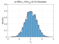
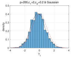
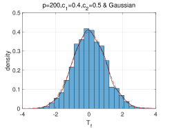
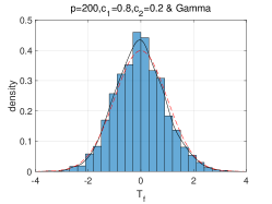
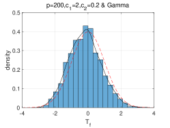
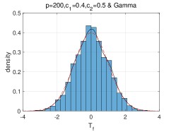
Figure 1: Empirical distribution of $T_{x,1}$ under the null in Model 2 when $M_{0}=6$ and $f(x)=x$.

Table 2: Empirical size of rejecting the null hypothesis (2.6) in Model 2, when the true value of $M$ is 6 and $f(x)=\log x$.

Values of $M_{0}$	$M_{0}=1$	$M_{0}=2$	$M_{0}=3$	$M_{0}=4$	$M_{0}=5$	$M_{0}=6$	$M_{0}=7$
Mode1 under Gaussian assumption
$p=100,c_{1}=0.05,c_{2}=0.5$	0.1040	0.5130	0.9940	0.9110	0.4735	0.0410	0.2195
$p=200,c_{1}=0.05,c_{2}=0.5$	0.1090	0.4980	0.9965	0.9045	0.4805	0.0475	0.2540
$p=400,c_{1}=0.05,c_{2}=0.5$	0.1175	0.4985	0.9940	0.9025	0.4825	0.0480	0.2545
$p=100,c_{1}=0.4,c_{2}=0.5$	0.0800	0.3325	0.9470	0.7290	0.3085	0.0340	0.1670
$p=200,c_{1}=0.4,c_{2}=0.5$	0.0825	0.3245	0.9475	0.7190	0.3035	0.0410	0.1695
$p=400,c_{1}=0.4,c_{2}=0.5$	0.0925	0.3305	0.9370	0.7250	0.3170	0.0480	0.2025
$p=100,c_{1}=0.5,c_{2}=0.05$	0.1070	0.4950	0.9945	0.9195	0.4900	0.0445	0.0980
$p=200,c_{1}=0.5,c_{2}=0.05$	0.1185	0.4915	0.9960	0.9035	0.4805	0.0405	0.0985
$p=400,c_{1}=0.5,c_{2}=0.05$	0.1115	0.4815	0.9975	0.9050	0.4905	0.0445	0.1160
Mode1 under Gamma assumption
$p=100,c_{1}=0.05,c_{2}=0.5$	0.0725	0.2715	0.8865	0.6175	0.2515	0.0370	0.1300
$p=200,c_{1}=0.05,c_{2}=0.5$	0.0800	0.2635	0.8765	0.6140	0.2565	0.0410	0.1340
$p=400,c_{1}=0.05,c_{2}=0.5$	0.0815	0.2685	0.8675	0.6160	0.2565	0.0465	0.1375
$p=100,c_{1}=0.4,c_{2}=0.5$	0.0605	0.1710	0.6985	0.4100	0.1545	0.0300	0.0780
$p=200,c_{1}=0.4,c_{2}=0.5$	0.0670	0.1720	0.6845	0.4230	0.1575	0.0445	0.1020
$p=400,c_{1}=0.4,c_{2}=0.5$	0.0635	0.1785	0.6985	0.4230	0.1690	0.0395	0.1095
$p=100,c_{1}=0.5,c_{2}=0.05$	0.0795	0.2555	0.8780	0.6165	0.2335	0.0385	0.0555
$p=200,c_{1}=0.5,c_{2}=0.05$	0.0810	0.2655	0.8775	0.6225	0.2535	0.0440	0.0710
$p=400,c_{1}=0.5,c_{2}=0.05$	0.0875	0.2650	0.8835	0.6195	0.2555	0.0470	0.0845

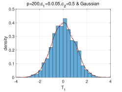
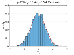
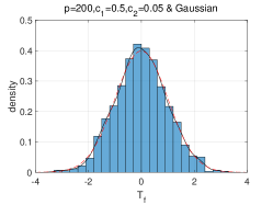
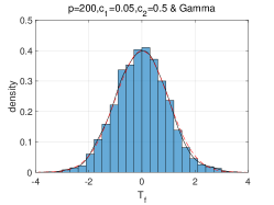
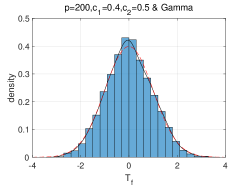
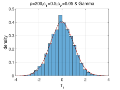
Figure 2: Empirical distribution of $T_{log,1}$ under the null in Model 2 when $M_{0}=6$ and $f(x)=\log x$.

3 Application to variable selection in a large-dimensional linear model

For multivariate linear models, Wilk’s likelihood ratio test (LRT) is one of the important analytical tools. In a high-dimensional setting, [3] developed a modified Wilk’s test based on RMT, whose test statistic is a function of the eigenvalues of a Fisher matrix. Their corrected LRT is asymptotically normal under the null. In this section, we modify the wilk’s $\Lambda_{n}$ from another perspective to test the number of significant variables, and the test statistic is in the form of a function of the eigenvalues of the spiked Fisher matrix.

3.1 Testing the number of significant variables

Consider a large-dimensional linear regression model, that is, the dimension and number of regression variables increase proportionally with the increase of the sample size. The independent observations $\left\{\mathbf{z}_{i}\right\}_{1\leqslant i\leqslant n}$ are $p$-dimensional from the following regression model

$$\mathbf{z}_{i}=\mathbf{B}\mathbf{w}_{i}+\bm{\epsilon}_{i},\quad i=1,\ldots,n,$$ (3.1)

where $\{\mathbf{w}_{i}\}_{1\leqslant i\leqslant n}$ are known design vectors (or regression variables) of dimensional $r$, $\mathbf{B}$ is a $p\times r$ matrix of regression coefficients, and $\{\bm{\epsilon}_{i}\}_{1\leqslant i\leqslant n}$ are a sequence of i.i.d. errors drawn from $\mathcal{N}_{p}(\mathbf{0},\mathbf{V})$. Assume that $n\geqslant p+r$ and the rank of $\mathbf{W}=\left(\mathbf{w}_{1},\mathbf{w}_{2},\cdots,\mathbf{w}_{n}\right)$ is $r$.

Partition the matrix $\mathbf{B}$ as $\left(\mathbf{B}_{1},\mathbf{B}_{2}\right)$ with $r_{1}$ and $r_{2}$ columns, respectively, satisfying $r_{1}+r_{2}=r$. To deal with large-dimensional data, it is assumed that $p/r_{1}\rightarrow y_{1}\in(0,\infty)$, $p/(n-r)\rightarrow y_{2}\in(0,1)$ as $\min(p,r_{1},n-r)\rightarrow\infty$. Assuming that $M_{0}$ is the true number of non-zero columns of $\mathbf{B}_{1}$, i.e. the true number of significant variables, consider the following hypothesis:

$$\mathcal{H}_{0}:M=M_{0}\quad v.s.\quad\mathcal{H}_{1}:M\neq M_{0}.$$ (3.2)

In particular, when $M_{0}=0$, the hypothesis (3.2) is equivalent to the hypothesis of $\mathcal{H}_{0}:\mathbf{B}_{1}=\mathbf{0}$ in [3]. That is, our hypothesis test is more general and can cover this hypothesis test.

The well-known Wilk’s statistic was originally proposed in [36, 37] and studied in [9]. Divide $\mathbf{w_{i}}^{T}$ into $\left(\mathbf{w}_{i,1}^{T},\mathbf{w}_{i,2}^{T}\right)$ in a same manner corresponding to the partition of $\mathbf{B}=\left(\mathbf{B}_{1},\mathbf{B}_{2}\right)$, then the Wilk’s LRT statistic can be defined as

$${\Lambda}_{n}=\frac{\left|\hat{\mathbf{V}}\right|}{\left|\hat{\mathbf{V}}_{0}\right|}=\frac{\left|1/n\sum_{i=1}^{n}\left(\mathbf{z}_{i}-\hat{\mathbf{B}}\mathbf{w}_{i}\right)\left(\mathbf{z}_{i}-\hat{\mathbf{B}}\mathbf{w}_{i}\right)^{T}\right|}{\left|1/n\sum_{i=1}^{n}\left(\mathbf{x}_{i}-\hat{\mathbf{B}}_{20}\mathbf{w}_{i,2}\right)\left(\mathbf{x}_{i}-\hat{\mathbf{B}}_{20}\mathbf{w}_{i,2}\right)^{T}\right|},$$ (3.3)

where $\hat{\mathbf{B}}=\left(\sum_{i=1}^{n}\mathbf{z}_{i}\mathbf{w}_{i}^{T}\right)\left(\sum_{i=1}^{n}\mathbf{w}_{i}\mathbf{w}_{i}^{T}\right)^{-1}$ is the maximum likelihood estimator of $\mathbf{B}$ in the full parameter space, $\hat{\mathbf{B}}_{20}=\sum_{i=1}^{n}\mathbf{x}_{i}\mathbf{w}_{i,2}^{T}\left(\sum_{i=1}^{n}\mathbf{w}_{i,2}\mathbf{w}_{i,2}^{T}\right)^{-1}$ is the maximum likelihood estimator of $\mathbf{B}_{2}$ under the null, and $\mathbf{x}_{i}=\mathbf{z}_{i}-\mathbf{B}_{1}\mathbf{w}_{i,1}$.

Define $\mathbf{A}_{11:2}=\sum_{i=1}^{n}\mathbf{w}_{i,1}\mathbf{w}_{i,1}^{T}-\sum_{i=1}^{n}\mathbf{w}_{i,1}\mathbf{w}_{i,2}^{T}\left(\sum_{i=1}^{n}\mathbf{w}_{i,2}\mathbf{w}_{i,2}^{T}\right)^{-1}\sum_{i=1}^{n}\mathbf{w}_{i,2}\mathbf{w}_{i,1}^{T}.$ By some calculations elaborated as in [1], the LRT $\Lambda_{n}$ defined in (3.3) can be re-expressed as

$${\Lambda}_{n}=\left|\mathbf{I}+\frac{r_{1}}{n-r}\mathbf{H}_{0}\mathbf{G}^{-1}\right|^{-1},$$ (3.4)

where $\mathbf{H}_{0}=(\hat{\mathbf{B}}_{1}-\mathbf{B}_{1})\mathbf{A}_{11:2}(\hat{\mathbf{B}}_{1}-\mathbf{B}_{1})^{T}/r_{1},\mathbf{G}=n\hat{\mathbf{V}}/(n-r),$ and $\hat{\mathbf{B}}_{1}$ consists of the first $r_{1}$ columns of $\hat{\mathbf{B}}$. Make a notation that $W_{p}(\cdot,\kappa)$ represents the $p$-dimensional Wishart distribution with $\kappa$ degrees of freedom. Under the null, according to [1], there are

$$(n-r)\mathbf{G}\sim W_{p}(\mathbf{V},n-r),\quad r_{1}\mathbf{H}_{0}\sim W_{p}(\mathbf{V},r_{1}),$$ (3.5)

and $\mathbf{H}_{0}$ is independent of $\mathbf{G}$. Thus $\mathbf{H}_{0}\mathbf{G}^{-1}$ is distributed as the Fisher matrix.

Now we modify the LRT statistic defined in (3.4) to test the number of significant variables. Define the corrected LRT as

$$\Lambda_{n}^{*}=\left|\mathbf{I}+\frac{r_{1}}{n-r}\mathbf{H}\mathbf{G}^{-1}\right|^{-1},$$ (3.6)

where

$$\mathbf{H}=\frac{\hat{\mathbf{B}}_{1}\mathbf{A}_{11:2}\hat{\mathbf{B}}_{1}^{T}}{r_{1}}$$

is independent of $\mathbf{G}$. The matrix $\mathbf{H}$ can be decomposed as

$$\mathbf{H}=\mathbf{H}_{0}+\mathbf{\Delta}_{0},$$

where $\mathbf{\Delta}_{0}=(\hat{\mathbf{B}}_{1}\mathbf{A}_{11:2}\mathbf{B}_{1}^{T}+\mathbf{B}_{1}\mathbf{A}_{11:2}\hat{\mathbf{B}}_{1}^{T}-\mathbf{B}_{1}\mathbf{A}_{11:2}\mathbf{B}_{1}^{T})/r_{1}$, has $M_{0}$ dominated eigenvalues. Then $r_{1}\mathbf{H}$ is a perturbation of rank $M_{0}$ on the matrix $r_{1}\mathbf{H}_{0}$ that follows $W_{p}(\mathbf{V},r_{1})$. We illustrate the properties of the eigenvalues of $\mathbf{H}$ with an example in the Appendix A.5.

Combining the formula (3.5), under the null in (3.2), the matrix $\mathbf{H}\mathbf{G}^{-1}$ is exactly distributed as the spiked Fisher matrix defined in (2.2) with $M_{0}$ spikes. Consequently, we can use this matrix to test the number of of spikes, which is equivalent to test the number of significant regression variables. Denote the eigenvalues of $\mathbf{H}\mathbf{G}^{-1}$ in the descending order as below:

$$\ell_{1}\ \geqslant\ \ell_{2}\ \geqslant\ \cdots\geqslant\ \cdots\ \geqslant\ \ell_{p}.$$

The largest $M_{0}$ eigenvalues are sample spiked eigenvalues. Then the test statistic for $\eqref{H2}$ can be constructed in the form of a partial eigenvalue function defined in (2.7) as

$$-\log{\Lambda}_{n}^{*}-\sum_{i=1}^{M}\log(1+\frac{y_{2}}{y_{1}}\ell_{i}).$$

Its CLT is established as follows.

Theorem 3.1.

For the testing problem (3.2) in the large-dimensional linear regression model (3.1), define $\Lambda_{n}^{*}$ as in the formula (3.6), and assuming that $p/r_{1}\rightarrow y_{1}\in(0,\infty)$, $p/(n-r)\rightarrow y_{2}\in(0,1)$ as $\min(p,r_{1},n-r)\rightarrow\infty$. Then under the null, we have

$$T_{l} =v_{l}^{-\frac{1}{2}}\left[-\log{\Lambda}_{n}^{*}-\sum_{i=1}^{M}\log(1+\frac{y_{2}}{y_{1}}\ell_{i})-d_{l}+\sum\limits_{i=1}^{M}\log(1+\frac{y_{2}}{y_{1}}\psi_{i})-u_{l}\right]$$

$$\Rightarrow\mathcal{N}(0,1),$$ (3.7)

where

$$d_{l}=p\int\log(1+\frac{y_{2}}{y_{1}}x)dF^{(c_{n1},c_{n2},H_{n})}(x)$$

can be obtained by Algorithm 1, and

$$\mu_{l}=\frac{1}{2}\log\frac{\left(c^{2}-d^{2}\right)h^{2}}{\left(ch-c_{2}d\right)^{2}},\quad\nu_{l}=2\log\left(\frac{c^{2}}{c^{2}-d^{2}}\right).$$

Here

$$h =\sqrt{y_{1}+y_{2}-y_{1}y_{2}},$$

$$a,b =\frac{\left(1\mp h\right)^{2}}{\left(1-y_{2}\right)^{2}},\quad a<b,$$

$$c,d =\frac{1}{2}\left(\sqrt{1+\frac{y_{2}}{y_{1}}b}\pm\sqrt{1+\frac{y_{2}}{y_{1}}a}\right),\quad c>d.$$

3.2 Simulation study

In this section, Monte Carlo simulations are conducted to illustrate the performance of our proposed test statistics for the hypothesis (3.2). We first generate data from the following model:

$$\mathbf{z}_{i}=\mathbf{B}\mathbf{w}_{i}+\bm{\epsilon}_{i},\quad i=1,\ldots,n,$$

where the entries of regression variables $\mathbf{w}_{i}$ are i.i.d. drawn from $\mathcal{N}(0,1)$, the regression coefficient matrix $\mathbf{B}$ is decomposed into $(\mathbf{B}_{1},\mathbf{B}_{2})$, $\mathbf{B}_{1}=(\mathbf{b}_{1},\mathbf{b}_{2},\mathbf{b}_{3},\mathbf{b}_{4},\\ \mathbf{b}_{5},\mathbf{0},\mathbf{0},\cdots,\mathbf{0})$ with the entries of $\mathbf{b}_{i}(i=1,2,\cdots,5)$ being i.i.d. from $\mathcal{N}(0,1)$, $\mathbf{B}_{2}=\mathbf{0}$. Thus $M_{0}=5$. The error $\bm{\epsilon}_{i}$ is a $p\times 1$ vector drawn from $\mathcal{N}_{p}(0,\mathbf{V})$, where the population covariance matrix $\mathbf{V}$ is considered as the following three models.

Model 3. Assuming that the matrix $\mathbf{V}$ is an identity matrix.

Model 4. Assuming that the matrix $\mathbf{V}$ is in the form of a Toeplitz matrix defined as

$$\mathbf{V}=\left(\begin{array}[]{ccccc}1&\rho&\rho^{2}&\cdots&\rho^{p-1}\\ \rho&1&\rho&\cdots&\rho^{p-2}\\ \cdots&\cdots&&&\\ \rho^{p-1}&\rho^{p-2}&\cdots&\rho&1\end{array}\right),$$

where $\rho=0.9$.

Model 5. Assuming that the matrix $\mathbf{V}=\mathbf{U_{0}\Lambda U_{0}^{*}}$, where

$$\mathbf{\Lambda}= \text{diag}(\underbrace{0.2,\cdots,0.2}_{p/5},\underbrace{0.4,\cdots,0.4}_{p/5},\underbrace{0.6,\cdots,0.6}_{p/5},\underbrace{0.8,\cdots,0.8}_{p/5},\underbrace{1,\cdots,1}_{p/5}),$$

$\mathbf{U}_{0}$ is composed of the eigenvectors of a $p\times p$ matrix $\mathbf{D}\mathbf{D}^{*}$ with the entries of $\mathbf{D}$ being independently sampled from $\mathcal{N}(0,1)$.

For each scenario, the value of $y_{1}$ is set to $0.5,1.5$, and $y_{2}$ is set to $0.2,0.5,0.8$. Reported in Table 3 to 4 are the empirical sizes and powers of our proposed test statistics $T_{l}$ in (3.1) rejecting the null with 2,000 replications at a significance level $\alpha=0.05$, for Model 4 and Model 5, respectively. The simulation results of Model 3 are presented in the supplementary material for space.

As shown in the tables, the empirical sizes of our proposed test can achieve correct empirical sizes around 0.05 for all models. When the distance between the alternative hypothesis and the null hypothesis is larger, the higher the power is. Figure 3 and 4 depict the simulated empirical distributions of our proposed test statistic in several cases from Model 4 and Model 5, when the null hypothesis is true. We can find that the empirical distribution of the statistic fits well with the standard normal distribution. Moreover, note that $\rho$ defined in Model 4 denotes the degree of correlation between $p$ components of error vectors. Model 3 is the case of $\rho=0$. Model 3 and 4 represent that the errors are completely uncorrelated or strongly correlated. The results indicate that our test method can provide good sizes, regardless of the correlations among the coordinates of the error vectors. In summary, it is proved that our proposed test method can accurately determine the number of significant variables in different scenarios.

Table 3: Empirical size of rejecting the null in Model 4.

Values of $M_{0}$	$M_{0}=1$	$M_{0}=2$	$M_{0}=3$	$M_{0}=4$	$M_{0}=5$	$M_{0}=6$
$p=40,n=300,r=100,r_{1}=80$	1	1	1	1	0.0340	0.7410
$p=80,n=600,r=200,r_{1}=160$	1	1	1	1	0.0440	0.7890
$p=160,n=1200,r=400,r_{1}=320$	1	1	1	1	0.0465	0.7925
$p=50,n=300,r=200,r_{1}=100$	1	1	1	1	0.0380	0.7890
$p=100,n=600,r=400,r_{1}=200$	1	1	1	1	0.0425	0.8040
$p=200,n=1200,r=800,r_{1}=400$	1	1	1	1	0.0550	0.814
$p=80,n=300,r=200,r_{1}=160$	1	1	1	0.9995	0.0360	0.8315
$p=160,n=600,r=400,r_{1}=320$	1	1	1	1	0.0415	0.8515
$p=320,n=1200,r=800,r_{1}=640$	1	1	1	1	0.0520	0.8500
$p=60,n=350,r=50,r_{1}=40$	1	1	1	1	0.0310	0.7040
$p=120,n=700,r=100,r_{1}=80$	1	1	1	1	0.0440	0.7525
$p=240,n=1400,r=200,r_{1}=160$	1	1	1	1	0.0450	0.7825
$p=90,n=350,r=170,r_{1}=60$	1	1	1	1	0.0345	0.7525
$p=180,n=700,r=340,r_{1}=120$	1	1	1	1	0.0345	0.7770
$p=360,n=1400,r=680,r_{1}=240$	1	1	1	1	0.0475	0.7920
$p=120,n=350,r=200,r_{1}=80$	1	1	1	1	0.0340	0.7980
$p=240,n=700,r=400,r_{1}=160$	1	1	1	1	0.0410	0.8130
$p=480,n=1400,r=800,r_{1}=320$	1	1	1	1	0.0445	0.8355

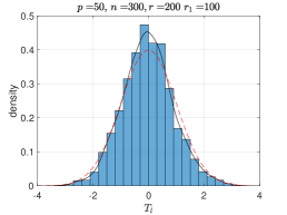
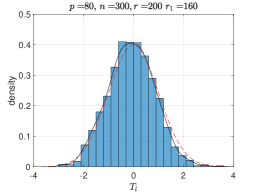
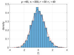
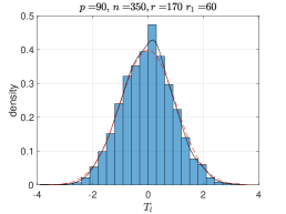
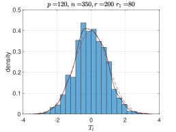
Figure 3: Empirical distribution of $T_{l}$ under the null in Model 4

Table 4: Empirical size of rejecting the null in Model 5

Values of $M_{0}$	$M_{0}=1$	$M_{0}=2$	$M_{0}=3$	$M_{0}=4$	$M_{0}=5$	$M_{0}=6$
$p=40,n=300,r=100,r_{1}=80$	1	1	1	1	0.0365	0.7615
$p=80,n=600,r=200,r_{1}=160$	1	1	1	1	0.0380	0.7845
$p=160,n=1200,r=400,r_{1}=320$	1	1	1	1	0.0410	0.8050
$p=50,n=300,r=200,r_{1}=100$	1	1	1	1	0.0365	0.7705
$p=100,n=600,r=400,r_{1}=200$	1	1	1	1	0.0410	0.7920
$p=200,n=1200,r=800,r_{1}=400$	1	1	1	1	0.0500	0.8155
$p=80,n=300,r=200,r_{1}=160$	1	1	1	0.9940	0.0420	0.8260
$p=160,n=600,r=400,r_{1}=320$	1	1	1	0.9990	0.0450	0.8480
$p=320,n=1200,r=800,r_{1}=640$	1	1	1	0.9995	0.0465	0.8520
$p=60,n=350,r=50,r_{1}=40$	1	1	1	1	0.0360	0.6890
$p=120,n=700,r=100,r_{1}=80$	1	1	1	1	0.0385	0.7485
$p=240,n=1400,r=200,r_{1}=160$	1	1	1	1	0.0475	0.7655
$p=90,n=350,r=170,r_{1}=60$	1	1	1	1	0.0345	0.7515
$p=180,n=700,r=340,r_{1}=120$	1	1	1	1	0.0380	0.7885
$p=360,n=1400,r=680,r_{1}=240$	1	1	1	1	0.0480	0.8015
$p=120,n=350,r=200,r_{1}=80$	1	1	1	1	0.0365	0.8090
$p=240,n=700,r=400,r_{1}=160$	1	1	1	1	0.0425	0.8235
$p=480,n=1400,r=800,r_{1}=320$	1	1	1	1	0.470	0.8460

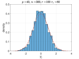
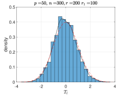
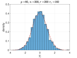
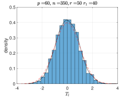
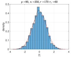
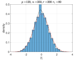
Figure 4: Empirical distribution of $T_{l}$ under the null in Model 5

4 Application to detecting the change points

Change point detection can identify mutations of some statistical characteristics in sequence data. As a processing tool, it has proven useful in many applications such as electroencephalogram analysis, DNA segmentation, econometrics, and disease demography, etc.

Among some existing methods for change point detection, sliding time window is one of the basic tools. Referred to [22], cut the samples within the time window $W_{j},j=1,2,\cdots$ into two groups, and the corresponding population covariance matrices are denoted as $\mathbf{\Sigma}_{j}^{(1)}$ and $\mathbf{\Sigma}_{j}^{(2)}$ respectively. Then the equality of these two populations can be determined by checking whether the Fisher matrix $\mathbf{F}_{j}=(\bm{\Sigma}_{j}^{(1)})^{-1}\bm{\Sigma}_{j}^{(2)}$ is equal to an identity matrix $\mathbf{I}$. When there are no anomalies in $W_{j}$, we have $\mathbf{F}_{j}=\mathbf{I}$, which is equivalent to the number of spikes in $\mathbf{F}$ being 0. In contrast, when anomalies are introduced in $W_{j}$, the number of spikes in $\mathbf{F}_{j}$ is not equal to 0. This is the heart of the change point detection method proposed in this section.

4.1 Change point detection

Consider a $p$-dimensional time series data $\mathbf{X}=\left(\mathbf{x}_{1},\mathbf{x}_{2},\cdots,\mathbf{x}_{T}\right)$ of length $T$ with both change points and additive outliers, and the locations of which are unknown in practice. Additive outliers affect only the single observation to which they are attached, while change points occur in a relatively long period of time. Assume that the change points occur at time $t_{c}$. Now we want to design a method to correctly detect the location of $t_{c}$ with avoiding the influence of additive outliers.

Our change point detection method is constructed based on the point-by-point sliding time window. Each time sliding, the sample at the front of the window will be removed, and a new sample will be added at the end of the window. Here an empty set $\mathcal{T}$ is created for subsequent use. Suppose the width of the first window $W_{1}$ is $q_{1}$, divide the data in $W_{1}$ into two groups with length $q_{11}$ and $q_{12}$, denoted as $\mathbf{X}_{1}^{(1)}=(\mathbf{x}_{1},\mathbf{x}_{2},\cdots,\mathbf{x}_{q_{11}})$ and $\mathbf{X}_{1}^{(2)}=(\mathbf{x}_{q_{11}+1},\mathbf{x}_{q_{11}+2},\cdots,\mathbf{x}_{q_{11}+q_{12}})$, satisfying $q_{1}=q_{11}+q_{12}$. Further denote the population covariance matrices of $\mathbf{X}_{1}^{(1)}$ and $\mathbf{X}_{1}^{(2)}$ as $\bm{\Sigma}_{1}^{(1)}$ and $\bm{\Sigma}_{1}^{(2)}$, respectively. Consider the following hypothesis

$$\mathcal{H}_{0}:(\bm{\Sigma}_{1}^{(1)})^{-1}\bm{\Sigma}_{1}^{(2)}=\mathbf{I}\quad v.s.\quad\mathcal{H}_{1}:(\bm{\Sigma}_{1}^{(1)})^{-1}\bm{\Sigma}_{1}^{(2)}\neq\mathbf{I}.$$ (4.1)

If the null hypothesis in (4.1) holds, it indicates that there are no abnormal points in $\mathbf{W}_{1}$, and then continue to slide a point to the next window. Keep sliding by this way until the null hypothesis does not holds within a certain window $W_{j}$. To be specific, let the two groups of samples in $W_{j}$ be

$$\mathbf{X}_{j}^{(1)} =(\mathbf{x}_{j+1},\mathbf{x}_{j+2},\cdots,\mathbf{x}_{j+q_{j1}}),$$

$$\mathbf{X}_{j}^{(2)} =(\mathbf{x}_{j+q_{j1}+1},\mathbf{x}_{j+q_{j1}+2},\cdots,\mathbf{x}_{j+q_{j1}+q_{j2}}),$$ (4.2)

from two populations $\bm{\Sigma}_{j}^{(1)}$ and $\bm{\Sigma}_{j}^{(2)}$ with lengths $q_{j1}={q_{11}}$ and $q_{j2}={q_{12}}$. The null hypothesis in

$$\mathcal{H}_{0}:(\bm{\Sigma}_{j}^{(1)})^{-1}\bm{\Sigma}_{j}^{(2)}=\mathbf{I}\ v.s.\ \mathcal{H}_{1}:(\bm{\Sigma}_{j}^{(1)})^{-1}\bm{\Sigma}_{j}^{(2)}\neq\mathbf{I},\ j=2,3,\cdots$$ (4.3)

doesn’t holds, which means that the newly added sample $\mathbf{x}_{j+q_{j1}+q_{j2}}$ in $W_{j}$ is abnormal. Then delete the abnormal point $\mathbf{x}_{j+q_{j1}+q_{j2}}$, and add the location $j+q_{j1}+q_{j2}$ to the set $\mathcal{T}$. Fix the length of the first group of samples in all windows to $q_{11}$, then the two groups of data with lengths $q_{j+1,1}$ and $q_{j+1,2}$ in the window $W_{j+1}$ become

$$\mathbf{X}_{j+1}^{(1)} =(\mathbf{x}_{j+2},\mathbf{x}_{j+3},\cdots,\mathbf{x}_{j+q_{j1}+1}),$$

$$\mathbf{X}_{j+1}^{(2)} =(\mathbf{x}_{j+q_{j1}+2},\mathbf{x}_{j+q_{j1}+2},\cdots,\mathbf{x}_{j-1+q_{j1}+q_{j2}},\mathbf{x}_{j+1+q_{j1}+q_{j2}}),$$ (4.4)

which satisfy $q_{j+1,1}=q_{j1}=q_{11}$ and $q_{j+1,2}=q_{j2}-1=q_{12}-1$. It can be concluded that the change point in the data has been detected when abnormal points are detected in $s$ consecutive windows, i.e., $s$ consecutive numbers appear in the set of $\mathcal{T}$. The first value of the $s$ consecutive numbers is determined as the location $t_{c}$ where the change point occurs. By the removal of abnormal points, for the lengths of two groups of data in all windows, we have $q_{11}=q_{21}=\cdots=q_{j1}=\cdots$, and $q_{12}\geq q_{22}\geq\cdots\geq q_{j2}\geq\cdots$.

It should be noted that the operation of deleting abnormal samples from (4.1) to (4.1) is a critical step to avoid the influence of additive outliers on change point detection. If deletion is not performed, the newly introduced additive outliers will exist in multiple consecutive time windows until they slip out of the window, which can also produce consecutive $s$ anomalous results and thus lead to incorrect change point location detection.

Assuming that the number of spikes of the Fisher matrix $(\bm{\Sigma}_{j}^{(1)})^{-1}\bm{\Sigma}_{j}^{(2)}$ in the window $W_{j}$ is $M_{j}$, $j=1,2,\cdots$, then the hypotheses (4.1) and (4.3) are equivalent to the following one

$$\mathcal{H}_{0}:M_{j}=0\quad v.s.\quad\mathcal{H}_{1}:M_{j}\neq 0,j=1,2,\cdots.$$ (4.5)

This is a degenerate test for testing the non-zero number of spikes.

Let the unbiased sample covariance matrices corresponding to the data $\mathbf{X}_{j}^{(1)}$ and $\mathbf{X}_{j}^{(2)}$ in the window $W_{j}$ be $\mathbf{S}_{j}^{(1)}$ and $\mathbf{S}_{j}^{(2)}$. Then for the hypothesis (4.5), we use $\mathrm{tr}[(\mathbf{S}_{j}^{(1)})^{-1}\mathbf{S}_{j}^{(2)}]$ as the test statistic. We normalize the first group of data $\mathbf{X}_{j}^{(1)}$ as $\bm{\xi}_{j}^{(1)}$, and $\mathbf{X}_{j}^{(2)}$ as $\bm{\xi}_{j}^{(2)}$. Further define $\phi_{j}^{(1)}=E\left|\xi_{j,11}^{(1)}\right|^{4}$, $\phi_{j}^{(2)}=E\left|\xi_{j,11}^{(2)}\right|^{4}$, where $\xi_{j,11}^{(1)}$ and $\xi_{j,11}^{(2)}$ are the $(1,1)$-th entries of the matrices $\mathbf{X}_{j}^{(1)}$ and $\mathbf{X}_{j}^{(2)}$, respectively. Then the asymptotic distribution of the test statistic is established as follows.

Theorem 4.1.

For the testing problem (4.3) in each window $W_{j},j=1,2,\cdots$, assuming that $p/q_{j1}\rightarrow y_{j}^{(1)}\in(0,1)$, $p/q_{j2}\rightarrow y_{j}^{(2)}\in(0,+\infty)$ as $\min(p,q_{j1},q_{j2})\rightarrow\infty$. Then under the null, we have

$$T_{j}=\nu_{x}^{-\frac{1}{2}}\left\{\mathrm{tr}[(\mathbf{S}_{j}^{(1)})^{-1}\mathbf{S}_{j}^{(2)}]-d_{x}-\mu_{x}\right\}\Rightarrow\mathcal{N}(0,1),$$ (4.6)

where

$$d_{x} =\frac{p}{1-y_{j}^{(1)}},$$

$$\mu_{x,1} =\frac{qy_{j}^{(1)}}{(1-y_{j}^{(1)})^{2}}+\frac{\beta_{j}^{(1)}y_{j}^{(1)}}{1-y_{j}^{(1)}},$$

$$\nu_{x} =\frac{(q+1)h_{j}^{2}}{(1-y_{j}^{(1)})^{4}}+\frac{\beta_{j}^{(1)}y_{j}^{(1)}+\beta_{j}^{(2)}y_{j}^{(2)}}{(1-y_{j}^{(1)})^{2}}.$$

Here $h_{j}^{2}=(y_{j}^{(1)})^{2}+(y_{j}^{(2)})^{2}-y_{j}^{(1)}y_{j}^{(2)}$, $\beta_{j}^{(1)}={\phi_{j}^{(1)}-q-2}$ and $\beta_{j}^{(2)}={\phi_{j}^{(2)}-q-2}$ with $q=1$ for real case and $q=0$ for complex.

With the CLT in Theorem 4.1, we reorganize the steps to detect the change point as the following Algorithm 2 .

Algorithm 2 Change point detection Based on Hypothesis Testing.

0:  $\mathbf{X}=\left(\mathbf{x}_{1},\mathbf{x}_{2},\cdots,\mathbf{x}_{T}\right)$; $q_{11},q_{12}$; $s$; an empty set $\mathcal{T}$.

0:  The location $t_{c}$ of change point.

1:  $j=0$;

2:  while There are no $s$ consecutive numbers in the set $\mathcal{T}$ do

3:     $j=j+1$;

4:     Calculate $T_{j}$ in the window $W_{j}$ according to (4.6);

5:     if $T_{j}$ falls outside the rejection region then

6:        Slide the Window to $W_{j+1}$;

7:     else

8:        Delete the sample $x_{t_{0}}$ at the end of $W_{j}$, where $t_{0}$ is the location of this sample in the data $\mathbf{X}$ ;

9:        Add $t_{0}$ to the set $\mathcal{T}$;

10:        Slide the Window to $W_{j+1}$;

11:     end if

12:  end while

13:  Obtain the first value of the $s$ consecutive numbers in $\mathcal{T}$ as the location $t_{c}$ where the change point occurs.

4.2 Simulation study

In this section, extensive simulation studies are conducted to compare our proposed change-point detection method with three other methods in the existing literature. In the presentation of the simulation results below, we label the following three methods as M-P, MSR, and SVM.

• M-P: [32] finds the change point by judging whether the largest eigenvalue of the sample covariance matrix is located outside the support set of the standard Marčenko-Pastur law .

• MSR: [41] detects the change point by judging whether the mean spectral radius (MSR) calculated from the sample data is smaller than the inner ring radius of the single ring law.

• SVM: With the classifications of normal data and abnormal data, [19] use training data to obtain Support Vector Machines (SVM) model, and predict whether there is abnormality in test data.

We consider the following three models.

Model 6. $\mathbf{x}_{t}\stackrel{{\scriptstyle\text{ i.i.d. }}}{{\sim}}N(\mu,\mathbf{I}_{p})$ for $1\leq t\leq\lfloor 2/3T\rfloor$, $\mathbf{x}_{t}\stackrel{{\scriptstyle\text{ i.i.d. }}}{{\sim}}N(\mu,\rho_{1}\mathbf{I}_{p})$ for $\lfloor 2/3T\rfloor+1\leq t\leq T$, where $\mu=(0.6,\ldots,0.6)\in\mathbb{R}^{p}$.

Model 7. ${x}_{t,k}\stackrel{{\scriptstyle i.i.d.}}{{\sim}}$ Poisson(1) for $k=1,\ldots,p$ and $1\leq t\leq\lfloor 2/3T\rfloor$, $x_{t,k}\stackrel{{\scriptstyle i.i.d.}}{{\sim}}$ Exponential ($\rho_{2}$) for $k=1,\ldots,p$ and $\lfloor 2/3T\rfloor+1\leq t\leq T$.

Model 8. $\mathbf{x}_{t}=\mathbf{A}\mathbf{F}_{t}+\mathbf{e}_{t}$, where $\mathbf{A}$ is a $p\times 5$ factor loading matrix with each element generated from a uniform distribution $U(0.5,1.5)$, the factors $\mathbf{F}_{t}\stackrel{{\scriptstyle\text{ i.i.d. }}}{{\sim}}N(\mathbf{0}_{5},\mathbf{I}_{5})$ and the error terms $\mathbf{e}_{t}\stackrel{{\scriptstyle\text{ i.i.d. }}}{{\sim}}N(0_{p},\mathbf{\Sigma}_{e})$. $\mathbf{\Sigma}_{e}=I_{p}$ for $1\leq t\leq\lfloor 2/3T\rfloor$, $\mathbf{\Sigma}_{e}=(\sigma_{ij})_{i,j=1}^{p}$ with $\sigma_{ij}=\rho_{3}0.8^{|i-j|}$ for $\lfloor 2/3T\rfloor+1\leq t\leq T$.

The length of all generated data is $T=6000$. Within 6000 observations in the all three models, two additive outliers have been added at $t=2001,2002$, and the value is $20(\mathbf{1}_{p},\mathbf{1}_{p})$. Moreover, note that each of the above three models involves a parameter $\rho_{1}$, $\rho_{2}$ and $\rho_{3}$, respectively, which can reflect the magnitude of the change in distribution characteristics in the corresponding model. Specifically, in Model 6, the larger the $\rho_{1}$, the larger the difference between the covariance matrices after the time $2/3T$ and before $2/3T$. We set $\rho_{1}=5,10,20$ in Model 6, $\rho_{2}=2,4,8$ in Model 7, $\rho_{4}=3,6,9$ in Model 8, respectively. 100 pieces of simulated data are generated, $s$ takes the value of 20, $q_{11}=2p$ and $q_{12}=2p$. We define accuracy as the percentage of correctly detected change points in 100 pieces of data, which is used to be the indicator to reflect the detection performance of different methods.

First, since our proposed change point detection method requires multiple tests, the number of falsely rejecting the null hypothesis increases greatly as the number of tests increases. A commonly used method to adjust for multiplicity is the Bonferroni correction ([10]), where the significance level is set to $\alpha/n$ and $n$ is the number of tests. However, this method is too stringent. Here we adopt a compromise approach by using a numerical method to select a relatively low significance level $\alpha$. Set $\alpha$ to six values from large to small: 0.05, 0.01, 0.005, 0.001, 0.0005 and 0.0001, and we need to select one among them as the significance level for the test. For the above three models when $p=50$, with 100 replications, we obtain the accuracy under different values of $\alpha$, denoted as ${A_{i,j},i=1,2,3,j=1,2,\cdots,6}$. We regard the value that achieve an accuracy of about 95% as an ideal $\alpha$. Define the absolute errors between $A_{j}$ and $95\%$ as $e_{i,j}=|A_{i,j}-95\%|$. The absolute errors under different $\alpha$ in three models are shown in Figure 5. We use indexes 1, 2, 3, 4, 5 and 6 to represent significance levels 0.05, 0.01, 0.005, 0.001, 0.0005 and 0.0001, respectively. It can be observed that when $\alpha$ is taken as 0.0005, the absolute errors of all three models can reach a minimum value. Thus, $\alpha=0.0005$ is selected as the significance level for next simulations.

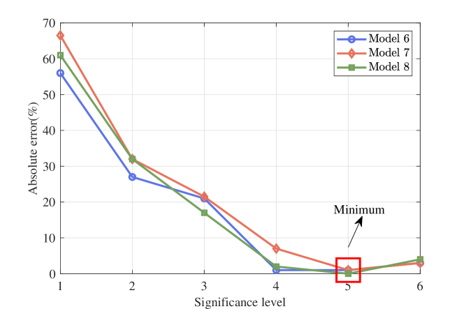
Figure 5: Absolute errors under different significant levels. Indexes 1, 2, 3, 4, 5 and 6 refer to significance levels 0.05, 0.01, 0.005, 0.001, 0.0005 and 0.0001, respectively.

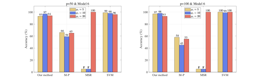
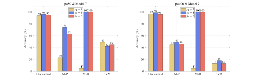
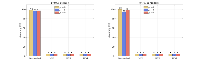
Figure 6: Accuracy comparisons among different methods in Model 6-8.

We set the dimension $p$ to 50 and 100 of each of the above Models, for each of which we compute the accuracy values and report them in Figure 6. Overall, it is evident that our proposed method outperforms the other three. Under the different cases, the detection accuracy of our proposed test method is as high as 95%. Moreover, M-P method has the obvious lowest detection accuracy in all three models. MSR method only performs well when the fluctuation of the change is large, but fails when the change fluctuates little, such as failing when $\rho_{1}=5$, $\rho_{1}=10$ in Model 6 and $\rho_{2}=2$ in Model 7. SVM method has high requirements for the structure of the training data. When we apply SVM method to the real data, it is difficult to know the specific model that the data comes from. So to fit the realistic scenario, we use the data generated by Model 6 as training data to obtain the SVM model for all three models. The results show that SVM method only has high prediction accuracy in model 6, but poor accuracy in the other two models, which means that the generalization performance of SVM method is poor. Besides, in the factor model setting of Model 8, both the M-P method and the MSR method also fail, which implies that these two methods are not suitable for data with spiked structure. Whereas our method achieves high detection accuracy in all cases across different models.

5 Real data

In this section, we demonstrate the performance of our proposed test method through an analysis of a public dataset of Africa Development Indicators, which is download from https://databank.worldbank.org/source/africa-development-indi
cators#. Africa Development Indicators data provides a detailed description of development in Africa. It contains macroeconomic, sectoral and social indicators, covering 53 African countries, with more than 1700 indicators from 1960 to 2011. The data collection is intended to provide all those interested in Africa with a quick reference and a reliable set of data to monitor development plans and aid flows in the region, which can be used to better understand the economic and social developments taking place in Africa.

We focus on development indicators of two countries in Africa, Kenya and South Africa. There are some null values in the dataset. We keep only the indicators with complete information and finally obtain the data for 40 development indicators from 1961 to 2010, i.e., $p=40,n_{1}=50,n_{2}=50$. Denote the population covariance matrices corresponding to the data of Kenyan and South Africa as $\mathbf{\Sigma}_{K}$ and $\mathbf{\Sigma}_{SA}$ respectively. And the associated sample covariance matrices are denoted as $\mathbf{S}_{K}$ and $\mathbf{S}_{SA}$. The Fisher matrix is constructed as $\mathbf{F}=\mathbf{S}_{K}\mathbf{S}_{SA}^{-1}$, and the number of spikes of this matrix is denoted as $M$. We want to test whether $\mathbf{\Sigma}_{K}$ and $\mathbf{\Sigma}_{SA}$ are equal, which is equivalent to consider the following hypothesis

$$\mathcal{H}_{0}:M=0\quad v.s.\quad\mathcal{H}_{1}:M\neq 0,$$

We use the test statistic $\operatorname{tr}({\bf F})$ for the above hypothesis and set the significance level of the test at 0.05, where $\operatorname{tr}(\cdot)$ denotes the trace of a matrix . We substitute $M_{0}=0$ and $f(x)=x$ into the CLT in Theorem 2.1, which is exactly the result in Example 2.1 when $M_{0}=0$. By applying the data,we find that the statistic falls in the rejection region under the null hypothesis. It implies that the number of spikes of $\mathbf{F}$ is not 0, that is, the two population covariance matrices are not equal. We apply the corrected LRT statistic in [43] to this data set to test the equality of the two populations, the results still indicates that the statistic falls in the rejection region, which is consistent with our results.

6 Conclusion

This paper discussed the problems of testing the number of spikes in a generalized two-sample spiked model. We proposed a universal test on this testing hypothesis problem, considered the partial linear spectra statistic as the test statistic and established its CLT under the null hypothesis. The theoretical results of our test method were applied to two problems in the high-dimensional settings, large dimensional linear regression and change point detection. We demonstrate the effectiveness of these tests and algorithms through extensive simulation studies and empirical study. Being independent of the population distribution and diagonal or block-wise assumption of the population covariance matrix, our proposed method have superior performance. The problem about testing the spikes in a non-central spiked Fisher matrix is also important, and thus warrants further research.

In addition, there is another issue that needs to be further studied. In section 3, our CLT in (3.1) is established under the normal population assumption of the error so as to obtain the conclusion that the matrices $\mathbf{G}$ and $\mathbf{H}_{0}$ follow Wishart distribution. However, it is experimentally verified that the CLT still holds when the population distribution of the error is non-normal, and some simulated results are put in the supplement material. The theoretical support of this result is not yet clear and still remains to be explored.

Appendix A Derivations and Proofs

A.1 Proof of Theorem 2.1

Proof.

We need to prove the CLT of the following partial linear spectral statistic

$$T=\sum\limits_{j=1}^{p}f\{l_{j}({\bf F})\}-\sum\limits_{j\in{\mathcal{J}}_{k},k=1}^{K}f\{l_{j}({\bf F})\}.$$ (A.1)

We first focus on the calculation of the second term $\sum\limits_{j\in{\mathcal{J}}_{k},k=1}^{K}f\{l_{j}({\bf F})\}$ in (A.1). It is known that, for the spiked sample eigenvalues of $\mathbf{F}$, almost surely,

$$\sum_{j\in\mathcal{J}_{k},k=1}^{K}f\{l_{j}({\bf F})\}\rightarrow\sum_{k=1}^{K}m_{k}f\left(\psi_{k}\right),$$ (A.2)

where $\psi_{k}$ is defined in (2.4).

For the first term in (A.1), we have

$$\sum\limits_{j=1}^{p}f\{l_{j}({\bf F})\} =p\int f(x)\mathrm{d}F_{\mathbf{n}}(x)$$

$$=p\int f(x)\mathrm{d}\left[F_{\mathbf{n}}(x)-F^{(c_{n1},c_{n2},H_{n})}(x)\right]+p\int f(x)\mathrm{d}F^{(c_{n1},c_{n2},H_{n})}(x),$$

where $F_{\mathbf{n}}$ is the empirical spectral distribution of the Fisher matrix ${\bf F}$, $F^{(c_{n1},c_{n2},H_{n})}$ is the distribution function in which the parameter $(c_{1},c_{2},H)$ is replaced by $(c_{n1},c_{n2},H_{n})$ in the LSD of ${\bf F}$.

We consider the following centered and scaled variables

$$p\int f(x)\mathrm{d}\left[F_{\mathbf{n}}(x)-F^{(c_{n1},c_{n2},H_{n})}(x)\right]=:G_{n}(x).$$

Therefore, we have

$$G_{n}(x)=\sum\limits_{j=1}^{p}f\{l_{j}({\bf F})\}-p\int f(x)\mathrm{d}F^{(c_{n1},c_{n2},H_{n})}(x).$$

Under different population assumptions, both of [42] and [44] proved that the process $G_{n}(x)$ would converge weakly to a Gaussian vector with explicit expressions of means and covariance functions when the dimensions are proportionally large compared to the sample sizes. The arrays of two random vectors in the Fisher matrix considered by [42] can be independent but differently distributed. [44] considered general Fisher matrices with arbitrary population covariance matrices, their proposed CLT extended and covered the conclusion of [42], and can be expressed as follows

$$G_{n}(x)\Rightarrow\mathcal{N}\left(\mu_{f},\quad\nu_{f}\right),$$

where

$$\mu_{f}= \frac{q}{4\pi i}\oint f(z){\rm d}\log\bigg{[}\frac{h^{2}}{c_{2}}-\frac{c_{1}}{c_{2}}\cdot\frac{\big{\{}1-c_{2}\int\frac{m_{0}(z)}{t+m_{0}(z)}{\rm d}H(t)\big{\}}^{2}}{1-c_{2}\int\frac{m^{2}_{0}(z)}{\big{\{}t+m_{0}(z)\big{\}}^{2}}{\rm d}H(t)}\bigg{]}$$

$$+\frac{q}{4\pi i}\oint f(z){\rm d}\log\bigg{[}1-c_{2}\int\frac{m^{2}_{0}(z){\rm d}H(t)}{\big{\{}t+m_{0}(z)\big{\}}^{2}}\bigg{]}$$

$$\ -\frac{\beta_{x}c_{1}}{2\pi i}\oint f(z)\frac{z^{2}\underline{m}^{3}(z)h_{m_{1}}(z)}{\frac{h^{2}}{c_{2}}-\frac{c_{1}}{c_{2}}\cdot\frac{\big{\{}1-c_{2}\int\frac{m_{0}(z)}{t+m_{0}(z)}{\rm d}H(t)\big{\}}^{2}}{1-c_{2}\int\frac{m^{2}_{0}(z)}{\big{\{}t+m_{0}(z)\big{\}}^{2}}{\rm d}H(t)}}{\rm d}z$$

$$+\frac{\beta_{y}c_{2}}{2\pi i}\oint f(z)\underline{m}^{\prime}(z)\frac{\underline{m}^{3}(z)m^{3}_{0}(z)h_{m_{2}}\{-\underline{m}^{-1}(z)\}}{1-c_{2}\int\frac{m^{2}_{0}(z)}{\big{\{}t+m_{0}(z)\big{\}}^{2}}{\rm d}H(t)}{\rm d}z,$$

$$\upsilon_{f}= -\frac{q+1}{4\pi^{2}}\oint\oint\frac{f(z_{1})f(z_{2})}{\{m_{0}(z_{1})-m_{0}(z_{2})\}^{2}}{\rm d}m_{0}(z_{1}){\rm d}m_{0}(z_{2})$$

$$\ -\frac{\beta_{x}c_{1}}{4\pi^{2}}\cdot\oint\oint f\left(z_{1}\right)f\left(z_{2}\right)\frac{\partial^{2}\left[z_{1}z_{2}\underline{m}\left(z_{1}\right)\underline{m}\left(z_{2}\right)h_{v1}\left(z_{1},z_{2}\right)\right]}{\partial z_{1}\partial z_{2}}{\rm d}z_{1}{\rm d}z_{2}$$

$$\ -\frac{\beta_{y}c_{2}}{4\pi^{2}}\oint\oint f\left(z_{1}\right)f\left(z_{2}\right)$$

$$\quad\cdot\frac{\partial^{2}\left[\underline{m}\left(z_{1}\right)m_{0}\left(z_{1}\right)\underline{m}\left(z_{2}\right)m_{0}\left(z_{2}\right)h_{v_{2}}\left(-\underline{m}^{-1}\left(z_{1}\right),-\underline{m}^{-1}\left(z_{2}\right)\right)\right]}{\partial z_{1}\partial z_{2}}{\rm d}z_{1}{\rm d}z_{2}.$$

Then

$$G_{n}(x)-\sum\limits_{j\in{\mathcal{J}}_{k},k=1}^{K}f\{l_{j}({\bf F})\}+\sum_{k=1}^{K}m_{k}f\left(\psi_{k}\right)\Rightarrow\mathcal{N}\left(\mu_{f},\quad\nu_{f}\right),$$

which is equivalent to

$$\nu_{f}^{-\frac{1}{2}}\!\left\{\!\sum\limits_{j=1}^{p}f\{l_{j}({\bf F})\}-\!\!\sum\limits_{j\in{\mathcal{J}}_{k},k=1}^{K}f\{l_{j}({\bf F})\}\!-\!p\int f(x)\mathrm{d}F^{(c_{n1},c_{n2})}(x)\!+\!\sum_{k=1}^{K}m_{k}f\left(\psi_{k}\right)\!-\!\mu_{f}\!\right\}$$

$$\Rightarrow\mathcal{N}\left(0,1\right).$$

The conclusion holds. ∎

A.2 Proof of Example 2.1

Proof:.

According to Theorem 2.1, when $H(t)=\delta_{\{1,+\infty\}}$ and $f(x)=x$, we have

$$d_{x,1} =p\int f(t)\mathrm{d}F^{(c_{n1},c_{n2},H_{n})}(t)-\sum\limits_{k=1}^{K}m_{k}f\left(\psi_{k}\right)$$

$$=p\int t\mathrm{d}F^{(c_{n1},c_{n2},H_{n})}(t)-\sum\limits_{k=1}^{K}m_{k}\psi_{k}$$ (A.3)

For the first term in (A.3), we have

$$p\int t\mathrm{d}F^{(c_{n1},c_{n2},H_{n})}(t)=\frac{p-M+\sum_{k=1}^{K}m_{k}\alpha_{k}}{1-c_{2}}.$$ (A.4)

For the second term in (A.3), we have

$$\sum_{k=1}^{K}m_{k}\psi_{k} =\sum_{k=1}^{K}m_{k}\frac{\alpha_{k}\left(1-c_{1}\int\displaystyle\frac{t}{t-\alpha_{k}}{\rm d}H(t)\right)}{1+c_{2}\int\displaystyle\frac{\alpha_{k}}{t-\alpha_{k}}{\rm d}H(t)}=\sum_{k=1}^{K}\frac{m_{k}\alpha_{k}(1-\alpha_{k}-c_{1})}{1-\alpha_{k}+c_{2}\alpha_{k}}.$$ (A.5)

Substitute (A.4) and (A.5) into (A.3), we can obtain

$$d_{x,1}=\frac{p-M+\sum_{k=1}^{K}m_{k}\alpha_{k}}{1-c_{2}}-\sum_{k=1}^{K}\frac{m_{k}\alpha_{k}(1-\alpha_{k}-c_{1})}{1-\alpha_{k}+c_{2}\alpha_{k}}.$$

When $H(t)=\delta_{\{1,+\infty\}}$, the integrals of the mean and variance term in Theorem 2.1 can be converted to another forms of contour integration given in [42] for ease of calculation, which are expressed as follows

$$\mu_{x,1} =\lim_{r\downarrow 1}\frac{q}{4\pi\mathrm{i}}\oint_{|\xi|=1}f\left(\frac{1+h^{2}+2h\Re(\xi)}{\left(1-c_{2}\right)^{2}}\right)\cdot\left[\frac{1}{\xi-r^{-1}}+\frac{1}{\xi+r^{-1}}-\frac{2}{\xi+y_{2}/h}\right]\mathrm{d}\xi$$

$$+\frac{\beta_{x}\cdot c_{1}\left(1-c_{2}\right)^{2}}{2\pi\mathrm{i}\cdot h^{2}}\oint_{|\xi|=1}f\left(\frac{1+h^{2}+2h\Re(\xi)}{\left(1-c_{2}\right)^{2}}\right)\cdot\frac{1}{\left(\xi+c_{2}/h\right)^{3}}\mathrm{~{}d}\xi$$

$$+\frac{\beta_{y}\cdot\left(1-c_{2}\right)}{4\pi\mathrm{i}}\oint_{|\xi|=1}f\left(\frac{1+h^{2}+2h\Re(\xi)}{\left(1-c_{2}\right)^{2}}\right)\cdot\frac{\xi^{2}-c_{2}/h^{2}}{\left(\xi+c_{2}/h\right)^{2}}$$

$$\quad\cdot\left[\frac{1}{\xi-\sqrt{c_{2}}/h}+\frac{1}{\xi+\sqrt{c_{2}}/h}-\frac{2}{c_{2}/h}\right]\mathrm{d}\xi$$ (A.6)

and

$$\nu_{x,1}= -\lim_{r\downarrow 1}\frac{q+1}{4\pi^{2}}\oint_{\left|\xi_{1}\right|=1}\oint_{\left|\xi_{2}\right|=1}f\left(\frac{1+h^{2}+2h\Re\left(\xi_{1}\right)}{\left(1-c_{2}\right)^{2}}\right)\cdot f\left(\frac{1+h^{2}+2h\Re\left(\xi_{2}\right)}{\left(1-c_{2}\right)^{2}}\right)$$

$$\quad\cdot\frac{1}{\left(\xi_{1}-r\xi_{2}\right)^{2}}\mathrm{~{}d}\xi_{1}\mathrm{~{}d}\xi_{2}$$

$$-\frac{\left(\beta_{x}c_{1}+\beta_{y}c_{2}\right)\left(1-c_{2}\right)^{2}}{4\pi^{2}h^{2}}\oint_{\left|\xi_{1}\right|=1}f\left(\frac{1+h^{2}+2h\Re\left(\xi_{1}\right)}{\left(1-c_{2}\right)^{2}}\right)\cdot\frac{1}{\left(\xi_{1}+c_{2}/h\right)^{2}}\mathrm{~{}d}\xi_{1}$$

$$\quad\cdot\oint_{\left|\xi_{2}\right|=1}f\left(\frac{1+h^{2}+2h\Re\left(\xi_{2}\right)}{\left(1-c_{2}\right)^{2}}\right)\cdot\frac{1}{\left(\xi_{2}+c_{2}/h\right)^{2}}\mathrm{~{}d}\xi_{2}.$$ (A.7)

when $f(x)=x$, [13] has already computed the value, which is depicted as follows

$$\mu_{x,1}=\frac{qc_{2}}{(1-c_{2})^{2}}+\frac{\beta_{y}c_{2}}{1-c_{2}},\quad\nu_{x,1}=\frac{(q+1)h^{2}}{(1-c_{2})^{4}}+\frac{\beta_{x}c_{1}+\beta_{y}c_{2}}{(1-c_{2})^{2}}.$$

∎

A.3 Proof of Example 2.2

We will use the following lemma directly to prove Example 2.2. This lemma is also calculated from equations (A.2) and (A.2), which is detailed in [42].

Lemma A.1.

For the function $f=\log(a+bx),f^{\prime}=\log\left(a^{\prime}+b^{\prime}x\right),x\in\mathbb{R},a,a^{\prime},b,b^{\prime}>0$, then

$$EX_{f}= \frac{1}{2}\log\left[\frac{\left(c^{2}-d^{2}\right)h^{2}}{\left(ch-y_{2}d\right)^{2}}\right]-\frac{\beta_{x}y_{1}\left(1-y_{2}\right)^{2}d^{2}}{2\left(ch-dy_{2}\right)^{2}}+\frac{\beta_{y}\left(1-y_{2}\right)}{2}$$

$$\cdot\left[\frac{2dy_{2}}{ch-dy_{2}}+\frac{d^{2}\left(y_{2}^{2}-y_{2}\right)}{\left(ch-dy_{2}\right)^{2}}\right]$$ (A.8)

and

$$\operatorname{cov}\left(X_{f},X_{f^{\prime}}\right)=2\log\left(\frac{cc^{\prime}}{cc^{\prime}-dd^{\prime}}\right)+\frac{\left(\beta_{x}y_{1}+\beta_{y}y_{2}\right)\left(1-y_{2}\right)^{2}dd^{\prime}}{\left(ch-dy_{2}\right)\left(c^{\prime}h-d^{\prime}y_{2}\right)},$$ (A.9)

where $c>d>0,c^{\prime}>d^{\prime}>0$ satisfying the following equations

$$\left\{\begin{array}[]{l}c^{2}+d^{2}=a+\frac{b\left(1+h^{2}\right)}{\left(1-y_{2}\right)^{2}},\\ \left(c^{\prime}\right)^{2}+\left(d^{\prime}\right)^{2}=a^{\prime}+\frac{b^{\prime}\left(1+h^{2}\right)}{\left(1-y_{2}\right)^{2}},\\ cd=\frac{bh}{\left(1-y_{2}\right)^{2}},\\ c^{\prime}d^{\prime}=\frac{b^{\prime}h}{\left(1-y_{2}\right)^{2}}.\\ \end{array}\right.$$

where $c>d>0,c^{\prime}>d^{\prime}>0$ satisfying $c^{2}+d^{2}=\frac{a\left(1-y_{2}\right)^{2}+b\left(1+h^{2}\right)}{\left(1-y_{2}\right)^{2}},\left(c^{\prime}\right)^{2}+\left(d^{\prime}\right)^{2}=\frac{a^{\prime}\left(1-y_{2}\right)^{2}+b^{\prime}\left(1+h^{2}\right)}{\left(1-y_{2}\right)^{2}},cd=\frac{bh}{\left(1-y_{2}\right)^{2}}$ and $c^{\prime}d^{\prime}=\frac{b^{\prime}h}{\left(1-y_{2}\right)^{2}}$.

Proof:.

Here we prove the second case of $H(t)=\delta_{\{1,+\infty\}}$ and $f(x)=\log(x)$ in a similar way to Example 2.1.

By Theorem 2.1, when $H(t)=\delta_{\{1,+\infty\}}$ and $f(x)=\log(x)$, we have

$$d_{log,1} =p\int f(t)\mathrm{d}F^{(c_{n1},c_{n2},H_{n})}(t)-\sum\limits_{k=1}^{K}m_{k}f\left(\psi_{k}\right)$$

$$=p\int\log(x)\mathrm{d}F^{(c_{n1},c_{n2},H_{n})}(t)-\sum\limits_{k=1}^{K}m_{k}\log(\psi_{k})$$ (A.10)

For the first term in (A.10), we can compute its explicit expression as

$$p\int\log(t)\mathrm{d}F^{(c_{n1},c_{n2},H_{n})}(t)$$

$$= p\left\{\frac{(1-c_{2})\log(1-c_{2})}{c_{2}}+\frac{(1-h^{2})\left[\log(1-h^{2})-\log(1-c_{2})\right]}{c_{2}-h^{2}}\right\}$$

$$+\sum_{k=1}^{K}m_{k}\log\left(\alpha_{k}\right).$$ (A.11)

For the second term in (A.10), we have

$$\sum_{k=1}^{K}m_{k}\log(\psi_{k}) =\sum_{k=1}^{K}m_{k}\log\left(\frac{\alpha_{k}\left(1-c_{1}\int\displaystyle\frac{t}{t-\alpha_{k}}{\rm d}H(t)\right)}{1+c_{2}\int\displaystyle\frac{\alpha_{k}}{t-\alpha_{k}}{\rm d}H(t)}\right)$$

$$=\sum_{k=1}^{K}m_{k}\log\left(\alpha_{k}\right)+\sum_{k=1}^{K}m_{k}\log\left(\frac{1-\alpha_{k}-c_{1}}{1-\alpha_{k}+c_{2}\alpha_{k}}\right).$$ (A.12)

Combining the equations (A.11) and(A.12), we have

$$d_{\log,1}= p\left\{\frac{(1-c_{2})\log(1-c_{2})}{c_{2}}+\frac{(1-h^{2})\left[\log(1-h^{2})-\log(1-c_{2})\right]}{c_{2}-h^{2}}\right\}$$

$$-\sum_{k=1}^{K}m_{k}\log\left(\frac{1-\alpha_{k}-c_{1}}{1-\alpha_{k}+c_{2}\alpha_{k}}\right).$$

Then we can obtain the mean and covariance expression by substituting $a=a^{\prime}=0,\ b=b^{\prime}=1$ to Lemma (A.1). $\mu_{log,1}$ and $\nu_{log,1}$ are calculated as

$$\mu_{\log,1}= \frac{q}{2}\log\frac{1-h^{2}}{(1-c_{2})^{2}}-\frac{\beta_{x}c_{1}-\beta_{y}c_{2}}{2},$$

$$\nu_{\log,1}= -(q+1)\log(1-h^{2})+(\beta_{x}c_{1}+\beta_{y}c_{2}).$$

∎

A.4 The details about the formula (2.16)

For the limiting spectral distribution $\underline{F}^{c_{1},c_{2}}(x)$, its Stieltjes transform is defined by

$$\underline{m}(z)=\int\frac{1}{x-z}{\rm d}\underline{F}^{c_{1},c_{2}}(x)$$

where $\underline{F}^{c_{1},c_{2}}(x)=(1-c_{1})\delta_{\{0\}}+c_{1}F^{c_{1},c_{2}}(x)$. According to the inversion formula in Theorem B.1 in [4], the limiting spectral density $u\left(x\right)$ can be determined by

$$u\left(x\right)=\frac{1}{\pi c_{n1}}\lim_{\varepsilon\rightarrow 0^{+}}\Im\left(\underline{m}\left(z\right)\right).$$ (A.13)

However, when $\underline{m}(z)$ is obtained by the following equations, the formula (A.13) will change slightly to

$$u\left(x\right)=\frac{1}{\pi c_{n1}}\lim_{\varepsilon\rightarrow 0^{+}}|\Im\left(\underline{m}\left(z\right)\right)|.$$ (A.14)

Write $z=x+\varepsilon\mathbf{i}$, where $\varepsilon>0$. By the formula (2.9) in [44], the following equation holds:

$$z=\frac{h^{2}m_{0}(z)}{c_{2}\left(-1+c_{2}\int\frac{m_{0}(z)dH(t)}{t+m_{0}(z)}\right)}+\frac{c_{1}}{c_{2}}m_{0}(z),$$ (A.15)

where $m_{0}(z)=\underline{m}_{c_{2}}\left(-\underline{m}(z)\right)$ and $\underline{m}_{c_{2}}(z)$, with the same sign of the imaginary parts as that of $z$, is the unique solution of the following equation:

$$z=-\frac{1}{\underline{m}_{c_{2}}(z)}+c_{2}\int\frac{1}{t+\underline{m}_{c_{2}}(z)}dH(t).$$ (A.16)

Then substitute $m_{0}(z)$ into the equation (A.16), we have

$$\underline{m}(z)=\frac{1}{m_{0}(z)}-c_{2}\int\frac{1}{t+m_{0}(z)}dH(t)$$ (A.17)

Next, we will give an explanation for the formula A.14. First, we provide an extensive version of Remark 2.2 in [44], which specially describe the sign of $\Im\left(m_{0}\right)$ when $c_{1}>1$.

Lemma A.2.

For a given $z\in\mathbb{C}^{+}$, the equation (A.15) has a unique solution $m_{0}$ such that $\Im\left(m_{0}\right)<0$ for $c_{1}\leqslant 1$. For $c_{1}>1$, their exists a set $\mathcal{A}\in\mathbb{C}^{+}$, such that $\Im\left(m_{0}\right)>0$ when $z\in\mathcal{A}$.

According to the proof of Theorem 2.2 in [18], we know that

$$\Im\left(m_{0}(z)\right)\Im\left(\underline{m}(z)\right)<0,$$

so there are cases where the sign of $\Im\left(\underline{m}(z)\right)$ is less than 0 when $c_{1}>1$. However, the limiting density function is always positive, thus we have

$$u\left(x\right)=\frac{1}{\pi c_{n1}}\lim_{\varepsilon\rightarrow 0^{+}}|\Im\left(\underline{m}\left(z\right)\right)|,$$

where $\underline{m}(z)$ is calculated by the equations (A.15) and (A.17).

• The illustration of Lemma A.2 in the case of $H(t)=\delta_{\{1,+\infty\}}$.
  Write $m_{0}=\gamma_{1}+\gamma_{2}\mathbf{i}$, i.e. $\Im\left(m_{0}\right)=\gamma_{2}$. The equation (A.15) becomes

  $$z =\frac{h^{2}m_{0}}{c_{2}\left(-1+\frac{c_{2}m_{0}}{1+m_{0}}\right)}+\frac{c_{1}}{c_{2}}m_{0}$$

  $$=\frac{h^{2}m_{0}(1+m_{0})+c_{1}m_{0}[(c_{2}-1)m_{0}-1]}{c_{2}[(c_{2}-1)m_{0}-1]}.$$ (A.18)

  By some calculations, according to (• ‣ A.4) we can obtain the imaginary part of $z$ as

  $$\varepsilon=\frac{h^{2}(|m_{0}|^{2}\gamma_{2}(c_{2}-1)-2\gamma_{1}\gamma_{2}-\gamma_{2})+\tau_{0}c_{1}\gamma_{2}}{c_{2}\tau_{0}},$$

  where

  $$\tau_{0} =[(c_{2}-1)^{2}-1]^{2}+(c_{2}-1)^{2}\gamma_{2}^{2}$$

  $$=|m_{0}|^{2}(1-c_{2})^{2}+2(1-c_{2})\gamma_{1}+1,$$

  and satisfy $\tau_{0}\geqslant 0$.

  • $c_{1}\leqslant 1.$
    Since $\varepsilon>0$, to prove $\gamma_{2}<0$, we just need to illustrate

    $$h^{2}(|m_{0}|^{2}(c_{2}-1)-2\gamma_{1}-1)+\tau_{0}c_{1}<0.$$ (A.19)

    By computation, we get

    $$h^{2}(|m_{0}|^{2}(c_{2}-1)-2\gamma_{1}-1)+\tau_{0}c_{1}$$

    $$= |m_{0}|^{2}(c_{2}-1)c_{2}-2\gamma_{1}c_{2}-h^{2}+c_{1}$$

    $$= (\gamma_{1}^{2}+\gamma_{2}^{2})(c_{2}-1)c_{2}-2\gamma_{1}c_{2}+c_{1}c_{2}-c_{2},$$ (A.20)

    which is a quadratic function of $\gamma_{1}$ with downward opening and has the different sign as

    $$f(\gamma_{1})=\gamma_{1}^{2}+\frac{2\gamma_{1}}{(c_{2}-1)}+\gamma_{2}^{2}+\frac{c_{1}-1}{c_{2}-1}.$$

    Let $\gamma_{1}=0$, we have

    $$f(0)=\gamma_{2}^{2}+\frac{c_{1}-1}{c_{2}-1},$$ (A.21)

    which is greater than 0. This means that $f(\gamma_{1})$ is always greater than 0, further the formula (A.19) holds.

  • $c_{1}\leqslant 1.$
    By the uniqueness of the solution and the continuity of the mapping, we need to prove that there exists $\gamma_{2}>0$ such that

    $$h^{2}(|m_{0}|^{2}(c_{2}-1)-2\gamma_{1}-1)+\tau_{0}c_{1}>0.$$ (A.22)

    Consider again the sign of formula (A.21). It can be observed that when $0<\gamma_{2}<\sqrt{\frac{c_{1}-1}{1-c_{2}}}$ there is $f(0)<0$. Then there exists $\gamma_{1}^{*}>0$ such that $f(\gamma_{1})<0$ for $0<\gamma_{1}<\gamma_{1}^{*}$. Naturally the formula (A.22) holds.

A.5 The illustrations about the matrix $\mathbf{H}$

Here we provide a simple example to illustrate the spiked structure of the matrix $\mathbf{H}$. Generate data from the following model:

$$\mathbf{z}_{i}=\mathbf{B}\mathbf{w}_{i}+\bm{\epsilon}_{i},\quad i=1,\ldots,n,$$

where the entries of regression variables $\mathbf{w}_{i}$ are i.i.d. drawn from $\mathcal{N}(0,1)$, the regression coefficient matrix $\mathbf{B}$ is decomposed into $(\mathbf{B}_{1},\mathbf{B}_{2})$, $\mathbf{B}_{1}=(\mathbf{b}_{1},\mathbf{b}_{2},\mathbf{b}_{3},\mathbf{b}_{4},\\ \mathbf{b}_{5},\mathbf{0},\mathbf{0},\cdots,\mathbf{0})$ with the entries of $\mathbf{b}_{i}(i=1,2,\cdots,5)$ being i.i.d. from $\mathcal{N}(0,1)$, $\mathbf{B}_{2}=\mathbf{0}$. Thus $M_{0}=5$. The error $\bm{\epsilon}_{i}$ is a $p\times 1$ vector drawn from $\mathcal{N}_{p}(0,\mathbf{I}_{p})$.

Set $p=40,n=300,r=100,r_{1}=80$. Calculate the eigenvalues of the matrix $\mathbf{H}$ and obtain its scree plot as shown in Figure 7(a). It can be observed that there are $M_{0}$ large eigenvalues clearly separated from the bulk. Then we exclude the top $M_{0}$ largest eigenvalues and plot the comparison between the histogram of the empirical distribution of the remaining eigenvalues and the MP-Law distribution in Figure 7(b). The results indicates that the empirical distribution of non-spiked eigenvalues of $\mathbf{H}$ fits well with the MP-Law.

In Section 3, we know that $\mathbf{H}_{0}\sim W_{p}(\mathbf{V}_{p},r_{1})$. Combining the above analysis, the matrix $r_{1}\mathbf{H}$ is a matrix following $W_{p}(\mathbf{I}_{p},r_{1})$ with a perturbation of rank $M_{0}$. Further, it can be inferred that, when $\mathbf{V}$ is arbitrary generalized covariance matrix, $r_{1}\mathbf{H}$ is a $M_{0}$-rank perturbation of the matrix following $W_{p}(\mathbf{V}_{p},r_{1})$.

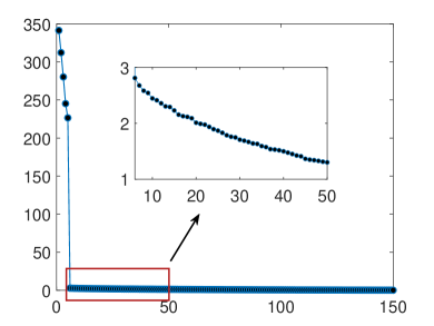
(a)

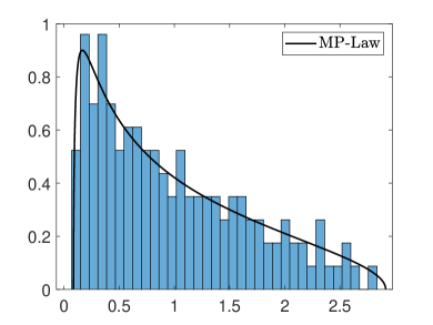
(b)

Figure 7: (a): Scree plot of the eigenvalues of the matrix $\mathbf{H}$. (b): Comparison between the empirical distribution of the non-spiked eigenvalues of $\mathbf{H}$ and the MP-Law distribution.

Supplementary materials contain the additional simulation results for Section 2.4 and some simulations for the issues raised in the section of conclusion.

References

• [1] {bbook}[author] \bauthor\bsnmAnderson, \bfnmT. W.\binitsT. W. (\byear2003). \btitleAn Introduction to Multivariate Statistical Analysis. \bpublisherJohn Wiley & Sons. \endbibitem
• [2] {barticle}[author] \bauthor\bsnmBai, \bfnmZhidong\binitsZ., \bauthor\bsnmChen, \bfnmJiaqi\binitsJ. and \bauthor\bsnmYao, \bfnmJianfeng\binitsJ. (\byear2010). \btitleOn estimation of the population spectral distribution from a high-dimensional sample covariance matrix. \bjournalAustralian & New Zealand Journal of Statistics \bvolume52 \bpages423-437. \endbibitem
• [3] {barticle}[author] \bauthor\bsnmBai, \bfnmZhidong\binitsZ., \bauthor\bsnmJiang, \bfnmDandan\binitsD., \bauthor\bsnmYao, \bfnmJianFeng\binitsJ. and \bauthor\bparticlerong \bsnmZheng, \bfnmShu\binitsS. (\byear2013). \btitleTesting linear hypotheses in high-dimensional regressions. \bjournalStatistics \bvolume47 \bpages1207 - 1223. \endbibitem
• [4] {bbook}[author] \bauthor\bsnmBai, \bfnmZhidong\binitsZ. and \bauthor\bsnmSilverstein, \bfnmJack W.\binitsJ. W. (\byear2010). \btitleSpectral Analysis of Large Dimensional Random Matrices. \bpublisherSpringer. \endbibitem
• [5] {barticle}[author] \bauthor\bsnmBai, \bfnmZhidong\binitsZ. and \bauthor\bsnmYao, \bfnmJianfeng\binitsJ. (\byear2008). \btitleCentral limit theorems for eigenvalues in a spiked population model. \bjournalAnnales de l’Institut Henri Poincaré, Probabilités et Statistiques \bvolume44 \bpages447 – 474. \bdoi10.1214/07-AIHP118 \endbibitem
• [6] {barticle}[author] \bauthor\bsnmBai, \bfnmZhidong\binitsZ. and \bauthor\bsnmYao, \bfnmJianfeng\binitsJ. (\byear2012). \btitleOn sample eigenvalues in a generalized spiked population model. \bjournalJournal of Multivariate Analysis \bvolume106 \bpages167-177. \endbibitem
• [7] {barticle}[author] \bauthor\bsnmBaik, \bfnmJinho\binitsJ., \bauthor\bsnmArous, \bfnmGérard Ben\binitsG. B. and \bauthor\bsnmPéché, \bfnmSandrine\binitsS. (\byear2005). \btitlePhase transition of the largest eigenvalue for nonnull complex sample covariance matrices. \bjournalThe Annals of Probability \bvolume33 \bpages1643 – 1697. \bdoi10.1214/009117905000000233 \endbibitem
• [8] {barticle}[author] \bauthor\bsnmBaik, \bfnmJinho\binitsJ. and \bauthor\bsnmSilverstein, \bfnmJack W.\binitsJ. W. (\byear2006). \btitleEigenvalues of large sample covariance matrices of spiked population models. \bjournalJournal of Multivariate Analysis \bvolume97 \bpages1382-1408. \endbibitem
• [9] {barticle}[author] \bauthor\bsnmBartlett, \bfnmMaurice Stevenson\binitsM. S. and \bauthor\bsnmWhite, \bfnmF. Puryer\binitsF. P. (\byear1934). \btitleThe vector representation of a sample. \bjournalMathematical Proceedings of the Cambridge Philosophical Society \bvolume30 \bpages327 - 340. \endbibitem
• [10] {bbook}[author] \bauthor\bsnmBonferroni, \bfnmC. E.\binitsC. E. (\byear1936). \btitleTeoria statistica delle classi e calcolo delle probabilità. \bseriesPubblicazioni del R. Istituto superiore di scienze economiche e commerciali di Firenze. \bpublisherSeeber. \endbibitem
• [11] {barticle}[author] \bauthor\bsnmCai, \bfnmT. Tony\binitsT. T., \bauthor\bsnmHan, \bfnmXiao\binitsX. and \bauthor\bsnmPan, \bfnmGuangming\binitsG. (\byear2020). \btitleLimiting laws for divergent spiked eigenvalues and largest nonspiked eigenvalue of sample covariance matrices. \bjournalThe Annals of Statistics \bvolume48 \bpages1255 – 1280. \bdoi10.1214/18-AOS1798 \endbibitem
• [12] {barticle}[author] \bauthor\bsnmHastie, \bfnmTrevor J.\binitsT. J., \bauthor\bsnmBuja, \bfnmAndreas\binitsA. and \bauthor\bsnmTibshirani, \bfnmRobert\binitsR. (\byear1995). \btitlePenalized Discriminant Analysis. \bjournalAnnals of Statistics \bvolume23 \bpages73-102. \endbibitem
• [13] {barticle}[author] \bauthor\bsnmJiang, \bfnmDandan\binitsD. (\byear2017). \btitleLikelihood-based tests on moderate-high-dimensional mean vectors with unequal covariance matrices. \bjournalJournal of The Korean Statistical Society \bvolume46 \bpages451-461. \endbibitem
• [14] {barticle}[author] \bauthor\bsnmJiang, \bfnmDandan\binitsD. (\byear2023). \btitleA universal test on spikes in a high-dimensional generalized spiked model and its applications. \bjournalStatistica Sinica. \bnotePreprint. \endbibitem
• [15] {barticle}[author] \bauthor\bsnmJiang, \bfnmDandan\binitsD. and \bauthor\bsnmBai, \bfnmZhidong\binitsZ. (\byear2021). \btitleGeneralized four moment theorem and an application to CLT for spiked eigenvalues of high-dimensional covariance matrices. \bjournalBernoulli \bvolume27 \bpages274 – 294. \bdoi10.3150/20-BEJ1237 \endbibitem
• [16] {barticle}[author] \bauthor\bsnmJiang, \bfnmDandan\binitsD. and \bauthor\bsnmBai, \bfnmZhidong\binitsZ. (\byear2021). \btitlePartial generalized four moment theorem revisited. \bjournalBernoulli \bvolume27 \bpages2337 – 2352. \bdoi10.3150/20-BEJ1310 \endbibitem
• [17] {barticle}[author] \bauthor\bsnmJiang, \bfnmDandan\binitsD., \bauthor\bsnmHao, \bfnmHan\binitsH., \bauthor\bsnmYang, \bfnmLu\binitsL. and \bauthor\bsnmWang, \bfnmRui\binitsR. (\byear2022). \btitleTOSE: A Fast Capacity Estimation Algorithm Based on Spike Approximations. \bjournal2022 IEEE 96th Vehicular Technology Conference (VTC2022-Fall). \endbibitem
• [18] {barticle}[author] \bauthor\bsnmJiang, \bfnmDandan\binitsD., \bauthor\bsnmHou, \bfnmZhiqiang\binitsZ. and \bauthor\bsnmHu, \bfnmJiang\binitsJ. (\byear2021). \btitleThe limits of the sample spiked eigenvalues for a high-dimensional generalized Fisher matrix and its applications. \bjournalJournal of Statistical Planning and Inference \bvolume215 \bpages208-217. \bdoihttps://doi.org/10.1016/j.jspi.2021.03.004 \endbibitem
• [19] {binproceedings}[author] \bauthor\bsnmJixiu, \bauthor\bsnmHongyan, \bfnmZhang\binitsZ., \bauthor\bsnmYue, \bfnmJin\binitsJ., \bauthor\bsnmXuting, \bfnmYan\binitsY. and \bauthor\bsnmHui, \bfnmWang\binitsW. (\byear2015). \btitleBased on SVM power quality disturbance classification algorithm. In \bbooktitleThe 27th Chinese Control and Decision Conference (2015 CCDC) \bpages3618-3621. \bdoi10.1109/CCDC.2015.7162551 \endbibitem
• [20] {barticle}[author] \bauthor\bsnmJohnstone, \bfnmIain M.\binitsI. M. (\byear2001). \btitleOn the distribution of the largest eigenvalue in principal components analysis. \bjournalThe Annals of Statistics \bvolume29 \bpages295 – 327. \bdoi10.1214/aos/1009210544 \endbibitem
• [21] {barticle}[author] \bauthor\bsnmJohnstone, \bfnmIain M.\binitsI. M. and \bauthor\bsnmOnatski, \bfnmAlexei\binitsA. (\byear2020). \btitleTesting in high-dimensional spiked models. \bjournalThe Annals of Statistics \bvolume48 \bpages1231 – 1254. \bdoi10.1214/18-AOS1697 \endbibitem
• [22] {bmisc}[author] \bauthor\bsnmKe Chen, \bfnmBo Wang\binitsB. W. \bsuffixDandan Jiang and \bauthor\bsnmWang, \bfnmHongxia\binitsH. (\byear2022). \btitleFisher Matrix Based Fault Detection for PMUs Data in Power Grids. \bnotearXiv:2208.04637. \endbibitem
• [23] {barticle}[author] \bauthor\bsnmKritchman, \bfnmShira\binitsS. and \bauthor\bsnmNadler, \bfnmBoaz\binitsB. (\byear2008). \btitleDetermining the number of components in a factor model from limited noisy data. \bjournalChemometrics and Intelligent Laboratory Systems \bvolume94 \bpages19-32. \bdoihttps://doi.org/10.1016/j.chemolab.2008.06.002 \endbibitem
• [24] {barticle}[author] \bauthor\bsnmLi, \bfnmWeiming\binitsW., \bauthor\bsnmChen, \bfnmJiaqi\binitsJ., \bauthor\bsnmQin, \bfnmYingli\binitsY., \bauthor\bsnmBai, \bfnmZhidong\binitsZ. and \bauthor\bsnmYao, \bfnmJianfeng\binitsJ. (\byear2013). \btitleEstimation of the population spectral distribution from a large dimensional sample covariance matrix. \bjournalJournal of Statistical Planning and Inference \bvolume143 \bpages1887-1897. \bdoihttps://doi.org/10.1016/j.jspi.2013.06.017 \endbibitem
• [25] {barticle}[author] \bauthor\bsnmLi, \bfnmWeiming\binitsW. and \bauthor\bsnmYao, \bfnmJianfeng\binitsJ. (\byear2015). \btitleOn generalized expectation-based estimation of a population spectral distribution from high-dimensional data. \bjournalAnnals of the Institute of Statistical Mathematics \bvolume67 \bpages359-373. \bdoi10.1007/s10463-014-0452-2 \endbibitem
• [26] {barticle}[author] \bauthor\bsnmPassemier, \bfnmDamien\binitsD., \bauthor\bsnmLi, \bfnmZhaoyuan\binitsZ. and \bauthor\bsnmYao, \bfnmJianfeng\binitsJ. (\byear2017). \btitleOn estimation of the noise variance in high dimensional probabilistic principal component analysis. \bjournalJournal of the Royal Statistical Society Series B \bvolume79 \bpages51-67. \endbibitem
• [27] {barticle}[author] \bauthor\bsnmPassemier, \bfnmDamien\binitsD. and \bauthor\bsnmYao, \bfnmJianfeng\binitsJ. (\byear2012). \btitleOn determining the number of spikes in a high-dimensional spiked population model. \bjournalRand. Matr. Theor. Appl. \bvolume1 \bpagesarticle 1150002. \endbibitem
• [28] {barticle}[author] \bauthor\bsnmPaul, \bfnmDebashis\binitsD. (\byear2007). \btitleAsymptotics of sample eigenstructure for a large dimensional spiked covariance model. \bjournalStatistica Sinica \bvolume17 \bpages1617-1642. \endbibitem
• [29] {barticle}[author] \bauthor\bsnmRao, \bfnmN. Raj\binitsN. R., \bauthor\bsnmMingo, \bfnmJames A.\binitsJ. A., \bauthor\bsnmSpeicher, \bfnmRoland\binitsR. and \bauthor\bsnmEdelman, \bfnmAlan\binitsA. (\byear2008). \btitleStatistical eigen-inference from large Wishart matrices. \bjournalThe Annals of Statistics \bvolume36 \bpages2850 – 2885. \bdoi10.1214/07-AOS583 \endbibitem
• [30] {barticle}[author] \bauthor\bsnmTelatar, \bfnmEmre\binitsE. (\byear1999). \btitleCapacity of Multi‐antenna Gaussian Channels. \bjournalEuropean Transactions on Telecommunications \bvolume10 \bpages585-595. \endbibitem
• [31] {barticle}[author] \bauthor\bsnmUlfarsson, \bfnmM. O.\binitsM. O. and \bauthor\bsnmSolo, \bfnmV.\binitsV. (\byear2008). \btitleDimension Estimation in Noisy PCA With SURE and Random Matrix Theory. \bjournalTrans. Sig. Proc. \bvolume56 \bpages5804–5816. \bdoi10.1109/TSP.2008.2005865 \endbibitem
• [32] {barticle}[author] \bauthor\bsnmWang, \bfnmBo\binitsB., \bauthor\bsnmWang, \bfnmHongxia\binitsH., \bauthor\bsnmZhang, \bfnmLiming\binitsL., \bauthor\bsnmZhu, \bfnmDanlei\binitsD., \bauthor\bsnmLin, \bfnmDongxu\binitsD. and \bauthor\bsnmWan, \bfnmShaohua\binitsS. (\byear2019). \btitleA Data-Driven Method to Detect and Localize the Single-Phase Grounding Fault in Distribution Network Based on Synchronized Phasor Measurement. \bjournalEURASIP J. Wirel. Commun. Netw. \bvolume2019 \bpages1–13. \bdoi10.1186/s13638-019-1521-2 \endbibitem
• [33] {barticle}[author] \bauthor\bsnmWang, \bfnmQinwen\binitsQ. and \bauthor\bsnmYao, \bfnmJianfeng\binitsJ. (\byear2017). \btitleExtreme eigenvalues of large-dimensional spiked Fisher matrices with application. \bjournalThe Annals of Statistics \bvolume45 \bpages415 – 460. \bdoi10.1214/16-AOS1463 \endbibitem
• [34] {bmisc}[author] \bauthor\bsnmWang, \bfnmRui\binitsR. and \bauthor\bsnmJiang, \bfnmDandan\binitsD. (\byear2022). \btitleDetermining the number of factors in a large-dimensional generalised factor model. \bnotearXiv:2203.14236. \endbibitem
• [35] {barticle}[author] \bauthor\bsnmWang, \bfnmWeichen\binitsW. and \bauthor\bsnmFan, \bfnmJianqing\binitsJ. (\byear2017). \btitleAsymptotics of empirical eigenstructure for high dimensional spiked covariance. \bjournalThe Annals of Statistics \bvolume45 \bpages1342-1374. \endbibitem
• [36] {barticle}[author] \bauthor\bsnmWilks, \bfnmS. S.\binitsS. S. (\byear1932). \btitleCertain generalizations in the analysis of variance. \bjournalBiometrika \bvolume24 \bpages471-494. \bdoi10.1093/biomet/24.3-4.471 \endbibitem
• [37] {barticle}[author] \bauthor\bsnmWilks, \bfnmS. S.\binitsS. S. (\byear1934). \btitleMoment-Generating Operators for Determinants of Product Moments in Samples from a Normal System. \bjournalAnnals of Mathematics \bvolume35 \bpages312–340. \endbibitem
• [38] {barticle}[author] \bauthor\bsnmXie, \bfnmJunshan\binitsJ., \bauthor\bsnmZeng, \bfnmYicheng\binitsY. and \bauthor\bsnmZhu, \bfnmLixing\binitsL. (\byear2021). \btitleLimiting laws for extreme eigenvalues of large-dimensional spiked Fisher matrices with a divergent number of spikes. \bjournalJournal of Multivariate Analysis \bvolume184 \bpages104742. \bdoihttps://doi.org/10.1016/j.jmva.2021.104742 \endbibitem
• [39] {barticle}[author] \bauthor\bsnmZeng, \bfnmYicheng\binitsY. and \bauthor\bsnmZhu, \bfnmLixing\binitsL. (\byear2022). \btitleOrder Determination for Spiked Type Models. \bjournalStatistica Sinica \bpages1633-1659. \endbibitem
• [40] {barticle}[author] \bauthor\bsnmZeng, \bfnmYicheng\binitsY. and \bauthor\bsnmZhu, \bfnmLixing\binitsL. (\byear2023). \btitleOrder determination for spiked-type models with a divergent number of spikes. \bjournalComputational Statistics & Data Analysis \bpages107704. \bdoihttps://doi.org/10.1016/j.csda.2023.107704 \endbibitem
• [41] {barticle}[author] \bauthor\bsnmZheng, \bfnmKanglin\binitsK., \bauthor\bsnmGeng, \bfnmZengwei\binitsZ., \bauthor\bsnmWang, \bfnmHongxia\binitsH., \bauthor\bsnmMa, \bfnmFuqi\binitsF. and \bauthor\bsnmZhang, \bfnmGege\binitsG. (\byear2019). \btitleSingle-phase Grounding Fault Detection and Localization based on Big Data From Synchronized Phasor Measurement. \bjournalPower System and Clean Energy \bvolume36 \bpages50–56. \endbibitem
• [42] {barticle}[author] \bauthor\bsnmZheng, \bfnmShurong\binitsS. (\byear2012). \btitleCentral limit theorems for linear spectral statistics of large dimensional F-matrices. \bjournalAnnales de l’Institut Henri Poincaré, Probabilités et Statistiques \bvolume48 \bpages444 -476. \bdoi10.1214/11-AIHP414 \endbibitem
• [43] {barticle}[author] \bauthor\bsnmZheng, \bfnmShurong\binitsS., \bauthor\bsnmBai, \bfnmZhidong\binitsZ. and \bauthor\bsnmYao, \bfnmJianfeng\binitsJ. (\byear2015). \btitleSubstitution principle for CLT of linear spectral statistics of high-dimensional sample covariance matrices with applications to hypothesis testing. \bjournalThe Annals of Statistics \bvolume43 \bpages546 – 591. \bdoi10.1214/14-AOS1292 \endbibitem
• [44] {barticle}[author] \bauthor\bsnmZheng, \bfnmShurong\binitsS., \bauthor\bsnmBai, \bfnmZhidong\binitsZ. and \bauthor\bsnmYao, \bfnmJianfeng\binitsJ. (\byear2017). \btitleCLT for eigenvalue statistics of large-dimensional general Fisher matrices with applications. \bjournalBernoulli \bvolume23 \bpages1130-1178. \endbibitem