Navier-Stokes bounds and scaling for compact trefoils in $(2\ell\pi)^{3}$ domains.

Abstract

Over a wide range of viscosities, a perturbed trefoil vortex knot generates Reynolds number independent finite-time energy dissipation $\Delta E_{\epsilon}$ (1) with evidence for a transient Kolmogorov spectra at the highest Reynolds number. Satisfying one definition for a dissipation anomaly. To cover the required range of Reynolds numbers, factors of $\nu^{1/4}$ must be considered for both the largest scale $L$, the size of the periodic domain, which increases as $L\sim\nu^{-1/4}$, and vorticity moments at the the earliest times, which converge when scaled as $\nu^{1/4}\Omega_{m}$, including $m=9,\infty$ at times $t_{\infty}<\dots<t_{m}\dots t_{1}=t_{x}$. The $\nu^{1/4}$ scaling ends at $t=t_{x}$ with convergence of $\sqrt{\nu}Z(t)$, $Z=L^{3}\Omega_{1}^{2}$ being the volume-integrated enstrophy, after which the growth of $Z(t)$ accelerates until there is approximate convergence of the dissipation rates $\epsilon=\nu Z$ at $t\sim t_{\epsilon}\sim 2t_{x}$. This continues long enough to generate a dissipation anomaly with finite $\Delta E_{\epsilon}$ (1). To achieve the convergence of $\sqrt{\nu}Z(t)$ at $t_{x}$, $L$ is increased from $4\pi$ to $12\pi$, meaning that the following restriction must be addressed: That $\nu\neq 0$ Navier-Stokes solutions in $(2\pi)^{3}$ periodic domains are bounded by their $\nu\equiv 0$ Euler solutions as $\nu\to 0$ for $\nu<\nu_{s}$, with the bounding critical viscosities $\nu_{s}$ determined using Sobolev space analysis. By rescaling the original Sobolev space result in $(2\pi)^{3}$ into larger $(2\ell\pi)^{3}$ domains, a reduction in the bounding critical viscosities $\nu_{s}$ can be shown which allows growth of $Z(t)$ in those domains.

1 Background

Finite-energy dissipation in large Reynolds number geophysical and engineering applications is ubiquitous. That is, for systems that can be modeled by the incompressible Navier-Stokes equations, a dissipation anomaly with finite $\Delta E_{\epsilon}$ always forms, defined as

$$\Delta E_{\epsilon}=\int_{0}^{T_{\epsilon}}\epsilon\,dt>0\quad\mbox{in a finite time }t_{\epsilon}$$ (1)

where the energy dissipation rate is $\epsilon=\nu Z$, $Z=V_{\ell}\Omega_{1}^{2}$ is the volume-integrated enstrophy, that is the integral of its density $\zeta=\omega^{2}$ over the domain $V_{\ell}=(2\ell\pi)^{3}$. With $\Omega_{1}$ being the first of a hierarchy of $\Omega_{m}$ scaled vorticity moments (6).

However, generating unforced, finite $\Delta E_{\epsilon}$ from high Reynolds number numerical simulations has proven daunting. Daunting because for the usual smooth initial states, as the viscosity is decreased, and Reynolds number increases, the convergence and then persistence of a high energy dissipation rates has never been achieved.

It is on that basis that it has been argued that there might be some small scale physics missing from the Navier-Stokes equations (Eyink & Jafari, 2022). One argument comes from applied analysis of the Navier-Stokes equations, but is largely unknown to the general fluid dynamics community This is that with identical Euler $u(0)$ and Navier-Stokes $v(0)$ initial states in $V_{1}=(2\pi)^{3}$ domains, as the viscosity $\nu\to 0$, the $\nu\equiv 0$ solutions $u(t)$ always bound $\nu\neq 0$ Navier-Stokes solutions $v(t)$ (Constantin, 1986). This applies only when the viscosity is below critical values, $\nu<\nu_{s}$, with the $\nu_{s}$ dependent upon higher-order Euler $H^{s}$ Sobolev norms (23). Specifically, in the original proof, time-integrals of the higher-order, $s\geq 3$, Sobolev norms $H^{s}(u)$ are used. With additional embedding theorems (Robinson et al., 2016) this leads to the conclusion that the dissipation rate $\epsilon=\nu Z\to 0$ as $\nu\to 0$, unless there are singularities of either the Navier-Stokes or Euler equations.

This $(2\pi)^{3}$ Sobolev space result might explain why initial value (Cauchy) calculations done in $(2\pi)^{3}$ domain consistently fail to generate evidence for a dissipation anomaly with finite $\Delta E_{\epsilon}$ (1) (Yao & Hussain, 2022). And perhaps why it is so difficult for forced calculations to increase $\Delta E_{\epsilon}$ (1) when the Reynolds numbers are increased as in Iyer et al. (2022).

An exception to this trend is a set of perturbed trefoil vortex knot simulations of Kerr (2018b) that find evidence for finite $\Delta E_{\epsilon}$ at $t_{\epsilon}\sim 96$ as $\nu$ decreases. But a pre-cursor, with temporal convergence of $\sqrt{\nu}Z(t)$ at an earlier fixed time of $t_{x}\approx 40$ can be maintained only if the size of the computational domain $V_{\ell}$ increases as the viscosity decreases (Kerr, 2018a). This is shown in Fig. 1, with two $\nu=3.125\times 10^{-5}$ curves included, $V_{\ell}=(4\pi)^{3}$ to show the effect if $V_{\ell}$ is not increased and $V_{\ell}=(6\pi)^{3}$ for when it is. To compare calculations in different domains requires a compact initial state. Meaning that both the velocity $u$ and vorticity $\omega$ fields go to zero at large $\rho$ (13) sufficiently rapidly. A trefoil vortex knot is ideal because it is compact, can be isolated from the boundaries and interesting because it has finite, non-trivial helicity.

Figure 3b shows that when the Reynolds numbers in larger domains is higher and extended in time, the dissipation rates $\epsilon=\nu Z$ also converge over a finite period, providing evidence for finite-time $\Delta E_{\epsilon}$. Most recently, three-fold symmetric trefoils with different initial core profiles have been simulated in strictly $V_{1}=(2\pi)^{3}$ domains. For the better, algebraic profiles, vortex sheets grow out of the original vortices and generate enstrophy growth that is consistent with finite-time $\Delta E_{\epsilon}$, despite the restrictions due to the domain size and symmetry. Figure 5 shows the growth of vortex sheets for one of the present calculations and figures 7 and 7 show how those sheets then start to roll-up.

Is the domain size dependence of $\sqrt{\nu}Z(t)$ convergence in figure 1 consistent with restrictions of the original $(2\pi)^{3}$ mathematics (Constantin, 1986)? In Appendix A, those restrictions are relaxed by extending the mathematics for the Sobolev space critical viscosities $\nu_{s}$ to larger domains with $V_{\ell}=(2\ell\pi)^{3}$, $\ell>1$. To determine the $\nu_{s}$ in the larger domain, the velocities in the $V_{\ell}$ domain are rescaled into the smaller $(2\pi)^{3}$ domain, such that the original timescales and Reynolds numbers are retained. Then the known $\nu_{s}$ bounds in a $(2\pi)^{3}$ domain (Constantin, 1986) are used to find the critical viscosities $\nu_{s_{2\pi}}$ using the $H^{s_{2\pi}}$ norms in the $(2\pi)^{3}$ domain. Finally, those $\nu_{s_{2\pi}}$ are rescaled back to the $V_{\ell}$ domain, with the resulting $\nu_{s}$ decreasing as $\ell$ increases. This result can explain how the trefoil results with convergent $\sqrt{\nu}Z(t)$, and then convergent $\epsilon=\nu Z(t)$, can be allowed by the mathematics. And if extended further by taking $\ell\to\infty$, one might be able identify limiting behaviour in $\mathbb{R}^{3}$, known as whole space.

The mathematics in a $V_{1}=(2\pi)^{3}$ domain comes from subtracting the Euler equations for $u$ from the Navier-Stokes equations for $v$, followed by detailed Sobolev space analysis of the resulting $w=v-u$ equations. That analysis begins by taking the inner product (21) between $w$ and its equation then reconfiguring this into a set of nonlinear time inequalities (42) whose right-hand-sides consist of a viscous Euler forcing , a cubic nonlinearity and a linear term, which is removed by using integrating factors (43). Because the result (44) uses rescaled Euler norms (28) in its coefficients and integrating factors, some discussion of a recent version of the original $(2\pi)^{3}$ method (Constantin, 1986) is required.

Kerr (2018b) previously determined that domains needed to be increased as $\ell\sim\nu^{-1/4}$. By recognizing that $\sqrt{\nu}Z=(\nu^{1/4}V_{\ell}^{1/2}\Omega_{1})^{2}$, it has now been found that for two additional $m>1$, $m\!=\!9$ and $\infty$, that the $\nu^{1/4}\Omega_{m}(t)$ of each temporally converges to its own $t_{m}\lesssim t_{x}$. This is discussed in section 2.1

The paper is organized as follows. After the equations are introduced, what has inspired this paper, the empirical $\sqrt{\nu}Z(t)$ convergence at the first reconnection $t=t_{x}$, is mentioned, noting that $Z=V\Omega_{1}^{2}$. Then the extended numerical results for both $1/(\sqrt{\nu}Z(t))^{1/2}$ and $\epsilon(t)={\nu}Z$ scaling are given, including evidence for a dissipation anomaly and turbulent-like spectra. This is followed by two more examples of $t\lesssim t_{x}$, $\nu^{1/4}\Omega_{m}(t)$ convergence. Finally, the dissipation range vortical structures that characterize the $t\lesssim t_{x}$ phase are given in section 3. The appendix begins by stating the necessary fundamental of Sobolev $H^{s}$, analysis required for extending the $(2\pi)^{3}$ analysis for bounds upon growth. Then presents the extension to larger domains that allows relaxation of the critical viscosity $\nu_{s}$ bounds upon small viscosities, which in turn allows convergence of the dissipation rate $\epsilon\nu Z$ as $\nu$ decreases.

1.1 Governing equations

This paper uses the incompressible viscous $\nu\sim Re^{-1}\neq 0$ Navier-Stokes velocity equations

$$\frac{\partial\mbox{\boldmath$v$}}{\partial t}+({\mbox{\boldmath$v$}}\cdot\nabla){\mbox{\boldmath$v$}}=-\nabla p+\underbrace{\nu\triangle{\mbox{\boldmath$v$}}}_{\rm viscous~{}drag},\quad\nabla\cdot{\mbox{\boldmath$v$}}=0\,,$$ (2)

the inviscid $\nu\equiv 0$ Euler equations

$$\frac{\partial\mbox{\boldmath$u$}}{\partial t}+({\mbox{\boldmath$u$}}\cdot\nabla){\mbox{\boldmath$u$}}=-\nabla p\,,$$ (3)

and the equation for their difference $\mbox{\boldmath$w$}=\mbox{\boldmath$v$}-\mbox{\boldmath$u$}$, which by replacing $v$ by $\mbox{\boldmath$w$}+\mbox{\boldmath$u$}$ throughout becomes

$$\mbox{\boldmath$w$}_{t}+\nu\Delta\mbox{\boldmath$w$}=-\nu\Delta\mbox{\boldmath$u$}-\underbrace{(\mbox{\boldmath$w$}\cdot\nabla)\mbox{\boldmath$w$}}_{B_{NL}(w,w)}-\underbrace{(\mbox{\boldmath$u$}\cdot\nabla)\mbox{\boldmath$w$}}_{B_{NL}(u,w)}-\underbrace{(\mbox{\boldmath$w$}\cdot\nabla)\mbox{\boldmath$u$}}_{B_{NL}(w,u)}-\nabla p_{w}-\nabla p_{u}\,.$$ (4)

The Constantin & Foias (1988) notation $B_{NL}(u,v)=(\mbox{\boldmath$u$}\cdot\nabla)\mbox{\boldmath$v$}$ has been added to emphasize the similarities between how the three nonlinear terms are treated in section A.5.

The equation for the vorticity $\mbox{\boldmath$\omega$}=\nabla\times\mbox{\boldmath$v$}$ is

$$\frac{\partial\mbox{\boldmath$\omega$}}{\partial t}+({\mbox{\boldmath$v$}}\cdot\nabla){\mbox{\boldmath$\omega$}}=({\mbox{\boldmath$\omega$}}\cdot\nabla){\mbox{\boldmath$v$}}+\nu\triangle{\mbox{\boldmath$\omega$}},\qquad\nabla\cdot{\mbox{\boldmath$\omega$}}=0\,.$$ (5)

and in fixed domains $V$ the vorticity moments obey this hierarchy

$$\Omega_{m}(t)=\left(V^{-1}\int_{\cal V}|\omega|^{2m}dV\right)^{1/2m}\quad\text{with}\quad\Omega_{1}(t)\leq\Omega_{2}(t)\leq\dots\Omega_{m}(t)\leq\dots\leq\Omega_{\infty}(t)$$ (6)

This ordering represents a type of Hölder inequality and neglects the $V$-dependent constants. Note that $\Omega_{\infty}=\|\omega\|_{\infty}$ is at the high end, and at the other end, the volume-integrated enstrophy can be written as $Z(t)=V\Omega_{1}^{2}(t)$. These moments, scaled by characteristic frequencies, have been used in several recent papers (Kerr, 2013a, b; Donzis et al., 2013).

For a compact vortex knot, the circulations $\Gamma_{i}$ about its vortex structures are:

$$\Gamma_{i}=\oint_{{\cal C}_{i}}\mbox{\boldmath$v$}_{i}\cdot\mbox{\boldmath$r$}_{i}\quad{\rm where}\quad\mbox{\boldmath$r$}_{i}~{}~{}\mbox{is a closed loop about}~{}~{}{\cal C}_{i}\,.$$ (7)

Dimensionally, for a vortex knot of size $r_{f}$ with velocity scale of $U$, the circulation goes as $\Gamma\sim Ur_{f}$. In vortex dynamics the circulation Reynolds number $R_{\Gamma}=\Gamma/\nu$ is widely used and for a vortex knot of size $r_{f}$, the nonlinear and viscous timescales are respectively:

$$t_{NL}=r_{f}^{2}/\Gamma\quad\text{and}\quad t_{\nu}=r_{f}^{2}/\nu\,.$$ (8)

The rescaling that will be applied to $V_{\ell}=(2\ell\pi)^{3}$ domains shrinks $\ell$ to 1, with $U$ and $\nu$ rescaled such that: The Reynolds number is invariant; all ratios of length scales are invariant; the time-scales are invariant; and the original physics is preserved.

Three local densities are used. The energy density $e=\mbox{$\frac{1}{2}$}u^{2}$, the enstrophy density $\zeta=\omega^{2}$ and the helicity density $h=\mbox{\boldmath$u$}\cdot\mbox{\boldmath$\omega$}$. Their budget equations, with their global integrals, are:

$$\frac{\partial e}{\partial t}+({\mbox{\boldmath$u$}}\cdot\nabla)e=-\nabla\cdot(\mbox{\boldmath$u$}p)+\nu\triangle e-\underbrace{\nu(\nabla\mbox{\boldmath$u$})^{2}}_{\epsilon={\rm dissipation}=\nu Z},~{}E_{e}=\mbox{$\frac{1}{2}$}\int_{{\cal V}_{\ell}}\mbox{\boldmath$u$}^{2}dV\,;$$ (9)

$$\frac{\partial\zeta}{\partial t}+({\mbox{\boldmath$u$}}\cdot\nabla)|\mbox{\boldmath$\omega$}|^{2}=\underbrace{2\mbox{\boldmath$\omega$}\mbox{\boldmath$S$}\mbox{\boldmath$\omega$}}_{\zeta_{p}={\rm production}}+\nu\triangle|\mbox{\boldmath$\omega$}|^{2}-\underbrace{2\nu(\nabla\mbox{\boldmath$\omega$})^{2}}_{\epsilon_{\omega}=Z-{\rm dissipation}},~{}Z=\int_{{\cal V}_{\ell}}\mbox{\boldmath$\omega$}^{2}dV\,;$$ (10)

$$\frac{\partial h}{\partial t}+({\mbox{\boldmath$u$}}\cdot\nabla)h=\underbrace{-\mbox{\boldmath$\omega$}\cdot\nabla\Pi}_{h_{f}=\omega-{\rm transport}}+\underbrace{\nu\mbox{\boldmath$\triangle$}h}_{\nu-{\rm transport}}-\underbrace{2\nu{\rm tr}(\nabla\mbox{\boldmath$\omega$}\cdot\nabla\mbox{\boldmath$u$}^{T})}_{\epsilon_{h}={\cal H}-{\rm dissipation}}\,,\,{\cal H}=\int\mbox{\boldmath$u$}\cdot\mbox{\boldmath$\omega$}dV\,.$$ (11)

Note that $\Pi=p-\mbox{$\frac{1}{2}$}\mbox{\boldmath$u$}^{2}\neq p_{h}$ and is not the pressure head $p_{h}=p+\mbox{$\frac{1}{2}$}\mbox{\boldmath$u$}^{2}$.

In this paper the primary norms are related to the energy and enstrophy equations. The helicity budget is included because the helicity density $h$ is mapped onto the vorticity isosurfaces for potential comparisons with the isosurfaces of the three-fold symmetric trefoils (Kerr, 2023), where its budget equation is discussed in detail.

Under $\nu\equiv 0$ Euler, both $E_{e}$ and ${\cal H}$, the global helicity, are conserved. With the pressure gradients affecting only their local Lagrangian densities $e$ and $h$. In contrast, the global enstrophy $Z$ is not an invariant, but grows in figure 1 due to vortex stretching, as discussed in section 2. $E_{e}$ and $Z$ can be recast in terms to the first two Sobolev norms, $H^{0}$ and $H^{1}$, defined below (24). Due to vortex stretching, initially all $H^{s}$, $s>1$, tend to grow.

1.2 Trefoil initial conditon

The trefoil vortex knot in this paper at $t=0$ is defined as follows:

• $\mbox{\boldmath$\xi$}_{0}(\phi)=[x(\phi),y(\phi),z(\phi)$ defines the centerline trajectory of a closed double loop over $\phi=1:4\pi$ with $a=0.5$, $w=1.5$, a characteristic size of $r_{f}=2$ and a perturbation of $r_{1}=0.25$.

  $$\begin{array}[]{rrl}&x(\phi)=&r(\phi)\cos(\alpha)\\ &y(\phi)=&r(\phi)\sin(\alpha)\qquad z(\phi)=a\cos(\alpha)\\ {\rm where}&r(\phi)=&r_{f}+r_{1}a\cos(\phi)+a\sin(w\phi+\phi_{0})\\ &\alpha=&\phi+a\cos(w\phi+\phi_{0})/(wr_{f})\\ {\rm and}&r_{e}=&(\Gamma/(\pi\omega_{m}))^{1/2}\mbox{ the effective radius.}\end{array}$$ (12)

• The vorticity profile $|\omega(\rho)|$ uses the distance $\rho$ between a given mesh point $x$ and the nearest point on the trajectory $\mbox{\boldmath$\xi$}_{0}(\phi)$: $\rho=|\mbox{\boldmath$x$}-\mbox{\boldmath$\xi$}_{0}(\phi)|$. The profile used here is algebraic (13)

  $$\omega_{\mbox{raw}}(\rho)=\omega_{o}\frac{(r_{o}^{2})^{p_{r}}}{(\rho^{2}+r_{o}^{2})^{p_{r}}}\,.$$ (13)

  with a power-law of $p_{r}=1$, a radius of $r_{o}=0.25$ and a centerline vorticity before projection of $\omega_{o}\approx 1.26$. This profile is mapped onto the Cartesian mesh and made incompressible as described previously (Kerr, 2018a, 2023). The final $\omega_{o}$ is chosen in each case so that the circulation is always $\Gamma=0.505$ (7), $\|\omega(0)\|_{\infty}=1$ and the nonlinear timescale is $t_{NL}=r_{f}^{2}/\Gamma=8$ (12).

1.3 Reconnection scaling with $\sqrt{\nu}Z$

What has been found previously for numerical trefoils (Kerr, 2018a, b, 2023) is that $\sqrt{\nu}Z(t)$ converges at a fixed time $t_{x}$ for $\nu$ greater than an empirically determined critical value $\nu_{c}$ if the periodic domain $V_{\ell}=(2\ell\pi)^{3}$ is fixed. Moreover, if the domain size increases as $\nu$ decreases, the convergence can be maintained. Figure 1 uses extensions of those 2018 results with better resolution for all cases shown, and for the $\nu=7.8\times 10^{-6}$ case in a $(9\pi)^{3}$ domain, an extension in time.

The $t_{x}=40$ convergence of $\sqrt{\nu}Z(t)$ is found for $\nu=5\times 10^{-4}$ to $2\times 10^{-6}$, a factor of 256, with $\ell$ increasing by a factor of 4 over the original $\ell=1.5$, $\nu=5\times 10^{-4}$ calculation (Kerr, 2018a), with the domain size increasing by a factor of $4^{3}=64$.

Two simulations with $\nu=3.1\times 10^{-5}$ illustrate what happens if the domain is not increased as $\nu$ decreases. The brown-+ curve, done in a $\ell=2$, $(4\pi)^{3}$ domain passes below $\sqrt{\nu}Z=0.15$ at $t=40$. The green $\triangle$ curve was done in a $\ell=3$, $(6\pi)^{3}$ domain and passes through $\sqrt{\nu}Z=0.15$ at $t=40$. Suggesting that for this initial condition in a $(4\pi)^{3}$ domain, $\nu_{c}\sim 3.1\times 10^{-5}$. To maintain the $\sqrt{\nu}Z(t)$ convergence as the viscosity $\nu$ is decreased and the Reynolds number increased further, $\nu_{c}$ had to be decreased by increasing the domain parameter $\ell$ repeatedly (Kerr, 2018a, b). This practice was continued several times, providing empirical dependence for how a critical length scale $\ell_{c}$ depends upon $\nu$:

$$\ell_{c}\sim\nu^{-1/4},\quad\text{or}\quad\nu_{c}\sim\ell^{-4}\,.$$ (14)

Raising this question: what is origin of the dependence of the critical viscosities $\nu_{c}(\ell)$ upon $\ell$ and $\nu^{-1/4}$? Section 2.1 discusses the ubiquitous nature of the $\nu^{1/4}$ scaling and section 3 the importance of vortex sheets. However, trefoils are too complicated to be able to see the underlying dynamics, which is being done using initial orthogonal vortices.

Note that convergence of $\sqrt{\nu}Z(t)$ as $\nu$ decreases is not convergence of the energy dissipation rate $\epsilon=\nu Z$, which comes later at the time $t_{\epsilon}\approx 2t_{x}$ as shown in figure 3b.

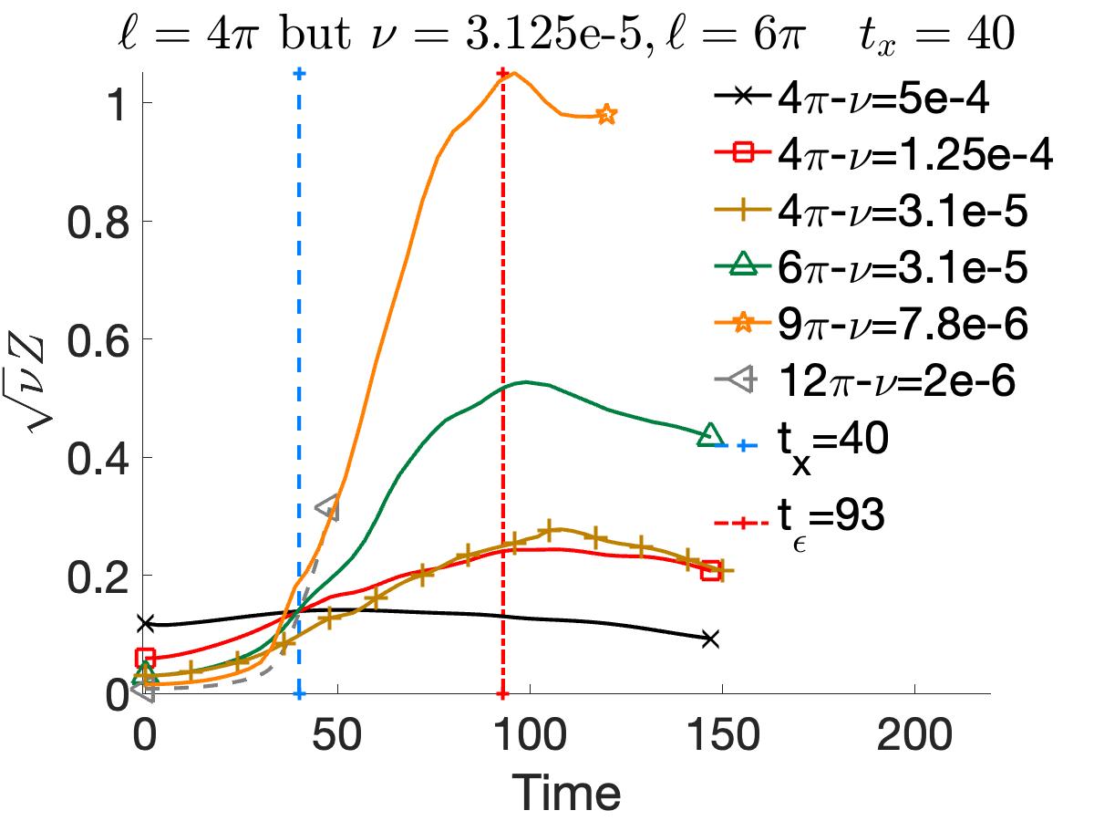
Figure 1: Time evolution of the reconnection enstrophy $\sqrt{\nu}Z$ from (Kerr, 2018b) with the $\nu=7.8\times 10^{-6}$ case (orange $\star$) extended in time. Note that all the curves, except the brown-+ curve, cross at $t_{x}=40$ with $\sqrt{\nu}Z(t_{x})=B_{x}^{-2}=0.14$ (15). $t_{x}=40$ was previously identified as the end of the first reconnection (Kerr, 2018b). The brown-+ curve is from a $\nu=3.125\times 10^{-5}$, $(4\pi)^{3}$ calculation, the same domain as the lower $\nu<3.125\times 10^{-5}$viscous cases, but $\sqrt{\nu}Z(t=40)\neq 0.14$. Unlike the $\nu=3.125\times 10^{-5}$ green curve that was run in a $(6\pi)^{3}$, with $\sqrt{\nu}Z(40)=0.14$. The line at $t_{\epsilon}=93$ is when plots of the dissipation $\epsilon=\nu Z$ approximately cross in figure 3b.

2 Reconnection phase scaling and spectra

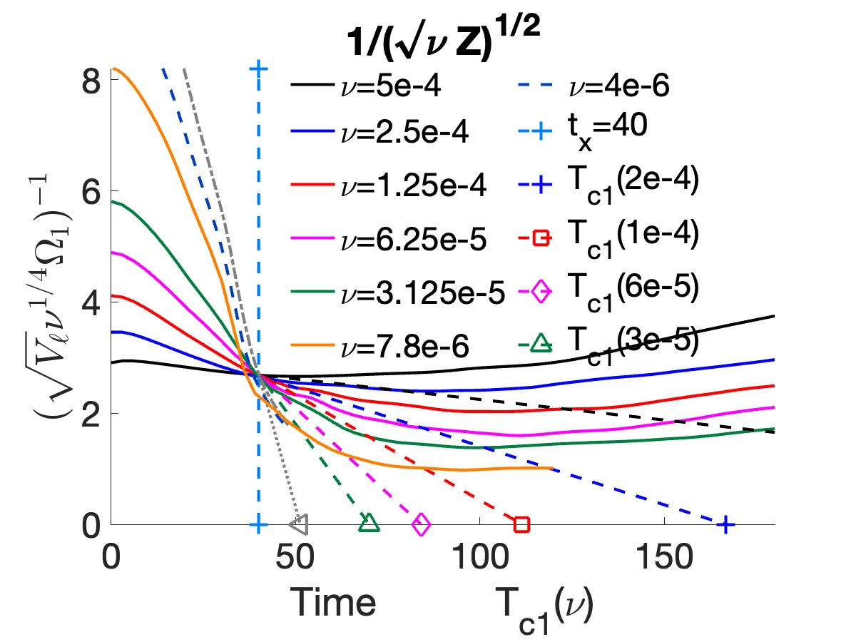
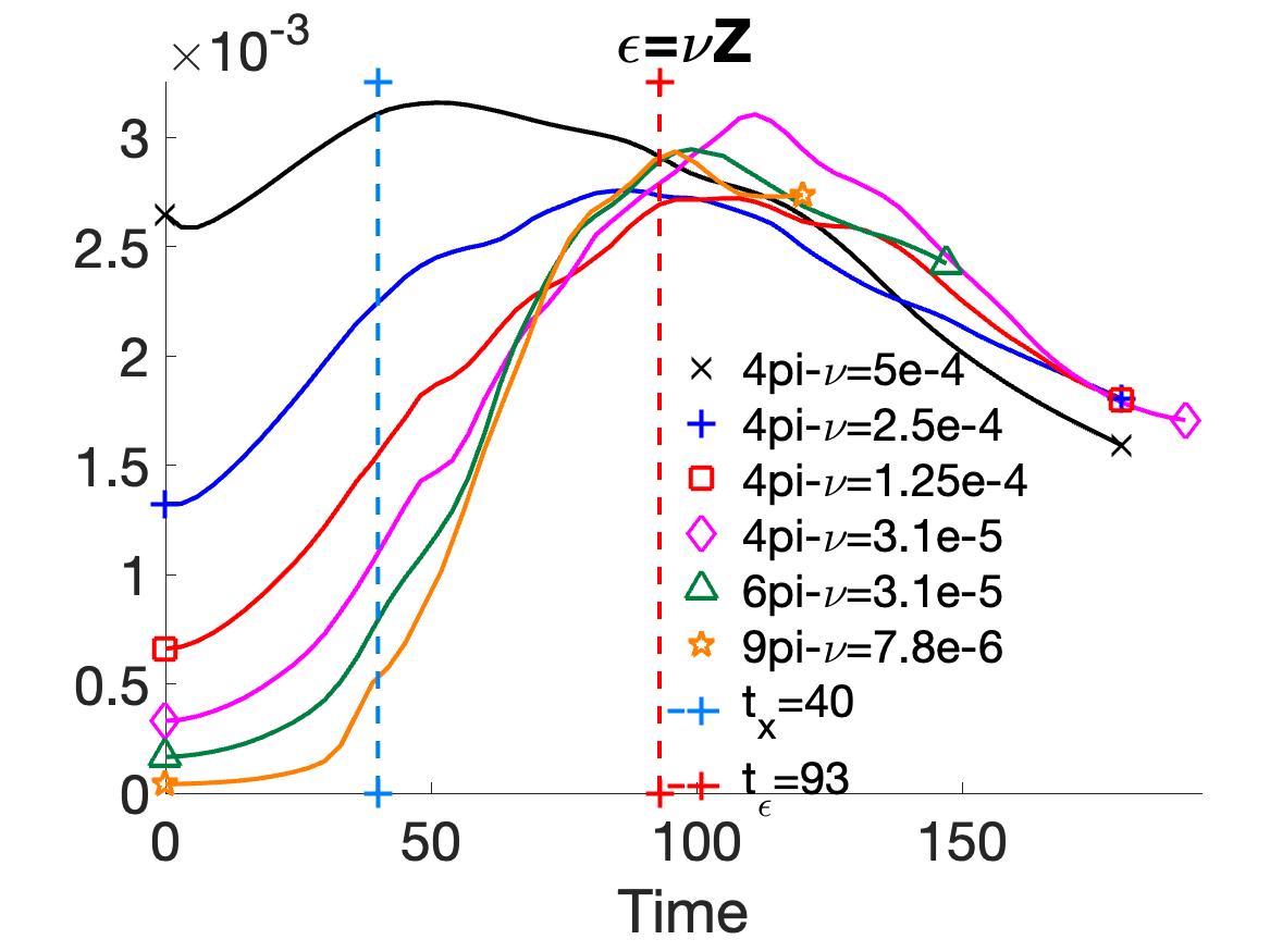
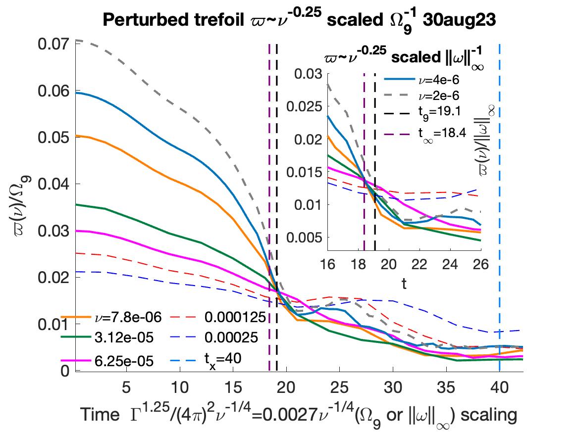
Figure 2: These figures show two alternative viscosity-based rescalings of the enstrophy $Z$. (a) By rescaling $B(\nu,t)^{-1}=1/(\sqrt{\nu}Z(t))^{1/2}$ (15) as $(\sqrt{V}\nu^{1/4}\Omega_{1})^{-1}$ (6), decreasing inversely-linear, $\sim(t_{x}-t)$ behavior, is demonstrated for $t\lesssim t_{x}$, with strong $t_{x}=40$ convergence over a wide range of viscosities. With $\nu=7.8\times 10^{-6}$ is being the slight exception because it was run in a $(9\pi)^{3}$ domain. Effective singular times $T_{c1}(\nu)$ (17) are indicated by long-dashed lines with symbols that are linear extensions of the $t\lesssim t_{x}$ $B(\nu,t)^{-1}$. Empirically, increases in the domain sizes $(2\ell\pi)^{3}$, with $\ell(\nu)\sim\nu^{-1/4}$, are required to maintain the $t\lesssim t_{x}$ linear scaling as $\nu$ decreases. (b) The dissipation rate $\epsilon=\nu Z$ for six cases, $\nu=5\times 10^{-4}$ to $7.8\times 10^{-6}$, showing approximate convergence of the dissipation rates at $t_{\epsilon}\approx 93\approx 2t_{x}$ for an extended period. These trends are consistent with the formation of a dissipation anomaly (1), that is finite energy dissipation in a finite time as $\nu$ decreases.

Figure 3: $\varpi(\nu)/\Omega_{9}(t)$ (main frame) and $\varpi(\nu)/\|\omega(t)\|_{\infty}$ (inset)
versus time for $t\!\leq\!42$, $\varpi(\nu)\!=\!\Gamma^{1.25}\nu^{-1/4}/(4\pi)^{2}$
$\!\sim\!\nu^{-1/4}$. Because
$\|\omega(t=0)\|_{\infty}\!=\!1$, the $\Omega_{9}$ are normalized such that $\Omega_{9}(t=0)=1$ irrespective of the size of the domain. Recall that the end of the first reconnection is indicated by when the $\sqrt{\nu}Z$ converge at $t_{x}=40$ in figure 3a. For $\nu\!=\!6.25\!\times\!10^{-5}$ to $\nu\!=\!4\!\times\!10^{-6}$, the $\varpi(\nu)/\Omega_{9}(t)$ converge at
$t\!\sim\!19.1$ and the $\varpi(\nu)/\|\omega)\|_{\infty}$ converge at $t\sim 18.4$.

Figure 1 introduced the unexpected convergence of $\sqrt{\nu}Z(t)$ (Kerr, 2018a) with larger domains $(2\ell\pi)^{3}>(2\pi)^{3}$ being used to ensure temporal convergence at $t=t_{x}=40$ for the higher Reynolds numbers. This section considers alternative ways of rescaling with $\nu$ and spectra. The two alternative approaches to rescaling $Z(t)$ with $\nu$ in Fig. 3 have been used before (Kerr, 2018b). In (a), an inverse linear regime forms as reconnection is approached at $t=t_{x}\approx 40$.

$$B(\nu,t)^{-1}=(\sqrt{\nu}Z(t))^{-1/2}\sim(T_{c1}(\nu)-t)\quad\mbox{with}\quad B_{x}=B(\cdot,t_{x})\approx 2.67\,.$$ (15)

Because this rescaling is inverse-linear for $t\lesssim t_{x}$, it works best for identifying suspected $\sqrt{\nu}Z(t)$ convergent scaling in additional configurations, nested coiled rings and orthogonal vortices, as noted below.

In (b) the dissipation rates $\epsilon(t)=\nu Z$ (9) are shown.

The alternative rescaling in figure 3a is equivalent to

$$\sqrt{\nu}Z(t)=B_{x}\frac{\Delta t^{2}(\nu)}{(T_{c1}(\nu)-t)^{2}}\quad.$$ (16)

This power law regime for enstrophy growth had not been previously identified. The terms are the $\nu$-independent $B_{x}$ with the $T_{c1}(\nu)$ and $\Delta t(\nu)$ being determined by $Z_{0}=Z(t=0)$, their common $t=0$ enstropy, and extrapolating each $B(\nu,t)^{-1}$ to $B=0$, giving

$$T_{c1}(\nu)=\frac{t_{x}}{\left(1-\sqrt{\nu^{1/2}Z_{0}/B_{x}}\right)}\quad\text{and}\quad\Delta t(\nu)=T_{c1}(\nu)-t_{x}=\frac{t_{x}}{\left(\sqrt{B_{x}/(\nu^{1/2}Z_{0})}-1\right)}$$ (17)

Rescaling of enstrophy with $\sqrt{\nu}Z(t))^{-1/2}$ (15) has now been applied to reconnecting nested, coiled vortex rings (Kerr, 2018c), three-fold symmetric trefoils in a $(2\pi)^{3}$ periodic box (Kerr, 2023) and a new version of recent reconnecting orthogonal vortices (Ostillo-Monico et al., 2021). For all of these configurations, simulations in higher Reynolds (lower $\nu$) in larger domains should continue to see the convergence at their respective reconnection times $t_{x}$.

The dissipation rates $\epsilon(t)=\nu Z$ in figure 3b have approximately convergent $\nu$-independent $\epsilon(t)$ around $t\approx t_{\epsilon}=93$. Developing convergent dissipation rates is made possible by a post-reconnection acceleration in the growth of enstrophy $Z$, both here and for the three-fold symmetric trefoils (Kerr, 2023). Thus providing evidence for a dissipation anomaly with finite $\Delta E_{\epsilon}$ (1).

While the $T_{c1}(\nu)$ and $\Delta t(\nu)$ rescalings (17) are empirical, the double square-root on $\nu$ suggests that there is some sort of self-similar underlying dynamical process where $\nu^{1/4}$ plays a role, with:
$\Delta t(\nu\to 0)=t_{x}\nu^{1/4}(Z_{0}/B_{x})^{1/2}$.

Kerr (2018b) had previously concluded that the size of domain had to grow as $\ell_{c}\sim\nu^{-1/4}$ (14) to maintain the $\sqrt{\nu}Z(t)$ convergence at $t=t_{x}=40$, with figure 1 showing an example of how this was found. Additional examples of $\nu^{-1/4}$ scaling are now identified.

2.1 Additional $\nu^{1/4}$ scaling examples.

Figure 3 shows $\nu^{1/4}\Omega_{m}(t)$ scaling for $m=9$ and $\infty$ (6). For both, their temporal convergence is best for $\nu=6.25\times 10^{-5}$ to $4\times 10^{-6}$. For the $\nu$ cases in dashes, $\nu$ is either too high or too low so are not included in the convergence. To make the comparisons dimensionless, these $\nu^{-1/4}$ factors are included in the scaling frequencies:

$$\varpi(\nu)=\Gamma^{1.25}\nu^{-1/4}/(2\ell\pi)^{2}\,.$$ (18)

To make the values calculated in different domains and different $m$ comparable, because $\|\omega(t=0)\|_{\infty}=1$, $\Omega_{9}(0)=1$ is imposed for each $\nu$.

The $\nu$-independent temporal convergence of the $\varpi(\nu)/\Omega_{9}(t)$ is at $t_{9}=19.1$ is preceded by $t\lesssim t_{9}=19.1$ approximately inverse-linear convergence of $\Omega_{9}\sim(T_{c9}-t)^{-1}$, convergence that would be similar to the $t\lesssim t_{x}=40$ inverse-linear convergence of $\Omega_{1}\sim(\sqrt{\nu}Z)^{1/2}\sim(T_{c1}-t)^{-1}$ in figure 3a with $T_{c9}<T_{c1}$.

The $\nu$-independent temporal convergence of the $\varpi(\nu)/\Omega_{\infty}(t)$ is at $t_{\infty}=18.4$. This $\Omega_{\infty}(t)=\|{\omega(t)}\|_{\infty}\sim\nu^{-1/4}$ growth would be consistent with vortex stretching extending over distances that increase as $\ell\sim\nu^{-1/4}$ as $\nu$ decreases. Note that $t_{\infty}=18.4<t_{9}=19.1$ and that for $20<t<40$ and $\nu<1.25\times 10^{-4}$, for each set ($m=9$ and $\infty$), their $\nu^{-1/4}/\Omega_{m}(t)$ roughly follow one another.

One way to understand the apparent relationship between $\nu^{1/4}\|\omega_{\nu}(t)\|_{\infty}$ and the $m<\infty$ moments $\varpi(\nu)/\Omega_{m}(t)$, including the $1/(\sqrt{\nu}Z)^{1/2}$, is to consider the classical hierarchy of the scaled vorticity moments (6): $\Omega_{1}(t)\leq\dots\Omega_{m}(t)\leq\dots\leq\Omega_{\infty}(t)$.

Because convergence of $\varpi(\nu)/\Omega_{\infty}$ at $t_{\infty}=18.4$ comes first, it seems that strong $\|\omega\|_{\infty}$ appears first, then spreads throughout the affected sheet-like sub-domain. Suggesting that when the other $\varpi(\nu)/\Omega_{m}$ are determined, the convergence times will be ordered as:

$$t_{\infty}=18.4<\dots t_{9}\leq\dots t_{m}\leq\dots t_{1}=t_{x}=40\,.$$ (19)

Such that within each $m$ set, the evolution of all the $\varpi(\nu)/\Omega_{m}(t)$ follow similar blueprints.

Figure 4: (a) Enstrophy spectrum for six times from the $\nu=7.8\times 10^{-6}$ perturbed trefoil case run in a $(9\pi)^{3}$ domain. Times are $t=6$, 36, 48, 72, 96 and 120. $t=36$ is shown only for $2<k<7.5$. Power laws are given for $k^{-5/3+2}=k^{1/3}$, $k^{-3+2}=k^{-1}$ and $k^{-4+2}=k^{-2}$. At the lower wavenumbers, $k^{-1}$ is the best fit at both early and late times. (b) This frame highlights the span $2<k<7.5$ with the best evidence at intermediate times for a Kolmogorov-like $k^{1/3}$ spectrum. As enstrophy moves to higher wavenumbers at $t=36$ and 48, it overshoots the $k^{1/3}$ line, before settling onto an order $k^{1/3}$ span between $k\sim 2.5$ and 4-5 at $t=72$ and 96. After this, the spectrum dips below $k^{1/3}$.

2.2 Spectra

When turbulent spectra are reported what is typically shown are time averages, which smooth out transients. And numerically, to achieve a statistically-steady state, the simulations tend to be forced, or the initialization is random. And for many years producing turbulent-like $E(k)\sim k^{-5/3}$ spectra has been straightforward, starting with Kerr (1985).

For an unforced numerical calculation with a constrained initial state, such as a trefoil with non-trivial helicity, what can be done instead is to follow the evolution of the spectra over time. At early times, steeper than $k^{-5/3}$ regimes are expected. As would spectra at late times when viscous dissipation dominates. So, when a turbulent phase develops with $k^{-5/3}$ spectra, this can only be a transient. The question then is whether the $k^{-5/3}$ spectra persist over a finite time? A time span that should be roughly coincident with when the energy dissipation rate $\epsilon(t)$ (9) is significant as in Fig. 3b.

With those expectations, Fig. 4 shows $Z_{v}(k)$ enstrophy spectra from the $t>40$ extension of the $\nu=7.8^{-6}$ trefoil calculation. Frame 4a shows $Z_{v}(k)$ from a very steep $t=6$ spectrum, then evolved spectra for $t=36$ to 120. $t=36$ is shown only for $2<k<7.5$, just as the first reconnection is ending around $t\sim t_{x}=40$. Several plausible comparison power-laws are given, with the legend showing the equivalent energy law, plus 2. Recall that the dissipation rate peaks around $t_{\epsilon}\sim 93$ in Fig. 3b.

Frame 4b shows only a few times, $t=36$, 48, 72, and 120, one comparison Kolmogorov-like $k^{1/3}$ power-law and has $k=3.8$ marked. What these spectra show is:

1. The low $k\leq 3$ wavenumbers have steeper than $k^{1/3}$ slopes for all times.

2. Noting the $k=3.8$ evolution, $t=36$ slightly overshoots the $k^{1/3}$ curve, then $t=48$ significantly overshoots it, as would be expected for an initial value problem without forcing or a source of energy.

3. Then the spectra settle to roughly $Z_{v}\sim k^{1/3}$ at $t=72$ and 96, the time span over which there is approximate convergence of the dissipation rate $\epsilon(t)=\nu Z(t)$ around $t\sim t_{\epsilon}-93$ in Fig. 3b.

This shows that by increasing the domain, the range of viscosities and the Reynolds number over those in Kerr (2018b), a finite-time period can form with both convergent of $\epsilon(t)=\nu Z(t)$ and spectra with a Kolmogorov-like wavenumber span. These properties demonstrate that this calculation is capable of generating all the properties usually associated with turbulent flows. Accomplished without forcing.

3 Three-dimensional evolution

How do the vortices evolve during the $t\lesssim t_{x}\approx 40$ $\sqrt{\nu}Z(t)$ convergence phase? For three-fold symmetric trefoils with algebraic core profiles,Kerr (2023) shows that negative helicity vortex sheets are being shed between the reconnecting vortices, unlike the localized braids and bridges that appear when Gaussian/Lamb-Oseen profiles are used in Kerr (2023) and reviewed by Yao & Hussain (2022).

Figure 5: Helicity mapped vorticity isosurface from the $6\pi-\nu=3.1\times 10^{-5}$ trefoil vortex knot showing the appearance of negative helicity, reddish to yellow vortex sheets that are being shed off of the blue, predominantly positive helicity of the core of the trefoil vortex. This is similar to what is shown for three-fold symmetric trefoils (Kerr, 2023) at $t=3.6t_{NL}$. This trefoil was perturbed so it is not perfectly three-fold symmetric and the evolution of the sheets at the three reconnection locations are at different stages of development. Five primary locations are noted: $\max(\omega)=\omega_{m}=6.6$, $\max(h)=h_{mx}$, $\min(h)=h_{mn}$ and $\min(h_{f})=h_{f-mn}$. The sheet on the right has just formed around the indicated position of $\omega_{m}$ at $t=21$. The sheet on the left is forming around the positions of the $\omega_{m}$, $\max(h)$, $\min(h)$ and minimum of the vortical helicity flux $\min(h_{f}$), all in the upper left. The third reconnection would form at the bottom, but in this asymmetric case what happens instead is the earlier sheets wrap around one another, as shown in the next two figures.

Figure 5 at $t=24$ presents a tilted $x-y$ plan view with three zones of activity, including sheets on the right and left. Due to the initial perturbation, when sheets appear is staggered in time such that at $t=24$ the sheets are asymmetric. The most recently formed reddish sheet on the right grew from the orange blob near the top with the blue * indicating where $\omega_{m}$ was at $t\sim 21$. The sheet currently being formed is on the left, with $\omega_{m}$, $\max(h)$, $\min(h)$ and from (11) $\min(h_{f})$, the helicity flux minimum. All appearing in the upper left.

One mechanism for determining the critical domain size parameter $\ell_{c}$ (14) is how the sheets extend, with their unseen edges of the vortex sheets reaching the periodic boundaries, which then push back against the growing sheets. A better example of the expanding sheets is given by figure 22 of Kerr (2023).

The third location of strong activity is indicated by the maroon $\star$ at the bottom. It will not generate its own vortex sheet. Instead, starting at $t\sim 30$, this becomes the location around which the two previously generated sheets wrap around one another.

Figures 7 and 7 show the development around that location. It begins with the already generated vortex sheets starting to wrap around one another, then continues with the size of jellyroll increasing as more of the exterior sheets are pulled in.

To go continue further in time or explore the interior of the jellyroll with graphics will require some ingenuity. For example, to ensure that the entire trefoil is adequately resolved in figure 5, the graphics blended lower-resolution data for the outer part of the trefoil with high-resolution data for its inner zones. This allowed both the outer $h\gtrsim 0$ zones, and inner knots with mixed $h$ to be adequately resolved. One goal of further graphics will be to identify the dynamics responsible for the post-reconnection ($t\sim t_{x}=40$) accelerated growth of the enstrophy.

Figure 6: Isosurfaces at $t=30$. This and the next figure focus upon the zone at the bottom where the vortex sheets are winding around each other. The vorticity isosurface is at $\omega\!=\!2$ and the magnitude of $\omega_{m}$ has increased from $\omega_{m}=6.6$ at $t=24$ to $\omega_{m}=10$ at $t=30$. Not shown are the outer, lower $\omega$ threshold isosurfaces similar to those at $t=24$. However, at $t=30$ most of the activity is where wrapping is shown.

Figure 7: As the wrapping continues at $t=42$, the outer vortex sheets are pulled into the developing jellyroll. While similar isosurfaces are used for $t=30$ and $t=42$: $\omega=2$ at $t=30$ and $\omega=1$ at $t=42$, $\omega_{m}$ has increased significantly: from $\omega_{m}=10$ to $\omega_{m}=35$ at $t=42$. Resulting in a tighter structure at $t=42$ than the individual sheets that were still recognizable at $t=30$.

4 Discussion

This paper has primarily focused upon two aspects of the higher Reynolds number trefoil calculations in large domains that were not covered by the trefoil calculations of Kerr (2018b) and Kerr (2023). First, section A.8 demonstrates that the mathematics allows the use of large domains $(2\ell\pi)^{3}$, $\ell>1$, to mitigate the traditional, $(2\pi)^{3}$ $\nu\to 0$ restrictions upon Navier-Stokes growth. Second, by extending the analysis that identified finite-time convergence of the reconnection-enstrophy $\sqrt{\nu}Z(t)$ at $t=t_{x}\approx 40$ in Fig. 1 to both earlier and later times, additional temporal convergence properties have been identified. For earlier times, after recognizing that $\bigl{(}\sqrt{\nu}Z(t)\bigr{)}^{-1/2}$ is equivalent to $(\nu^{1/4}\Omega_{1}(t))^{-1}$, more general temporal convergence of $(\nu^{1/4}\Omega_{m}(t))^{-1}$ for $m=9$ and $m=\infty$ is shown in figure 3.

At later times, after the inverse-linear $\bigl{(}\sqrt{\nu}Z(t)\bigr{)}^{-1/2}$ behavior is given in figure 3a, figure 3b shows that the enstrophy growth accelerates sufficiently to generate finite-time, finite-energy dissipation: $\Delta E_{\epsilon}=\int_{0}^{T}dt\epsilon$, $\epsilon=nu{Z}$ (1), with transient turbulent-like spectral slopes at the selected times in Fig. 4b.

The finite-time convergence of $(\nu^{1/4}\Omega_{\infty})^{-1}=(\nu^{1/4}\|\omega(t)\|_{\infty}$ at $t_{\infty}\approx 18.4$ is the strongest quantitative analysis supporting the conclusion that $\ell\sim\nu^{-1/4}$ increases in the domain size are required to accommodate growing vortex structures. That is, structures such as the vortex sheets in figure 5.

Is the requirement that $\ell$ grow to allow decreasing $\nu$ convergent scaling of the $\nu^{1/4}\Omega_{m}(t)$ true in general, or unique to using perturbed trefoil vortex knots with algebraic $p_{r}=1$ (13) initial vorticity profiles? New work identifying $\sqrt{\nu}Z(t)$ and $\nu^{1/4}\Omega_{\infty}(t)$ temporal convergence for several configurations that develop, or are initialized with, significant localized, helical vortex crossings, then develop vortex sheets are being studied.

Because they are compact, trefoil vortex knots have been ideal for the task of allowing the scaling laws to be retained as $\nu$ decreases and the domain size is increased. That is both the energy and enstrophy die off rapidly as $r\to\infty$, such that the same initial condition can be used in multiple periodic domains. Which raises this question: What controls the domain dependence of the enstrophy suppressing critical viscosities?

Two approaches for finding critical viscosities are discussed. Empirical viscosities $\nu_{c}$ determined by when the $\sqrt{\nu}Z(t)$ convergence breaks down as $\nu$ decreases in large $\ell>1$ $(2\ell\pi)^{3}$ domains as in figure 1. Second, mathematical $\ell>1$ critical viscosities $\nu_{s}$ coming from the rescaling of the high-order $s>5/2$ Sobolev analysis demonstrated for $V_{\ell}=(2\ell\pi)^{3}$ domains in section A.8. Note that the empirical $\nu_{c}$ are orders of magnitude larger than mathematical $\nu_{s}$ from both the $(2\pi)^{3}$ analysis of Constantin (1986) and the extensions to larger domains here. This suggests that there might additional mathematics that could bring these two determinations of the critical viscosities more in line with one another.

Does this mathematics exist? For example, it is believed by many that $\ell\to\infty$ limiting behavior can be determined by a more direct extension of the large domain mathematics to whole space, infinite $\mathbb{R}^{3}$. Having such an extension written down explicitly might be helpful in bridging that gap. And it could be compared with the empirical dependence of the $\nu_{c}$ upon $\ell$ (14) proposed here.

Another gap in the analysis is how the growth, or suppression, of the volume-integrated enstrophy $Z(t)$ (10) and dissipation rates $\epsilon=\nu Z$ (9) are affected by the bounds on these very high-order Sobolev norms. Recalling these equivalent definitions of the enstrophy: $Z(t)=V_{\ell}\|{u}\|_{1}^{2}=V_{\ell}\|{\omega}\|_{0}^{2}=V_{\ell}\Omega_{1}^{2}$, the usual argument is that the $\nu<\nu_{s}$ bound for large $s$ can also bound the maximum of vorticity, $\|{\omega}\|_{\infty}$. This can then be used to bound $\|{\omega}\|_{0}^{2}$ as in the $\Omega_{m}$ hierarchy (6). Is that sufficient?

A better understanding of how long-range forces are constrained by the conservation of large-scale circulation or the empirical pre-reconnection conservation of helicity seen by Kerr (2018b) and Kerr (2023) would be useful. For example, the formation of $h<0$ vortex sheets, and simultaneous increases of $h>0$ on the trefoil’s cores in Kerr (2023), could be the mechanism by which reconnection can begin without violating the conservation of helicity. Note that the pressure gradient appears in both the energy (9) and helicity budget equations (11). Viscous forces must also be considered as reconnection, the $\sqrt{\nu}Z(t)$ scaling and the appearance of $h<0$ vortex sheets all require viscosity to develop.

Could this dynamics, with extra nearly conserved properties, be addressed using variational methods? In a manner similar to how atmospheric flow is understood with reduced dynamics that conserves the potential vorticity and the circulation $\Gamma$ in two-dimensional layers.

And what are the origins of the $\nu^{1/4}$ scaling? Lengths with a $\sqrt{\nu t}$ dependence are common in fluid theory, including some of the most refined mathematics that use the scaling of Leray (1934) with $\delta_{\nu}(t)\sim\sqrt{2\nu(T-t)}$ to restrict singularities of the Navier-Stokes equations (Necas et al., 1996; Escauriaza et al., 2003). However Leray scaling is about collapse to a point, not to sheets.

The new work with initial orthogonal vortices shows that the closest analogue is in how the thickness of a stretched Taylor vortex is controlled by a balance between the its axisymmetric compression and viscous diffusion, $\delta(\nu)\sim\nu^{1/2}$. With the difference being that when two vortices meet orthogonally they each shed vortex sheets, such that there is planar compression acting on both vortices simultaneously. This results in the slope of the boundaries of each sheet going as $\delta(\nu)\sim\nu^{1/2}$, with expansion and stretching in the two perpendicular directions that go as $\nu^{1/4}$.

Could some version of the spiral vortex model of Lundgren (1982) provide insight? This 2.5 dimensional model has already shown how Kolmogorov-scaling can be generated out of perturbations about an axially-strained Taylor vortex that become vortex sheets. The graphics in section 3 support the relevance of that model to the calculations here for $t\gtrsim t_{x}$, which could be the topic of another paper.

Appendix A Domain rescaling

Can the empirical evidence for dependence of $\nu_{c}(\ell)$ be understood using an extension of $(2\pi)^{3}$ analysis (Constantin, 1986)? In the past this has been claimed by supposing extensions into whole space, infinite $\mathbb{R}^{3}$, using the “usual methods”. One version of that approach is to create new outer, whole space length scales out of ratios of higher-order Sobolev norms. An approach that requires additional estimates that might also depend upon the viscosity.

One way to avoid introducing new length scales in extending the $(2\pi)^{3}$ analysis (Constantin, 1986) to larger $V_{\ell}=(2\ell\pi)^{3}$ domains is to use scale invariance: rescale the $V_{\ell}$ inner products and norms into a $(2\pi)^{3}$ domain; then calculate the critical viscosities $\nu_{s_{2\pi}}$ as before; followed by conversion of the $\nu_{s_{2\pi}}$ into $\nu_{s}$ in the $V_{\ell}$ domain.

The method outlined in section A.2 begins by squeezing the $\|{u}\|_{\dot{s}+1}$ of the Navier-Stokes solutions in a large $(2\ell\pi)^{3}$ domain into a $(2\pi)^{3}$ domain, then applies the resulting $\|{u_{\lambda}}\|_{\dot{s}+1}$ $(\lambda=\ell$) to approximations of the $H_{s_{2\pi}}$ Sobolev mathematics developed in $(2\pi)^{3}$ domains. Finally, the resulting $\nu_{s_{2\pi}}$ are rescaled back to the original $(2\ell\pi)^{3}$ domain. Resulting in decreasing $\nu_{s}\sim\exp\left(-\int_{0}^{t}\lambda^{s+1}\|{u_{\ell}(\tau)}\|_{\dot{s}+1}d\tau\right)\lambda^{3}$ as $\lambda=\ell$ increases, with the $\|{u_{\ell}(\tau)}\|_{\dot{s}+1}$ coming from the original domain and the exponential factor dominating over the algebraic $\lambda^{3}$ factor.

The required norms and inner products are as follows.

A.1 Norms and inner products

To define the inner products and norms that are the core of the Sobolev analysis below, consider the Fourier decomposition of the velocity that converts the vector velocity $v$ in a $(2\ell\pi)^{3}$ domain into its Fourier-transformed components $\hat{\mbox{\boldmath$v$}}$ with wavenumbers $\mbox{\boldmath$k$}=\ell^{-1}\mbox{\boldmath$n$}$, where the $n$ are three-dimensional integer vectors. The definition of and equation for $\hat{\mbox{\boldmath$v$}}$ are then

$$\mbox{\boldmath$v$}(\mbox{\boldmath$x$})=\sum_{\mbox{\boldmath$k$}}\hat{\mbox{\boldmath$v$}}_{k}e^{i\mbox{\boldmath$k$}\cdot\mbox{\boldmath$x$}};\qquad\frac{d}{dt}\hat{\mbox{\boldmath$v$}}_{\mbox{\boldmath$k$}}(t)=-\nu|k|^{2}\hat{\mbox{\boldmath$v$}}_{\mbox{\boldmath$k$}}(t)-i\mbox{\boldmath$P$}(\mbox{\boldmath$k$})\sum_{\mbox{\boldmath$k$}^{\prime}+\mbox{\boldmath$k$}^{\prime\prime}=\mbox{\boldmath$k$}}\hat{\mbox{\boldmath$v$}}_{\mbox{\boldmath$k$}^{\prime}}(t)\cdot\mbox{\boldmath$k$}^{\prime\prime}\hat{\mbox{\boldmath$v$}}_{\mbox{\boldmath$k$}^{\prime\prime}}(t)$$ (20)

The projection factor operator $\mbox{\boldmath$P$}=\mbox{\boldmath$I$}-\mbox{\boldmath$k$}\otimes\mbox{\boldmath$k$}/k^{2}$ incorporates the pressure in Fourier space.

The inner products, in either real or Fourier space, multiply the active equation by a test function, usually a velocity, then integrate that over all space. This paper uses $s$-order $\dot{H}^{s}=\dot{H}^{s_{2\pi}}$ inner products that in a $\ell=1$, $V_{1}=(2\pi)^{3}$ domain are determined by the power of $|k|^{2s}$ used:

$$\|{uv}\|_{\dot{H}^{s}}^{2}=\|{uv}\|_{\dot{s}}^{2}=\int_{{\cal V}_{1}}|\nabla^{s}\mbox{\boldmath$u$}(x)\cdot\nabla^{s}\mbox{\boldmath$v$}(x)d^{3}x=(2\pi)^{3}\sum_{\mbox{\boldmath$k$}}|k|^{2s}|\hat{\mbox{\boldmath$u$}}_{\mbox{\boldmath$k$}}(t)\cdot\overline{\hat{\mbox{\boldmath$v$}}}_{\mbox{\boldmath$k$}}(t)|\,.$$ (21)

An inner product is a norm when $\mbox{\boldmath$v$}=\mbox{\boldmath$u$}$ and for this paper $\|{u}\|_{\dot{s}}^{2}:=\|{u}\|_{\dot{H}^{s}}^{2}$.

The Navier-Stokes Fourier equation of the inner product of the $s=0$ norm $\|{u}\|_{0}^{2}$ is particularly simple. Due to incompressibility, and by using integration by parts to remove the pressure, this inner product equation reduces to:

$$\frac{d}{dt}\frac{1}{2}\sum_{\mbox{\boldmath$k$}}|\hat{\mbox{\boldmath$u$}}_{\mbox{\boldmath$k$}}(t)|^{2}=-\nu\sum_{\mbox{\boldmath$k$}}|\mbox{\boldmath$k$}|^{2}|\hat{\mbox{\boldmath$u$}}_{\mbox{\boldmath$k$}}(t)|^{2}\quad\Rightarrow\quad\frac{d}{dt}\frac{1}{2}\|{u}\|_{0}^{2}=-\nu\|{\nabla u}\|_{0}^{2}=-\nu\|{u}\|_{1}^{2}$$ (22)

This set of equations demonstrates the simplification provided by taking inner products, with the discussion in below using the form on the right.

The usual $s$, 2nd-order $H^{s}$ Sobolev norms of $u$, $v$ and $w$ can be defined using the $L_{2}$ and the $\dot{H}^{s}$ norms as

$$\|{u}\|_{s}^{2}=\|{u}\|_{H^{s}_{\ell}}^{2}=\|{u}\|_{L^{2}_{\ell}}^{2}+\|{u}\|_{\dot{H^{s}_{\ell}}}^{2}$$ (23)

where $\|{u}\|_{L^{2}_{\ell}}^{2}=\ell^{-3}\int|u|^{2}dx$ is the $\|{u}\|_{0}^{2}$ inner product in a $(2\ell\pi)^{3}$ domain and the $H_{\dot{s}}$ norms are:

$$\|{u}\|_{\dot{s}}^{2}=\|{u}\|_{\dot{H^{s}}}^{2}=(2\pi)^{3}\ell^{3-2s}\sum_{k\in\dot{\mathbb{Z}}^{3}}|k|^{2s}|\hat{\mbox{\boldmath$u$}}(k)|^{2}=\ell^{3-2s}\|{\nabla^{s}u}\|^{2}\,,$$ (24)

For a length scale $L$ and time scale $T$, after including the volume, the physical dimensions of the velocity norms are: Dim$\bigl{[}\|{u}\|_{\dot{s}}\bigr{]}=\bigl{[}L^{5/2-s}/T\bigr{]}$.

For higher-order $s$, inequalities usually replace equalities like those in (22) and from this point onwards, all inner products are assumed to be $L_{\ell}^{2}$ and the lower $\dot{s}$ subscript will refer to the $\dot{H}^{s}$ inner products.

A.2 Applying rescaling

The steps required for rescaling these norms are as follows.

1. The rescaling and squeezing of the $(2\ell\pi)^{3}$ $u$ and $w$ innner products and norms is outlined in sections A.3 and A.4, and used later by item a) in subsection A.8.

2. In between, subsection A.5 shows how to determine the critical viscosities as functions of $(2\pi)^{3}$ Euler norms using a new version of the original $(2\pi)^{3}$ analysis (Constantin, 1986). This begins, as before, by assuming two fields, $u$ for Euler and $v$ for Navier-Stokes, then works with the nonlinear time inequalities of their difference $w=v-u$ (4) and its $\|{w}\|_{\dot{s}}$ (24) norms and inner products (21).

3. Next, the working nonlinear inequalities are set up. These have $\|{w}\|_{\dot{s}}^{3}$ cubic nonlinearities and $f(t)$ forcing factors (45), multiplied by $\nu$. Both of which are otherwise solely dependent upon time-integrals of higher-order Euler $\|{u}\|_{\dot{s}+1}$. These are solved using integrating factors.

4. Then approximations that use leading order estimates of the time integrals are determined. The details are in section A.8 items b) and c).

5. Finally, by inverting the viscosity rescaling (25), the $\nu_{s}$ in the original $V_{\ell}$ domain can be found. The details are in section A.8 items d) and e).

These $\nu_{s}$ critical viscosities are smaller than those if the strict $(2\pi)^{3}$ analysis is used, with both estimates many orders of magnitude smaller than the empirical observations. The more important result is the dependence of the $\nu_{s}$ upon the domain parameter $\lambda=\ell$, which allows the use of large $V_{\ell}=(2\ell\pi)^{3}$ domains for the calculations in figures 1 and 3.

A.3 Rescaling of variables and norms.

For a periodic domain of size $V_{\ell}=(2\ell\pi)^{3}=L^{3}$, define a rescaling parameter $\lambda=\ell$ to rescale variables into a $L_{0}=2\pi$, $L_{0}^{3}=(2\pi)^{3}$ domain:

$$L_{\lambda}=L/\lambda=2\pi,\quad U=U/\lambda,\quad u_{\lambda}=u/\lambda\quad\text{and}\quad\nu_{\lambda}=\nu/\lambda^{2}$$ (25)

with the Reynolds numbers and inverse time scales invariant under $\lambda$:

$$Re_{\lambda}=U_{\lambda}L_{\lambda}/\nu_{\lambda}=Re\,,\quad\omega_{\lambda}=\nabla_{\lambda}\times u_{\lambda}=(\lambda/\lambda)\omega=\omega\,.$$ (26)

The inverse lengths and derivatives when mapped into a $L_{\lambda}$ domain are multiplied by $\lambda$ (left), with their effect upon $u$ (right) as follows:

$$\begin{matrix}\vskip 6.0pt plus 2.0pt minus 2.0pt\partial_{\lambda}=\lambda\partial\,,\quad\nabla_{\lambda}=\lambda\nabla,\qquad\nabla^{s}u\rightarrow\nabla^{s}_{\lambda}u_{\lambda}=\lambda^{s-1}\nabla^{s}u=\lambda^{s-1}u_{,s}\end{matrix}$$ (27)

such that for $\|{u}\|_{\dot{s}}$ in the $V_{\ell}$ domain (left), in the $V_{1}$ (right) domain one gets

$$\|{u_{,s}}\|_{0}=\|{u}\|_{\dot{s}}=\left(\int_{{\cal V}_{\ell}}(\nabla^{s}{u})^{2}d^{3}x\right)^{1/2}\Rightarrow\|{u_{\lambda}}\|_{\dot{s}}=\left(\int_{{\cal V}_{1}}\lambda^{2s-2}(\nabla^{s}{u_{\lambda}})^{2}d^{3}x\right)^{1/2}=\lambda^{s-1}\|{u}\|_{\dot{s}}$$ (28)

A.4 Squeezing then rescaling $H^{s}$ norms

Now extend this scaling to vorticity-related properties and Sobolev norms.

1. For the circulation:

   $$\Gamma_{\lambda}\sim U_{\lambda}L_{\lambda}=\Gamma/\lambda^{2}\quad{\rm and}\quad a_{\lambda}=a/\lambda,.\qquad\qquad\qquad\qquad\qquad\qquad\qquad$$ (29)

2. The nonlinear timescale is invariant:

   $$T_{NL}=T_{\lambda}=a_{\lambda}^{2}/\Gamma_{\lambda}=(a^{2}/\lambda^{2})/(\Gamma/\lambda^{2})=T_{NL}\,.$$ (30)

3. The volume-integrated enstrophy $Z=V\|{u}\|_{1}^{2}\sim\Gamma^{2}/L$ so

   $$Z_{\lambda}\sim(\Gamma^{2}/L)=Z/\lambda^{3}$$ (31)

4. The volume-integrated energy $E=\mbox{$\frac{1}{2}$}V\|{u}\|_{0}^{2}\sim\Gamma^{2}L$ so

   $$E_{\lambda}\sim\Gamma_{2}L/(\lambda^{2}\lambda^{2}\lambda)=E/\lambda^{5}$$ (32)

5. And the viscous timescale is unchanged:

   $$t_{\nu}=\nu_{\lambda}\triangle_{\lambda}u/u\sim\nu/\lambda^{2}(\lambda^{2}\triangle u/\lambda)/(u/\lambda)\sim\nu\triangle u$$ (33)

Classical result Does this rescaling affect the Hölder and Cauchy-Schwarz inequalities that lead to this time inequality?

$$\frac{d}{dt}\|{\nabla u}\|_{0}^{2}\leq\frac{c^{\prime}}{\nu^{3}}\|{\nabla u}\|_{0}^{6}\,.$$ (34)

$c^{\prime}$ is constant that is independent of the periodic domain size. From this one gets for $u_{0}=u(0)$

$$\|{\nabla u(\cdot,t)}\|_{0}^{2}\leq\dfrac{\|{\nabla u_{0}}\|^{2}}{\sqrt{1-2c^{\prime}\|{\nabla u_{0}}\|^{4}t/\nu^{3}}}$$ (35)

Using this inequality, the times over which the solutions are ensured to be smooth and unique are

$$0<t<t_{b}=\frac{\nu^{3}}{2c^{\prime}\|{\nabla u_{0}}\|^{4}}$$ (36)

Because the rescaled viscosity is $\nu^{3}_{\lambda}=\nu/\lambda^{6}$ and enstrophy squared is $Z_{\lambda}^{2}=\|{\nabla u}\|^{4}\sim Z/\lambda^{6}$, after rescaling $t_{b\lambda}=t_{b}$. So the rescaling does not affect this result.

A.5 Difference inequalities for $w$ with Euler $u$.

This subsection summarizes how the nonlinear higher-$s$-order Sobolev time inequalities needed to determine the critical viscosities $\nu_{s}$ in $(2\pi)^{3}$ domains are created (Constantin, 1986). These critical viscosities mark the threshold for when Navier-Stokes solutions are guaranteed to be bounded by $\nu\equiv 0$ Euler solutions as $\nu\to 0$. The relevant Sobolev time inequalities are for the velocity difference ($\mbox{\boldmath$w$}=\mbox{\boldmath$v$}-\mbox{\boldmath$u$}$) and higher-$s$-order versions of its equation (4). This subsection only discusses $\ell=1$, with the effect of changing the domain size $(2\ell\pi)^{3}$ for $\ell\neq 1$ discussed in the next two subsections.

To begin, consider the $(d/dt)\mbox{$\frac{1}{2}$}\|{u}\|_{0}^{2}$ equation (22), created using the $s=0,1$ inner products $\|{u}\|_{s}^{2}=\|{uv}\|_{s}$ (21) with $\mbox{\boldmath$v$}=\mbox{\boldmath$u$}$. This lacks gradients and has only a linear Sobolev inner products.

The $B_{NL}(\cdot,\cdot)$ products in (4) add gradients, such that

$$\|{B_{NL}(u,w)}\|_{\dot{s}}\leq c_{s}\|{u}\|_{\dot{s}}\|{w}\|_{\dot{s}+1}\,.$$ (37)

To find the $\nu_{s}$, the first step is make estimates of the higher-$s$, inner products of higher-order versions of the three $B_{NL}(\cdot,\cdot)$ nonlinear terms of the $w$ equation (4): $(\mbox{\boldmath$u$}\cdot\nabla)\mbox{\boldmath$w$}$, $(\mbox{\boldmath$w$}\cdot\nabla)\mbox{\boldmath$u$}$, $(\mbox{\boldmath$w$}\cdot\nabla)\mbox{\boldmath$w$}$.

The reduction of the multiple nonlinear terms in the original equations into a single cubic nonlinearity requires either raising or lowering the order of the components terms, a process that effectively introduces a length scale of $2\pi$ into the analysis, requiring two sets of constants.

$$c_{s}=2^{s}C_{s}\quad\text{and}\quad d_{s}=s2^{s}C_{s-1}\quad\text{with}\quad C_{s}\sim L^{-3/2+s}.$$ (38)

If the $s$-order is retained, the constant is $c_{s}$ and as a result, only $s>3/2$ is required.

To generate a nonlinear time inequality to find the $\nu_{s}$ in $H_{\dot{s}}$, one needs these two $s$-order inner products between a test function $w$ and $B_{NL}(\cdot,\cdot)$.

$$|(B_{NL}(w,w),w)|_{\dot{s}}\leq c_{s}\|{w}\|_{\dot{s}+1}\|{w}\|_{\dot{s}}^{2}\quad\text{and}\quad|(B_{NL}(w,u),w)_{\dot{s}}|\leq c_{s}\|{u}\|_{\dot{s}+1}\|{w}\|_{\dot{s}}^{2}\,.$$ (39)

However these estimates retain higher-$s$ $\|{w}\|_{\dot{s}+1}$ terms, terms that can be reduced to order $s$ by using the constant $d_{s}$. $d_{s}$ includes a $C_{s-1}=L^{-5/2+s}$ factor and the rigorous proof that justifies this uses $s>5/2$ (Constantin & Foias, 1988). This analysis effectively adds an inverse length $L^{-1}$, which is a non-rigorous perspective (see underbraces in (42)) upon why using $s>5/2$ allows the $\|{\cdot}\|_{\dot{s}+1}$ terms in (39) to be converted into following $\|{\cdot}\|_{\dot{s}}$ terms:

$$|(B_{NL}(w,w),w)_{H^{\dot{s}}}|\leq d_{s}\|{w}\|_{\dot{s}}^{3}\quad\text{and}\quad|(B_{NL}(u,w),w)_{H^{\dot{s}}}|\leq d_{s}\|{u}\|_{\dot{s}}\|{w}\|_{\dot{s}}^{2}\,.$$ (40)

The first term converts the $B_{NL}(w,w)$ term into $\|{w}\|_{\dot{s}}^{3}$, a cubic nonlinearity, and the second allows the $B_{NL}(u,w)$ term to be paired with $B_{NL}(w,u)$ term to form an integrating factor.

With those estimates, the $s$-order inner products between $w$ and $\nabla^{s}w_{t}$ versions of (4) become

$$\mbox{$\frac{1}{2}$}\frac{d}{dt}\|{w}\|_{\dot{s}}^{2}+\nu\|{w}\|_{\dot{s}+1}^{2}\leq\nu\|{u}\|_{\dot{s}+1}\|{w}\|_{\dot{s}+1}+d_{s}\|{w}\|_{\dot{s}}^{3}+d_{s}\|{u}\|_{\dot{s}}\|{w}\|_{\dot{s}}^{2}+c_{s}\|{u}\|_{\dot{s}+1}\|{w}\|_{\dot{s}}^{2}$$ (41)

The next steps reduce the two viscous terms into a single term on the right-hand side using Young’s inequality $ab\leq\mbox{$\frac{1}{2}$}\left(\epsilon a^{2}+\frac{b^{2}}{\epsilon}\right)$ with $\epsilon=1/2$ to combine the first term on the right with the $\nu\|{w}\|_{s+1}^{2}$ on the left, then uses Cauchy-Schwarz, $\|{u}\|_{\dot{s}}\leq x\|{u}\|_{\dot{s}+1}$ for some $x$, to get

$$\mbox{$\frac{1}{2}$}\underbrace{\frac{d}{dt}\|{w}\|_{\dot{s}}^{2}}_{L^{5-2s}T^{-3}}\leq\underbrace{\frac{\nu}{4}\|{u}\|_{\dot{s}+1}^{2}}_{(L^{2}T^{-1})(L^{3-2s}T^{-2})}+\underbrace{d_{s}\|{w}\|_{\dot{s}}^{3}}_{(L^{-5/2+s})(L^{15/2}T^{-3})L^{-3s}}+\underbrace{[d_{s}+c_{s}]}_{M_{s}\sim L^{-3/2+s}}\underbrace{\|{u}\|_{\dot{s}+1}\|{w}\|_{\dot{s}}^{2}}_{(L^{15/2}T^{-3})L^{-3s-1}}\,.$$ (42)

Underbraces are included to demonstrate the consistent order of each of its terms after the conversion of the $\|{\cdot}\|_{\dot{s}+1}$ (39) into $\|{\cdot}\|_{\dot{s}}$ in (40).

A.6 Solving the difference inequalities for $w$ with Euler $u$.

The last term on the right in (42) can be used to create these integrating factors:

$$E_{s}(t)=\exp\left(\int_{0}^{t}M_{s}\|{u(\tau)}\|_{\dot{s}+1}d\tau\right),\quad M_{s}=d_{s}L+c_{s}=s2^{s}C_{s-1}L+2^{s}C_{s}\,,$$ (43)

which with $C_{s}=L^{-3/2+s}$ becomes $M_{s}\sim s2^{s}L^{-3/2+s}$. This allows (42) to be rewritten as

$$\frac{d}{dt}\left(E_{s}^{-2}(t)\|{w(t)}\|_{\dot{s}}^{2}\right)\leq\frac{\nu}{2}\|{u}\|_{\dot{s}+1}^{2}E_{s}^{-2}(t)+2d_{s}E_{s}(t)\|{w}\|_{\dot{s}}^{3}E_{s}^{-3}(t)\,.$$ (44)

Then by defining

$$X(t)=E_{s}^{-2}(t)\|{w(t)}\|_{\dot{s}}^{2},\quad\alpha(t)=2d_{s}E_{s}(t)\quad\text{and}\quad f(t)=\|{u}\|_{\dot{s}+1}^{2}E_{s}^{-2}(t)\,,$$ (45)

and using the following Lemma, including the restrictions of (47,49,50), one gets the solution of (44).

Lemma 1.

Suppose that $X\geq 0$ is continuous and

$$\dot{X}\leq\alpha(t)X^{3/2}+(\nu/2)f(t),\quad X(0)=0,$$ (46)

for some $\alpha(\cdot)>0$ and $f$ positive and integrable on $[0,T]$. Then for $X(t)<\infty$ assume

$$\nu\left(\int_{0}^{t}\alpha(s)ds\right)\left(\int_{0}^{t}f(s)d\right)^{1/2}<1;$$ (47)

and by applying rules for integration by parts to the right-hand-side of (46) one gets

$$X(t)\leq\frac{(\nu/2)\int_{0}^{t}f(\tau)d\tau}{\left[1-(2\nu)^{1/2}\left(\int_{0}^{t}\alpha(\tau)d\tau\right)\left(\int_{0}^{t}f(\tau)d\tau\right)^{1/2}\right]^{2}}\,,$$ (48)

while

$$8\nu\left(\int_{0}^{t}\alpha(s)ds\right)^{2}\left(\int_{0}^{t}f(s)ds\right)\leq 1;$$ (49)

and this bound holds:

$$X\leq 2\nu\int_{0}^{t}f(s)ds\,.$$ (50)

Proof: Start with this overestimate: On the time interval $[0,T]$ the solutions of (46) are bounded above by the solution of

$$\overset{\mbox{\boldmath$.$}}{Y}=\alpha(t)Y^{3/2},\quad Y(0)=(\nu/2)\int_{0}^{T}f(s)ds$$ (51)

Now simply observe that the solution $Y(t)$ of (51) satisfies

$$\frac{1}{Y(0)^{1/2}}-\frac{1}{Y(t)^{1/2}}=2\int_{0}^{t}\alpha(s)ds,$$

and hence

$$Y(t)\leq\frac{Y(0)}{\left[1-\displaystyle\int_{0}^{t}\alpha(s)ds\left(2Y(0)^{1/2}\right)\right]^{2}}\,.$$ (52)

Finally, by defining $Y(0)$ using (51) one gets (48). ${\boldsymbol{\square}}$

A.7 Using the difference inequality solutions

By re-inserting the definitions for $\alpha(t)$ and $f(t)$, one finally arrives at these conditions for critical viscosities $\nu_{s}$:

$$8\nu_{s}\left(\int_{0}^{t}2d_{s}E_{s}(\tau)d\tau\right)^{2}\int_{0}^{t}\|{u(\tau)}\|_{\dot{s}+1}^{2}E_{s}^{-2}(\tau)d\tau=1\,,$$ (53)

such that all $\nu\leq\nu_{s}$ Navier-Stokes solutions are bounded by the Euler ($u$) solution when

$$\nu\leq\nu_{s}(t)=\frac{1}{8}\frac{1}{\underbrace{\left(\displaystyle\int_{0}^{t}2d_{s}E_{s}(\tau)d\tau\right)^{2}}_{L^{-5+2s}T^{2}}\underbrace{\displaystyle\int_{0}^{t}\|{u(\tau)}\|_{\dot{s}+1}^{2}E_{s}^{-2}(\tau)d\tau}_{L^{3-2s}T^{-1}}}\,,$$ (54)

with the dimension of the underbraces. When multiplied, these terms have the dimension of an inverse viscosity. Note that for any $\nu$, at very early times when $\|{w(t)}\|_{\dot{s}}=\|{v-u}\|_{\dot{s}}$ and the $X(t)$ are small, these relations are irrelevant.

When critical viscosities $\nu_{s}$ equivalent to (54) were first derived (Constantin, 1986), the goal was to demonstrate the existence of this bound. Given our current understanding of the underlying Euler norms, can (54) be used to estimate the $\nu_{s}$ in terms of time integrals of $\alpha(t)$ and $f(t)$?

$$\mbox{Because}\quad E_{s}^{-2}(t)=\exp\left(-2\int_{0}^{t}M_{s}\|u(\tau)\|_{\dot{s}+1}d\tau\right)\sim{\cal O}(1)\quad\mbox{for }t\sim 0$$

giving $\Delta\tau\sim(2M_{s}\|{u_{0}}\|_{\dot{s}+1})^{-1}$ and $E_{s}(t)$ becomes exponentially large at very large times, approximations can replace the integrals within $E_{s}(t)$ by restricting the time span at either end. For $t\sim 0$ one can use Then taking $f(t)$ from (45), one gets

$$\int f(\tau)d\tau\approx\displaystyle\int_{0}^{t}\|{u(\tau)}\|_{\dot{s}+1}^{2}E_{s}^{-2}(\tau)d\tau\sim\|{u(0)}\|_{\dot{s}+1}^{2}/(2M_{s}\|{u_{0}}\|_{\dot{s}+1})=\|{u(0)}\|_{\dot{s}+1}/(2M_{s})\,.$$ (55)

For large $t$ in $\alpha(t)$ (45) one can use

$$E_{s}(t)=\exp\left(\int_{0}^{t}M_{s}\|u(\tau)\|_{\dot{s}+1}d\tau\right)\quad\mbox{to get}\quad\Delta\tau\sim(M_{s}\|{u(t)}\|_{\dot{s}+1})^{-1}\,.$$

resulting in

$$\int_{0}^{t}\alpha(\tau)d\tau=\displaystyle\int_{0}^{t}2d_{s}E_{s}(\tau)d\tau\sim 2d_{s}E_{s}(t)/(M_{s}\|{u(t)}\|_{\dot{s}+1})\,.$$ (56)

Putting (55) and (56) together in (54), that is determining $(8(\int_{0}^{t}\alpha(t)dt)^{2}(\int_{0}^{t}f(t)dt)^{-1}$, the resulting $(2\pi)^{3}$ domain, $s$-order $\nu_{s_{2\pi}}$ bounds for $\nu$ are given by:

$$\nu\leq\nu_{s_{2\pi}}(t)\sim\frac{\exp\left(-\int_{0}^{t}2M_{s}\|{u(\tau)}\|_{\dot{s}+1}d\tau\right)M_{s}^{3}\|{u(t)}\|_{\dot{s}+1}^{2}}{16d_{s}^{2}\|{u(0)}\|_{\dot{s}+1}}$$ (57)

What is now required is an estimate of $E_{s}^{-1}(t)\|{u(t)}\|_{\dot{s}+1}^{2}$. It should be possible to calculate this for any given configuration, with perhaps a simple guess being:
$t_{M_{s}}=(2M_{s}\|{u(0)}\|_{\dot{s}+1})^{-1}$ giving

$$\nu_{s_{2\pi}}(t)\lesssim\frac{M_{s}^{3}\|{u(t_{M_{s}})}\|_{\dot{s}+1}^{2}}{16d_{s}^{2}\|{u(0)}\|_{\dot{s}+1}}$$ (58)

Finally, for $\nu\leq\nu_{s_{2\pi}}$ the $\|{w(t)}\|_{\dot{s}}^{2}$ differences between the Navier-Stokes and Euler solutions are governed by:

$$\|{w(t)}\|_{\dot{s}}^{2}\leq 2\nu\int_{0}^{t}\|{u(r)}\|_{\dot{s}+1}^{2}\exp\left\{2\displaystyle\int_{r}^{t}M_{s}\|{u(\tau)}\|_{\dot{s}+1}d\tau\right\}dr\,.$$ (59)

Meaning that the $\nu\leq\nu_{s_{2\pi}}$ Navier-Stokes solutions are bounded by these integrals of the Euler solutions. And unless those Euler solutions have finite-time singularities, those Euler integrals will always be bounded, which in turn bounds the $\nu\leq\nu_{s_{2\pi}}$ Navier-Stokes solutions and in particular the dissipation rate $\nu Z(t)\to 0$.

$\boldsymbol{\therefore}$ Showing that Navier-Stokes solutions in $(2\pi)^{3}$ domains cannot develop finite energy dissipation in a finite time (1) as $\nu\to 0$.

The next section extends this result to arbitrarity large $(2\ell\pi)^{3}$ domains, with the $\nu_{s}\to 0$ as $\ell$ grows. Which would allow a dissipation anomaly (1).

A.8 Apply squeezing

To estimate the $\nu_{s}$ critical viscosities for a compact initial condition in larger domains $(2\ell\pi)^{3}$, the first step is to squeeze that compact state by $\lambda=\ell$ into a $(2\pi)^{3}$ domain. This also means rescaling the velocities and derivatives as in (25) and the higher-$s$ norms as in (28) giving

1. $\|{u_{\lambda}(\tau)}\|_{s+1}=\lambda^{s}\|{u_{\ell}(\tau)}\|_{s+1}$ (27) for both $\tau=0$ and $\tau=t$.

2. Next, create $(2\pi)^{3}$ integrating factors $E_{s,\lambda}(t)$ by putting the $\|{u_{\lambda}(t)}\|_{s+1}$ in $E_{s}$ (43).

3. Note that because this operation is in a $L_{0}^{3}=(2\pi)^{3}$ domain, the $M_{s}$ terms in $E_{s,\lambda}(t)$ do not need to be rescaled.

4. Then apply $\|{u_{\lambda}}\|_{s+1}$ and $E_{s,\lambda}$ to (57) to get $\nu_{s_{2\pi}}$.

5. Then use the inverse of $\nu_{\lambda}=\nu/\lambda^{2}$ (25), with $\nu_{\lambda}=\nu_{s_{2\pi}}$ and $\nu=\nu_{s}$: giving $\nu_{s}=\lambda^{2}\nu_{s_{2\pi}}$.

6. And obtain the $\nu_{s}$ in the original domain.

$$\nu_{s}(t)\sim\exp\left(-\int_{0}^{t}\lambda^{s+1}\|{u_{\ell}(\tau)}\|_{\dot{s}+1}d\tau\right)\lambda^{3}\frac{M_{s}^{3}\|{u_{\ell}(t)}\|_{\dot{s}+1}^{2}}{16d_{s}^{2}\|{u_{\ell}(0)}\|_{\dot{s}+1}}$$ (60)

with the exponentially-decreasing factor dominating over the algebraic $\lambda^{3}$ term. This decrease of the $\nu_{s}$ as $\ell$ increases is more than fast enough to support the relevance of the variable domain calculations in figure 1.

References

Constantin (1986)Constantin, P.
Note on Loss of Regularity for Solutions of the 3—D Incompressible Euler
and Related Equations Commun. Math. Phys.104, 311–326 (1986)
Constantin & Foias (1988)Constantin, P., & Foias, C. Navier-Stokes equations. University of Chicago Press (1988).
Donzis et al. (2013)Donzis, D., Gibbon, J.D.,
Gupta, A., Kerr, R. M., Pandit, R., & Vincenzi., D.
Vorticity moments in four numerical simulations of the 3D Navier-Stokes equations J. Fluid Mech.732, 316331 (2013)
Escauriaza et al. (2003)
Escauriaza, L., Seregin, G., & Sverák, V.
-solutions to the Navier-Stokes equations and backward uniqueness Russian Math. Surveys58, 211–250 (2003)
translation from Uspekhi Mat. Nauk, 58 (2003), 3–44 (Russian);
Eyink & Jafari (2022)
High Schmidt-number turbulent
advection and giant concentration fluctuations Phys. Rev. Research4, 023246 (2022)
Iyer et al. (2022)
Iyer, K.P., Sreenivasan, K.R., & Yeung, P.K.
Nonlinear amplification of hydrodynamic turbulence J. Fluid Mech.930, R2 (2022)
Kerr (1985)
Kerr, R.M. Higher-order derivative correlations and the alignment
of small–scale structures in isotropic numerical turbulence. J. Fluid Mech.153, 31 (1985)
Kerr (2013a)Kerr, RM Swirling,
turbulent vortex rings formed from a chain reaction of reconnection events Phys. Fluids25, 065101 (2013)
Kerr (2013b)Kerr, R.M. Bounds for Euler from vorticity moments and line divergence. J. Fluid Mech.729, R2 (2013c)
Kerr (2018a)Kerr, R.M.
Trefoil knot timescales for reconnection and helicity Fluid Dynamics Res.50, 011422 (2018)
Kerr (2018b)Kerr, R.M.
Enstrophy and circulation scaling for
Navier-Stokes reconnection J. Fluid Mech.839, R2 (2018)
Kerr (2018c)Kerr, R.M.
Topology of interacting coiled vortex rings J. Fluid Mech.854, R2 (2018)
Kerr (2023)Kerr, R.M.
Sensitivity of trefoil vortex knot reconnection to the initial vorticity profile Phys. Rev Fluids8, (2023)
Leray (1934)
Leray, J. Sur le mouvement d’un liquide visqueux emplissant l’espace. Acta Math.63, 193–248 (1934)
Lundgren (1982)Lundgren, T.S. Strained spiral vortex model for turbulent fine structure. Phys. Fluids25, 2193 (1982)
Necas et al. (1996)
Necas, J., Ruzicka, M, & Sverák, V.
On Leray’s self-similar solutions
of the Navier-Stokes equations Acta Math.176, 283–294 (1996)
Ostillo-Monico et al. (2021)Ostillo-Monico, R., McKeown, R., Brenner, M.P.,
Rubinstein, S.M., & Pumir, A.
Cascades and reconnection in interacting vortex filaments Phys. Rev Fluids6, 074701 (2021)
Robinson et al. (2016)Robinson, J.C., Rodrigo, J.L., & Sadowski, W. The Three-Dimensional Navier-Stokes Equations. Cambridge University Press, 2016.
Yao & Hussain (2022)Yao, J., & Hussain, F. Vortex Reconnection and Turbulence Cascade Ann. Rev. Fluid Mech.54, 317–347 (2022)